Disturbance sensitivity analysis and experimental evaluation of continuous sliding mode control

Abstract

Continuous higher order sliding mode (CHOSM) controllers are new efficient tool for disturbance rejection. For the systems with relative degree $r,$ CHOSM provide theoretically exact compensation of Lipschitz matched perturbation ensuring the finite-time convergence to the $(r+1)$-th sliding-mode set using only information on the sliding output and its derivatives up to the order $(r-1)$. In this paper, we investigate the properties of disturbance rejection for a PID-like controller, as the simplest and intuitively clear example of CHOSM one, allowing a harmonic balance-based consideration of the residual steady-state oscillations, i.e. chattering. We provide additional analysis of the PID-like controller based on its analytic describing function and the disturbance sensitivity function, allowing certain comparability with the standard linear PID control in frequency domain. For comparison reason a simple and straightforward design procedure for robust PID controller, which is served by the assumed upper bound of the disturbance sensitivity function, is developed. A detailed experimental case study, accomplished on an electro-mechanical actuator in the laboratory setting, highlight and make the pros and cons of both PID and CHOSM controllers well comparable for a broadband disturbance rejection.

I Introduction

Sliding-mode controllers (SMC) are efficient tools for disturbance rejection[1]. The main disadvantage of SMC is the presence of the so-called chattering effect due to the discontinuity used in the controller, see e.g. [2],[3],[1]. Continuous higher order sliding mode (CHOSM) algorithms (see [4],[5],[6], [7],[8],[9],[10], [11],[12]) are a class of homogeneous sliding mode controllers capable to compensate Lipschitz uncertainties and/or perturbations theoretically exactly, and generating a continuous control signal, instead of a discontinuous one. These algorithms consist of a static homogeneous finite-time controller for the nominal model of the system and a discontinuous integral action, aimed at estimating and compensating the uncertainties and perturbations. CHOSM controllers are an extension of the (classical) super-twisting algorithm [4], ensuring for the systems with relative degree $r,$ the finite-time convergence to the $(r+1)$-th sliding-mode set, by using only information on the sliding output and its derivatives up to the order $(r-1).$ The homogeneity weight of output variables in the CHOSM controllers is $r+1$, cf. [6],[9],[10],[11], and it ensures, correspondingly, the chattering amplitude of the order $r+1$ [13].

PID-like continuous sliding mode control introduced in [5] and [12] is the simplest and intuitively clear CHOSM algorithm. For the systems with relative degree $r=2$, it ensures the finite-time convergence to the third sliding-mode set using only information on the sliding output and its derivative. Moreover, when the actuator is fast (see [14], [15]), the chattering effect caused by the discontinuity and discretization is, therefore, strongly attenuated. To generate the synthesis rules for PID-like controllers the authors of [12] used the harmonic balance method and made the PID-like controller gains adjusting the parameters of chattering, occurring in the system due to the presence of parasitic dynamics. Finally, an approach proposed in [12] allows to minimize the amplitude of chattering or the energy needed to maintain the system with relative degree two in a real third-order sliding mode. The harmonic balance-based analysis of PID-like controllers opened the door for investigation of the propagation properties of CHOSM algorithms that will be used in this paper. The corresponding contribution of the paper is summarized as:

• an analysis of the PID-like CHOSM control based on its analytic describing function, allowing to estimate the disturbance sensitivity function in frequency domain;

• a comparison of the properties of continuous higher order sliding mode controllers with a simple and straightforward design procedure for a robust linear PID controller, which is served by the assumed upper bound of the disturbance sensitivity function;

• a detailed experimental case study, accomplished on an electro-mechanical actuator in the laboratory setting, highlighting and making the pros and cons of both PID and PID-like CHOSM controllers well comparable.

The rest of the paper is as follows. In section II, we recall the PID-like CHOSM control [12] for convenience of the reader and provide its disturbance sensitivity function in a combined frequency-amplitude manner. Section III is devoted to formulation of the control problem and description of the system we use for evaluation. In section IV, we describe the robust PID control design by developing an analytic two-step procedure for synthesis. A comparative experimental evaluation of linear PID and PID-like CHOSM controllers are given in section V. Brief conclusions are drawn in section VI.

II PID-like Continuous Sliding Mode Control

In the following, we first briefly introduce the class of the system plants under consideration, before summarizing the continues sliding mode control we are interested in.

II-A Class of System Plants

Consider the class of perturbed second-order systems which can be written, in time domain, as

$$\ddot{y}(t)=u(t)+d(t).$$ (1)

The single measurable system state is the output $y(t)$, while $u(t)$ is the control input. The disturbance $d(t)$ is assumed to be Lipschitz continuous, meaning $|\mathrm{d}/\mathrm{dt}\,d(t)|\leq L$ while the upper bound $L>0$ is known. Moreover, the control channel $u$ can be subject to an additional (here first-order) actuator dynamics with a unity gain and not negligible time constant $\mu$, thus transforming the original system (1) into $y(s)=s^{-2}\,\bigl{(}d(s)+(\mu s+1)^{-1}u(s)\bigr{)}$, when written in Laplace domain.

II-B Control Law and Harmonic Balance Analysis

The continuous higher order sliding mode control, as a simplified version of the so-called Discontinuous Integral Controller [9, 11] under investigation, is given by

$$u=-k_{1}\lceil y\rfloor^{1/3}-k_{2}\lceil\dot{y}\rfloor^{1/2}-k_{3}\int\mathrm{sign}(y)dt,$$ (2)

cf. [12, 5], and denoted further as CSMC. Here $k_{1},k_{2},k_{3}>0$ are the properly designed control gain parameters. It can be recognized that the corresponding three control terms are equivalent to the proportional, derivative, and integral feedback actions, respectively. The used notation $\lceil x\rfloor^{p}\equiv|x|^{p}\mathrm{sign}(x)$, for a system variable $x\in\mathbb{R}$ and a number $p\in\mathbb{R}$, is a commonly used expression in the high-order-sliding-mode literature, so that for example $\lceil x\rfloor^{0}=\mathrm{sign}(x)$. The used sign-function is defined in the Filippov sense [16], meaning

$$\mathrm{sign}(x)=\left\{\begin{array}[]{ll}1,&\hbox{ if }x>0;\\ \left[-1,1\right],&\hbox{ if }x=0;\\ -1,&\hbox{ if }x<0.\end{array}\right.$$ (3)

For the perturbed second-order system, with a Lipschitz constant $L>0$, the assignment of the gains $k_{1}=\lambda_{1}L^{2/3}$, $k_{2}=\lambda_{2}L^{1/2}$, and $k_{3}=\lambda_{3}L$, ensures the finite-time convergence and insensibility with respect to the matched disturbances $d(t)$, cf. with Fig. 2. This is however under assumption of no additional actuator dynamics prior to the plant $G$.

One of the remarkable features used for analysis of the nonlinear CSMC control (2), which in fact enables for the following comparison with linear feedback controllers $C(s)$, is the closed analytic form of the describing function, cf. [15]

$$N(A,\omega)=\frac{2\alpha_{1}k_{1}}{\pi A^{2/3}}+j\,\frac{2\alpha_{2}k_{2}\omega^{1/2}}{\pi A^{1/2}}+\Bigl{(}\frac{4k_{3}}{\pi A}\Bigr{)}\Bigl{(}\frac{1}{j\omega}\Bigr{)},$$ (4)

where $\alpha_{1}\approx 1.821$, $\alpha_{2}\approx 1.748$ are the coefficients of the first harmonic approximation [12]. Based on the Harmonic Balance (HB) equation

$$N(A,\omega)W(j\omega)=-1,$$

where the linear system plant $W(j\omega)=D(j\omega)G(j\omega)$ includes an additional parasitic actuator dynamics $D(j\omega)$, the harmonic oscillations can be predicted. The developed methodology (see e.g. [2, 3, 17]) allows analyzing the steady-state behavior of a control loop with sliding-mode controllers, provided the corresponding $N(\cdot)$ is known. Studying the steady-state oscillations of $y(t)$, different sets of optimal CSMC control parameters, see [12] and related references therein, were proposed for such criteria as minimizing the amplitude or average power of the steady-state oscillations. For small time constants of the actuator (cf. $\mu$ in section III), the scaling constants that minimize the amplitude $A$ of the $y(t)$ harmonic oscillations were determined in [12] as $\lambda_{1}=2.7$, $\lambda_{2}=5.345$, $\lambda_{3}=1.1$. With this set of the gaining coefficients, the Lipschitz constant (as a scaling factor) remains the single free design parameter for computing the control gains of (2).

In analogy to the disturbance sensitivity function of linear feedback loops, cf. further section IV-A, the $d$ to $y$ transfer characteristics of CSMC control loop at steady-state can be analyzed by using the describing function (4), that leads to

$$S_{yd,CSMC}(j\omega)=\frac{y_{A}(j\omega)}{d(j\omega)}=\frac{W(j\omega)}{1+N(A,\omega)W(j\omega)},$$ (5)

where $y_{A}(\cdot)$ is the dominant harmonic oscillation (with amplitude $A$) of the output, as a result of disturbance acting at the angular frequency $\omega$. Obviously, the resulted approximation of the disturbance sensitivity function (5) constitutes a two-dimensional frequency-amplitude map, for which the magnitude response $(\omega,A)\mapsto|S_{yd,CSMC}|$ can be directly computed. For the tuned $L=0.4$, the substitution of (4) and $G$ and $D$ (cf. further with section III) into (5), and evaluation of $|S_{yd,CSMC}|$ result in the frequency-amplitude response depicted in Fig. 1.

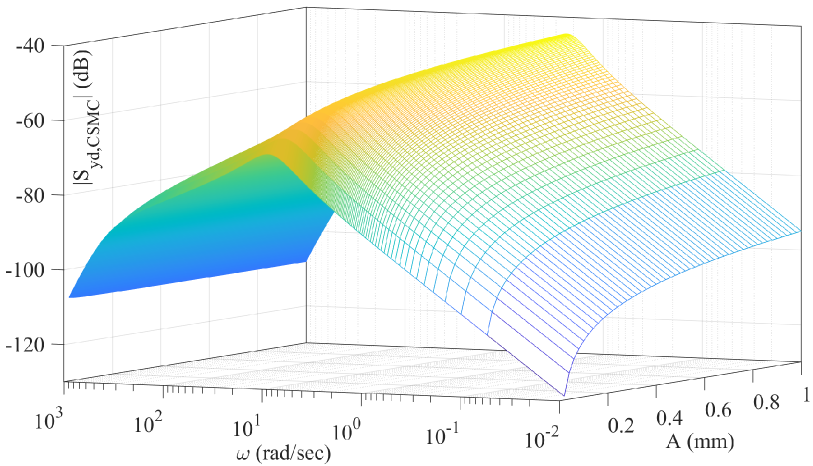
Figure 1: Frequency-amplitude-dependent magnitude characteristics of the disturbance sensitivity function (5) of the CSMC control loop

Note that the otherwise unknown upper bound $L$ was tuned based on the numerical simulations and experiments so that the residual oscillations of the output $y(t)$ at steady-state remain acceptably low, cf. further with section V. From Fig. 1, one can recognize that the amplitude dependency of the disturbance affecting the output is remarkable for both, lower frequency range and peak of the $S_{yd,CSMC}$ sensitivity function. At the same time, the disturbance sensitivity becomes less $A$-dependent for higher frequency range, thus making CSMC-control rather invariant to amplitude of the residual harmonic oscillations when the disturbance frequency grows. Here we note that the residual oscillations of the CSMC-controlled output can be estimated, according to [12], as

$$A=L\Bigl{(}\frac{2\alpha_{1}\lambda_{1}}{\pi\mathbb{K}^{2}(1-\mathbb{K}^{2})}\Bigr{)}^{3/2}\mu^{3}\quad\hbox{ and }\quad\omega=\frac{\mathbb{K}}{\mu}.$$ (6)

Here $A$ is the amplitude of steady-state harmonic of $y$ at the frequency $\omega$, after finite-time convergence of the CSMC. Therefore, the steady-state accuracy of CSMC control loop is bounded by (6) for each solution of HB equation. Recall that the amplitude of the residual output oscillations is predictable, provided the upper bound of the perturbation’s Lipschitz constant and actuator’s time-constant are known.

III Control Problem and System Description

We consider the problem of a standard output feedback control loop, see Fig. 2, with the measurable dynamic state $y(t)$ of interest and matched disturbance value $d(t)$. Note that all signals in the block diagram of Fig. 2 are purposefully denoted in Laplace domain, where $s$ is the complex Laplace variable, this for the sake of compatibility with the transfer functions in use. Since our prime focus is on the disturbance rejection, we assume zero reference i.e. $w(t)=0$ so that the control error yields $e=-y$. The system plant can be sufficiently approximated by the second-order transfer function $G(s)$, from the input force $u$ to the output relative displacement $y$. Note that the input-output characteristics of a motion system can be additionally subject to a fast parasitic dynamics of the actuator $D(s)$. Worth noting is that the latter belongs to the main application-related problems of the sliding mode controllers, causing the steady-state oscillations, known also as chattering.

Figure 2: Standard output feedback control loop.

The applied feedback controller is $C$, while for linear feedback controls, like the PID one which is benchmarking in this work, the corresponding transfer function $C(s)$ is in place. For the nonlinear PID-like sliding mode control (CSMC), $C$ constitutes a continuous mapping $e\in\mathbb{R}\mapsto u\in\mathbb{R}$.

The main focus of our investigations is on the comparative analysis of the control error suppression, i.e. by means of a controller $C$, when the dynamic disturbance $d(s)$ of certain frequency-band affects the closed-loop system as in Fig. 2. Note that due to a finite-time convergence of CSMC and, hence, its transient behavior that depends directly on the admissible control gains and the initial conditions, only steady-state behavior can be adequately compared between CSCM and PID. Furthermore, it is worth recalling that the CSMC is efficient to deal with systems affected by non-vanishing Lipschitz perturbations [12]. Therefore, the disturbance of a particular frequency, like a one defined later in (11), will have upper bound of the Lipschitz constant $L=A_{d}\omega_{d}$. Accordingly, for the known upper bound $\max A_{d}$ of the disturbance value, the admissible bandwidth of the closed-loop with CSMC is $\max\omega_{d}\leq L(\max A_{d})^{-1}$. In case of a linear feedback control $C(s)$, the same admissible bandwidth $\max\omega_{d}$ can be assumed, for the sake of comparison, while the superposition principle yields the linear closed-loop control system invariant to the amplitude $A_{d}$ of disturbances. Note that this requires, however, an unsaturated control value for the system plant $G(s)$.

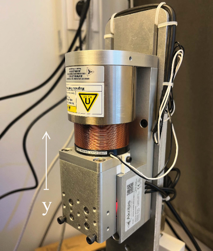
Figure 3: Experimental setup of the motion system

The second-order system under investigation in this study is an electro-mechanical drive depicted in Fig. 3. The induced relative displacement $y(t)$ is indirectly measured by the contactless inductive displacement sensor with a nominal repeatability of $\pm 12$ micrometers. While all mechanical elements are rigid, and the system dynamics is inherently of the second-order, with one free integrator, the nominal electrical time constant of the actuator is $\mu=1.2$ msec. Note that this knowledge of a parasitic actuator dynamics will be explicitly used when analyzing fast oscillations of the continuous sliding mode control, cf. section II. Furthermore, it is known that the system discloses a relatively high level of the sensor and process noise. The former is due to a contactless sensing, while the latter is due to additional parasitic by-effects which are not captured by the simplified linear modeling, cf. sections II-A and III-A. The real-time control board operates the system with the set sampling rate of 5 kHz. More details on the experimental system can be found in [18], with principal difference that in the present work an oscillating payload is purposefully detached from the drive. The available and the identified system parameters are given below.

III-A Modeled and Identified System Plant

The principal dynamics of the plant under consideration are assumed to be represented by

$$m\ddot{y}(t)+\sigma\dot{y}(t)=\frac{\Psi}{R}\tilde{u}(t)-mg,$$ (7)

with input $\tilde{u}(t)$ (in volts) and measurement $y(t)$ (in meters). The values of the moving mass $m$, back electromotive force constant $\Psi$, and resistance $R$ are given by

$$m=0.538\>\mathrm{kg},\quad\Psi=17.16\,\mathrm{\frac{Vs}{m}},\quad R=5.32\,\mathrm{\frac{V}{A}}$$ (8)

and originate from the weight measurement and the actuator data sheet [19]. Note that the gravitational force $F_{\mathrm{g}}=-mg$ with the gravity constant $g=9.81\,\mathrm{ms^{-2}}$ can be directly compensated with $u_{\mathrm{g}}=mgR\Psi^{-1}$ and is, therefore, not a part of further discussions. In order to estimate the unknown damping parameter $\sigma>0$, we apply $\tilde{u}=u+u_{\mathrm{g}}$ leading to

$$\frac{m}{\sigma}\ddot{y}(t)+\dot{y}(t)=\frac{\Psi}{R\sigma}u(t).$$ (9)

Using the Laplace transform, with zero initial conditions, the plant’s transfer function reads

$$G(s)=\frac{K}{s(\tau s+1)}~{}\mathrm{with}~{}K=\frac{\Psi}{R\sigma},~{}\tau=\frac{m}{\sigma}.$$ (10)

Due to the free integrative behavior and bounded position measurement $y\in[0\,\mathrm{mm},18\,\mathrm{mm}]$, the identification experiments are conducted in a closed-loop, as in Fig. 2. In order to minimize the noise amplification and without exciting further dynamics, a pure proportional controller with a relatively low gain $C=100$ is utilized here for the parameter identification experiments. Starting from the middle of the actuator range at steady-state $y_{0}=9\,\mathrm{mm}$, a sinusoidal input disturbance

$$d(t)=A_{\mathrm{d}}\sin(\omega_{\mathrm{d}}t)$$ (11)

is applied for exciting the system.

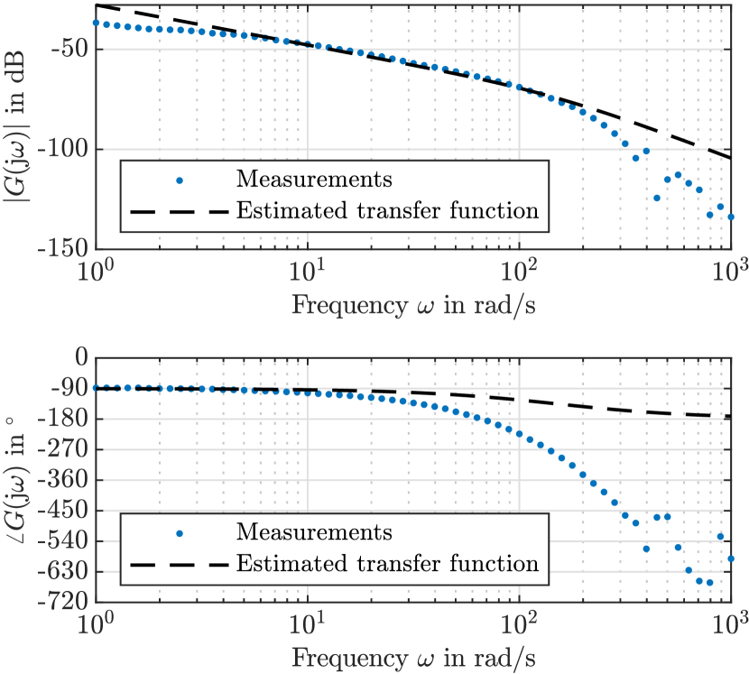
Figure 4: Bode plot of the experimental data and estimated transfer function.

The amplitude $A_{\mathrm{d}}\in[0.7\,\mathrm{V},1.5\,\mathrm{V}]$ is chosen to ensure sufficient excitation without input- and state-saturation, in accord with the frequency range $\omega_{\mathrm{d}}\in[1\,\mathrm{rad/s},\,1000\,\mathrm{rad/s}]$. A measurement of 20 periods at steady-state is utilized for the frequency response estimation at each frequency. With use of the auto-correlation $R_{\mathrm{uu}}(\cdot)$ and cross-correlation functions $R_{\mathrm{uy}}(\cdot)$, the magnitude and phase at $\omega_{\mathrm{d}}$ can be calculated as, cf. with e.g. [20],

$$\left|G(\mathrm{j}\omega_{\mathrm{d}})\right|=\frac{R_{\mathrm{uy,max}}}{R_{\mathrm{uu}}(0)}\quad\text{and}\quad\angle G(\mathrm{j}\omega_{\mathrm{d}})=-\omega_{\mathrm{d}}\Delta\tau,$$ (12)

where $\Delta\tau$ is the time lag between the two correlation functions. The resulting Bode plot of the experimentally collected frequency-response data is depicted in Fig. 4.

The phase for low frequencies corresponds to the integrating behavior. However, high frequencies show an increasing time delay in terms of a phase lag which is not covered by the second-order model (10). Only the magnitude plot is therefore used for the transfer function estimation. The least-squares optimal fit for $G$, using $\left|G(\mathrm{j}\omega_{\mathrm{d}})\right|$ with $\omega_{\mathrm{d}}\in[4\,\mathrm{\frac{rad}{s}},380\,\mathrm{\frac{rad}{s}}]$, results in $\sigma=80.4884$. This yields the

$$K=0.0408\quad\text{and}\quad\tau=6.684\,\mathrm{ms}$$ (13)

parameter values. The Bode plot of the estimated $G(j\omega)$ is equally depicted in Fig. 4 over the measurements.

IV Robust Linear PID Control

In this section, a derivation of the two-step procedure for a robust PID controller design, resting on an underlying PD control with stable pole-zero cancelation and upper bound of the disturbance sensitivity function, is provided.

IV-A Controller Design

In order to reduce the design complexity of the linear PID controller and, correspondingly, limit the tuning degrees-of-freedom to only the overall control gain and integration time constant, a stable pole-zero cancelation is first performed. To this end, applying the underlying PD controller

$$C_{\mathrm{PD}}(s)=\gamma(\tau s+1)$$ (14)

with the proportional gain $\gamma$ and derivative time constant $\tau$, the pole of the plant $G(s)$ at $p=-\frac{1}{\tau}$ is canceled. Therefore, only the $\gamma$-gain can be used for further control tuning. Since disturbance rejection is of our major interest, the input disturbance sensitivity function

$$S_{\mathrm{yd}}(s)=\frac{G(s)}{1+G(s)C(s)}$$ (15)

is considered. Utilizing the PD controller (14) results in

$$S_{\mathrm{yd,PD}}(\mathrm{j}\omega)=\frac{-K}{(\omega\tau-\mathrm{j})(\omega-\mathrm{j}K\gamma)},$$ (16)

with the corresponding magnitude response

$$\left|S_{\mathrm{yd,PD}}(\mathrm{j}\omega)\right|=\frac{K}{\sqrt{\omega^{2}\tau^{2}+1}\sqrt{\omega^{2}+K^{2}\gamma^{2}}}.$$ (17)

Note that this approaches its maximum at steady-state, i.e.

$$\left|S_{\mathrm{yd,PD}}(\mathrm{j}\omega)\right|\Big{|}_{\omega=0}=\frac{1}{\gamma}>\left|S_{\mathrm{yd,PD}}(\mathrm{j}\omega)\right|\quad\forall\omega>0,$$ (18)

which is equivalent to

$$\left\|S_{\mathrm{yd,PD}}\right\|_{\infty}=\frac{1}{\gamma}.$$ (19)

Therefore, for a given worst case amplification of the matched disturbance, the proportional gain $\gamma$ is chosen as its inverse.

However, in order to ensure the steady-state accuracy, we make use of an (improper) PID controller

$$C_{\mathrm{PID}}(s)=\frac{\gamma(\tau s+1)(T_{\mathrm{I}}s+1)}{T_{\mathrm{I}}s}$$ (20)

with the integration time constant $T_{\mathrm{I}}$ as a further tuning parameter. This leads to the corresponding sensitivity function $S_{\mathrm{yd,PID}}$ with the magnitude characteristics

$$\left|S_{\mathrm{yd,PID}}(\mathrm{j}\omega)\right|=\frac{KT_{\mathrm{I}}\omega}{\sqrt{(K\gamma-T_{\mathrm{I}}\omega)^{2}+(KT_{\mathrm{I}}\gamma\omega)^{2}}\sqrt{\tau^{2}\omega^{2}+1}}.$$ (21)

In order to utilize the previous considerations, we show that (21) is bounded by $\left\|S_{\mathrm{yd,PD}}\right\|_{\infty}$, i.e.

$$\left|S_{\mathrm{yd,PID}}(\mathrm{j}\omega)\right|\leq\frac{1}{\gamma}\quad\forall\omega>0$$ (22)

holds true. This can be seen by considering

$$\left|S_{\mathrm{yd,PID}}(\mathrm{j}\omega)\right|^{2} =\frac{(KT_{\mathrm{I}}\omega)^{2}}{\left[(K\gamma-T_{\mathrm{I}}\omega)^{2}+(KT_{\mathrm{I}}\gamma\omega)^{2}\right]\underbrace{(\tau^{2}\omega^{2}+1)}_{>1\,\forall\omega,\tau>0}}$$

$$\leq\frac{(KT_{\mathrm{I}}\omega)^{2}}{(K\gamma-T_{\mathrm{I}}\omega)^{2}+(KT_{\mathrm{I}}\gamma\omega)^{2}}\equiv\Xi(\mathrm{j}\omega)$$

and knowing that $K,T_{\mathrm{I}},\omega>0$, which yields

$$\Xi(\mathrm{j}\omega)=\frac{1}{\left(\frac{K\gamma-T_{\mathrm{I}}\omega}{KT_{\mathrm{I}}\omega}\right)^{2}+\gamma^{2}}\leq\frac{1}{\gamma^{2}}.$$

Thus, the relation (22) becomes evident and can be used to determine an appropriate proportional gain for a given minimal input disturbance attenuation. The conservativeness of such design is discussed in section IV-B, for the specific case of the given plant and value for $\gamma$.

The free tuning parameter $T_{\mathrm{I}}$ is chosen based on the frequency characteristics of the open-loop and a predefined phase margin $\Phi$. The open-loop transfer function for zero initial conditions is given by

$$L(s)=C_{\mathrm{PID}}(s)\,G(s)=\frac{K\gamma(T_{\mathrm{I}}s+1)}{T_{\mathrm{I}}s^{2}}$$ (23)

and consists of a double-integrator and one stable zero. Therefore, the corresponding phase never crosses $-180^{\circ}$, leading to a (theoretically) infinite gain margin. However, the phase margin $\Phi$ can be used as a further robustness measure, especially with respect to additional phase lags. For this purpose, consider the amplitude and phase at open-loop crossover frequency $\omega_{\mathrm{s}}$, given by

$$\left|L(\mathrm{j}\omega_{\mathrm{s}})\right| =1$$ (24a)

$$\pi+\arg(L(\mathrm{j}\omega_{\mathrm{s}})) =\Phi.$$ (24b)

From (23) it can be seen that

$$L(\mathrm{j}\omega)=\frac{-K\gamma(1+\mathrm{j}T_{\mathrm{I}}\omega)}{T_{\mathrm{I}}\omega^{2}}=-\frac{K\gamma}{T_{\mathrm{I}}\omega^{2}}-\mathrm{j}\frac{K\gamma}{\omega}$$

and, hence, at $\omega_{\mathrm{s}}$ one obtains

$$|L(\mathrm{j}\omega_{\mathrm{s}})| =\frac{K\gamma\sqrt{1+\omega_{\mathrm{s}}^{2}T_{\mathrm{I}}^{2}}}{\omega_{\mathrm{s}}^{2}T_{\mathrm{I}}}\quad\text{and}$$ (25a)

$$\arg\left(L(\mathrm{j}\omega_{\mathrm{s}})\right) =\arctan\left(T_{\mathrm{I}}\omega_{\mathrm{s}}\right)-\pi,\quad T_{\mathrm{I}},\omega_{\mathrm{s}}>0.$$ (25b)

The combination of (24) and (25) yields

$$\omega_{\mathrm{s}} =\frac{K\gamma\sqrt{1+\tan^{2}(\Phi)}}{\tan(\Phi)}\quad\text{and}$$ (26a)

$$T_{\mathrm{I}} =\frac{\tan(\Phi)}{\omega_{\mathrm{s}}}.$$ (26b)

The above developments result in the two-step procedure for a dedicated PID controller design:

1. Set worst case disturbance amplification $S_{\mathrm{max}}$ leading to

   $$\gamma=\frac{1}{S_{\mathrm{max}}}.$$ (27)

2. Set the desired phase margin $\Phi$ and calculate

   $$T_{\mathrm{I}}=\frac{\tan^{2}(\Phi)}{K\gamma\sqrt{1+\tan^{2}(\Phi)}}.$$ (28)

With the parameters $\tau$, $\gamma$ and $T_{\mathrm{I}}$, the PID controller (20) is entirely determined.

IV-B Application of PID Controller

The design approach developed above is now utilized to determine the PID controller for the identified plant model $G$. For a good disturbance rejection and robustness, we choose

$$S_{\mathrm{max}}=-52\,\mathrm{dB}\quad\text{and}\quad\Phi=60^{\circ}$$

leading to

$$\gamma=400\quad\text{and}\quad T_{\mathrm{I}}=0.092\,\mathrm{s}.$$ (29)

The magnitude plot of $S_{\mathrm{yd}}$, using the underlying PD controller, is depicted in Fig. 5 opposite to the PID controller for a large variation of the integration time constant $T_{\mathrm{I}}$. Obviously, the maximum disturbance amplification is only little dependent on the value of $T_{\mathrm{I}}$, while a clear asymptotic reduction for lower frequencies is evident. The PID controller with $T_{\mathrm{I}}=0.1$ s, cf. with the determined parameters (29), provides certain optimality in shaping the disturbance sensitivity function. That means without sharp peak of $|S_{\mathrm{yd}}|$ and without a flat plateau of $|S_{\mathrm{yd}}|\rightarrow S_{\max}$ upper bound dictated by the underlying PD control.

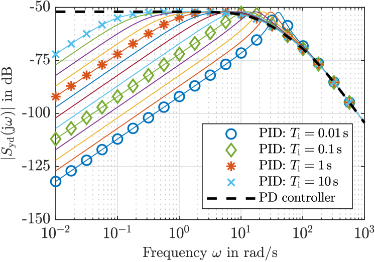
Figure 5: Magnitude plot of the input disturbance sensitivity function using a PD controller opposite to PID controllers with the different integration time constants $T_{\mathrm{I}}\in[0.01\,\mathrm{rad/s},~{}10\,\mathrm{rad/s}]$.

A closer look at the $\mathcal{H}_{\infty}$ norms for a variation of $T_{\mathrm{I}}$ in the relevant range, see Fig. 6, illustrates (19) and (22). Worth noting here is that for this set of parameters, the above mentioned conservativeness of (22) is limited to $0.31\,\mathrm{dB}$.

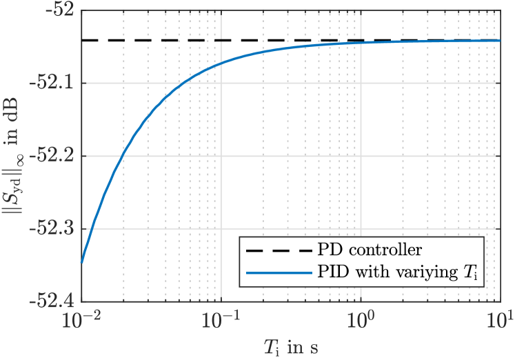
Figure 6: $\mathcal{H}_{\infty}$ norms of the disturbance sensitivity functions from Fig. 5.

For the ease of implementation and better comparison with the PID-like sliding mode control, the parallel form of the PID controller $C_{\mathrm{PID}}$ (20) reads as

$$\bar{C}_{\mathrm{PID}}(s)=K_{\mathrm{p}}+K_{\mathrm{I}}\frac{1}{s}+K_{\mathrm{D}}s,$$ (30)

with the proportional, integral and derivative gains as

$$K_{\mathrm{p}} =\gamma\frac{T_{\mathrm{I}}+\tau}{T_{\mathrm{I}}}=429.064,$$ (31)

$$K_{\mathrm{I}} =\frac{\gamma}{T_{\mathrm{I}}}=4348.267,$$ (32)

$$K_{\mathrm{D}} =\gamma\tau=2.674.$$ (33)

Here worth mentioning is that the parameters result directly from a comparison of coefficients between $C_{\mathrm{PID}}$ and $\bar{C}_{\mathrm{PID}}$.

V Experimental Study

In this section, we provide an experimental comparison of the PID controller, designed according to section IV, and the PID-like CSMC controller, cf. section II. At first, we recall and tune a robust exact differentiator, which is required for both controllers in order to use $\dot{y}(t)$ in feedback. Then, we show an experimental evaluation of the PID controller that confirms analysis and performance of the two-step procedure developed in section IV. Finally, we compare both the PID and CSMC controllers in suppressing a broadband disturbance.

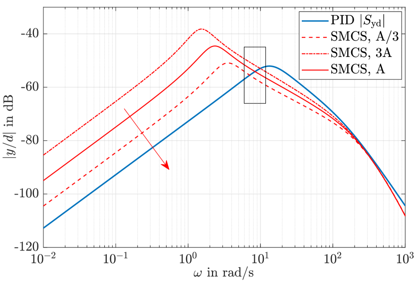
Figure 7: Magnitude plot of the $d$ to $y$ transfer characteristics: the disturbance sensitivity function $S_{yd}$ with PID control versus the amplitude-dependent harmonic balance approximation with CSMC control, for three exemplary amplitudes $3A$, $A$, $A/3$ of steady-state $y$ (differing by order of magnitude).

For the designed CSMC and PID controllers, the $d(j\omega)$ to $y(j\omega)$ transfer characteristics, with the describing function-based approximation (5) and disturbance sensitivity function $S_{yd}(j\omega)$, respectively, are shown in Fig. 7. For the PID control loop, it shows a maximum of $\hat{S}_{\mathrm{max}}=-52.08\,\mathrm{dB}$ at $\omega_{\mathrm{max}}=13.31\,\mathrm{rad/s}$. Therefore, the largest impact on the output value is expected from the disturbances with a frequency around $\omega_{\mathrm{max}}$. The magnitude plot of the amplitude-dependent harmonic balance approximation for CSMC control, i.e. (5), is shown for steady-state of $y$ with the exemplary amplitudes $A=0.001$ m and its $3A$ and $A/3$ variations, cf. with Fig. 10. Shrinking of the disturbance sensitivity characteristics of CSMC control is clearly visible for amplitude reduction, marked by an arrow in Fig. 7. One can recognize that starting from certain frequencies (see rectangular mark in Fig. 7) the expected disturbance rejection becomes better comparing to PID. It is also evident that for a further decreasing amplitude of $y$-oscillations, the $|d/y|$ plot of CSMC will lie entirely below the $|S_{yd}(j\omega)|$ plot of the linear feedback control.

V-A Robust Exact Differentiator

In order to obtain an estimate of the output derivative $\dot{y}(t)$, to be practically suitable for the feedback loop, we apply a robust exact differentiator [21] (further as RED), which is based on the sliding-mode estimation principles, see e.g. [1]. Its remarkable features are an insensitivity to the bounded noise (provided the Lipschitz constant of n-th time-derivative is available) and a finite-time convergence. This makes a RED, at least theoretically, free of a phase lag. Recall that the latter is otherwise deteriorating the loop performance if a low-pass filtering of the differentiated measurement of $y(t)$ is used. The second-order RED, cf. [22], with the parametrization according to [23] is given by

$$\dot{x}_{0} =x_{1}+3.1~{}r~{}|y-x_{0}|^{\frac{2}{3}}~{}\mathrm{sign}(y-x_{0}),$$ (34a)

$$\dot{x}_{1} =x_{2}+3.2~{}r^{2}~{}|y-x_{0}|^{\frac{1}{3}}~{}\mathrm{sign}(y-x_{0}),$$ (34b)

$$\dot{x}_{2} =1.1~{}r^{3}~{}\mathrm{sign}(y-x_{0}),$$ (34c)

where the scaling factor $r>0$ is the single design parameter. It is worth noting that $r^{n+1}$ (in our case $r^{3}$) corresponds to the Lipschitz constant $L$ of the highest derivative ${y}^{(n)}$, cf. [23].

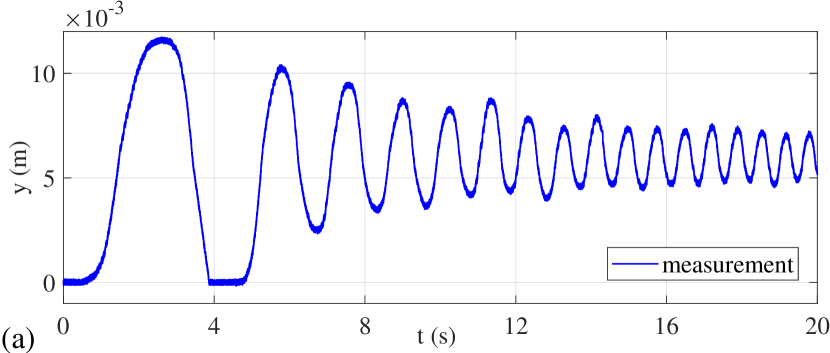
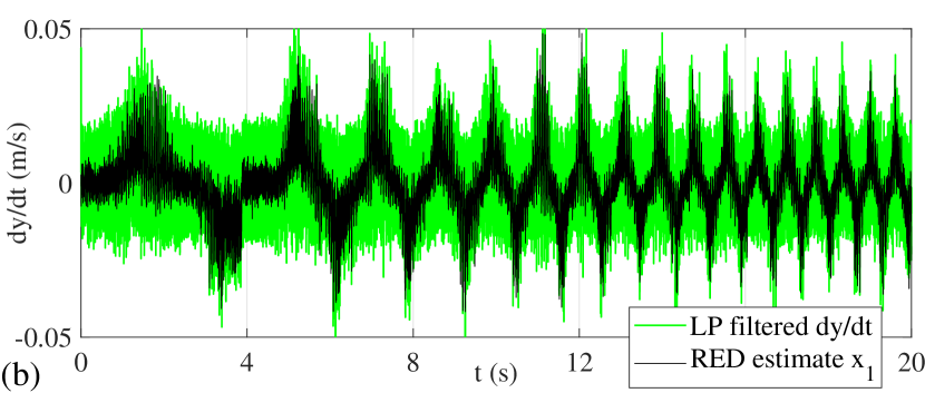
Figure 8: Exemplary evaluation of the 2nd order RED with $r=8$: the measured output value in (a) and RED estimate $x_{1}$ over the low-pass (LP) filtered discrete time derivative of $y$ in (b).

Note that the second-order (and not first-order) RED is purposefully used here, in order to obtain a smoother estimate $x_{1}(t)$ of the output derivative. Recall that the second-order RED provides $x_{0}(t)=y(t)$, $x_{1}(t)=\dot{y}(t)$, $x_{2}(t)=\ddot{y}(t)$, for all $t>t_{c}$, where $t_{c}$ is a finite convergence time. The scaling factor $r=8$ was experimentally tuned on the collected $y(t)$ data, for which an up-chirp signal until $\omega=80$ rad/s disclosed a still satisfying match between the $x_{1}(t)$ estimate and theoretically calculated $\dot{y}(t)$. An exemplary evaluation of the RED (34) with $r=8$ is shown in Fig. 8, in comparison with the discrete time derivative of the measured signal $y$, which is then low-pass filtered with the cutoff frequency of 100 Hz.

V-B Evaluation of PID Controller

In order to evaluate efficiency of the proposed PID design procedure, as well as the accuracy of the model fit and the associated linear loop shaping, cf. section IV, the sinusoidal input disturbance $d(t)$ (given by eq. (11)) is used in experiments. The assigned amplitude is $A_{\mathrm{d}}=1\,\mathrm{V}$ and the frequencies selected around $\omega_{\mathrm{max}}$ are

$$\omega_{\mathrm{d,1}}=5\,\mathrm{\frac{rad}{s}},\quad\omega_{\mathrm{d,2}}=10\,\mathrm{\frac{rad}{s}}\quad\text{and}\quad\omega_{\mathrm{d,3}}=20\,\mathrm{\frac{rad}{s}}.$$

The experimental results are depicted in Fig. 9 by disclosing the control errors. Evaluating the theoretically expected disturbance attenuation at $\omega_{\mathrm{d,1,\ldots,3}}$ i.e. $|\tilde{S}_{\mathrm{yd}}(\mathrm{j}\omega_{\mathrm{d,1,\ldots,3}})|=\{-58.6,\,-52.9,\,-53.8\}\,\mathrm{dB}$ and comparing these values with the corresponding numbers calculated out from the experiments $\{-57.5,\,-52.6,\,-50.1\}\,\mathrm{dB}$, cf. Figs. 7 and 9, one can recognize a good accordance between both.

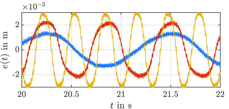
Figure 9: Measured control error $e$ of $\bar{C}_{\mathrm{PID}}$ for the disturbance attenuation.

V-C Controllers Comparison for Broadband Disturbances

The CSMC and PID controllers, both designed according to sections II and IV respectively, are evaluated experimentally and compared to each other in the disturbance rejection. The applied disturbance signal is an up-chirp

$$d(t)=A_{d}\sin\bigl{(}(\omega_{0}+\alpha t)\,t\bigr{)}$$

with a linearly increasing frequency, i.e. $\alpha>0$, and the start and end frequencies of 0.06 rad/sec and 30 rad/sec, correspondingly. The chirp runtime of 60 sec ensures that the transient, correspondingly convergence, phase of the control response (which one is relatively long for the realizable gain values of CSMC) is passed at lower frequencies, see Fig. 10 (a). Following to that, a steady-state disturbance rejection behavior can be compared for the times about $t>10$ sec.

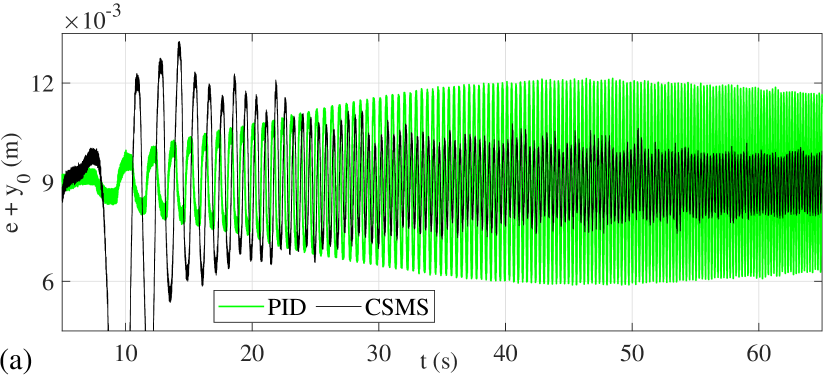
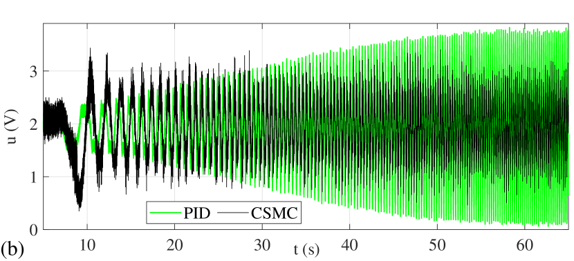
Figure 10: Experimental results of the PID and CSMC controllers on rejection of the up-chirp disturbance with bandwidth 0.06–30 rad/s: the control error (around the reference position $y_{0}=9$ mm) in (a) and control signal in (b)

It can be seen that the error pattern of the PID control follows the expected shape of the disturbance sensitivity function, cf. Fig. 7. On the contrary, the CSMC control error is continuously decreasing with an increasing frequency, that corresponds to the CSMC sensitivity function charts that depend of the amplitude of the main harmonic of chattering at steady-state, cf. section II. The period where the control error of both PID and CSCM are approximately the same, i.e. at the time about 24 sec, corresponds to the disturbance frequency $w_{d}\approx 9.5$ rad/sec, cf. Fig. 7. Regarding the control values, see Fig. 10 (b), one can recognize that for the PID control, the signal pattern is also inline with the frequency response of the closed-loop system (cf. Fig. 2). For that, the transfer characteristics between $d(j\omega)$ and $u(j\omega)$ are indicative. One can recognize that with an increasing angular frequency, the amplitude of the PID control value $u(t)$ is also growing, thus resulting in a higher power and, correspondingly, energy consumption. On the contrary, the control value of CSMC keeps an almost constant amplitude level, that speaks for a lower power consumption. Also recall that for finite-time convergence of CSMC the control signal tends to the opposite value of perturbation, that is the case with a chirp disturbance of a constant amplitude, Fig. 10 (b).

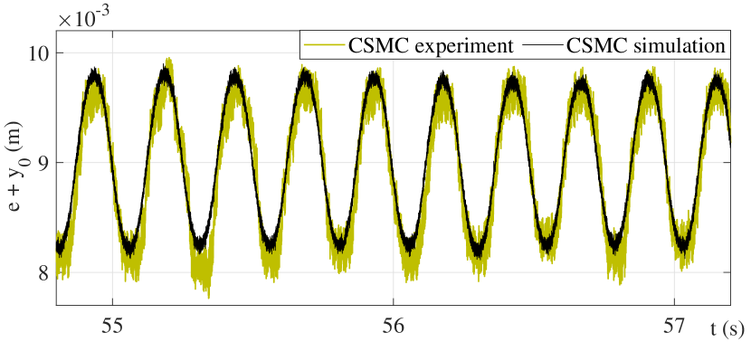
Figure 11: Comparison between the simulated and experimental response of CSMC control; experimental data are from higher-frequencies from Fig. 10.

The comparison between the simulated and experimental response of the closed loop with CSMC controller is exemplary shown in Fig. 11. Here the same data of a higher-frequency clipping from Fig. 10 is used. Note that in the numerical simulation of the system (7), augmented by $d$ with the control (2), an additional band-limited white noise is added to the output $y(t)$, so as to bring the modeled control system behavior closer to the real experiments. Up to the noise level, the simulated and experimental response of the CSMC-controlled output coincide well with each other, cf. Fig. 11.

VI Conclusions

A PID-like continuous sliding mode (CSMC) controller, known to be robust for rejection of the matched Lipschitz continuous perturbations, was analyzed in terms of a disturbance sensitivity function. This frequency-domain approach, which takes additionally into account the amplitude of steady-state harmonics of the CSMC control loop (when perturbed by the actuator) allows a comparison with standard linear feedback controllers. Due to the structural similarity, i.e. with feedback of the output, its derivative, and integral, the CSMC was compared with a standard linear PID control, designed also for rejection of the matched disturbances. Both controllers were compared experimentally as the fair competitors. The developed two-step procedure for a robust PID controller design yields two tunable parameters, the overall control gain and the integration time constant. Both are shown as associated with the H-infinity norm of the disturbance sensitivity function and with the desired phase margin, respectively. The CSMC control parametrization follows exactly the analysis and developments provided in [12], yielding only one tunable parameter, which is the scaling factor out from the Lipschitz constant of perturbations. The comparative study of both controllers is made for the second-order experimental motion system with additional fast parasitic dynamics of the actuator. The two-parameters linear model of the system plant is identified in frequency domain and shown to be sufficient for design of the feedback controllers. For the time derivative of the output, required for both PID and CSMC controls, the robust second-order sliding-mode differentiator is designed and used in experiments. The PID and CSMC controllers are evaluated experimentally on rejection of a broadband input disturbance, which is an up-chirp between 0.06 rad/sec and 30 rad/sec. The resulted control performance is shown to be fully inline with the theoretically expected (i) disturbance sensitivity characteristics (i.e. sensitivity function) of the PID control loop, and (ii) describing-function based prediction of the steady-state harmonic oscillations (i.e. chattering) of the CSMC control loop. The CSMC disturbance rejection performance is shown to be clearly less frequency-sensitive in the control error pattern, and more energy efficient as for the control signal amplitude. At the same time, the transient behavior of CSMC control disclosed inferior, comparing to the PID one, that for the maximal achievable $L$-scaling factor of the CSMC parametrization. It can be noted that describing the propagation of slow signals through the oscillating system, correspondingly transient behavior, might require the concept of an equivalent gain, cf. [24]. This is, however, out of scope of the present work. The $L$-scaling factor, also related to the actuator dynamics, proved experimentally to be most sensitive for application of the CSMC control. In summary, the demonstrated practical comparison of PID and CSMC controllers allows for a better understanding and distinction of the application benefits and challenges of their use in compensating for amplitude- and band-specific disturbances.

References

- [1] Y. Shtessel, C. Edwards, L. Fridman, and A. Levant, Sliding mode control and observation. Springer, 2014.
- [2] I. Boiko, “Frequency-domain analysis of fast and slow motions in sliding modes,” Asian Journal of Control, vol. 5, no. 4, pp. 445–453, 2003.
- [3] I. Boiko, “Oscillations and transfer properties of relay servo systems - the locus of a perturbed relay system approach,” Automatica, vol. 41, no. 4, p. 677–683, 2005.
- [4] A. Levant, “Sliding order and sliding accuracy in sliding mode control,” International journal of control, vol. 58, no. 6, pp. 1247–1263, 1993.
- [5] C. A. Zamora, J. A. Moreno, and S. Kamal, “Control integral discontinuo para sistemas mecánicos,” in 2013 Congreso Nacional de Control Automático (CNCA AMCA), 2013, pp. 11–16.
- [6] J. A. Moreno, “Discontinuous integral control for mechanical systems,” in IEEE 14th International Workshop on Variable Structure Systems (VSS), 2016, pp. 142–147.
- [7] S. Kamal, J. A. Moreno, A. Chalanga, and B. Bandyopadhyay, “Continuous terminal sliding-mode controller,” Automatica, vol. 69, pp. 308–314, 2016.
- [8] S. Laghrouche, M. Harmouche, and Y. Chitour, “Higher order super-twisting for perturbed chains of integrators,” IEEE Transactions on Automatic Control, vol. 62, no. 7, pp. 3588–3593, 2017.
- [9] E. Cruz-Zavala and J. A. Moreno, “Higher order sliding mode control using discontinuous integral action,” IEEE Transactions on Automatic Control, vol. 65, no. 10, pp. 4316–4323, 2019.
- [10] A. Mercado-Uribe and J. A. Moreno, “Discontinuous integral action for arbitrary relative degree in sliding-mode control,” Automatica, vol. 118, p. 109018, 2020.
- [11] J. A. Moreno, E. Cruz-Zavala, and Á. Mercado-Uribe, “Discontinuous integral control for systems with arbitrary relative degree,” in Variable-Structure Systems and Sliding-Mode Control, 2020, pp. 29–69.
- [12] U. Pérez-Ventura, J. Mendoza-Avila, and L. Fridman, “Design of a proportional integral derivative-like continuous sliding mode controller,” International Journal of Robust and Nonlinear Control, vol. 31, no. 9, pp. 3439–3454, 2021.
- [13] A. Levant, “Chattering analysis,” IEEE Transactions on Automatic Control, vol. 55, no. 6, pp. 1380–1389, 2010.
- [14] U. Pérez-Ventura and L. Fridman, “Design of super-twisting control gains: A describing function based methodology,” Automatica, vol. 99, pp. 175–180, 2019.
- [15] U. Pérez-Ventura and L. Fridman, “When is it reasonable to implement the discontinuous sliding-mode controllers instead of the continuous ones? frequency domain criteria,” International Journal of Robust and Nonlinear Control, vol. 29, no. 3, pp. 810–828, 2019.
- [16] A. Filippov, Differential Equations with Discontinuous Right-hand Sides. Dordrecht: Kluwer Academic Publishers, 1988.
- [17] A. Pisano and E. Usai, “Contact force regulation in wire-actuated pantographs via variable structure control and frequency-domain techniques,” Int. J. of Control, vol. 81, no. 11, pp. 1747–1762, 2008.
- [18] M. Ruderman, “One-parameter robust global frequency estimator for slowly varying amplitude and noisy oscillations,” Mechanical Systems and Signal Processing, vol. 170, p. 108756, 2022.
- [19] Akribis, “Voice coil motor user manual,” Apr. 2018.
- [20] R. Isermann and M. Münchhof, Identification of dynamic systems: an introduction with applications. Springer, 2011.
- [21] A. Levant, “Robust exact differentiation via sliding mode technique,” Automatica, vol. 34, no. 3, pp. 379–384, 1998.
- [22] J. A. Moreno, “Lyapunov function for Levant’s second order differentiator,” in IEEE 51st conference on decision and control, 2012.
- [23] M. Reichhartinger, S. Spurgeon, M. Forstinger, and M. Wipfler, “A robust exact differentiator toolbox for Matlab®/Simulink®,” IFAC-PapersOnLine, vol. 50, no. 1, pp. 1711–1716, 2017.
- [24] I. Boiko, M. Castellanos, and L. Fridman, “Describing function analysis of second-order sliding mode observers,” International journal of systems science, vol. 38, no. 10, pp. 817–824, 2007.