Galactic rotation dynamics in a new $f(\mathcal{R})$ gravity model

Abstract

We propose to test the viability of the recently introduced $f(\mathcal{R})$ gravity model in the galactic scales. For this purpose we consider test particles moving in stable circular orbits around the galactic center. We study the Palatini approach of $f(\mathcal{R})$ gravity via Weyl transformation, which is the frame transformation from the Jordan frame to the Einstein frame. We derive the expression of rotational velocities of test particles in the new $f(\mathcal{R})$ gravity model. For the observational data of samples of high surface brightness and low surface brightness galaxies, we show that the predicted rotation curves are well fitted with observations, thus implying that this model can explain flat rotation curves of galaxies. We also study an ultra diffuse galaxy, AGC $242019$ which has been claimed in literature to be a dark matter dominated galaxy similar to low surface brightness galaxies with a slowly rising rotation curve. The rotation curve of this galaxy also fits well with the model prediction in our study. Furthermore, we studied the Tully-Fisher relation for the entire sample of galaxies and found that the model prediction shows the consistency with the data.

I Introduction

A longstanding challenge in astrophysics and cosmology is the mystery of dark matter (DM) bertone ; swart ; tim ; frenk ; strigari . The missing mass problem was first predicted in the early 1930s by J. H. Oort oort while studying the motion of stars in the Milky Way. Around the same time similar evidences were reported by Swiss astronomer Fritz Zwicky, who studied the Coma Cluster zwicky ; Zwicky . Two prime evidences that insist on the existence of DM are the velocity rotation curve of galaxies rubin ; young ; borriello and the gravitational lensing young ; massey . American astronomer Vera Rubin, did pioneering work by conducting a study of rotation curves of 60 isolated galaxies garrett and established the idea of “missing mass”. Using the Planck data planck on the Cosmic Microwave Background (CMB) radiation, measurements of the cosmological parameters infer that the Universe is made up of $\sim 4-5\%$ baryons, $\sim 25\%$ non-baryonic dark matter, and $\sim 70\%$ dark energy. A few particles claimed as DM candidates Bertone ; feng are, namely, weakly interacting massive particles (WIMPs), standard model (SM) neutrinos, sterile neutrinos, axions, supersymmetric candidates (neutralinos, sneutrinos, gravitinos, axinos), etc. However, after almost eight decades since the development of the concept of DM, the DM particle is still missing from the table of elementary particles of nature, i.e. the fundamental nature of DM remains a mystery, and the problem of DM persists.

Over the past few decades various other issues, especially the flatness and horizon problems guth , and the riddle related to the late time cosmic acceleration reiss ; perlmutter have come to light, which specify that the standard cosmological model based on Einstein’s General Relativity (GR) and the particle physics standard model fails to explain the Universe at large scales. This has generated an increasing interest to explore alternative theories of gravity (ATGs) Clifton ; wagoner ; ronald ; yunes ; alsing , where gravitational interactions other than the ones described by GR were proposed. Within the broad area of ATGs, here we refer the modified theories of gravity (MTGs) capozziello ; clifton ; oikonomou ; odintsov ; sergei as the ATGs those were proposed to modify GR to provide solutions to emerging issues. The simplest class of MTGs is the $f(\mathcal{R})$ gravity faraoni ; felice . In these gravity theories the modification is made to the geometry part of Einstein’s field equations. This is done by replacing the Ricci scalar $\mathcal{R}$ of the Einstein-Hilbert action with a function $f(\mathcal{R})$ of $\mathcal{R}$. There are two main variational approaches to derive the field equations in $f(\mathcal{R})$ gravity, the metric formalism and the palatini formalism. In the metric formalism, matter is minimally coupled with the metric, and the energy-momentum tensor is independently conserved. In Palatini formalism, the metric as well as the connection are treated as independent variables. Here, the Riemann tensor as well as the Ricci tensor are constructed with the independent connection. Moreover, there are other formalisms which are found in the literature are the metric-affine formalism Sotiriou and the hybrid metric-Palatini formalism hybrid_metric_palatini . In the metric-affine formalism the matter action is considered as variable with respect to connection in contrast to the case of the Palatini formalism. The hybrid metric-Palatini formalism is the combination of the suitable elements of both metric and Palatini formalisms.

A plethora of research works have been dedicated to explain the effects of DM in MTGs riazi ; shtanov ; nashiba ; harko ; yuri ; katsuragawa ; lobo . As the concept of DM has mainly been indicated by irregularities in the galactic rotation curves, several MTGs have been proposed to study galactic rotation curves. Harko Harko investigated galactic rotation curves in MTGs with non-minimal coupling between matter and geometry. Capozziello et al. hybrid_metric_palatini studied rotation curves in hybrid metric-Palatini gravity model. Gergely et al. gergely considered the asymptotic behaviour of galactic rotation curves in brane world models. Several other studies capone ; sporea ; finch ; lin ; troisi ; salucci ; martins ; vipin have been carried out in different MTGs to explain galactic rotation curves. These studies have motivated us to study and explain the rotation curves in a viable $f(\mathcal{R})$ gravity model. Here we propose to investigate the rotation curves of galaxies in the Palatini $f(\mathcal{R})$ gravity taking into consideration the conformal transformation of the metric. It is basically a frame transformation from the Jordan frame to the Einstein frame goswami ; darabi ; yuri_shtanov ; olmo via a conformal factor. To this aim, we consider the new model dhruba ; Dhruba of $f(\mathcal{R})$ gravity, which has been recently introduced as a viable dark energy model of the theory. The main motive of the present study is to test the viability of this recent model in the galactic scales. We start by considering test particles around galaxies moving in stable circular orbits. The rotational velocity obtained by employing the new $f(\mathcal{R})$ gravity model has the Newtonian term as well as that coming from the modified geometry. The predicted rotational velocity from the model is fitted with observations of a few samples of high surface brightness (HSB), low surface brightness (LSB) and dwarf galaxies. Another addition to our work is the study of the ultra diffuse galaxies (UDGs). They are a fascinating class of galaxies with unusual properties, such as very high dokkum16 , or very low content of DM dokkum18 . Infact, UDGs are difficult to observe bothun91 ; bothun97 ; dokkum ; roman as well as to analyze ruiz ; forbes . We have investigated the behaviour of the rotation curve of a particular UDG, AGC $242019$ brook ; shi21 . The rotational velocity predicted the model fits well for this UDG. Furthermore, we also derive the Tully-Fisher relation tully ; brownstein ; mcgaugh for the new $f(\mathcal{R})$ gravity model.

Our work is organised as follows. In section II, we discuss the simplest type of modified gravity, i.e. the $f(\mathcal{R})$ gravity in the Palatini formalism. Here, we obtain the modified field equations in $f(\mathcal{R})$ gravity. The Weyl transformation from the Jordan frame to the Einstein frame and its implications on the Palatini $f(\mathcal{R})$ gravity is also discussed in this section. In section III, we study the dynamics of a test particle around the centres of galaxies in conformally transformed Palatini $f(\mathcal{R})$ gravity. In section IV, we derive the rotational velocity of the test particles in the recently proposed model of $f(\mathcal{R})$ gravity as mentioned above. In section V, we fit the predicted rotational velocity with observations as a test of the new $f(\mathcal{R})$ gravity model in galactic scales. Further, in section VI, we derive the Tully-Fisher relation for the model. Finally, in section VII we conclude and discuss the results of our work. Throughout our work we use the metric signature (- , +, +, +).

II Palatini $f(\mathcal{R})$ gravity and Weyl geometry

II.1 Field Equations

The action that defines $f(\mathcal{R})$ theories of gravity faraoni has the generic form:

$$S=\frac{1}{2\kappa^{2}}\int d^{4}x\sqrt{-g}\,f(\mathcal{R})+S_{m}\left[g^{\mu\nu},\Phi\right],$$ (1)

where $f(\mathcal{R})$ is a function of the Ricci scalar $\mathcal{R}=g^{\mu\nu}\mathcal{R}_{\mu\nu}$ and $\kappa^{2}=8\pi Gc^{-4}=1/M^{2}_{pl}$. $M_{pl}$ is the (reduced) Planck mass $\sim 2\times 10^{18}$ GeV. $S_{m}$ is the matter action that is independent of the connection but depends on the metric $g_{\mu\nu}$ and the matter field $\Phi$. Here, we will apply the Palatini formalism olmo ; jyatsna . As mentioned earlier, unlike the metric formalism, in the Palatini approach the torsion-free connection $\Gamma_{\mu\nu}^{\alpha}$ and the metric $g_{\mu\nu}$ are treated as the dynamical variables to be independently varied. Now, varying the action (1) with respect to the metric $g_{\mu\nu}$ we obtain the field equations as

$$f_{\mathcal{R}}(\mathcal{R})\,\mathcal{R}_{\mu\nu}-\frac{1}{2}f(\mathcal{R})\,g_{\mu\nu}=\kappa^{2}\,T_{\mu\nu},$$ (2)

where $f_{\mathcal{R}}(\mathcal{R})$ is the derivative of $f(\mathcal{R})$ with respect to $\mathcal{R}$ and the energy-momentum tensor $T_{\mu\nu}$ is given by

$$T_{\mu\nu}\left[g^{\mu\nu},\Phi\right]=\frac{-\,2}{\sqrt{-\,g}}\frac{\delta\left(\sqrt{-\,g}\,S_{m}\left[g^{\mu\nu},\Phi\right]\right)}{\delta\,g_{\mu\nu}}.$$ (3)

Again, the variation of the action (1) with respect to the connection $\Gamma_{\mu\nu}^{\alpha}$ gives,

$$\nabla_{\alpha}\!\left(\sqrt{-\,g}\,f_{\mathcal{R}}(\mathcal{R})\,g^{\mu\nu}\right)=0.$$ (4)

It should be noted that when $f(\mathcal{R})=\mathcal{R}$, equation (2) gives the Einstein’s field equations and equation (4) simply becomes the definition of the Levi-Civita connection in GR. This means that in the limit $f(\mathcal{R})=\mathcal{R}$, the Palatini approach leads to GR as expected. Trace of equation (2) is given as

$$\mathcal{R}f_{\mathcal{R}}(\mathcal{R})-2f(\mathcal{R})=\kappa^{2}\,T_{\mu}^{\mu}.$$ (5)

This expression shows that $\mathcal{R}=g^{\mu\nu}\mathcal{R}_{\mu\nu}(\Gamma)$ can be algebraically solved in terms of the trace of energy-momentum tensor $T\equiv T_{\mu}^{\mu}=g^{\mu\nu}T_{\mu\nu}$ which leads to $\mathcal{R}=\mathcal{R}(T)$ and $f_{\mathcal{R}}=f_{\mathcal{R}}(T)$ as functions of matter but not of the torsion-free connection.

II.2 Weyl transformation

Named after Hermann Weyl, the Weyl transformation darabi ; olmo is a frame transformation from the Jordan frame to the Einstein frame. Usually this transformation is essential to get the minimally coupled scalar degree of freedom in the Einstein frame from the conventionally non-minimally coupled one in the Jordan frame in $f(\mathcal{R})$ gravity goswami . Moreover, in the Einstein frame the field equations in $f(\mathcal{R})$ gravity can be conveniently written in the form of GR. In this transformation the Jordan frame metric $g_{\mu\nu}$ is related to the Einstein frame metric $\tilde{g}_{\mu\nu}$ as

$$\tilde{g}_{\mu\nu}=\Omega\,g_{\mu\nu},$$ (6)

where $\Omega$ is the conformal factor and in the present context it is simply given as $\Omega=f_{\mathcal{R}}(\mathcal{R})$. As a result, from equation (4) it can be noted that the connection for the torsion-free theory is the Levi-Civita connection for the conformally related metric $f_{\mathcal{R}}(\mathcal{R})\,g_{\mu\nu}$ olmo . At this point it would be appropriate to recast equations (2) for the torsion-free situation as

$$\mathcal{R}_{\mu\nu}-\frac{1}{2}\mathcal{R}\,g_{\mu\nu}=\kappa^{2}\,\frac{T_{\mu\nu}}{f_{\mathcal{R}}(\mathcal{R})}-\frac{1}{2}\left(\mathcal{R}-\frac{f(\mathcal{R})}{f_{\mathcal{R}}(\mathcal{R})}\right)g_{\mu\nu}.$$ (7)

However, in the case of torsion related environments where the connection is asymmetric in nature, the above equation will take a different form containing higher derivatives of $f(\mathcal{R})$, which can be noticed in the Ref. olmo . In relation to this it should be mentioned that we consider here the torsion-free Palatini approach based on the fact that our considered model is the dark energy $f(\mathcal{R})$ gravity model satisfying the solar system tests and hence the model satisfies $f_{\mathcal{R}}(\mathcal{R})-1\ll 1$ and also can be seen that $f_{\mathcal{RR}}(\mathcal{R})\approx 0$ dhruba . If we viewed the second term on the right hand side of equations (7) as the term for the effective cosmological constant $\Lambda_{e}$, i.e.

$$\Lambda_{e}=\frac{1}{2}\left(\mathcal{R}-\frac{f(\mathcal{R})}{f_{\mathcal{R}}(\mathcal{R})}\right)$$ (8)

in a spacetime having mass-energy source then the equations can be rewritten as the modified Einstein’s field equations in $f(R)$ gravity in the form:

$$G_{\mu\nu}=\kappa^{2}\frac{T_{\mu\nu}}{f_{\mathcal{R}}(\mathcal{R})}-\Lambda_{e}\,g_{\mu\nu},$$ (9)

where $G_{\mu\nu}$ is the usual Einstein tensor.

It is clear that the Palatini field equations (9) are not in the complete form of Einstein’s field equations in GR. Now through the conformal transformation (6) this can be achieved by transforming equations (9) from the Jordan frame to the Einstein frame as

$$\tilde{G}_{\mu\nu}=\kappa^{2}\tilde{T}_{\mu\nu}-\tilde{\Lambda}_{e}\,\tilde{g}_{\mu\nu},$$ (10)

where $\tilde{G}_{\mu\nu}=\mathcal{R}_{\mu\nu}-1/2\mathcal{R}\,\tilde{g}_{\mu\nu}$ is the Einstein tensor, $\tilde{T}_{\mu\nu}=T_{\mu\nu}/f_{\mathcal{R}}(\mathcal{R})$ is the energy-momentum tensor and

$$\tilde{\Lambda}_{e}=\frac{1}{2}\left(\frac{\mathcal{R}}{f_{\mathcal{R}}(\mathcal{R})}-\frac{f(\mathcal{R})}{f_{\mathcal{R}}(\mathcal{R})^{2}}\right)$$ (11)

is the effective cosmological constant in the Einstein frame. Thus the field equations of $f(\mathcal{R})$ gravity in Palatini formalism in the Einstein frame can be written exactly in the form of the corresponding equations in GR with the conformally transformed metric $\tilde{g}_{\mu\nu}$. Further, it is clear from equations (8) and (11) that the effective cosmological constant in the Einstein frame is different from that in the Jordan frame depending on the conformal factor $\Omega=f_{\mathcal{R}}(\mathcal{R})$.

III Rotational velocity of test particles around galaxies

In order to proceed towards the outcome of our work, we first need to consider a test particle (say, a star) in a galaxy moving in a stable circular orbit binney . The centripetal acceleration $a$ of this test particle is related to its orbital velocity $v$ as

$$a=-\frac{v^{2}}{r}.$$ (12)

Again, as the Einstein’s equivalence principle can be justified for a theory of gravity that is conformally related to standard GR, hence the test particle in our case will satisfy the geodesic equation,

$$\frac{d^{2}x^{\mu}}{ds^{2}}+\Gamma_{\rho\sigma}^{\mu}\frac{dx^{\rho}}{ds}\frac{dx^{\sigma}}{ds}=0.$$ (13)

To relate the orbital velocity of the test particle or star with its geodesic motion we need to consider that although at the center of a galaxy the velocities of stars are very high, however it turns out that these velocities are very low in comparison to the speed of light. So the condition $v\ll c$ is always satisfied for the motion of stars in the galactic environment. Under this condition, using the coordinates $x^{i}=(ct,r,\theta,\phi)$ with $i=0,1,2,3$, it follows that

$$v^{i}=\left(\frac{dr}{dt},\;r\,\frac{d\theta}{dt},\;r\sin\theta\,\frac{d\phi}{dt}\right)\ll\frac{dx^{0}}{dt},$$ (14)

where $x^{0}=ct$. Now, considering the above condition along with the weak field limit of equation (13) and a static spacetime ($\Gamma_{00}^{0}=0$), we get for the radial component,

$$\frac{d^{2}r}{dt^{2}}=-\,c^{2}\,\Gamma_{00}^{r}.$$ (15)

Thus from equations (12) and (15), we obtain

$$v^{2}(r)=rc^{2}\,\Gamma_{00}^{r}.$$ (16)

It needs to be mentioned here that in the process of obtaining equation (4), the idea of the invariance under the projective transformation of the connection has been implemented sandberg ; misner . The projective transformation of the connection is defined as a class of connections related to each other as

$$\tilde{\Gamma}_{\mu\nu}^{\lambda}=\Gamma_{\mu\nu}^{\lambda}+\frac{2}{3}\delta_{\nu}^{\lambda}S_{\sigma\mu}^{\sigma},$$ (17)

where $S_{\sigma\mu}^{\sigma}\equiv A_{\mu}$ is a vector which generates torsion, and hence is usually set to zero from the beginning in the present study. Moreover, the different connections can define the same geodesics but are parametrized in different ways. The choice of parametrization is related to the choice of metric. In the case of Weyl transformation, the connection is a Levi-Civita connection of the conformal metric $\tilde{g}_{\mu\nu}$. Hence, we can write the connection in equation (16) as olmo

$$\Gamma_{00}^{r}=\frac{1}{2}\,\tilde{g}^{r\sigma}\left(\tilde{g}_{\sigma 0,0}+\tilde{g}_{0\sigma,0}-\tilde{g}_{00,\sigma}\right)=-\,\frac{1}{2}\,\tilde{g}^{rj}\partial_{j}\tilde{g}_{00}.$$ (18)

The static spherically symmetric metric in the region exterior to the galactic baryonic mass distribution is given by the following line element:

$$ds^{2}=\tilde{g}_{\mu\nu}dx^{\mu}dx^{\nu}=-\,e^{2\Phi}c^{2}dt^{2}+e^{2\Lambda}dr^{2}+r^{2}d\theta^{2}+r^{2}\sin^{2}\theta\,d\phi^{2},$$ (19)

where the metric coefficients $\Phi$ and $\Lambda$ are functions of the radial coordinate $r$ only. For this metric equation (18) takes the form:

$$\Gamma_{00}^{r}=e^{2\Phi-2\Lambda}\,\Phi^{\prime},$$ (20)

where the prime denotes the derivative with respect $r$.

In terms of MTGs, the gravitational field equations can be generalized in the form mimoso ; wojnar :

$$\sigma(\varphi)(G_{\mu\nu}+H_{\mu\nu})=\kappa^{2}T_{\mu\nu},$$ (21)

where $\sigma(\varphi)$ is a coupling factor to gravity and $\varphi$ generally represents either curvature invariants or other fields, such as scalar fields, which adds to the dynamics of the theory. The additional tensor $H_{\mu\nu}$ added to the Einstein tensor $G_{\mu\nu}$ represents the geometrical modifications which appear as a result of MTGs. In this generalization GR can be recovered as a particular case of MTGs by considering $H_{\mu\nu}=0$ and $\sigma(\varphi)=1$. Keeping this representation in mind, we can rewrite equation (10) as

$$f_{\mathcal{R}}(\mathcal{R})\left(\tilde{G}_{\mu\nu}+\tilde{\Lambda}_{e}\,\tilde{g}_{\mu\nu}\right)=\kappa^{2}T_{\mu\nu}$$ (22)

It is seen that equation (22) is comparable to equation (21) when $H_{\mu\nu}=\tilde{\Lambda}_{e}\,\tilde{g}_{\mu\nu}$ and $\sigma(\varphi)=f_{\mathcal{R}}(\mathcal{R})$. Moreover, in our study we consider the pressureless ($p=0$) dust model of the Universe and hence we take the trace of the energy-momentum tensor $T=-\,\rho$. Thus from the field equations (22) with the metric equation (19) one can rewrite the connection (20) as

$$\Gamma_{00}^{r}=\frac{e^{2(\Phi-\Lambda)}}{2\Omega}\left[\frac{\Omega(e^{2\Lambda}-1)}{r}+\frac{\kappa^{2}\rho}{\Omega}\,re^{2\Lambda}-e^{2\Lambda}\,rH_{r}^{r}\right].$$ (23)

Now it is required to have the explicit form of the metric coefficients $e^{2\Phi}$ and $e^{2\Lambda}$ in terms of the galactic parameters through the $f(\mathcal{R})$ gravity model. Hence from the metric equation (19), following the thorough calculations wojnar , we are able to obtain the metric coefficient $e^{2\Lambda}$ in the familiar form as given by

$$e^{2\Lambda}=\left(1-\frac{2GM^{\prime}(r)}{c^{2}r}\right)^{-1}\!\!\!\!,$$ (24)

where the modified mass distribution is defined as

$$M^{\prime}(r)=\frac{M(r)}{\Omega}=\frac{1}{\Omega}\int_{0}^{r}\left(\frac{\kappa^{2}\rho}{2Gc^{2}}\frac{r^{2}}{f_{\mathcal{R}}(r)}-\Omega\frac{c^{2}r^{2}H_{tt}(r)}{2Ge^{2\Phi}}\right)dr.$$ (25)

Whereas the exact form of the metric coefficient $e^{2\Phi}$ is very complex. Hence, we employ another way of solving it as follows. It is reasonable to assume that the metric coefficients $e^{2\Phi}$ and $e^{2\Lambda}$ take the Schwarzschild form at large distances compared to the core radius of a galaxy. This form of the coefficient $e^{2\Lambda}$ is already seen in equation (24). Hence, from the Ref. Weinberg we can write the metric $\tilde{g}_{\mu\nu}$ for the weak field approximation as

$$\tilde{g}_{\mu\nu}=\Omega\,(\eta_{\mu\nu}+g_{\mu\nu}),$$ (26)

where $\eta_{\mu\nu}$ is the metric of the Minkowski spacetime and the first order term coming from the Newtonian limit is given as

$$g_{00}\approx-\,\frac{2\phi}{c^{2}}=\frac{2GM^{\prime}(r)}{c^{2}r}.$$ (27)

Thus from equation (26), we can write,

$$e^{2\Phi}\approx\Omega\,(1-g_{00})=1-\frac{2GM(r)}{\Omega c^{2}r}.$$ (28)

As we intend to study the behaviour of rotation curves of test particles in a galaxy moving in a stable circular orbit, we require to find an exact form of the connection (23) for the recently introduced model dhruba of $f(\mathcal{R})$ gravity.

IV Rotational velocity in the new $f(\mathcal{R})$ gravity model

In the new $f(\mathcal{R})$ gravity model dhruba ; Dhruba ,

$$f(\mathcal{R})=\mathcal{R}-\frac{\alpha}{\pi}\mathcal{R}_{c}\cot^{-1}\left(\frac{\mathcal{R}_{c}^{2}}{\mathcal{R}^{2}}\right)-\beta\mathcal{R}_{c}\left[1-\exp\left(-\frac{\mathcal{R}}{\mathcal{R}_{c}}\right)\right],$$ (29)

where $\alpha$ and $\beta$ are two dimensionless constants. $\mathcal{R}_{c}$ is the characteristic curvature constant with dimension similar to curvature scalar $\mathcal{R}$, and one may expect $\mathcal{R}_{c}\backsim\Lambda$. For this model, the conformal factor is obtained as

$$\Omega=f_{\mathcal{R}}(\mathcal{R})=1-\frac{2\,\alpha\mathcal{R}_{c}^{3}}{\pi\mathcal{R}^{3}\left(\frac{\mathcal{R}_{c}^{4}}{\mathcal{R}^{4}}+1\right)}-\beta\exp\left(-\frac{\mathcal{R}}{\mathcal{R}_{c}}\right).$$ (30)

Using this conformal factor, and equations (24) and (28) we are able to derive the exact form of the connection (23) for the aforementioned modified gravity model as

$$\Gamma_{00}^{r}=\frac{GM}{\Omega c^{2}r^{2}}\Bigg{[}1-\frac{2GM}{\Omega c^{2}r}+r^{2}\left(\frac{\Omega c^{2}r}{2GM}-1\right)\Bigg{\{}\!\!\left(1-\frac{1}{2\Omega}\right)\left(\frac{2f(\mathcal{R})-\mathcal{R}f_{\mathcal{R}}(\mathcal{R})}{\Omega^{2}}\right)+\frac{f(\mathcal{R})}{2\Omega^{3}}\Bigg{\}}\Bigg{]}.$$ (31)

Finally, we arrive at the expression of rotational velocity for the new model (29) from equation (16) as

$$v^{2}(r)=\frac{GM}{f_{\mathcal{R}}(\mathcal{R})r}\Bigg{[}1-\frac{2GM}{f_{\mathcal{R}}(\mathcal{R})c^{2}r}+r^{2}\left(\frac{f_{\mathcal{R}}(\mathcal{R})c^{2}r}{2GM}-1\right)\Bigg{\{}\!\!\left(1-\frac{1}{2f_{\mathcal{R}}(\mathcal{R})}\right)\left(\frac{2f(\mathcal{R})-\mathcal{R}f_{\mathcal{R}}(\mathcal{R})}{f_{\mathcal{R}}(\mathcal{R})^{2}}\right)+\frac{f(\mathcal{R})}{2f_{\mathcal{R}}(\mathcal{R})^{3}}\Bigg{\}}\Bigg{]}.$$ (32)

Here we should mention that because of the complicated form of the modified mass distribution equation (25), in our work we assume a simple mass distribution equation within a galaxy in the form sporea :

$$M(r)=M_{0}\left(\sqrt{\frac{R_{0}}{r_{c}}}\frac{r}{r+r_{c}}\right)^{3\gamma}\!\!\!,$$ (33)

where $M_{0}$ (total mass of the galaxy) and $r_{c}$ (core radius) are the parameters to be predicted by fitting the calculated rotational velocities with observed data. $R_{0}$ is the scale length of the galaxy. And, the values of the parameter $\gamma$ hybrid_metric_palatini are $\gamma=1$ for high surface brightness (HSB) galaxies and $\gamma=2$ for low surface brightness (LSB) and dwarf galaxies.

Table 1: Relevant galaxy properties for a set of nine HSB galaxies and the best fit values for the parameters $M_{0}$ and $r_{c}$ of these galaxies in the new $f(\mathcal{R})$ gravity model (29).

Galaxy	Distance	$L_{B}$	$R_{0}$	$M_{HI}$	$M_{0}$	$r_{c}$	$\chi_{red}^{2}$	$(M/L)_{\ast}$
	$D$ (Mpc)	$(10^{10}L_{\odot})$	(kpc)	$(10^{10}M_{\odot})$	$(10^{10}M_{\odot})$	(kpc)		$({M_{\odot}}/{L_{\odot}})$
NGC 3877	15.5	1.948	2.4	0.11	89.878	5.53	0.82	46.06
NGC 3893	18.1	2.928	2.4	0.59	32.387	3.36	0.47	10.79
NGC 3949	18.4	2.327	1.7	0.35	27.868	2.97	0.09	11.77
NGC 3953	18.7	4.236	3.9	0.31	67.509	5.36	0.08	15.84
NGC 3972	18.6	0.978	2.0	0.13	97.868	6.20	0.27	99.89
NGC 4183	16.7	1.042	2.9	0.30	28.603	5.54	0.27	27.07
NGC 4217	19.6	3.031	3.1	0.30	50.422	4.77	0.85	16.50
NGC 4389	15.5	0.610	1.2	0.04	1499.78	11.89	0.09	2458.57
NGC 6946	6.9	3.732	2.9	0.57	24.578	3.61	15.13	6.38

V Astrophysical tests of the new ${f(\mathcal{R})}$ gravity model in galactic levels

In this section we check the validity of the new $f(\mathcal{R})$ gravity model (29) by comparing its theoretical predictions with the observational data on the galactic rotation curves. Using equation (32), we try to obtain the flat rotation curves for a few samples of HSB, LSB and dwarf galaxies in the subsections that follow. We also investigate the rotation curve of an ultra diffuse galaxy (UDG) AGC 242019. For this analysis, we have used a well constrained set of model parameters viz. $\frac{\mathcal{R}}{\mathcal{R}_{c}}=1.5$, $\alpha=0.005$ and $\beta=0.044$ dhruba .

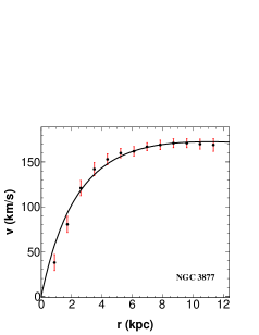
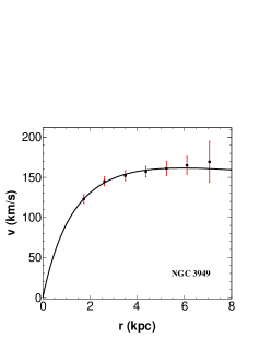
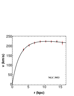
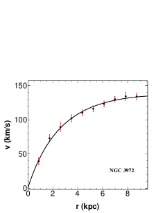
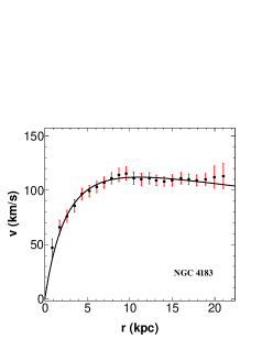
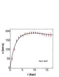
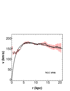
Figure 1: Fitting of equation (32) for the new $f(\mathcal{R})$ gravity model (29) to the rotational velocities (in km/s) of a set of nine HSB galaxies extracted from Ref. mannheim with their errors plotted as a function of radial distance (in kpc).

V.1 Analysis of HSB galaxy sample

We fit the predictions of the new $f(\mathcal{R})$ gravity model (29) as obtained from equation (32) to the data of a sample of nine HSB galaxies extracted from Ref. mannheim . In these fittings and subsequent ones we use the $\chi^{2}$ minimization technique. Table 1 shows the related data for the nine HSB galaxies along with the respective best fit values of the parameters $M_{0}$ and $r_{c}$ and the reduced chi-squared ($\chi_{red}^{2}$) values. The results are depicted in Fig. 1.

In Table 1, the data of HI gas mass $M_{HI}$ (which extends well beyond the optical disk distributions) in units of $10^{10}M_{\odot}$, the disk scale length $R_{0}$ measured in units of kpc, the adopted distance $D$ in Mpc and the B-band luminosity in units of $10^{10}L_{\odot}$ are extracted from Ref mannheim . The total gas mass is given by $\frac{4}{3}M_{HI}$ capistrano ; sporea ; mannheim ; karukes and the stellar mass is obtained by subtracting the gas mass from the predicted total mass of the galaxy. We have also listed the stellar mass-to-light ratios $(M/L)_{\ast}$. It is seen that in almost all the cases, the mass-to-light ratios inferred from the fit are reasonably close to the expected mass-to-light ratios. One should note that the expected mass-to-light ratios of galaxies lie within the range of $0.2\,M_{\odot}/L_{\odot}<M/L<10\,M_{\odot}/L_{\odot}$ sanders . Also, Fig. 1 depicts that almost all of the selected galaxies are well-fitted by the recently proposed $f(\mathcal{R})$ model (29), except the galaxy NGC $6946$ for which the $\chi_{red}^{2}$ value is very large, around $15.13$. However, as one can see from Fig. 1, the shape of its rotation curve was not affected.

Table 2: Relevant galaxy properties for a set of 21 LSB galaxies and the best fit values for the parameters $M_{0}$ and $r_{c}$ of these galaxies in the new $f(\mathcal{R})$ gravity model (29).

Galaxy	Distance	$L_{B}$	$R_{0}$	$M_{HI}$	$M_{0}$	$r_{c}$	$\chi_{red}^{2}$	$(M/L)_{\ast}$
	$D$ (Mpc)	$(10^{10}L_{\odot})$	(kpc)	$(10^{10}M_{\odot})$	$(10^{10}M_{\odot})$	(kpc)		$({M_{\odot}}/{L_{\odot}})$
DDO 0064	6.8	0.015	1.3	0.02	0.209	0.84	0.63	12.15
F563-1	46.8	0.140	2.9	0.29	3.365	2.09	0.53	21.27
F563-V2	57.8	0.266	2.0	0.20	1.917	1.34	0.12	6.20
F568-3	80.0	0.351	4.2	0.30	2.100	2.66	0.38	4.84
F583-1	32.4	0.064	1.6	0.18	14.398	2.24	0.34	221.21
NGC 0055	1.9	0.588	1.9	0.13	10.976	2.35	1.22	16.01
NGC 0300	2.0	0.271	2.1	0.08	2.394	1.65	2.04	8.44
NGC 2976	3.6	0.201	1.2	0.01	0.945	0.84	1.42	4.63
NGC 3109	1.5	0.064	1.3	0.06	3.410	1.52	2.78	52.03
NGC 3917	16.9	1.334	2.8	0.17	7.774	2.26	0.42	5.65
UGC 1281	5.1	0.017	1.6	0.03	0.950	1.34	0.13	53.54
UGC 5005	51.4	0.200	4.6	0.28	13.277	4.43	0.34	64.52
UGC 5750	56.1	0.472	3.3	0.10	9.703	3.56	0.07	20.27
UGC 5999	44.9	0.170	4.4	0.18	6.468	3.57	0.09	36.64
UGC 6399	18.7	0.291	2.4	0.07	1.269	1.62	0.21	4.04
UGC 6667	19.8	0.422	3.1	0.10	0.548	1.60	0.65	0.98
UGC 6818	21.7	0.352	2.1	0.16	8.677	2.46	1.69	24.04
UGC 6923	18.0	0.297	1.5	0.08	1.005	1.11	0.65	3.02
UGC 6983	20.2	0.577	2.9	0.37	1.287	1.67	1.11	1.37
UGC 7089	13.9	0.352	2.3	0.07	2.013	1.92	0.85	5.45
UGC 11557	23.7	1.806	3.0	0.25	2.043	2.18	0.18	0.95

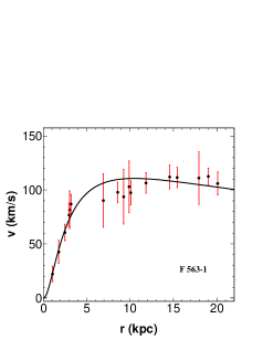
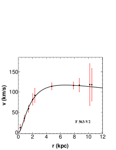
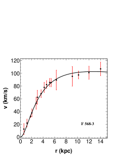
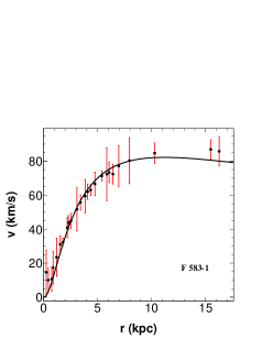
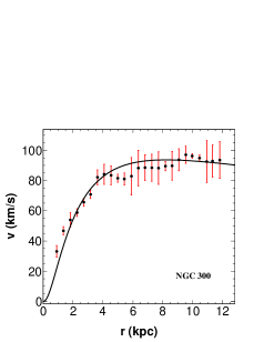
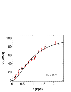
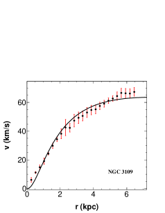
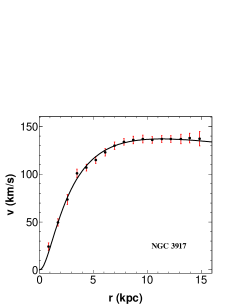
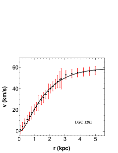
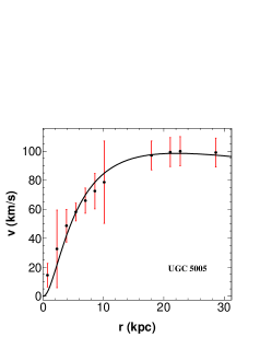
Figure 2: Fitting of equation (32) for the new model (29) to the rotational velocities (in km/s) of a set of 12 LSB galaxies extracted from Ref. mannheim with their errors plotted as a function of radial distance (in kpc).

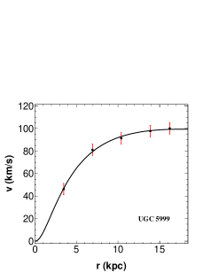
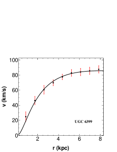
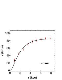
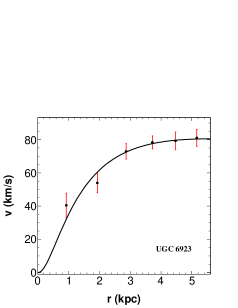
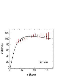
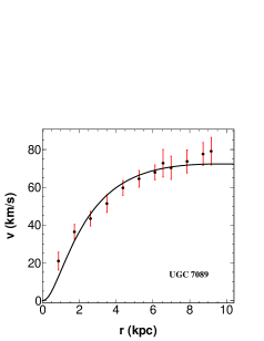
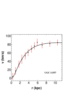
Figure 3: Fitting of equation (32) for the new model (29) to the rotational velocities (in km/s) of a set of 9 LSB galaxies extracted from Ref. mannheim with their errors plotted as a function of radial distance (in kpc).

Table 3: Relevant galaxy properties for a set of nine Dwarf galaxies and the best fit values for the parameters $M_{0}$ and $r_{c}$ of these galaxies in the new $f(\mathcal{R})$ gravity model (29).

Galaxy	Distance	$L_{B}$	$R_{0}$	$M_{HI}$	$M_{0}$	$r_{c}$	$\chi_{red}^{2}$	$(M/L)_{\ast}$
	$D$ (Mpc)	$(10^{9}L_{\odot})$	(kpc)	$(10^{9}M_{\odot})$	$(10^{9}M_{\odot})$	(kpc)		$({M_{\odot}}/{L_{\odot}})$
UGC 4325	11.87	1.71	1.92	1.04	1.612	0.79	0.25	0.132
UGC 4499	12.80	1.01	1.46	1.15	24.323	1.43	0.64	22.56
UGC 5414	9.40	0.49	1.40	0.57	6.257	1.08	1.08	11.22
UGC 7232	3.14	0.08	0.30	0.06	3.222	0.33	0.86	39.27
UGC 7323	7.90	2.39	2.13	0.70	16.275	1.59	2.75	6.41
UGC 7524	4.12	1.37	3.02	1.34	9.921	1.90	2.13	5.94
UGC 7559	4.20	0.04	0.87	0.12	1.279	0.69	0.16	27.99
UGC 7577	3.03	0.10	0.73	0.06	0.895	0.73	0.17	8.15
UGC 12632	9.20	0.86	3.43	1.55	3.487	1.68	0.75	1.65

V.2 Analysis of LSB galaxy sample

It is well known that LSB galaxies are regarded as dark matter dominated galaxies and hence, they can provide a satisfactory test for a gravitational theory deblok2002 ; mannheim . To this end, we fit equation (32) to a sample of 21 LSB galaxies extracted from Ref. mannheim with their maximum radial distance varying from $2.1$ kpc to $18.2$ kpc. Table 2 compiles the relevant data for these galaxies we have selected from the $111$ galaxies studied in Ref. mannheim along with the respective best fit values of the parameters $M_{0}$ and $r_{c}$ and the $\chi_{red}^{2}$ values of the fits. The results are presented in Fig. 2 and 3.

It is seen from Table 2 that the mass-to-light ratios for few galaxy samples are much larger than the upper bound $10({M_{\odot}}/{L_{\odot}})$ sanders . However, as can be seen from Figs. 2 and 3, the rotation curves are well fitted with the observed data as the $\chi_{red}^{2}$ values are smaller than or equivalent to $1$ for almost all of the galaxies in the sample. For the galaxies NGC $0300$, NGC $3109$ and UGC $6818$ although the $\chi_{red}^{2}$ values are high, around $2.04$, $2.78$ and $1.69$ respectively, these do not affect the shape of the fitted rotation curves.

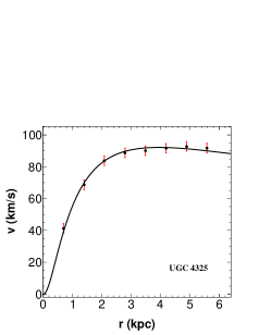
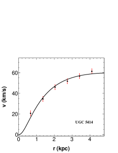
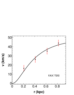
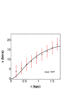
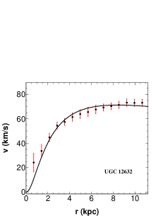
Figure 4: Fitting of equation (32) for the new model (29) to the rotational velocities (in km/s) of a set of nine dwarf galaxies extracted from Ref. mannheim with their errors plotted as a function of radial distance (in kpc).

V.3 Analysis of dwarf galaxy sample

For dwarf galaxies, we have chosen a sample of nine galaxies taken from Ref. obrien . Table 3 compiles the relevant data for the chosen galaxy sample and the results are depicted in Fig. 3. For all the galaxies the $\chi_{red}^{2}$ values are small and gives well fitted galactic rotation curves, except for two galaxies viz., UGC $7323$ and UGC $7524$. Furthermore, the mass-to-light ratio for most of the galaxies are within the upper bound. However, for two galaxies namely, UGC $4499$ and UGC $7559$, the mass-to-light ratios are notably greater than the upper bound value as expected from the population synthesis models sanders . According to the population synthesis models depending on the history of the star formation and also on metallicities the blue-band mass-to-light ratio may range from a few tenths to 10.

V.4 Analysis of an ultra diffuse galaxy

Here, we analyze the rotation curve of an ultra diffuse galaxy (UDG), AGC $242019$, which was identified by the Arecibo Legacy Fast ALFA (ALFALFA) survey of HI galaxies leisman . This galaxy has an HI mass of $8.51\times 10^{8}$ M_⊙ and a corresponding distance of $30.8$ Mpc. The gas rich UDG AGC $242019$ has been claimed to be like an observed LSB galaxy with a slowly rising rotation curve shi21 . Fig. 4 shows the fitted rotation curve with the data taken from Ref. shi21 . It can be seen that the curve of this galaxy is well fitted with observation. In fact, from Fig. 4 one can see that the rotation curve is slowly rising, indicating that UDG AGC $242019$ can be considered as a member of a class of LSB galaxies. However, further study in this regard is still required to confirm such proclamation. From our study, the $\chi_{red}^{2}$ value is obtained as $6.84$ and the fitted parameters are evaluated to be $M_{0}=4.92$ ($10^{10}M_{\odot}$) and $r_{c}=2.29$ (kpc). Thus, the flat rotation curve of UDG AGC $242019$ can be explained via the new model (29) of $f(\mathcal{R})$ gravity.

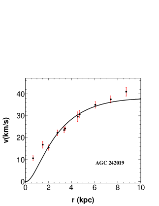
Figure 5: The rotational velocities of AGC $242019$ fitted to equation (32) with the associated errors plotted as a function of radial distance in kpc. The data for the rotational velocities of the galaxy is taken from Ref. shi21 .

VI The Tully-Fisher relation

R. B. Tully and J. R. Fisher in 1977 published a method of determining the distances of spiral galaxies based on their empirical or observational relation, now known as the Tully-Fisher relation tully . It implies a relation between the luminosity of a galaxy and the velocity of the outermost observed point of the galaxy as

$$L=\xi\,v_{out}^{a},$$ (34)

where $L$ is the observed luminosity of a galaxy in units of $10^{10}L_{\odot}$, $v_{out}$ is the velocity at the outermost observed radial point of the galaxy in units of km/s, $\xi$ is the proportionality constant and $a$ is another constant. Taking logarithm on both sides of this equation (34), we may write

$$\log L=a\log v_{out}+b.$$ (35)

Here $b=\log\xi$. We plotted the observed Tully-Fisher relation for the entire samples of galaxies used in this study as shown in the left panel of Fig. 5. In the plot the vertical axis is the base $10$ logarithm of the $B$-band luminosity $L_{B}$ in units of $10^{10}L_{\odot}$ and the horizontal axis is the base $10$ logarithm of the velocity of the outermost observed radial point in units of kms^-1. The $B$-band luminosity data for each galaxy sample has been extracted from Ref. mannheim and are tabulated in Tables 1, 2 and 3. The solid line in the plot is the best least-square fitting of equation (35) to the observed corresponding data of galaxies as mentioned. The fitting is found to be very good with $\chi^{2}_{red}=0.127$ and the parameters $a=3.18\,\pm\,0.27$ and $b=-\,6.75\,\pm\,0.54$.

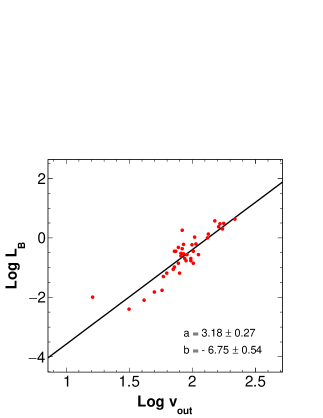
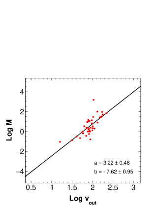
Figure 6: Plots for the Tully-Fisher relation. The left panel is for the observed $B$ band Tully-Fisher relation. The line in the plot is obtained by fitting equation (35) to the observed data. The right panel shows predicted Tully-Fisher relation for the masses and velocities of the outermost radial points of galaxies predicted from the new $f(\mathcal{R})$ model (29). Here the solid line represents the best least-square fitting of (36) to the corresponding predicted data as mentioned.

Now, from the mean mass-luminosity relation $\langle M/L\rangle=constant$ brownstein and equation (35) we can write the Tully-Fisher relation in terms of the predicted mass (in units of $10^{10}M_{\odot}$) and the velocity (in units of kms^-1 for the new $f(\mathcal{R})$ gravity model (29) as

$$\log M=a\log v+b+\log\langle M/L\rangle.$$ (36)

The right panel of Fig. 5 shows the best fit Tully-Fisher relation parametrized by equation (36) for the new model (29). The vertical axis denotes the base $10$ logarithm of the predicted mass (in units of $10^{10}M_{\odot}$) and the horizontal axis denotes the base $10$ logarithm of the fitted velocity (in units of kms^-1). In this fit the parameters are found to be $a=3.22\,\pm\,0.48$ and $b=-\,7.62\,\pm\,0.95$ with $\chi^{2}_{red}=0.397$.

VII Summary and final remarks

The behaviour of galactic rotation curves indicates the need for DM or some modifications of GR. However, till date there is no direct evidence of the existence of DM. Also, DM interacts only via gravity and hence, the question arises as to whether the effect of DM is a consequence of the modification of gravity only. Keeping this point in mind, in this work, we have employed one of the simplest MTG, the $f(\mathcal{R})$ gravity to study the galactic rotation curves for some of the galaxies observed experimentally in recent times. In doing so we have mainly tried to test the viability of the recently proposed model dhruba ; Dhruba of $f(\mathcal{R})$ gravity in the galactic scales.

In our present work, we have used the Palatini formalism along with the Weyl transformation. Thus the variation of the action for the $f(\mathcal{R})$ theory first with respect to the metric and then with respect to the connection yields the field equations in the theory. We consider the Weyl transformation which is the frame transformation of the spacetime metric $g_{\mu\nu}$ from the Jordan frame to the Einstein frame to get the field equation in the convenient form of GR. Moreover, the connection in this torsion-free Palatini approach is the Levi-Civita connection for the conformally related metric and as such particles moving in the gravitational field follow the geodesics obtained by the connection. In the Einstein frame, we study the rotational velocity of a test particle moving in a stable circular orbit. A static spherically symmetric metric is taken into consideration and we are able to derive the co-efficients of the metric for our galactic model spacetime.

Next, we introduce the new model of $f(\mathcal{R})$ gravity. As mentioned already this is a recently introduced $f(\mathcal{R})$ gravity model and hence we try to test the viability of this model in the galactic scales. Making use of the metric co-efficients and the field equations we derive the analytical expression for rotational velocities of test particles in the stable circular orbits. It can be observed that the expression of the rotational velocity obtained is different from the Newtonian one. This is due to the fact that the rotational velocity obtained via our present approach has extra terms coming from the geometrical modifications in the theory. This rotational velocity expression is fitted with observed data of a few samples of galaxies. We consider nine samples of high surface brightness (HSB) galaxies, 21 samples of low surface brightness (LSB) galaxies and nine dwarf galaxies. The galactic rotation curves are well fitted with observations for the new $f(\mathcal{R})$ gravity model. Although, for a few samples of galaxies the mass-to-light ratios are found to be much larger than the expected upper bound, however the $\chi_{red}^{2}$ values for most of the samples are smaller or equivalent to 1, thus indicating the well fitted rotation curves. This shows the viability of the new $f(\mathcal{R})$ gravity model in the galactic scales.

In addition to these samples, we take into consideration an interesting class of galaxies i.e., the ultra diffuse galaxies (UDGs). They are fascinating objects which are either made entirely of DM or have a high content of DM. This makes them difficult to observe and analyze. We consider one such galaxy, AGC $242019$, which has been claimed to be similar to low surface brightness galaxies with a slowly rising rotation curve. Our study supports this proclamation. However, further studies are necessary in this regard.

Finally, we have studied the Tully-Fisher relation in the new $f(\mathcal{R})$ gravity model. We have studied the luminosity as well as total mass of galaxies as a function of velocity of the outermost observed radial point. The entire sample of galaxies have been combined for this purpose and the fits show a consistent result across the galaxies. In our work, we have made use of the SPARC catalogue (http://astroweb.cwru.edu/SPARC/) for the observational data of the sample of galaxies.

Lastly, it would be interesting to extend our work by including different MTGs with more observational data and also by comparing our results with the standard DM profiles such as Navarro-Frenk-White (NFW) nfw ; navarro and Burkert burkert profiles. Also, in the near future, we can try to obtain much feasible mass-to-light ratios within the expected bound.

References

- (1) G. Bertone and D. Hooper, Rev. Mod. Phys. 90, 045002 (2018) [arXiv:1605.04909].
- (2) J. G. de Swart, G. Bertone and J. van Dongen, Nature Astron. 1, 0059 (2017) [arXiv:1703.00013].
- (3) G. Bertone and T. M. P. Tait, Nature 562, 51-56 (2018) [arXiv:1810.01668].
- (4) C. S. Frenk and S. D. M. White, Ann. Phys. (Berlin), 507534 (2012) [arXiv:1210.0544].
- (5) L. E. Strigari, Phys. Rep. 531, 1-88 (2013) [arXiv:1211.7090].
- (6) J. H. Oort, Bull. Astron. Inst. the Netherlands. 6, 249 (1932).
- (7) F. Zwicky, Helv. Phys. Acta. 6, 110-127 (1933); F. Zwicky, Gen. Relativ. Gravit. 41, 207224 (2009).
- (8) F. Zwicky, Astrophys. J. 86, 217-246 (1937).
- (9) V. C. Rubin, N. Thonnard and W. K. Ford Jr., Astrophys. J. 238, 471-487 (1980).
- (10) Bing-Lin Young, Front. Phys. 12, 121201 (2017).
- (11) A. Borriello and P. Salucci, Mon. Not. R. Astron. Soc. 323, 285-292 (2001) [arXiv:astro-ph/0001082].
- (12) R. Massey, T. Kitching and J. Richard, Rep. Prog. Phys. 73, 086901 (2010) [arXiv:1001.1739].
- (13) K. Garrett and G. Dūda, Adv. Astron., 968283 (2011) [arXiv:1006.2483].
- (14) P. A. R. Ade, et al., Astron. Astrophys. 594, A13 (2016) [arXiv:1502.01589].
- (15) G. Bertone, D. Hooper and J. Silk, Phys. Rep. 405, 279-390 (2005) [arXiv:hep-ph/0404175].
- (16) J. L. Feng, Ann. Rev. Astron. Astrophys. 48, 495-545 (2010) [arXiv:1003.0904].
- (17) A. G. Riess et al., Astron. J. 116, 1009-1038 (1998) [arXiv:astro-ph/9805201].
- (18) S. Perlmutter et al., Astrophys. J. 517, 565-586 (1999) [arXiv:astro-ph/9812133].
- (19) T. Clifton, [arXiv:gr-qc/0610071].
- (20) R. V. Wagoner, Phys. Rev. D 1, 3209 (1970).
- (21) R. W. Hellings and K. Nordtvedt, Jr., Phys. Rev. D 7, 3593 (1973).
- (22) S. Alexander and N. Yunes, Phys. Rev. D 75, 124022 (2007) [arXiv:0704.0299].
- (23) J. Alsing et al., Phys. Rev. D, 85, 064041 (2012) [arXiv:1112.4903].
- (24) Alan H. Guth, Phys. Rev. D 23, 347-356 (1981).
- (25) S. Capozziello and M. De Laurentis, Phys. Rep. 509, 167-321 (2011) [arXiv:1108.6266].
- (26) T. Clifton et al., Phys. Rep. 513, 1-189 (2012) [arXiv:1106.2476].
- (27) S. Nojiri, S.D. Odintsov and V.K. Oikonomou, Phys. Rept. 692, 1-104 (2017) [arXiv:1705.11098].
- (28) S. Nojiri and S.D. Odintsov, Phys. Rept. 505, 59-144 (2011) [arXiv:1011.0544].
- (29) S. Nojiri and S.D. Odintsov, TSPU Bulletin N 8(110), 7 (2011) [arXiv:0807.0685].
- (30) T. P. Sotiriou and V. Faraoni, Rev. Mod. Phys. 82, 451 (2010) [arXiv:0805.1726].
- (31) A. De Felice and S. Tsujikawa, Living Rev. Rel. 13, 3 (2010) [arXiv:1002.4928].
- (32) R. Zaregonbadi, M. Farhoudi and N. Riazi, Phys. Rev. D 94, 084052 (2016) [arXiv:1608.00469].
- (33) Y. Shtanov, Phys. Lett. B 820, 136469 (2021) [arXiv:2105.02662].
- (34) N. Parbin and U. D. Goswami, Mod. Phys. Lett. A 36, 2150265 (2021) [arXiv:2007.07480].
- (35) C. G. Böhmer, T. Harko and F. S. N. Lobo, Astropart. Phys. 29, 386-392 (2008) [arXiv:0709.0046].
- (36) Y. Shtanov, [arXiv:2207.00267].
- (37) T. Katsuragawa and S. Matsuzaki, Phys. Rev. D 95, 044040 (2017) [arXiv:1610.01016].
- (38) F. S. N. Lobo, Dark Energy-Current Advances and Ideas, 173-204 (2009) [arXiv:0807.1640].
- (39) T. Harko, Phys. Rev. D 81, 084050 (2010) [arXiv:1004.0576].
- (40) T. P. Sotiriou and S. Liberati, Annals of Physics 322, 935 (2007).
- (41) S. Capozziello et al., Astropart. Phys. 50-52, 65-75 (2013) [arXiv:1307.0752].
- (42) L. Á. Gergely et al., Mon. Not. R. Astron. Soc. 415, 3275-3290 (2011) [arXiv:1105.0159].
- (43) V. F. Cardone et al., Mon. Not. R. Astron. Soc. 423, 141-148 (2012) [arXiv:1202.2233].
- (44) C. A. Sporea, A. Borowiec and A. Wojnar, Eur. Phys. J. C 78, 308 (2018) [arXiv:1705.04131].
- (45) A. Finch and J. L. Said, Eur. Phys. J. C 78, 560 (2018) [arXiv:1806.09677].
- (46) Hai-Nan Lin et al., MNRAS 430, 450-458 (2013) [arXiv:1209.3532].
- (47) S. Capozziello, V. F. Cardone and A. Troisi, Mon. Not. R. Astron. Soc. 375, 1423-1440 (2007) [arXiv:astro-ph/0603522].
- (48) P. Salucci, C. F. Martins and E. Karukes, Int. J. Mod. Phys. D 23, 1442005 (2014) [arXiv:1405.6314].
- (49) C. F. Martins and P. Salucci, Mon. Not. R. Astron. Soc. 381, 1103-1108 (2007) [arXiv:astro-ph/0703243].
- (50) V. K. Sharma, B. K. Yadav and M. M. Verma, Eur. Phys. J. C 80, 619 (2020) [arXiv:1912.12206].
- (51) U. D. Goswami and K. Deka, Int. J. Mod. Phys. D 22, 1350083 (2013) [arXiv:1303.5868].
- (52) S. Capozziello, F. Darabi and D. Vernieri, Mod. Phys. Lett. A 25, 3279-3289 (2010) [arXiv:1009.2580].
- (53) Y. Shtanov, Universe 8(2), 69 (2022) [arXiv:2202.00818].
- (54) G. J. Olmo, Int. J. Mod. Phys. D 20, 413-462 (2011) [arXiv:1101.3864].
- (55) D. J. Gogoi and U. D. Goswami, Eur. Phys. J. C 80, 1101 (2020) [arXiv:2006.04011].
- (56) D. J. Gogoi and U. D. Goswami, IJMP D 31, 2250048 (2022) [arXiv:2108.01409].
- (57) P. van Dokkum et al., ApJL 828, L6 (2016) [arXiv:1606.06291].
- (58) P. van Dokkum et al., Nature 555, 629-632 (2018) [arXiv:1803.10237].
- (59) G. D. Bothun, C. Impey and F. D. Malin, ApJ 376, 404 (1991).
- (60) G. Bothun, C. Impey and S. Mcgaugh, PASP 109, 745 (1997).
- (61) P. van Dokkum et al., ApJ 798, L45 (2015) [arXiv:1410.8141].
- (62) J. Román and I. Trujillo, MNRAS 468, 703-716 (2017) [arXiv:1603.03494].
- (63) T. Ruiz-Lara et al., MNRAS 478, 2034-2045 (2018) [arXiv:1803.06298].
- (64) D. A. Forbes et al., MNRAS 500, 1279-1284 (2021) [arXiv:2010.07313].
- (65) C. B. Brook et al., ApJL 919, L1 (2021) [arXiv:2109.01402].
- (66) Yong Shi et al., ApJ 909, 20 (2021) [arXiv:2101.01282].
- (67) R. B. Tully and J. R. Fisher, Astron. Astrophys. 54, 661-673 (1977).
- (68) J. R. Brownstein and J. W. Moffat, ApJ 636, 721-741 (2006) [arXiv:astro-ph/0506370].
- (69) S. S. Mcgaugh et al., ApJ 533, L99-L102 (2000) [arXiv:astro-ph/0003001].
- (70) J. Bora et al., [arXiv:2204.05473].
- (71) J. Binney and S. Tremaine, Galactic Dynamics, nd Edn. (Princeton University Press, Princeton, 2008).
- (72) V. D. Sandberg, Phys. Rev. D 12, 3013 (1975).
- (73) C. W. Misner, S. Thorne and J. A. Wheeler, Gravitation, (W. H. Freeman and Co., NY, 1973).
- (74) S. Capozziello, F. S. N. Lobo and J. P. Mimoso, Phys. Rev. D 91, 124019 (2015) [arXiv:1407.7293].
- (75) A. Wojnar and H. Velten, Eur. Phys. J. C 76, 697 (2016) [arXiv:1604.04257].
- (76) S. Weinberg, Gravitation and cosmology: principles and applications of the general theory of relativity, st Edn. (Wiley, Hoboken, 1972).
- (77) P. D. Mannheim and J. G. O’Brien, Phys. Rev. D 85, 124020 (2012) [arXiv:1011.3495].
- (78) A. J. S. Capistrano and G. R. G. Barrocas, MNRAS 475, 2204-2214 (2018).
- (79) E. V. Karukes and P. Salucci, MNRAS 465, 4703-4722 (2017) [arXiv:1609.06903].
- (80) W. J. G. de Blok and A. Bosma, Astron. Astrophys. 385, 816-846 (2002) [arXiv:astro-ph/0201276].
- (81) R. H. Sanders, ApJ 473, 117 (1996) [arXiv:astro-ph/9606089].
- (82) J. G. O’Brien and P. D. Mannheim, Mon. Not. R. Astron. Soc. 421, 1273-1282 (2012) [arXiv:1107.5229].
- (83) L. Leisman, ApJ 842, 133 (2017) [arXiv:1703.05293].
- (84) J. F. Navarro, C. S. Frenk and S. D. M. White, Astrophys. J 462, 563-575 (1996) [arXiv:astro-ph/9508025].
- (85) J. F. Navarro, C. S. Frenk and S. D. M. White, Astrophys. J 490, 493 (1997) [arXiv:astro-ph/9611107].
- (86) A. Burkert, Astrophys. J 447, L25 (1995) [arXiv:astro-ph/9504041].