Finding Point with Image: A Simple and Efficient Method for UAV Self-Localization

Abstract

Image retrieval has emerged as a prominent solution for the self-localization task of unmanned aerial vehicles (UAVs). However, this approach involves complicated pre-processing and post-processing operations, placing significant demands on both computational and storage resources. To mitigate this issue, this paper presents an end-to-end positioning framework, namely Finding Point with Image (FPI), which aims to directly identify the corresponding location of a UAV in satellite-view images via a UAV-view image. To validate the practicality of our framework, we construct a paired dataset, namely UL14, that consists of UAV and satellite views. In addition, we establish two transformer-based baseline models, Post Fusion and Mix Fusion, for end-to-end training and inference. Through experiments, we can conclude that fusion in the backbone network can achieve better performance than later fusion. Furthermore, considering the singleness of paired images, Random Scale Crop (RSC) is proposed to enrich the diversity of the paired data. Also, the ratio and weight of positive and negative samples play a key role in model convergence. Therefore, we conducted experimental verification and proposed a Weight Balance Loss (WBL) to weigh the impact of positive and negative samples. Last, our proposed baseline based on Mix Fusion structure exhibits superior performance in time and storage efficiency, amounting to just 1/24 and 1/68, respectively, while delivering comparable or even superior performance compared to the image retrieval method. The dataset and code will be made publicly available.

I Introduction

In recent years, the application of vision-related missions for unmanned aerial vehicles (UAVs) has become widespread across various fields [1, 2, 3], including facility inspection, agricultural operations, ground reconnaissance, civilian aerial photography, etc. While UAVs typically rely on Global Positioning System (GPS) signals for self-localization. However, the stability of these signals can vary in different scenarios. UAVs often operate in environments where GPS signals are weak or entirely unavailable. In such cases, the UAVs will face the consequences of not working properly or even losing control. This paper aims to investigate a self-localization task for UAVs merely based on visual information, offering an alternative positioning method in GPS-denial environments.

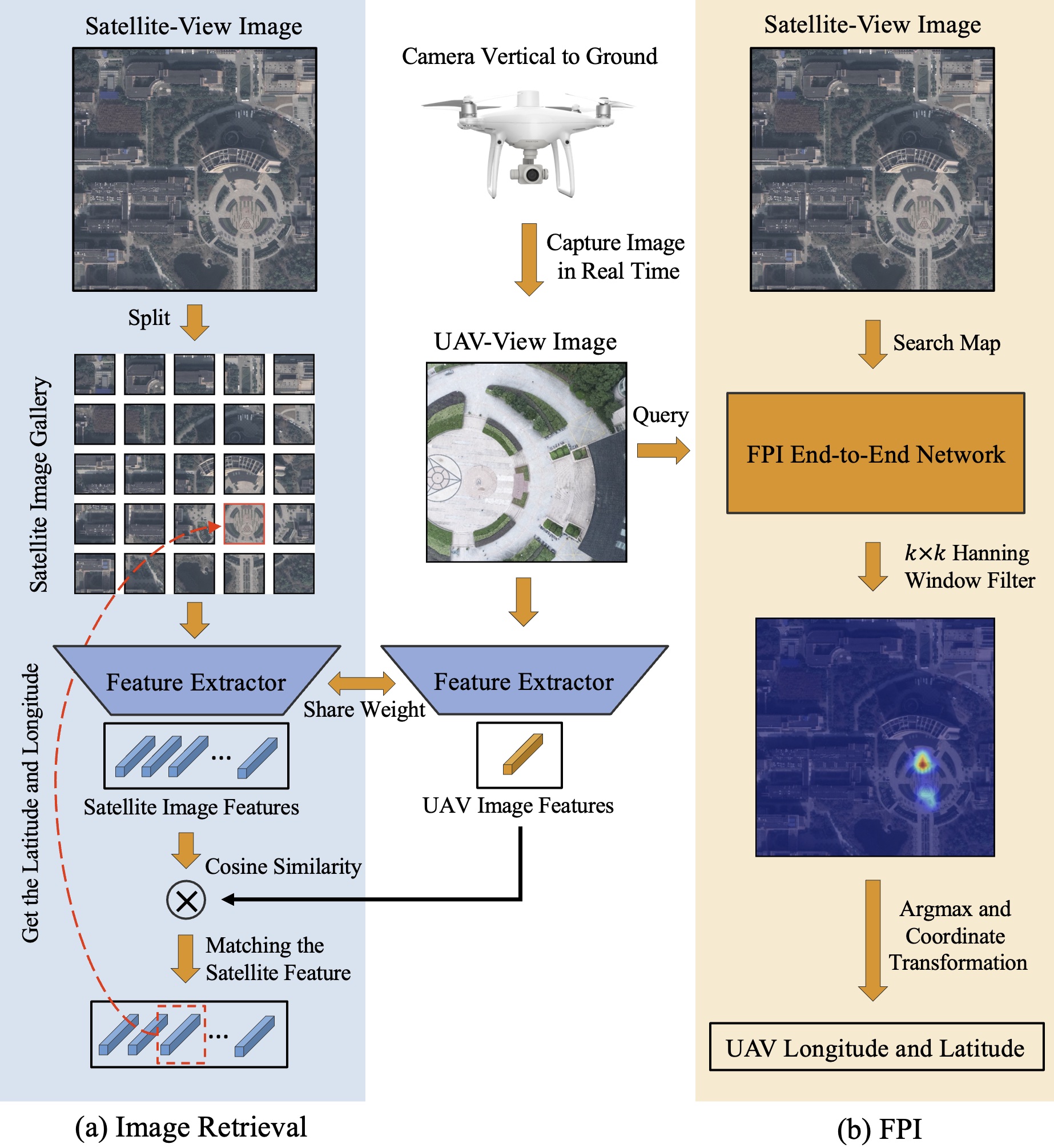
Figure 1: A comparison between (a) image retrieval and (b) the proposed FPI framework for UAV self-localization.

For conventional positioning tasks, feature point matching methods like Scale-Invariant Feature Transform (SIFT) [4] and Speeded-Up Robust Features (SURF) [5] are commonly employed. These methods utilize hand-designed feature descriptors that possess advantageous properties such as scale, rotation, and invariance. They have been successfully and widely used in Simultaneous Localization And Mapping (SLAM)[6] and Image Stitching[7] tasks. However, when it comes to scenarios where the image quality varies significantly between domains, the corner-point pairing approach can only make use of a limited number of distinctive features. As a result, its effectiveness is considerably diminished. To overcome these challenges, deep learning has gained prominence as it can exploit richer associations between features and deliver superior performance in such demanding tasks.

The UAV self-localization task presents several challenges, including domain differences, inconsistent viewing angles and spatial information due to time offsets. Thus, some deep learning methods have been developed to improve content understanding and feature integration. One such method is DenseUAV [8], which adopted an image retrieval scheme and used the UAV-view image as a query to retrieve the most similar satellite-view image from a satellite gallery. Subsequently, GPS information is obtained to determine the UAV’s position. Although it significantly improves positioning accuracy, it incurs high costs on the application side. Specifically, we elaborate on the inference implications associated with image retrieval as illustrated in Fig. 1 (a). First, it is necessary to split the relatively large-scale satellite-view images to generate the satellite image gallery. In most cases, the machine’s operating memory is insufficient to accommodate the entire gallery. Therefore, we need to store the satellite image gallery on disk temporarily. Following that, the entire gallery is subjected to feature extraction by a neural network feature extractor, and the features also need to be stored on disk. The above steps constitute the pre-processing part of the image retrieval solution, and its time and space complexity are directly proportional to the size of the gallery. The pre-processing part essentially prepares a feature library for retrieval in advance, although the process is complex, it does not affect the real-time performance of UAV self-localization. Actually, the UAV captures real-time images from the camera facing vertically toward the ground, and similarly, the UAV image features are extracted by the feature extractor. These features are then used to compute the cosine similarity with the satellite features. Last, we obtain the GPS position information corresponding to the satellite feature that best matches.

Given the complex pre- and post-processing of image retrieval schemes, this paper aims to explore a more straightforward way for UAV self-localization. To this end, we propose the end-to-end Finding Point with Image (FPI) architecture that uses multi-source data as the input. For simplicity, we refer to the UAV image as query and the satellite image as search map. For FPI, the query and search map are directly fed into the network, which outputs a heatmap representing the predicted probability distribution of the query’s location in the search map, as illustrated in Fig. 1 (b). Different from image retrieval, FPI does not require extensive preparatory data and feature extraction operations beforehand. The only thing that needs to be prepared and saved is a large satellite image. The pre-process has been greatly simplified. Then, it only needs to input the real-time images acquired by the UAV and the dynamically cropped satellite images into the FPI model, and a response heatmap of the UAV’s position probability can be directly output. In order to filter out noise points, we additionally added $k\times{k}$ hanning window filter. Last, we obtain the maximum thermal response position through the argmax operation and calculate the longitude and latitude coordinates of the UAV through coordinate transformation.

Compared with image retrieval, the advantages of FPI can be summarized as follows. 1) Simplified localization process. FPI eliminates the need for pre-building a satellite gallery and avoids complex post-processing. 2) High potential for localization accuracy. FPI overcomes the inherent localization errors caused by sampling intervals, and the localization accuracy is solely determined by the model itself. This presents the potential for achieving higher localization precision. 3) Faster inference. FPI eliminates the need for calculating cosine similarity with features in the gallery. The inference speed is determined solely by the model, resulting in more efficient localization. 4) Localization anytime and anywhere. Just prepare a satellite image in advance. 5) Flexible model updates. Only the model needs to be replaced when the model is iteratively updated. The details will be compared in Section V-B.

The main research content of this paper is to explore a simple and effective end-to-end architecture FPI to implement UAV self-localization tasks. However, in addition to the architecture, we did some additional detailed exploration to help researchers analyze the task. At the same time, we have done a lot of experimental research from the data and model levels to provide some references for researchers. Specifically, considering the needs of FPI training, we reconstructed the dataset UL14, and based on it, proposed two model architectures called Post Fusion (FPI-PF) and Mix Fusion (FPI-MF). Additionally, we design two additional evaluation metrics: Meter-level Accuracy (MA), which provides an intuitive measurement of spatial distance, and Relative Distance Score (RDS), which assesses the positioning performance at the model level to comprehensively evaluate the performance of this task. Furthermore, we employ a data augmentation technique involving random scaling and random offset to enrich the combination of training sample pairs. Moreover, we introduce negative sample weight factor on the basis of balance loss, which effectively improves the training process and contributes to overall model optimization.

The main contributions can be listed as follows:

• We propose a simple and efficient UAV self-localization architecture called Find Point with Image (FPI), which does not require additional pre- and post-processing operations, thus improving the efficiency of the application.

• We constructed a new benchmark, which includes a new dataset UL14 constructed from paired samples, and evaluation indicators Meter-level Accuracy (MA) and Relative Distance Score (RDS).

• We present two model architectures, Post Fusion and Mix Fusion to achieve UAV self-localization tasks, and conclude that the Mix Fusion is more effective than the Post Fusion. Moreover, we introduce a data augmentation technique involving random scale and offset to enrich the diversity of training data. Additionally, we improve balance loss and analyze the impact of the number and weight of positive and negative samples.

• The FPI architecture achieves comparable or even better accuracy than image retrieval while significantly improving inference speed and reducing storage consumption.

The remainder of this paper is structured as follows. First, we introduce the related work in Section II. Then, the model architecture of FPI is designed in Section III, and the proposed dataset and evaluation metrics are presented in Section IV. Next, we analyze the experiments from data-level and model-level in Section V and Section VI. Last, the visualization and conclusion are drawn in Section VII and Section VIII.

II Related Work

II-A Geo-Localization Dataset

II-A1 Ground-to-Aerial Matching

Geo-localization originally addressed the task of matching ground and aerial imagery. Some seminal investigations conducted by [9, 10, 11] laid the foundation for leveraging publicly available resources to establish image pairs encompassing ground and aerial views. Subsequently, the CVUSA[12] project devised image pairings derived from ground-based panoramic images and satellite imagery, whereas CVACT[13] further enhanced CVUSA by incorporating spatial elements, such as orientation maps. Recently, VIGOR[14] redefined the problem by adopting a more realistic assumption: that the query image can be of arbitrary nature within the specified area of interest.

II-A2 Drone-to-Satellite Matching

Univerisity-1652[15] introduced drone-view into cross-view geo-localization and proposed two drone-based subtasks: drone-view target localization and drone navigation, and regarded them as image retrieval tasks. SUE-200[16] improved the model’s adaptability to drone flight altitudes by collecting drone images at 4 different altitudes. Inspired by Univeristy-1652, DenseUAV[8] achieved high precision localization of UAVs by dense sampling, which is the first time to solve the vision-based UAV self-localization problem by the scheme of image retrieval.

II-B Deeply-Learned Geo-Localizatioin

Due to the potential applications, Cross-View Geo-Localization (CVGL) has gotten increased attention in recent years. Some pioneering methods[17, 18, 19, 20], concentrated on extracting hand-crafted features. Inspired by the powerful feature extraction capability of deep Convolutional Neural Networks (CNNs), most of the later works are carried out on the basis of deep learning [21, 22, 23, 24, 25]. Since drone-view was introduced for CVGL task, several methods have been proposed specifically for addressing the challenges in drone-view. DSM[26] took into account a limited field of view and employed a dynamic similarity matching module to align the orientation of cross-view images. PLCD[27] took advantage of drone-view information as a bridge between ground-view and satellite-view domains. LPN[28] proposed the square-ring partition strategy to allow the network to pay attention to more fine-grained information at the edge and achieved a huge improvement. FSRA[29] introduced a simple and efficient transformer-based structure to enhance the ability of the model to understand contextual information as well as to understand the distribution of instances.

II-C Single Object Tracking (SOT)

The idea of FPI is mainly inspired by algorithms in the field of SOT which deals with homogeneous data. However, the difference is that FPI deals with non-homogeneous input data. The UAV image in FPI is equivalent to the template for SOT, and the satellite map is the image containing the template.

Typically, most tracking methods are constructed based on a dual-stream architecture of siamese networks [30, 31, 32]. This type of method extracts features from two domains through a shared backbone network, and performs feature fusion through convolution operations. With the burgeoning development of Transformer technology in the field of computer vision, some feature fusion methods based on attention mechanisms have been introduced into the SOT domain[33, 34]. Recently, some single-stream frameworks are proposed, which introduces the interactive module into the backbone network to achieve deep feature fusion [35, 36].

II-D Transformer in Vision

In recent years, Transformer [37] has gradually become the mainstream basic model architecture in the fields of natural language processing (NLP)[38, 39] and computer vision (CV)[40, 41]. Some CVGL methods have also been further improved with the help of Transformer. Currently, the backbone based on the vision Transformer can be mainly divided into two categories. One is the unstructured Transformer structure, the most typical models such as ViT[40], and DeiT[41]. The other is the hierarchical Transformer structure, which typically includes PvT[42], CvT[43], and Swin-Transformer[44], which are widely used in fine-grained tasks such as object detection[45, 46] and image segmentation[47, 48].

Considering the requirements of this task for spatial context understanding and fine-grained mining capabilities. Through the experience of previous work [8] and the verification of our experiments, Transformer can perform better. More details will be analyzed in Section VI-D.

Figure 2: Structural diagram of the two structures of FPI, namely FPI-PF and FPI-MF. Post Fusion is a dual-stream architecture that interacts with drone and satellite image features through post-fusion. Mix Fusion is a single-stream network that interacts with feature information in the feature extraction part.

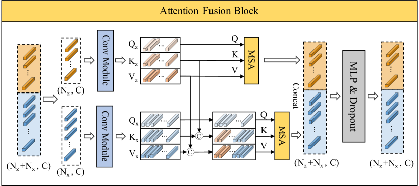
Figure 3: Structural diagram of Attention Fusion Block.

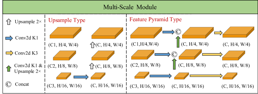
Figure 4: Structure diagram of two types of Multi-Scale Modules named Upsample and Feature Pyramid.

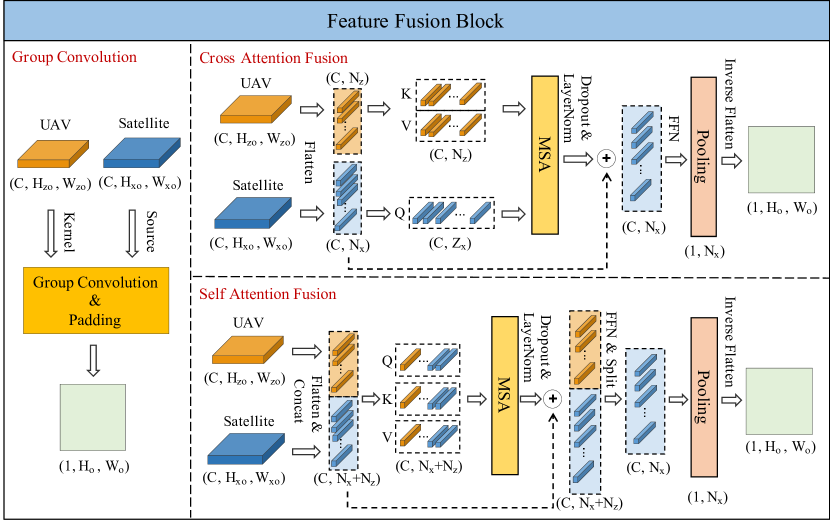
Figure 5: Structure diagram of three types of Feature Fusion Blocks named Group Convolution, Self Attention Fusion and Cross Attention Fusion.

III Methodology

III-A Localization Schemes

III-A1 Image Retrieval

This scheme determines image similarity by comparing feature similarity across domains, and then indirectly obtaining GPS information for localization. The detailed process is shown in Fig. 1(a). Although the retrieval-based scheme achieves good results in terms of positioning accuracy, it is not very flexible in practical application. Here lists several disadvantages of image retrieval in dealing with UAV self-localization tasks. 1) Complicated pre-processing: The interval of satellite image cropping directly determines the accuracy and speed of positioning, specifically, the denser the cut, the higher the positioning accuracy, but the slower the inference speed. 2) Intricate post-processing: The step of calculating feature similarity is a significant computational cost, and the amount of computation increases linearly with the increase in the satellite gallery. 3) Inflexible model iterability: Once the model is optimized, the feature gallery should be rebuilt. 4) Constrained geographical transferability: It cannot be located anytime and anywhere, and needs to pre-build a local feature gallery.

III-A2 Finding Point with Image (FPI)

The feature similarity calculation process of image retrieval can be likened to convolution operations, calculating feature correlation through a sliding window. Drawing inspiration from this and leveraging techniques from the SOT field which processes the same domain inputs, we propose a novel localization framework, named Finding Point with Image (FPI) to deal with UAV self-localization task. FPI distinguishes itself from image retrieval by eliminating the need for intricate pre- and post-processing steps, which aims to accomplish the UAV self-localization task by employing end-to-end inference with a single model. The steps involved in achieving positioning using the FPI scheme are shown in Fig. 1(b). FPI performs feature interaction, a fusion of the two sources, and finally outputs the heatmap of the spatial position. After simple processing such as hanning window filter and coordinate transformation, the position of the UAV can be obtained. FPI not only simplifies the self-localization task of the UAV in the process but also greatly improves the inference speed and storage resource consumption, which will be analyzed in detail in Section V-B

III-B Model Structure of FPI

III-B1 Post-Fusion (FPI-PF)

As illustrated in Fig. 2, the FPI-PF entails a dual-stream structure, where images from two sources undergo feature extraction and subsequent fusion using feature fusion blocks (FFB). The feature extraction phase commonly employs techniques such as CNNs or Transformers, which will be discussed in Section VI-D. This paper adopts three feature fusion approaches, namely group convolution (GC), cross-attention fusion (CAF), and self-attention fusion (SAF). Their structures are shown in Fig. 5. The experimental analysis of FFB will be discussed in Session VI-A

For GC, the features of the UAV-view are treated as the kernels, while the features of the satellite-view serve as the sources. Interaction between the features of the two domains is achieved through group convolution.

For CAF, the spatial dimensions are flattened to $\textit{N}_{\textit{z}}=\textit{H}_{\textit{zo}}\times\textit{W}_{\textit{zo}}$ and $\textit{N}_{\textit{x}}=\textit{H}_{\textit{xo}}\times\textit{W}_{\textit{xo}}$. The features from UAV-view $F_{z}\in\mathbb{R}^{(\textit{C},\textit{N}_{\textit{z}})}$ serve as key and value, while the features from satellite-view $F_{x}\in\mathbb{R}^{(\textit{C},\textit{N}_{\textit{x}})}$ serve as query. The multi-head self-attention (MSA) mechanism is employed to fuse the features, producing the corresponding features $F_{o}\in\mathbb{R}^{(\textit{C},\textit{N}_{\textit{x}})}$ of the same size as query. Then, dropout and layernorm operations are applied to $F_{o}$ and added to $F_{x}$ to resemble a residual structure. The FFN module is used for feature integration, involving linear, activation, normalization, and dropout operations. Last, the C-dimension is compressed through average pooling and restored to the width and height shape (1, $\textit{H}_{\textit{o}}$, $\textit{W}_{\textit{o}}$) via an inverse flatten operation.

Similar to CAF, SAF constructs query, key, and value by concatenating the features from the UAV-view and satellite-view. Specifically, the input dimension of the multi-head attention mechanism is ($C$, $N_{z}$+${N}_{x}$). Last, the part originally belonging to the satellite feature is divided from the spliced features through the split operation.

III-B2 Mix-Fusion (FPI-MF)

FPI-MF is essentially a single-stream network structure that allows image features from two domains to fuse within the transformer backbone, without additional parameters. Therefore, the pre-trained weights can still be loaded. The structure of the FPI-MF model is shown in the lower half of Fig. 2. First, images from two sources are simultaneously fed to the model, and compressed by patch embedding to 1/4 of the original size. Next, flatten the spatial dimension as $F_{z}\in\mathbb{R}^{(\textit{N}_{\textit{z}},\textit{C})}$ and $F_{x}\in\mathbb{R}^{(\textit{N}_{\textit{x}},\textit{C})}$. Then, concatenate $F_{x}$ and $F_{z}$ to obtain $F_{m}\in\mathbb{R}^{(\textit{N}_{\textit{x}}+\textit{N}_{\textit{z}},\textit{C})}$ and use the attention fusion block (AFB) for feature fusion. Here, a residual structure is added to protect the original features and prevent the attention mechanism from degrading the results. Then, normalize the features through layernorm and enrich feature diversity through MLP. The original input, after normalization, is added to the output to obtain the new fused features $F_{m}$. Last, complete one stage by splitting $F_{m}$ into $F_{z}$ and $F_{x}$. Excluding the patch embedding operation, the remaining part constitutes a complete attention block process.

Following, we will introduce the structure of the AFB. As shown in Fig. 3. First, we split the input features into $F_{z}$ and $F_{x}$, and conv module is used to map the features to query, key, and value. For details, the conv module includes inverse flatten, convolution, and flatten operations. The attention mechanism in AFB can be divided into two parts: one is the self-attention mechanism of UAV features, and the other is a self-attention mechanism where the satellite features provide query and other key and value are concatenated from features of the two domains. Last, we concatenate the outputs representing UAV and satellite features and apply MLP and dropout operations.

After going through the feature extraction process, the features corresponding to satellite-view should be split and restore the dimension to (C, $\textit{H}_{\textit{xo}}$, $\textit{W}_{\textit{xo}}$) through inverse flatten operation. Multi-scale module (MSM) is an option to help the model capture both shallow and deep features. Additionally, channel pooling is employed to compress the channel dimension and use upsampling to restore spatial scale.

III-C Feature Scales

III-C1 Multi-Scale Modules (MSM)

We adopted two resolution expansion strategies to verify the impact of multi-scale on UAV self-localization tasks. On one hand, the upsample type as shown in 4 implements scale restoration by applying bilinear interpolation to the last layer feature, whose dimension is (C3, H/16, W/16). On the other hand, the feature pyramid[49] type as shown in 4 utilizes the original structure of the feature pyramid, merging features of different layers through a series of convolutions, up-sampling, and concatenation operations. The experimental analysis will be discussed in Session VI-C1

III-C2 Output Resolution

For some fine-grained tasks, the resolution of the output image has a significant impact on the results, and the task of UAV self-localization is no exception. The larger the resolution of the output feature map, that is, the smaller the spatial distance between unit pixels, the smaller the localization error will be. Therefore, we designed an upsample module at the end of the model to enlarge the scale of the feature map. More details are analyzed in Session VI-C2.

III-D Random Scale Crop (RSC)

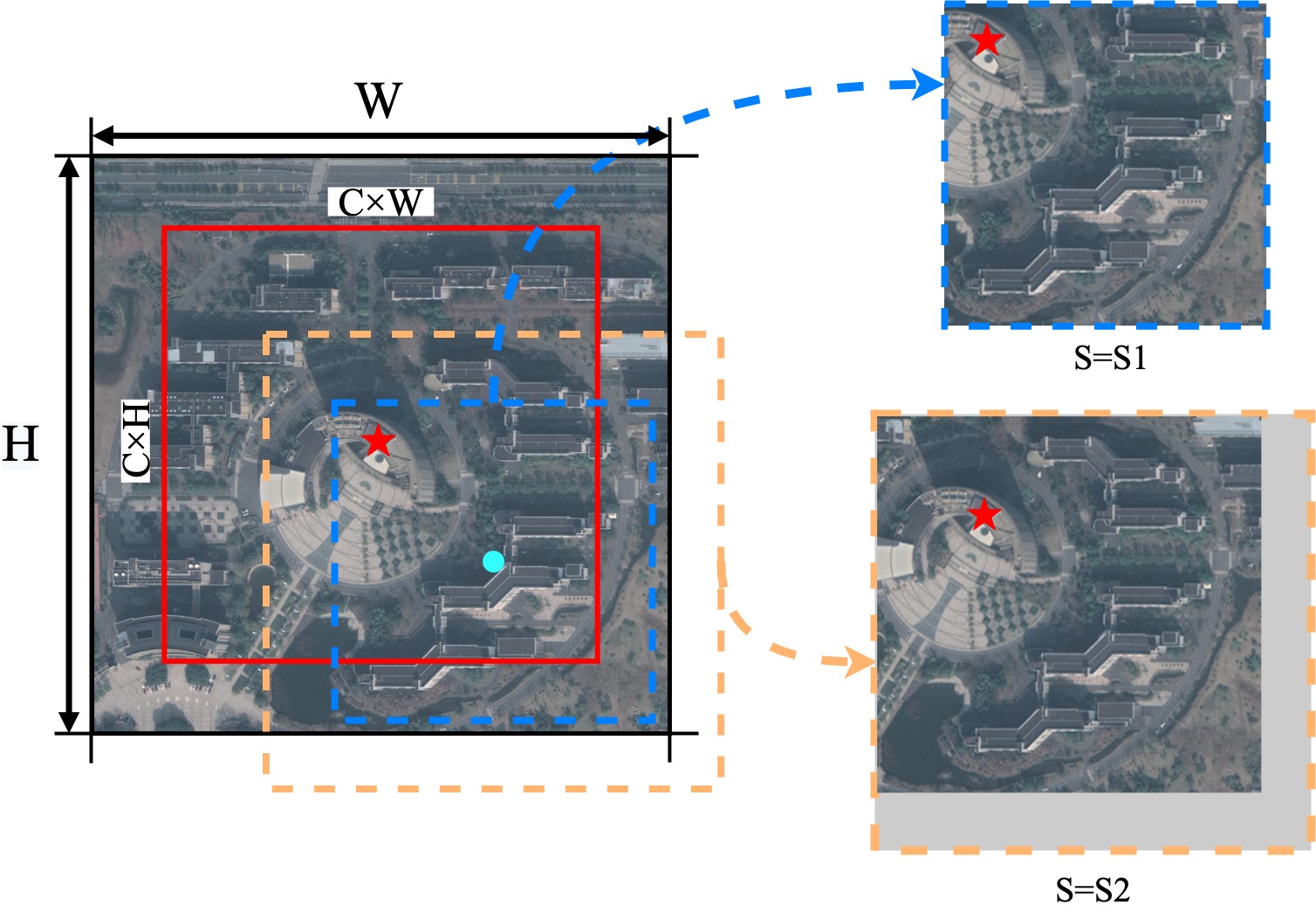
Figure 6: The process of the RSC augmentation method. The red pentagon is the position of the UAV. The light blue dot is the randomly generated center position of the image. The orange and blue dotted boxes correspond to 2 cropped images of different scales.

There are mainly two types of data construction schemes for FPI training. One is to pre-build UAV-satellite pairs. The other is to generate pairs randomly through data augmentation. We adopt the latter for better flexibility and design a random scale and offset augmentation method named Random Scale Crop (RSC). The proposed RSC can simultaneously generate sample pairs with random target distributions and random scales. Fig. 6 depicts the implementation of RSC, in which we create two hyperparameters to dynamically crop satellite-view images in the training phase: one is the centroid coverage range C (0.85 in default), and the other is the scale range S (512$\rightarrow$1000 in default). C determines the distribution interval of the query in the search map. The smaller C is, the closer the query is distributed in the middle of the search map. S determines the spatial scale of the search map. The larger the S is, the greater the spatial distance occupied by the unit pixel after resizing. The purpose of RSC is to improve the model’s ability to resist scale and offset. More simply, C determines the size of the red area where query can be distributed. By setting different S (S1 and S2), we generated search maps of different scales. However, there still have a mandatory requirement for setting the S, that is, the query must be included in the search map.

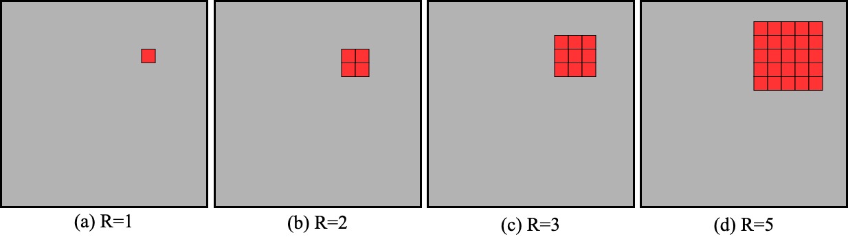
Figure 7: Schematic diagram of selecting positive samples according to R.

Algorithm 1 Weighted Balance Loss.

0:  $\textit{map}\in{\mathbb{R}^{\textit{H}\times\textit{W}}}$, $\textit{label}\in{\mathbb{R}^{\textit{H}\times\textit{W}}}$, $\textit{w}_{\textit{neg}}\in{\mathbb{R}}$, $\textit{R}\in{\mathbb{N}^{+}}$

0:  loss # Generate the 0,1 matrix as shown in Fig. 7

1:  $(\textit{map},\textit{label},R)\Rightarrow t$ # Num of the positive and negative samples

2:  $\textit{w}\leftarrow\textit{t}$

3:  $\textit{N}_{\textit{pos}}=\textit{R}^{2}$

4:  $\textit{N}_{\textit{neg}}=\textit{H}\times\textit{W}-\textit{R}^{2}$ # Weight of the positive and negative samples

5:  $\textit{W}_{\textit{pos}}=1/\textit{N}_{\textit{pos}}$

6:  $\textit{W}_{\textit{neg}}=(1/\textit{N}_{\textit{neg}})\times{\textit{w}_{\textit{neg}}}$ # Weight normalization

7:  $\textit{w}\leftarrow\textit{w}/\sum{\textit{w}_{\textit{i}}}$ # Map normalization

8:  $\textit{p}\leftarrow\textit{sigmoid}(\textit{map})$ # Weighted balance loss

9:  $\textit{loss}=-\sum({{\textit{log}(\textit{p}_{\textit{ij}})\textit{t}_{ij}\textit{w}_{\textit{ij}}}+{\textit{log}(1-\textit{p}_{\textit{ij}})(1-\textit{t}_{\textit{ij}})\textit{w}_{\textit{ij}}}})$

10:  return  loss

III-E Weighted Balance Loss (WBL)

The number of positive and negative samples, as well as their weights, are important variables in the process of model optimization. Samples imbalance will lead to learning an extreme mode to minimize the loss function, which may mislead the model or slow down its convergence speed. Balance Loss [30] is an effective method to balance positive and negative samples, with its core principle being to maintain a 1:1 weight between positive and negative samples. However, Balance Loss does not adequately handle the balance between the number of positive and negative samples, and a perfect 1:1 balance is not conducive to the convergence for the localization task. Therefore, an improved method called Weighted Balance Loss (WBL) is proposed to address the above issues whose pseudo-code is shown in Algorithm 1. WBL treats samples within a certain range R around the ground truth as positive samples and uses $\textit{w}_{\textit{neg}}$ to adjust the impact of negative samples.

In particular, R is chosen as the sampling cut-off to divide the positive and negative samples. As shown in Fig. 7, R=1 means that only the position closest to ground-truth is taken as positive, and the rest are all negative. R=2 means that the four points around ground-truth are taken as positive samples. By analogy, as R increases, the number of positive samples gradually increases, but the weight assigned to each positive sample will also decrease accordingly.

In terms of sample weights, firstly, the number of positive and negative samples should be counted. A weight matrix whose size is the same as the heatmap needs to be prepared to store the weight of each sample. Since the number of negative samples is much larger than that of positive, the weight of each positive is much larger than that of the negative after balancing. Therefore, $\textit{w}_{\textit{neg}}$ is introduced to dynamically adjust the weights for negative samples. Last, the weight matrix is multiplied by the cross-entropy loss value for all samples.

IV Dataset and Evaluation

TABLE I: Geo-localization dataset information summary.

Datasets	UL14 (ours)	DenseUAV[8]	SUES-200[16]	University-1652[15]	VIGOR[14]	CVUSA[12]
Training	6.8k$\times$2	10$\times$225.6$\times$9	120$\times$51	701$\times$71.64	91k+53k	35.5k$\times$2
Platform	Drone, Satellite	Drone, Satellite	Drone, Satellite	Drone, Ground, Satellite	Ground, Satellite	Ground, Satellite
Imgs./Platform	1 + 1	3 + 6	50 + 1	54 + 16.64 + 1	/	1 + 1
Target	UAV	UAV	Diverse	Building	User	User
Method	FPI	IR	IR	IR	IR + Reg	IR
Evaluation	RDS & MA	R@K & SDM	R@K & AP & RB & PF	R@K & AP	MA	R@K

TABLE II: Statistical table for the UL14 dataset. Where #University refers to the number of universities included.

#Subset	#Imgs		#Universities
	UAV-view	Satellite-view
Train	6768	6768	10
Test	2331	27972	4

IV-A Dataset Description

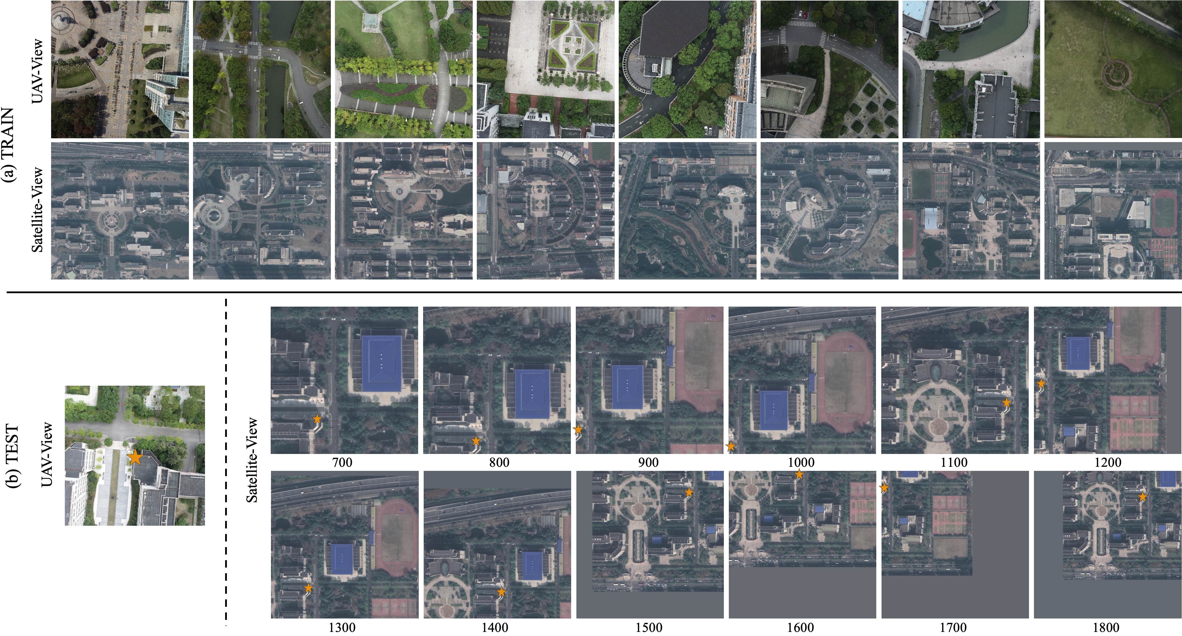
Figure 8: Visualization of some samples in the train and test set. The numbers in the test set represent the original pixel scale (0.294 meters/pixel).

We adopted the UAV-view images from DenseUAV and collected the corresponding 20-level satellite-view images from Google Maps to construct the UL14 dataset. Table I lists the amount of training data, sampling platforms, data distribution, localization targets, and evaluation metrics for some typical geo-localization datasets. Explicitly, the UL14 dataset possesses the following characteristics. 1) Image from two perspectives: UAV and satellite views. 2) Paired training data: the UAV images and satellite images in the training data are constructed in pairs, and the data augmentation method will be used in the actual training process to expand the diversity of paired data. 3) Multiple flight altitudes: UAV images are sampled in three flight altitudes (80, 90, and 100 meters). 4) Multi-scale test data: The test satellite data is constructed of 12 different scales to enhance the difficulty of positioning.

Next, we will provide a detailed introduction to the construction of the train and test set, and the quantity statistics are presented in Table II.

IV-A1 Train Set

The training set comprises images collected by 10 universities. The UAV-view images are captured from three different flight heights: 80, 90, and 100 meters. Conversely, the satellite-view images are obtained using 20-level Google Maps satellite imagery. To enhance the utility of the training set, the resolution of UAV-view images is uniformly set to (512, 512), while the satellite images are set to (1280, 1280). The decision to retain larger satellite images is made to allow for greater flexibility in subsequent data augmentation, which will be discussed in Section III-D. Last, some paired images of the train set are shown in Fig. 8(a).

IV-A2 Test Set

The test set comprises images collected by 4 universities, with no overlap with the train set. The spatial scale of the satellite images is defined by setting the pixels in the range of 700-1800 (0.294 meter/pixel) at intervals of 100 pixels. This implies that each UAV image in the test set generated 12 satellite images of varying scales. Also, the position of the UAV in the satellite imagery is randomly distributed, either in the center or at the edge. For a clear view, one set of images in the test set is shown in Fig. 8(b).

IV-B Evaluation Indicators

Recall@K and AP[50, 51] are commonly used evaluation metrics, which only consider whether the sample is positive or negative. This is a kind of discrete metric, which defeats the real purpose of the localization task. Unlike the indirect positioning of the image retrieval scheme, FPI needs a more intuitive way to evaluate the accuracy of localization. Therefore, we propose two evaluation metrics, Meter-level Accuracy (MA) and Relative Distance Score (RDS), to evaluate the localization accuracy from the space- and model-level respectively.

IV-B1 Meter-level Accuracy (MA)

One intuitive way to measure localization accuracy is to analyze it from the level of spatial distance, that is, to measure the Meter-level Accuracy (MA). The expression of the MA evaluation index proposed in this paper is as follows:

$$\text{MA@K}=\frac{\sum_{i=1}^{N}{1_{\text{SD}<\text{Km}}}}{N}$$ (1)

$$1_{\text{SD}<\text{Km}}=\begin{cases}1&\text{SD}<\text{Km}\\ 0&\text{SD}\geq\text{Km}\end{cases}$$ (2)

where SD refers to the real spatial distance in meters. K is an adjustable parameter. MA@K refers to the number of samples with positioning errors within Km as a proportion of the total samples. In conclusion, MA@K can be represented as the accuracy of positioning error less than Km. The expression of SD is as follows:

$$\text{SD}=\sqrt{(\Delta{x})^{2}+({\Delta{y}})^{2}}$$ (3)

$\Delta{x}$ denotes the meter-level error between the model prediction and the ground-truth in the longitude direction, and $\Delta{y}$ denotes the meter-level error in the latitude direction.

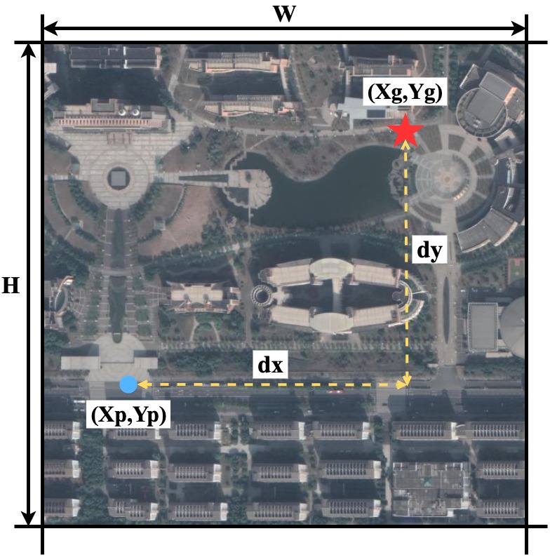
Figure 9: Schematic diagram of the RDS, with the pentagram indicating ground-truth and the blue circle indicating the position predicted by the model.

IV-B2 Relative Distance Score (RDS)

Although MA can express the accuracy of positioning intuitively, it also has some shortcomings. 1) The setting of K has different effects on search maps of different scales. For large-scale search maps, after resizing, the spatial distance represented by a unit pixel will also become larger. Therefore, there will be a small deviation in the search map, but a large deviation in the spatial distance. 2) MA often needs to be expressed by a series of K, which is not convenient for directly expressing the performance of the model.

Based on the above discussion, we propose the Relative Distance Score (RDS) to evaluate from the model level. As shown in Fig. 9, $(X_{p},Y_{p})$ represents the predicted coordinates and $(X_{g},Y_{g})$ represents the ground-truth coordinates. The expression for Relative Distance (RD) is as follows:

$$\text{RD}=\sqrt{\frac{(\frac{dx}{w})^{2}+(\frac{dy}{h})^{2}}{2}}$$ (4)

where $dx=\left|X_{p}-X_{g}\right|$ and $dy=\left|Y_{p}-Y_{g}\right|$. To make the RD perform in the same direction as the accuracy and distributed between 0 and 1. We convert the distance into a score, and the expression of the converted RDS is as follows:

$$\text{RDS}=e^{-k\times\sqrt{\frac{(\frac{dx}{w})^{2}+(\frac{dy}{h})^{2}}{2}}}$$ (5)

where $k$ is the scaling factor, which is set to 10 by default.

Why propose an RDS? First of all, RDS measures the performance of the model by the relative distance at the pixel level in the image, which can resist the scale transformation of the search map. The distance in RDS is no longer the real space distance, but the pixel distance in the image, which is beneficial to evaluate the performance from the model level. Second, the RDS is an overall score, which is distributed between 0 and 1, and is positively correlated with the positioning accuracy, that is, the higher the RDS, the higher the positioning accuracy. Finally, RDS uses an exponential method to expand the relative distance. When the distance increases, the RDS will return to 0 in an exponential form, which is in line with the expectation that the large distance deviation will be regarded as a wrong positioning.

V Experiment

V-A Implementation Details

In the experiments, all initial parameters of backbones are pre-trained on ImageNet[52]. The AdamW[53] optimizer is adopted with a weight decay of 5e-4. Moreover, we incorporate a cosine annealing learning rate decay schedule, and the minimum learning rate is 1/100 of the initial learning rate. Furthermore, To compare under the same conditions, FPI-series models are trained for 12 epochs, with batch size setting to 8. For the inference phase, the hanning window size is the same as the training setting of R in WBL. Mixed-precision training strategy is applied in all models.

V-B FPI v.s. Image Retrieval

V-B1 Localization Performance

TABLE III: Compare the performance of the FPI and image retrieval.

Type	Method	TTA	MA@3	MA@10	MA@20
Image Retrieval	Uni-1652(ViT-S)	MS+MT	0.099	0.607	0.836
	LPN(ViT-S)[28]	MS+MT	0.116	0.613	0.806
	FSRA-2B[29]	SS	0.079	0.580	0.743
	FSRA-2B[29]	MS	0.090	0.586	0.755
	FSRA-2B[29]	MS+MT	0.126	0.650	0.832
FPI	FPI-PF(ours)	/	0.084	0.436	0.643
	FPI-MF(ours)	/	0.131	0.625	0.837

Due to the inconsistent evaluation methods of FPI and image retrieval. We additionally added the MA@K evaluation metric for DenseUAV. Since the test set of DenseUAV is constructed at intervals of 20m and the gallery contains images that perfectly match each query, we have additionally constructed a gallery of satellite images with a sampling interval of 10m and not perfectly center-corresponding. The experimental results are shown in Table III. We have used three previous SOTA models in image retrieval for comparative experiments. Several conclusions can be drawn as follows: (1) The end-to-end architecture (FPI) can achieve positioning performance similar to or even better than image retrieval. The FPI-MF surpasses image retrieval methods with TTA on MA@3 and MA@20. (2) Test Time Augment (TTA) can effectively improve the positioning effect of image retrieval. (3) TTA will directly increase storage and computing consumption. If TTA is not used, FPI is far stronger than image retrieval in localization accuracy.

V-B2 Efficiency

The detailed time consumptions of FPI and image retrieval are counted in Table IV, which contains 600 samples. The main steps are as follows:

• Building Satellite Gallery (BSG): Intensive split of satellite images to construct a gallery database just like the process in Fig. 1(a). For image retrieval, the split pre-process will cost 4.2s for SS and 17.6s for MS+MT. For FPI, It is only necessary to crop the corresponding image from the satellite image in memory which costs 0.1s or even less time.

• Gallery Forward Propagation (GFP): Extract features for all images in the gallery. For image retrieval, time consumption depends on the number of images in the gallery. For FPI, no additional time consumption is required.

• Inference And Localization (IAL): Real-time inference and localization. For image retrieval, It is necessary to calculate the cosine similarity between the UAV and satellite features, and calculations depend on gallery scale and saved feature dimension. For FPI, only model inference is needed, which costs 6s for FPI-MF structure much faster than the 100.2s of image retrieval.

The above data is obtained without considering optimization. Of course, the image retrieval method can be optimized with parallel algorithms in the pre-processing and feature extraction parts, and GPU can also be used for acceleration in post-processing. But from the perspective of overall efficiency, FPI still has an absolute advantage.

TABLE IV: Time consumption comparison of FPI and image retrieval.

Method	TTA	BSG	GFP	IAL	Total
FSRA-2B	SS	4.2s	6.5s	43.2s	53.9s
FSRA-2B	MS	9.1s	15.2s	77.4s	101.7s
FSRA-2B	MS+MT	17.6s	25.9s	100.2s	143.7s
FPI-SF	/	0.1s	0s	6.2s	6.3s
FPI-MF	/	0.1s	0s	6s	6.1s

V-B3 Storage Consumption

Next, the FPI and image retrieval schemes will be compared from the perspective of disk storage. The results are shown in Table V. The main consumption is as follows:

• Gallery Images (GI): For image retrieval, it is necessary to densely slice the satellite image and store them on disk (44.6MB for SS and 266MB for MS+MT). For FPI, only a big satellite image is required (4.8MB).

• Gallery Features (GF): For image retrieval, the gallery needs to perform forward propagation to obtain the satellite features (10.8MB for SS and 60.6MB for MS+MT). For FPI, no additional storage consumption is required.

To sum up, FPI consumes only 4.8MB during the localization process of 600 samples, which is nearly 1/68 of the image retrieval scheme (326.6MB). If temporarily stored image data is not considered here, FPI is still an order of magnitude behind image retrieval (4.8MB v.s. 60.6MB). Therefore, FPI also has an absolute advantage in disk storage consumption.

TABLE V: Storage consumption comparison of FPI and image retrieval.

Method	TTA	GI	GF	Total
FSRA-2B	SS	44.6MB	10.8MB	55.4MB
FSRA-2B	MS	133.2MB	33.1MB	166.3MB
FSRA-2B	MS+MT	266MB	60.6MB	326.6MB
FPI-SF	/	4.8MB	0MB	4.8MB
FPI-MF	/	4.8MB	0MB	4.8MB

V-C Impact of Satellite Spatial Scale

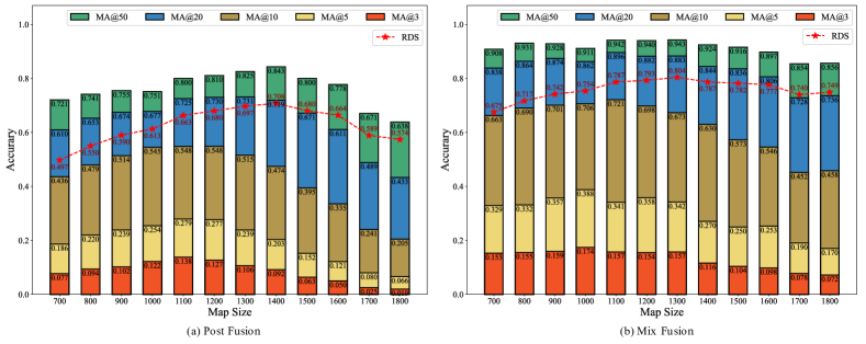
Figure 10: The impact of search mapsize on the positioning of two FPI structures, including RDS and MA@K indicators.

The spatial scale of the search map directly determines the fine-grained information of the input satellite image. Given that the scale of the model input is typically fixed, the model’s resistance to scale shifts is important. To investigate the influence of different scales of search maps, we conducted a series of comparison experiments with satellite images ranging from 700 to 1800 pixels (0.294 meters/pixel).

On the one hand, the results of the Post Fusion structure are presented in Fig. 10(a). We can observe a marked decline in the MA@K index as the scale of the satellite images increases, particularly evident in higher precision indicators like MA@3, MA@5, and MA@10. This trend can be easily rationalized. Given that the input size for all models is consistent, larger satellite image scales would mean that each pixel in the input image represents a larger actual spatial distance. For instance, when the mapsize is 700, the corresponding actual spatial distance is 205.9m. If the output feature map size from the model is 384, then the actual spatial distance between each pixel in the feature map is 0.536m. However, when the mapsize is 1800, it becomes 1.206m. Although larger mapsize yield poorer localization performance, it is still necessary to use them. The reason lies in the fact that large mapsize can simplify the actual process of UAV self-localization. For instance, if one large image can resolve the localization of all positions, it eliminates the need for any post-processing operations on the application side. Further observing the change rule of RDS, we can find that the overall curve is relatively smooth, but it is worth noting that it does not perform well at small scales. This is mainly due to the fact that small-scale images cover less spatial information and the loss of edge information is exacerbated.

On the other hand. the results of the Mix Fusion structure are shown in Fig. 10(b). It is evident that, compared to the Post Fusion structure, Mix Fusion exhibits better robustness to scale. Although it also follows the aforementioned trend, but smoother. This is primarily because deeper information interaction and fusion can assist the model in better learning spatial distribution information.

V-D Impact of Query Distribution

Figure 11: (a) Query distributions. (b) MA curves under different spatial distributions. (c) RDS and sample number under different spatial distributions.

During the application, the relative position of the query in the search map is uncertain due to factors such as time delays and flight speed. Therefore, it is important to explore the impact of query distribution. As shown in Fig. 11(a), we divide different ranges according to the relative spatial distance between the query and the center point of the search map. The MA curve is shown in Fig. 11(b). We can clearly see that there is a significant decrease in localization accuracy when queries are located in the region >1.0. This is consistent with our expectations, to take an extreme example, when the query is located on 4 corners of the search map, only 1/4 of the information will be available, and the remaining 3/4 of the image information will not find the corresponding information on the search map, which undoubtedly increases the challenge of localization. Furthermore, Fig. 11(c) illustrates the number of samples, as well as the RDS for each region. The quantity distribution is approximately proportional to the area of the region, which results in fewer samples in the 0-0.2 range and more in the 0.8-1.0 range. From the RDS, we can similarly observe a cliff-like decline in the results for the >1.0 region. This decline is attributable to the loss of edge information, which greatly affects the discriminative ability of the model. In conclusion, queries located on the edge of the search map significantly reduce localization accuracy.

V-E Impact of Flight Altitude

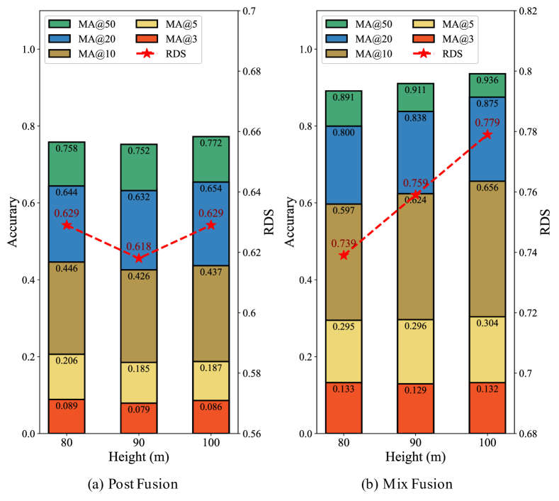
Figure 12: MA@K and RDS of UAV at different flight altitudes.

In the application scenario, the altitude of the UAV flight is an uncertain factor, which directly affects the spatial scale of the query. Taking this into account, UL14 collected UAV images from 80, 90, and 100m altitudes. In the testing phase, data of different heights are divided for separate testing. The experimental results of the two architecture models are shown in Fig. 12. It can be seen that both MA@K and RDS show relatively stable performance at these three different heights. However, due to factors such as the height limit of the UAV, higher data have not been collected to fully verify the robustness of the model to flight heights.

VI Model Analysis

VI-A Model Stucture

TABLE VI: Table of experimental results for two model architectures.

Structure	Fusion Method	Macs	Params	InferTime	RDS	MA@3	MA@5	MA@10	MA@20	MA@50
Post Fusion	GC	13.3G	39.3M	24.0s	0.576	0.043	0.111	0.329	0.581	0.727
	SAF	13.5G	39.6M	27.5s	0.293	0.001	0.004	0.026	0.091	0.374
	CAF	13.4G	39.5M	27.0s	0.287	0.001	0.003	0.025	0.086	0.358
Mix Fusion	Mix+AvgPool	13.1G	19.6M	22.4s	0.680	0.043	0.132	0.418	0.725	0.875
	Mix+Linear	13.2G	19.7M	21.3s	0.681	0.045	0.137	0.430	0.721	0.873
	Mix+GeM	13.1G	19.7M	21.6s	0.680	0.042	0.134	0.423	0.727	0.871
	Mix+GC	13.2G	19.6M	21.5s	0.670	0.056	0.146	0.427	0.711	0.850

VI-A1 Post Fusion (FPI-PF)

We conducted experiments on the three fusion methods, GC, SAF, and CAF, as shown in Table VI. In terms of computation and parameter quantities, the computation of SAF is 0.2GMacs higher than that of GC, and its parameter quantity is 0.3M larger than that of GC, with CAF being slightly lower than SAF. Regarding inference speed, SAF is significantly slower than GC and slightly slower than CAF. However, in terms of model accuracy, the fusion method of GC significantly outperforms the CAF and SAF methods across all indicators. This is a perplexing phenomenon. In the field of SOT, the fusion methods based on attention can interact more fully with features and help alleviate scale inconsistency issues. We attribute this phenomenon to the data level. Given that the input data is from different sources and that there are challenges like rotation uncertainty and spatial information inconsistency due to time, which increases the complexity of learning relationships between features. For attention methods, it means that more training data and iterations are required to learn general knowledge. Conversely, the GC-based method interacts with features using a sliding window, which restricts the spatial scale and makes it easier for the model to learn certain patterns.

VI-A2 Mix Fusion (FPI-MF)

Unlike Post Fusion, Mix Fusion can be regarded as a single-stream structure that adds an attention module for feature fusion in blocks of the backbone. As shown in Table VI, compared to the Post Fusion, Mix Fusion possesses significant advantages in terms of parameters, speed, and localization accuracy. Specifically, RDS improved from 0.576 to 0.681, a boost of 10.5 points, and MA@20 increased by 14.6%. This is primarily due to Mix Fusion enabling deep interaction of context information from the two domains and effectively overcoming the scale inconsistency problem introduced by the GC-based method. Furthermore, within the framework of Mix Fusion, we adopted four different methods to compress the number of channels for training: AvgPool, Linear, GeM[54], and GC. As a result, the Linear method achieved the best result on RDS, reaching 0.681, and reached the fastest inference speed of 21.3s/1000samples. It is worth mentioning that the GC method effectively improves the short-distance positioning accuracy, which is the advantage of introducing additional prior inductive bias.

VI-B RSC Data Augmentation

In the experiments, three scale augmentation schemes, namely single scale, multiple scale, and random scale are implemented. As shown in Table VII, [512, 768] denotes scales of 512 and 768, meanwhile, 512$\rightarrow$768 indicates the random integers down to 512 and up to 768. It can be observed that models trained using single scale underperform in localization tasks. In contrast, both multiple scale and random scale methods result in substantial improvements. This observation aligns with our expectations, as having the model learn universal rules of localization across different scales during training can enhance the model’s robustness to scale during testing. Ultimately, our baseline model employs the random scale (512$\rightarrow$1000) augmentation scheme.

TABLE VII: The results of different scale strategies

Scale Type	Scale	RDS	MA@5	MA@20
Single Scale	512	0.529	0.109	0.524
	768	0.533	0.081	0.489
	1000	0.395	0.024	0.238
Multiple Scale	[512, 768]	0.607	0.127	0.628
	[768, 1000]	0.639	0.112	0.648
	[512, 768, 1000]	0.671	0.146	0.703
Random Scale	512$\rightarrow$768	0.606	0.126	0.631
	768$\rightarrow$1000	0.592	0.087	0.574
	512$\rightarrow$1000	0.680	0.137	0.721

VI-C Feature Scales

TABLE VIII: The impact of different feature scales and feature fusion methods. $\rightarrow$ represents an up-sampling operation.

Multi-Scale Structure	Output Scale	RDS	MA@3	MA@5	MA@10	MA@20	MA@50	MA@100
Baseline	(H/16, W/16)	0.680	0.045	0.137	0.430	0.721	0.873	0.939
Upsample	(H/8, W/8)	0.717	0.089	0.220	0.518	0.773	0.893	0.948
	(H/4, W/4)	0.731	0.100	0.244	0.557	0.795	0.899	0.949
	(H/2, W/2)	0.728	0.105	0.243	0.547	0.788	0.897	0.948
	(H/1, W/1)	0.730	0.109	0.251	0.561	0.790	0.893	0.946
Feature Pyramid	(H/8, W/8)	0.733	0.114	0.270	0.584	0.796	0.844	0.940
	(H/4, W/4)	0.732	0.117	0.267	0.573	0.802	0.888	0.936
	(H/4, W/4) $\rightarrow$ (H/2, W/2)	0.753	0.126	0.287	0.614	0.832	0.908	0.949
	(H/4, W/4) $\rightarrow$ (H/1, W/1)	0.758	0.131	0.298	0.625	0.837	0.912	0.953

VI-C1 Multi-Scale Stucture

Experiments for two multi-scale schemes are formulated as shown in Table VIII. Overall, it can be seen that the feature pyramid has achieved noticeable improvements over the brutal upsampling operation. For instance, the RDS of feature pyramid on the (H/1, W/1) scale has increased from 0.730 to 0.758, which is a nearly 2.8 points rise, and an increase of 6.4% on MA@10. Similarly, there are noticeable improvements on other scales as well. As we know, deep features always contain high-level semantic information, while shallow features carry information such as outline and color. The fusion of shallow features can provide more information for discrimination. However, the significant improvement also demonstrates the necessity of pyramid features in this task.

VI-C2 Output Resolution

The feature resolution of the final layer based on the CvT13 (Baseline in Table VIII) is 1/16 of the original image. In the experimental process, we enlarged the feature scale by a factor of 2 until it matched the original input. However, for the feature pyramid structure, to restore the original scale, we additionally employed bilinear interpolation for up-sampling. As shown in Table VIII, it is evident that with the increase of the output scale, most of the metrics show an upward trend, particularly on the small distance error metrics such as MA@3 and MA@5, which is expected. Due to the enlargement of the output scale, the real spatial distance corresponding to a unit pixel in the output heatmap will become smaller. Therefore, the actual distance deviation caused by wrongly predicting one pixel is multiplicatively reduced. This experiment also verifies a hypothesis that the output scale of the model significantly affects the performance.

VI-D Backbones

TABLE IX: Table of experimental results for different backbone networks.

Type	Structure	Backbone	Macs	Params	InferTime	RDS	MA@3	MA@5	MA@10	MA@20
CNN	Hierarchical	ResNet50[55]	13.7G	47.2M	9.9s	0.208	0.001	0.004	0.016	0.059
		EfficientNet-B5[56]	7.44G	54.3M	33.1s	0.402	0.007	0.020	0.078	0.273
		ConvNext-T[57]	14.6G	55.7M	8.1s	0.465	0.022	0.058	0.198	0.412
Transformer	Unstructured	ViT-S[40]	13.9G	43.3M	9.9s	0.577	0.038	0.099	0.313	0.564
		ViT-B[40]	55.0G	171.5M	10.3s	0.595	0.050	0.126	0.363	0.597
		DeiT-S[41]	13.9G	43.3M	9.7s	0.597	0.048	0.123	0.358	0.604
	Hierarchical	PvT-S[42]	12.0G	47.3M	18.3s	0.524	0.020	0.054	0.169	0.470
		CvT13[43]	13.3G	39.3M	25.2s	0.576	0.043	0.111	0.329	0.581

Existing mainstream backbone networks can be divided into CNN-based and Transformer-based. In experiments, ResNet50, EfficientNet-B5, and ConvNext-T are adopted in the CNN-based category. Also, Transformer-based models are divided into two types: Unstructured and Hierarchical. The Unstructured denotes the type of native ViT architecture including ViT-S, ViT-B, DeiT-S, whereas Hierarchical refers to models possessing hierarchical architecture such as PvT-S and CvT13. To ensure fairness, all weights of backbones are pretrained from the timm [58] framework, and the FPI-PF structure with GC is adopted.

The experimental results are shown in Table IX. Some conclusions are summarized as follows. Firstly, the Transformer-based backbone significantly outperforms the CNN-based ones. This is primarily because the UAV self-localization task is characterized by numerous challenges such as domain difference, rotation uncertainty, viewpoint offset, and time-induced spatial information differences. Hence, this task demands networks with the capability to globally model and excavate contextual semantic information, which is the strength of the Transformer. Secondly, Unstructured Transformer models can achieve relatively good performance, which is mainly due to the fact that shallow features are not fully utilized here. Yet, among the Hierarchical queue, the CvT13 backbone network not only possesses the characteristic of hierarchical feature output but also achieves relatively good performance. In the end, we chose CvT13 as the backbone network of our baseline because it has the characteristics of a hierarchical network, which will facilitate multi-scale feature fusion and show excellent performance.

VI-E Loss Functions

VI-E1 Loss Type

In the experiments, we trained with four different loss functions: cross-entropy loss, focal loss, balance loss, and the proposed weighted balance loss (WBL). The experimental results are shown in Table X. The performance of using balance loss alone is far worse than using cross-entropy loss or focal loss. As a result, a complete balance of positive and negative samples is not conducive to model convergence. Since the number of positive samples is much smaller than that of negative samples, the weight assigned to a single negative sample will be much smaller than that of positive samples after balancing. However, the results based on WBL lead to a 10-points RDS increase, and all MA@K indicators also achieve significant improvements.

TABLE X: Table of experimental results for different loss functions.

Loss	RDS	MA@5	MA@10	MA@20
Focal Loss[59]	0.730	0.261	0.578	0.794
CrossEntropy Loss[60]	0.750	0.276	0.606	0.828
Balance Loss[61]	0.654	0.197	0.455	0.676
Weighted Balance Loss	0.758	0.298	0.625	0.837

VI-E2 Negative Weight

To find the most suitable value of $\textit{w}_{\textit{neg}}$, we made a lot of experiments with $\textit{w}_{\textit{neg}}$ as the variable, and the experimental results are shown in the table XI. When $\textit{w}_{\textit{neg}}=1$, the proposed WBL is equivalent to Balance Loss. When $\textit{w}_{\textit{neg}}$ reaches 130, all indicators are reaching the optimal state, as $\textit{w}_{\textit{neg}}$ keeps increasing, and all indexes gradually decrease. Last, $\textit{w}_{\textit{neg}}=130$ is adopted in our baseline.

TABLE XI: Table of experimental results for different negative weights.

Negative Weight	RDS	MA@5	MA@10	MA@20
1	0.654	0.197	0.455	0.676
10	0.728	0.271	0.570	0.787
30	0.722	0.274	0.571	0.779
50	0.748	0.276	0.600	0.820
80	0.744	0.279	0.603	0.819
100	0.739	0.270	0.588	0.810
110	0.749	0.284	0.606	0.825
120	0.753	0.295	0.621	0.834
130	0.758	0.298	0.625	0.837
140	0.742	0.276	0.593	0.819
150	0.743	0.276	0.593	0.819
160	0.740	0.265	0.591	0.816
200	0.737	0.251	0.581	0.815

VI-F Input Scale

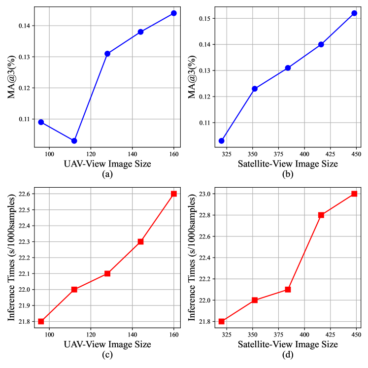
Figure 13: The impact of varied input scales on the performance of localization.

High-resolution input can provide more fine-grained information. We conduct two sets of comparison experiments on input images. One group is to control the UAV image scale as 128 pixels and change the satellite image scale (320$\rightarrow$448 pixels; stride=32), The other group is to control the satellite image scale as 384 pixels and change the UAV image scale (96$\rightarrow$160 pixels; stride=16). The results are shown in 13(a)(b), we can conclude that as the input scale increases, the positioning performance generally shows a positive correlation trend. Additionally, the inference time is counted in Fig. 13(c)(d). It can be seen that the effect of the image scale variation of UAV on the inference time is smaller, mainly because the image scale of UAV is much smaller compared to satellite. Last, the resolutions of satellite and UAV images used for our baseline are 384 and 128 pixels, respectively.

VI-G Sharing Weight in FPI-PF

TABLE XII: Experimental results table of the influence of padding and weight sharing on the localization effect.

Structure	Padding	Sharing	RDS	MA@5	MA@20
Post Fusion	$\times$	$\times$	0.407	0.016	0.226
	✓	$\times$	0.576	0.111	0.581
	✓	✓	0.276	0.003	0.093
Mix Fusion	$\times$	$\times$	0.571	0.049	0.493
	✓	$\times$	0.680	0.137	0.721

Weight sharing can help reduce the parameters. As shown in Table XII. We find that the training process converges very slowly and performance is extremely poor when weights are shared. That is because the two-source data inputs have a massive domain difference, with uncertainties like viewpoint bias and rotation. Additionally, unlike CVGL tasks, this task needs to fuse features and learn the spatial consistency relationship between two domains. Non-sharing allows for more differences in the learning process of the two domains.

VI-H Padding in GC

Both structures of Post-Fusion and Mix-Fusion can use GC for feature fusion in their output stages. However, we find that padding in GC plays a crucial role in maintaining spatial position information. The padding setting is to make the kernel center slide over each pixel of the source, ensuring that the spatial information of the output feature map is consistent with the original source. As shown in Table XII, the introduction of padding in GC has resulted in significant improvements (16.9-points boost in RDS for Post-Fusion and 10.9-points boost in RDS for Mix-Fusion).

VII Visualization

According to the characteristics of the output feature map supervision, the heat map shows the spatial distribution of response strength after completing the sigmoid. That is, the higher the value in the heat map, the greater the probability. Based on this setting, we normalize the output feature map and directly visualize it to analyze the response results. The visualization results are shown in Fig. 14, which can be divided into 3 types of cases. From groups 1 and 2, it can be clearly observed that the structure based on Mix-Fusion presents more positive results in thermal response, without ambiguous thermal distribution. We believe that this is mainly due to the deep feature interaction method of Mix-Fusion, which allows the model to better understand spatial semantic information and thus generate more confident results. From groups 3 and 4, it can be seen that the FPI-MF structure is better at small distance deviations because Mix-Fusion allows the backbone to learn relative spatial distribution information in shallow features, thereby more precise positioning. Last, groups 5 and 6 are cases where FPI-MF performed poorly. However, when we compared the original input UAV images, there was indeed a great deal of similarity in the locations of the mismatches. For such scenes with very similar images in space, it is indeed a huge challenge for the model to have stronger fine-grained mining and spatial information identification capabilities.

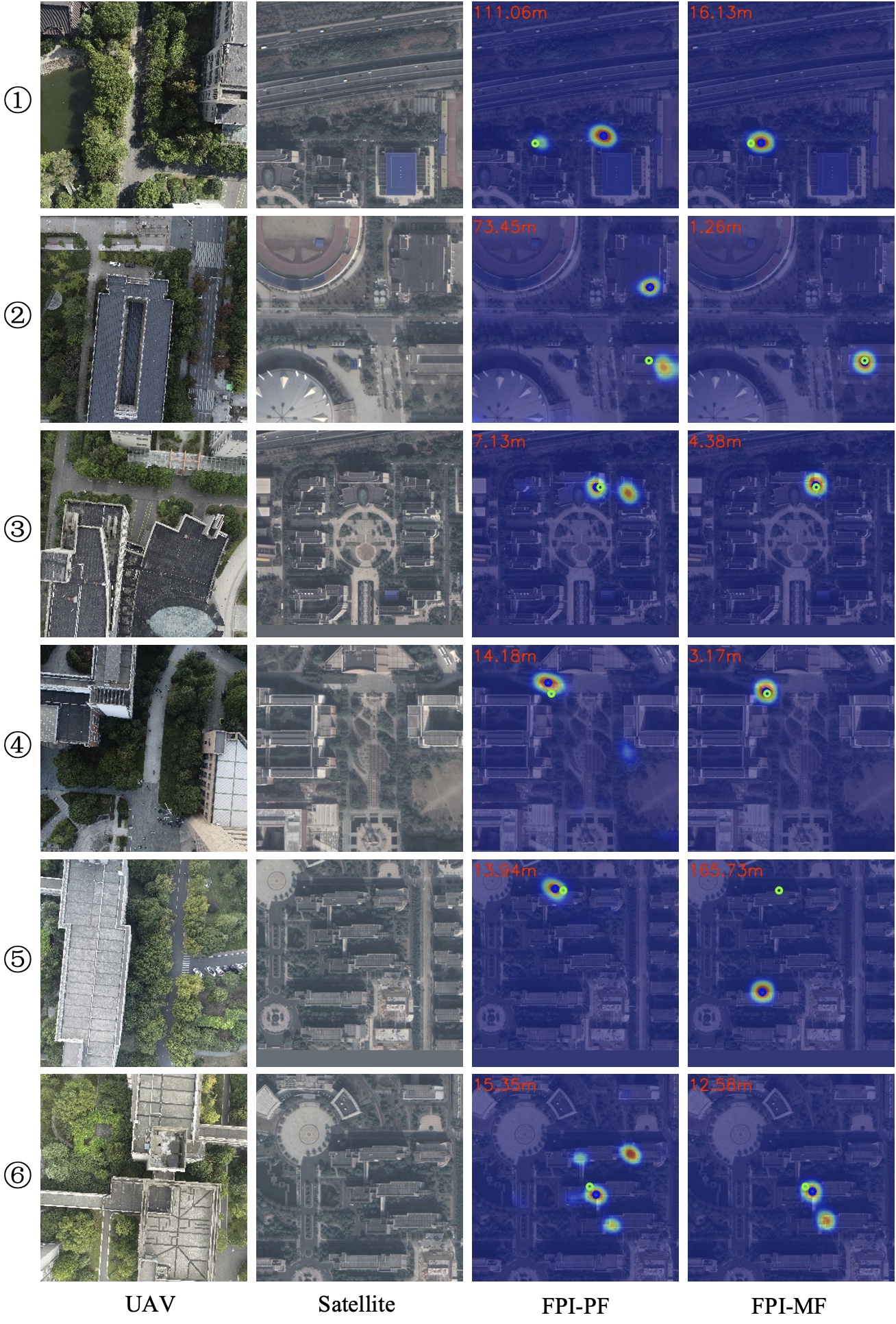
Figure 14: Visualization result graph of FPI. The first and second columns are the UAV and satellite images, and the third and fourth columns are the heatmaps of the FPI-PF and FPI-MF, respectively. The green circle is groundtruth, and the blue is the predicted position. The red number in the upper left corner is the positioning error, and the unit is meter.

VIII Conclusion

This paper introduces a simple and efficient end-to-end UAV self-localization architecture called Finding Point with Image (FPI), which simplifies the entire pipeline by eliminating complex pre-processing and post-processing present in image retrieval. Building upon the FPI, two model structures named Post Fusion (FPI-PF) and Mix Fusion (FPI-MF) are proposed, which are implemented as dual-stream and single-stream networks, respectively. To train the FPI model, a paired dataset (UL14) containing UAV and satellite images is constructed. Additionally, two evaluation metrics are presented to assess positioning accuracy: Meter-level Accuracy (MA) and Relative Distance Score (RDS). Furthermore, Random Scale Crop (RSC) augmentation method is proposed to expand paired data with random scales and offsets. Also, Weighted Balanced Loss (WBL) is proposed to emphasize the influence of negative samples in the training process. In addition, this paper carries out a large number of experimental analyses from the data and model levels to provide certain references for readers. For the two structures proposed in this paper, we have verified through experiments that the FPI-MF structure can achieve better positioning accuracy than the FPI-PF method. Finally, the proposed FPI-MF achieves comparable or even superior performance compared to the state-of-the-art image retrieval method, while significantly reducing inference time (1/24) and storage consumption (1/68).

References

- [1] Y. Zhu, B. Sun, X. Lu, and S. Jia, “Geographic semantic network for cross-view image geo-localization,” TGRS, vol. 60, pp. 1–15, 2022.
- [2] D. Turner, A. Lucieer, and L. Wallace, “Direct georeferencing of ultrahigh-resolution uav imagery,” TGRS, vol. 52, no. 5, pp. 2738–2745, 2014.
- [3] S. K. Roy, A. Deria, D. Hong, B. Rasti, A. Plaza, and J. Chanussot, “Multimodal fusion transformer for remote sensing image classification,” TGRS, vol. 61, pp. 1–20, 2023.
- [4] D. G. Lowe, “Distinctive image features from scale-invariant keypoints,” IJCV, 2004.
- [5] H. Bay, A. Ess, T. Tuytelaars, and L. V. Gool, “Speeded-up robust features (surf),” CVIU, 2008.
- [6] R. Mur-Artal, J. M. M. Montiel, and J. D. Tardós, “Orb-slam: A versatile and accurate monocular slam system,” TRO, vol. 31, no. 5, pp. 1147–1163, 2015.
- [7] M. Brown and D. G. Lowe, “Automatic panoramic image stitching using invariant features,” in IJCV, vol. 74, no. 1, 2007, pp. 59–73.
- [8] M. Dai, J. Zhuang, and E. Zheng, “Vision-based uav localization system in denial environments,” arXiv, 2022.
- [9] T.-Y. Lin, Y. Cui, S. Belongie, and J. Hays, “Learning deep representations for ground-to-aerial geolocalization,” in CVPR, 2015.
- [10] Y. Tian, C. Chen, and M. Shah, “Cross-view image matching for geo-localization in urban environments,” in CVPR, 2017.
- [11] N. N. Vo and J. Hays, “Localizing and orienting street views using overhead imagery,” in ECCV, 2016, pp. 494–509.
- [12] M. Zhai, Z. Bessinger, S. Workman, and N. Jacobs, “Predicting ground-level scene layout from aerial imagery,” in CVPR, 2017.
- [13] L. Liu and H. Li, “Lending orientation to neural networks for cross-view geo-localization,” in CVPR, 2019.
- [14] S. Zhu, T. Yang, and C. Chen, “VIGOR: Cross-view image geo-localization beyond one-to-one retrieval,” in CVPR, 2021.
- [15] Z. Zheng, Y. Wei, and Y. Yang, “University-1652: A multi-view multi-source benchmark for drone-based geo-localization,” in ACMMM, 2020, pp. 1395–1403.
- [16] R. Zhu, L. Yin, M. Yang, F. Wu, Y. Yang, and W. Hu, “Sues-200: A multi-height multi-scene cross-view image benchmark across drone and satellite,” TCSVT, pp. 1–1, 2023.
- [17] F. Castaldo, A. Zamir, R. Angst, F. Palmieri, and S. Savarese, “Semantic cross-view matching,” in ICCVW, 2015.
- [18] T.-Y. Lin, S. Belongie, and J. Hays, “Cross-view image geolocalization,” in CVPR, 2013.
- [19] T. Senlet and A. Elgammal, “A framework for global vehicle localization using stereo images and satellite and road maps,” in ICCVW, 2011.
- [20] M. Bansal, H. S. Sawhney, H. Cheng, and K. Daniilidis, “Geo-localization of street views with aerial image databases,” in ACMMM, 2011.
- [21] S. Workman and N. Jacobs, “On the location dependence of convolutional neural network features,” in CVPRW, 2015.
- [22] S. Workman, R. Souvenir, and N. Jacobs, “Wide-area image geolocalization with aerial reference imagery,” in ICCV, 2015.
- [23] S. Hu, M. Feng, R. M. H. Nguyen, and G. H. Lee, “CVM-net: Cross-view matching network for image-based ground-to-aerial geo-localization,” in CVPR, 2018.
- [24] Y. Shi, L. Liu, X. Yu, and H. Li, “Spatial-aware feature aggregation for image based cross-view geo-localization,” NeurIPS, vol. 32, 2019.
- [25] Y. Shi, X. Yu, L. Liu, T. Zhang, and H. Li, “Optimal feature transport for cross-view image geo-localization,” AAAI, vol. 34, no. 07, pp. 11 990–11 997, 2020.
- [26] Y. Shi, X. Yu, D. Campbell, and H. Li, “Where am i looking at? joint location and orientation estimation by cross-view matching,” in CVPR.
- [27] Z. Zeng, Z. Wang, F. Yang, and S. Satoh, “Geo-localization via ground-to-satellite cross-view image retrieval,” TMM, pp. 1–1, 2022.
- [28] T. Wang, Z. Zheng, C. Yan, J. Zhang, Y. Sun, B. Zhenga, and Y. Yang, “Each part matters: Local patterns facilitate cross-view geo-localization,” TCSVT, 2021.
- [29] M. Dai, J. Hu, J. Zhuang, and E. Zheng, “A transformer-based feature segmentation and region alignment method for uav-view geo-localization,” TCSVT, vol. 32, no. 7, pp. 4376–4389, 2022.
- [30] M. Cen and C. Jung, “Fully convolutional siamese fusion networks for object tracking,” in ICIP), 2018.
- [31] B. Li, J. Yan, W. Wu, Z. Zhu, and X. Hu, “High performance visual tracking with siamese region proposal network,” in CVPR, 2018, pp. 8971–8980.
- [32] W. Hu, Q. Wang, L. Zhang, L. Bertinetto, and P. H. Torr, “Siammask: A framework for fast online object tracking and segmentation,” TPAMI, vol. 45, no. 3, pp. 3072–3089, 2023.
- [33] X. Chen, B. Yan, J. Zhu, D. Wang, X. Yang, and H. Lu, “Transformer tracking,” in CVPR, 2021.
- [34] L. Lin, H. Fan, Y. Xu, and H. Ling, “Swintrack: A simple and strong baseline for transformer tracking,” arXiv, 2021.
- [35] Y. Cui, C. Jiang, L. Wang, and G. Wu, “Mixformer: End-to-end tracking with iterative mixed attention,” in CVPR, 2022, pp. 13 598–13 608.
- [36] B. Ye, H. Chang, B. Ma, S. Shan, and X. Chen, “Joint feature learning and relation modeling for tracking: A one-stream framework,” in ECCV, 2022.
- [37] A. Vaswani, N. Shazeer, N. Parmar, J. Uszkoreit, L. Jones, A. N. Gomez, Ł. Kaiser, and I. Polosukhin, “Attention is all you need,” in NeurIPS, 2017, pp. 5998–6008.
- [38] J. Devlin, M.-W. Chang, K. Lee, and K. Toutanova, “Bert: Pre-training of deep bidirectional transformers for language understanding,” arXiv preprint arXiv:1810.04805, 2018.
- [39] Z. Lan, M. Chen, S. Goodman, K. Gimpel, P. Sharma, and R. Soricut, “ALBERT: A lite BERT for self-supervised learning of language representations,” in ICLR, 2020.
- [40] A. Dosovitskiy, L. Beyer, A. Kolesnikov, D. Weissenborn, X. Zhai, T. Unterthiner, M. Dehghani, M. Minderer, G. Heigold, S. Gelly et al., “An image is worth 16x16 words: Transformers for image recognition at scale,” ICLR, 2020.
- [41] H. Touvron, M. Cord, M. Douze, F. Massa, A. Sablayrolles, and H. Jegou, “Training data-efficient image transformers & distillation through attention,” in ICML, vol. 139, 2021, pp. 10 347–10 357.
- [42] W. Wang, E. Xie, X. Li, D.-P. Fan, K. Song, D. Liang, T. Lu, P. Luo, and L. Shao, “Pyramid vision transformer: A versatile backbone for dense prediction without convolutions,” in ICCV, 2021.
- [43] H. Wu, B. Xiao, N. Codella, M. Liu, X. Dai, L. Yuan, and L. Zhang, “Cvt: Introducing convolutions to vision transformers,” in ICCV, 2021, pp. 22–31.
- [44] Z. Liu, Y. Lin, Y. Cao, H. Hu, Y. Wei, Z. Zhang, S. Lin, and B. Guo, “Swin transformer: Hierarchical vision transformer using shifted windows,” in ICCV, 2021, pp. 10 012–10 022.
- [45] N. Carion, F. Massa, G. Synnaeve, N. Usunier, A. Kirillov, and S. Zagoruyko, “End-to-end object detection with transformers,” ECCV, 2020.
- [46] X. Zhu, W. Su, L. Lu, B. Li, X. Wang, and J. Dai, “Deformable detr: Deformable transformers for end-to-end object detection,” ICLR, 2020.
- [47] R. Strudel, R. Garcia, I. Laptev, and C. Schmid, “Segmenter: Transformer for semantic segmentation,” in ICCV, 2021, pp. 7262–7272.
- [48] S. Zheng, J. Lu, H. Zhao, X. Zhu, Z. Luo, Y. Wang, Y. Fu, J. Feng, T. Xiang, P. H. Torr, and L. Zhang, “Rethinking semantic segmentation from a sequence-to-sequence perspective with transformers,” in CVPR, 2021.
- [49] T.-Y. Lin, P. Dollár, R. Girshick, K. He, B. Hariharan, and S. Belongie, “Feature pyramid networks for object detection,” in CVPR, 2017, pp. 2117–2125.
- [50] R. Zhao, W. Ouyang, and X. Wang, “Person re-identification by salience matching,” in ICCV, 2013, pp. 2528–2535.
- [51] L. Zheng, L. Shen, L. Tian, S. Wang, J. Wang, and Q. Tian, “Scalable person re-identification: A benchmark,” in ICCV, 2015, pp. 1116–1124.
- [52] J. Deng, W. Dong, R. Socher, L.-J. Li, K. Li, and L. Fei-Fei, “Imagenet: A large-scale hierarchical image database,” in CVPR, 2009, pp. 248–255.
- [53] I. Loshchilov and F. Hutter, “Decoupled weight decay regularization,” in ICLR, 2017.
- [54] Y. Deng, X. Lin, R. Li, and R. Ji, “Multi-scale gem pooling with n-pair center loss for fine-grained image search,” in ICME, 2019, pp. 1000–1005.
- [55] K. He, X. Zhang, S. Ren, and J. Sun, “Deep residual learning for image recognition,” in CVPR, 2016.
- [56] M. Tan and Q. V. Le, “Efficientnet: Rethinking model scaling for convolutional neural networks,” ICML, pp. 6105–6114, 2019.
- [57] Y. Tang, Y. Li, F. Sun, C. Li, and X. Li, “Convnext: A generic convolutional neural network architecture for text classification,” in SIGIR, 2020, pp. 1785–1788.
- [58] R. Wightman, “Pytorch image models,” https://github.com/rwightman/pytorch-image-models, 2019.
- [59] T.-Y. Lin, P. Goyal, R. Girshick, K. He, and P. Dollar, “Focal loss for dense object detection,” in ICCV, 2017.
- [60] X. Wu, G. Shi, L. Lin, and X. Zhang, “Deep color image demosaicking with per-pixel cross-entropy minimization,” TIP, vol. 28, no. 2, pp. 965–978, 2019.
- [61] Y. Cui, M. Jia, T.-Y. Lin, Y. Song, and S. Belongie, “Class-balanced loss based on effective number of samples,” in CVPR, 2019, pp. 9268–9277.