Happiness Maximizing Sets under Group Fairness Constraints

Abstract.

Finding a happiness maximizing set (HMS) from a database, i.e., selecting a small subset of tuples that preserves the best score with respect to any nonnegative linear utility function, is an important problem in multi-criteria decision-making. When an HMS is extracted from a set of individuals for assisting data-driven algorithmic decisions such as hiring and admission, it is crucial to ensure that the HMS can fairly represent different groups of candidates without bias and discrimination. However, although the HMS problem was extensively studied in the database community, existing algorithms do not take group fairness into account and may provide solutions that under-represent some groups.

In this paper, we propose and investigate a fair variant of HMS (FairHMS) that not only maximizes the minimum happiness ratio but also guarantees that the number of tuples chosen from each group falls within predefined lower and upper bounds. Similar to the vanilla HMS problem, we show that FairHMS is NP-hard in three and higher dimensions. Therefore, we first propose an exact interval cover-based algorithm called IntCov for FairHMS on two-dimensional databases. Then, we propose a bicriteria approximation algorithm called BiGreedy for FairHMS on multi-dimensional databases by transforming it into a submodular maximization problem under a matroid constraint. We also design an adaptive sampling strategy to improve the practical efficiency of BiGreedy. Extensive experiments on real-world and synthetic datasets confirm the efficacy and efficiency of our proposal.

1. Introduction

Scoring, ranking, and selecting tuples from a database based on a combination of multiple criteria is an essential function of modern data management systems. Since the number of tuples matching a query can be large, it may be impossible for a decision-maker to search within it entirely. This gives rise to the database operators to select a small yet representative subset of tuples for supporting decision-making. In the database community, the most widely used operators to fulfill this task are top-$k$ queries (Ilyas et al., 2008), skyline queries (Börzsönyi et al., 2001), and regret minimizing (or happiness maximizing) sets (Nanongkai et al., 2010; Xie et al., 2020b; Qiu et al., 2018).

A top-$k$ query outputs $k$ tuples with the highest scores based on a predefined utility function. Unfortunately, in many cases, we may not provide the utility function exactly in advance or should consider different trade-offs among multiple criteria that cannot be captured by any single utility function. Skyline queries do not need any explicit utility function anymore. They are based on the concept of “dominance”: a tuple $p$ dominates another tuple $q$ if and only if $p$ is no worse than $q$ in all attributes and strictly better than $q$ in at least one attribute. The results of skyline queries contain all the tuples that are not dominated by any other tuple and thus include the best tuples w.r.t. all possible utility functions for different trade-offs among attributes. However, the output sizes of skyline queries are uncontrollable, particularly so when the dimensionality of the database is high. Therefore, the regret minimizing set (RMS) problem (Nanongkai et al., 2010) is proposed to avoid the deficiencies of both top-$k$ and skyline queries. In the RMS problem, the notion of regret ratio is used to quantify how regretful a user is if she/he obtains the best tuple in the selected subset instead of the best tuple in the whole database with regard to a utility function. And an RMS is a set of $k$ tuples such that the maximum of regret ratios among all nonnegative linear utility functions is minimized. Furthermore, the minimization of maximum regret ratios (MRR) is often transformed into the maximization of minimum happiness ratios (MHR) (Luenam et al., 2021; Xie et al., 2020b; Qiu et al., 2018) for ease of theoretical analysis, as the MHR of any subset is always equal to one minus its MRR. This equivalent form of RMS is called the happiness maximizing set (HMS) problem. Although there have been extensive studies on RMS and HMS (e.g., (Nanongkai et al., 2010; Asudeh et al., 2017; Agarwal et al., 2017; Peng and Wong, 2014; Chester et al., 2014; Qi et al., 2018; Xie et al., 2018, 2019, 2020b; Luenam et al., 2021; Faulkner et al., 2015), see (Xie et al., 2020a) for a survey), they only consider the numerical attributes in scoring, ranking and representative subset selection, but ignore the remaining attributes.

Table 1. Example of tuples in the LSAC database

Applicant ID	Gender	Race	LSAT (140-180)	GPA (0-4)
$a_{1}$	Female	Black	$164$	$3.31$
$a_{2}$	Male	Black	$163$	$3.55$
$a_{3}$	Female	White	$165$	$3.09$
$a_{4}$	Male	White	$160$	$3.83$
$a_{5}$	Male	Hispanic	$170$	$2.79$
$a_{6}$	Female	Hispanic	$161$	$3.69$
$a_{7}$	Male	Asian	$153$	$3.89$
$a_{8}$	Female	Asian	$156$	$3.87$

In many real-world applications, a database is composed of a set of individuals grouped by sensitive categorical attributes such as gender and race, from which a subset is extracted for assisting data-driven algorithmic decisions (Zliobaite, 2017) in employment, banking, education, and so on. The societal impact of these algorithmic decisions has raised concerns about fairness. Several pieces of evidence have indicated that an algorithm, if left unchecked, could “systematically and unfairly discriminate against certain individuals or groups of individuals in favor of others” (Friedman and Nissenbaum, 1996) and such discrimination might be further passed to algorithmic decisions (Chouldechova and Roth, 2020; Stoyanovich et al., 2020). For RMS/HMS problems, the selected subset would be biased by over-representing particular groups while under-representing the others. As an illustrative example, Table 1 shows a database of eight applicants, each of whom is denoted by two numerical attributes (i.e., LSAT and GPA) and two demographic attributes (i.e., Gender and Race), in the Law School Admission Council (LSAC) database. Typically, the combination of LSAT and GPA is used to score and rank the applicants for admission decisions. Since all the applicants are in the skyline but the quota for admission is limited, we should select a subset of $k=3$ applicants to admit from the database to best represent all combinations of both attributes. If an HMS algorithm is used for this task, the subset $\{a_{4},a_{5},a_{7}\}$ will be returned since it achieves the highest minimum happiness ratio of $0.9984$ among all size-$3$ sets of tuples. We observe that the solution only contains male applicants, which implies discrimination against female applicants because they constitute half of all applicants in the database and are equally eligible as none of the selected applicants can dominate them. Such a biased selection would further lead to unfairness in education opportunities. Therefore, ensuring a fair representation of each group in the solution is necessary for RMS and HMS. However, to our knowledge, none of the existing algorithms have taken group-level fairness into account.

To fill the gap, we propose and investigate a fair variant of HMS in this paper. Specifically, we introduce an additional group fairness constraint, a well-established definition of fairness widely adopted in many real-world problems including top-$k$ selection (Stoyanovich et al., 2018; Mehrotra and Celis, 2021), data summarization (Kleindessner et al., 2019; Celis et al., 2018b), submodular maximization (Halabi et al., 2020; Wang et al., 2021a), and elsewhere (Celis et al., 2018a; Moumoulidou et al., 2021; Ma et al., 2022), into HMS. We consider that the tuples in a database $\mathcal{D}$ are partitioned into $C$ disjoint groups $\{\mathcal{D}_{1},\mathcal{D}_{2},\ldots,\mathcal{D}_{C}\}$ by a certain sensitive attribute, e.g., gender or race. To fairly represent each group $\mathcal{D}_{c}$ for $c\in[C]$, we restrict that the number $k_{c}$ of tuples selected from $\mathcal{D}_{c}$ falls within predefined lower and upper bounds, i.e., $l_{c}\leq k_{c}\leq h_{c}$. Consequently, we define the fair happiness maximization set (FairHMS) problem that asks for a set of $k$ tuples from $\mathcal{D}$ to maximize the minimum happiness ratio (MHR) while ensuring the satisfaction of the above-defined group fairness constraint. Similar to vanilla HMS, FairHMS is NP-hard in three or higher dimensions.

We propose an exact interval cover-based algorithm called IntCov for FairHMS on two-dimensional databases. In the IntCov algorithm, the space of nonnegative linear utility functions in $\mathbb{R}^{2}_{+}$ is denoted as an interval $[0,1]$ based on their angles from $0$ to $\frac{\pi}{2}$ (Chester et al., 2014; Asudeh et al., 2017; Cao et al., 2017). Then, based on geometric transformations in the plane, FairHMS is converted into the problem of determining whether there is a feasible set of points under the fairness constraint whose corresponding sub-intervals fully cover the interval $[0,1]$. By solving decision problems with dynamic programs, we can find the optimal solution of FairHMS in polynomial time when $C=O(1)$.

For databases in $\mathbb{R}^{d}_{+}$ with $d\geq 2$, since the happiness ratio with respect to any non-negative linear utility function is submodular, and the fairness constraint is a case of matroid constraints (Korte and Vygen, 2012; Halabi et al., 2020), we transform FairHMS into a multi-objective submodular maximization problem under a matroid constraint based on the notion of $\delta$-nets. We propose the BiGreedy algorithm that provides a bicriteria approximate solution for FairHMS based on existing methods for multi-objective submodular maximization (Anari et al., 2019; Krause et al., 2008). Furthermore, we exploit an adaptive sampling strategy to reduce the sizes of $\delta$-nets and thus improve the efficiency of the BiGreedy algorithm.

Finally, we conduct extensive experiments to evaluate the performance of our proposed algorithms on real-world and synthetic datasets. It is shown that the solutions of existing RMS/HMS algorithms do not satisfy the group fairness constraints in almost all cases if left unchecked. Moreover, the price of fairness indicated by the decreases in MHRs caused by fairness constraints is low in most cases. Our proposed algorithms provide solutions of higher quality than existing algorithms adapted for ensuring fairness. Meanwhile, they have comparable efficiencies to existing algorithms and scale to massive datasets with millions of tuples.

To sum up, the main contributions of this paper are as follows.

• We formally define FairHMS and show its NP-hardness in $\mathbb{R}^{d}_{+}$ when $d\geq 3$. (Section 2)

• We propose an exact algorithm called IntCov for FairHMS in $\mathbb{R}^{2}_{+}$. (Section 3)

• We propose a bicriteria approximation algorithm called BiGreedy for FairHMS in $\mathbb{R}^{d}_{+}$ for any $d\geq 2$ and a practical strategy for speeding up BiGreedy. (Section 4)

• We compare our proposed algorithms against the state-of-the-art RMS and HMS algorithms to show their effectiveness, efficiency, and scalability. (Section 5)

2. Preliminaries

In this section, we first introduce the basic concepts, then define the FairHMS problem, and finally discuss the properties of FairHMS.

Data Model: We consider a database $\mathcal{D}$ of $n$ tuples, each of which has $d$ nonnegative numeric attributes and is represented as a point $p=(p[1],p[2],\ldots,p[d])\in\mathbb{R}^{d}_{+}$. Without loss of generality, we assume that each numeric attribute is normalized to the range $[0,1]$ and larger values are preferred. This assumption is mild because of the scale invariance of regret/happiness ratios (Nanongkai et al., 2010).

Scoring Model: We focus on the class of nonnegative linear functions for score computation, where a $d$-dimensional utility vector $u=(u[1],u[2],\ldots,u[d])\in\mathbb{R}^{d}_{+}$ represents a user’s preference over the $d$ attributes. Note that linear functions are adopted by most of the existing literature on RMS/HMS problems (Nanongkai et al., 2010; Peng and Wong, 2014; Chester et al., 2014; Asudeh et al., 2017; Xie et al., 2018; Asudeh et al., 2019b; Xie et al., 2019; Shetiya et al., 2019; Xie et al., 2020b; Wang et al., 2021a; Agarwal et al., 2017) for modeling users’ preferences. Specifically, given a point $p$ and a utility function $f_{u}$ with regard to a vector $u$, the utility of point $p$ is computed as the inner product of $u$ and $p$, i.e., $f_{u}(p)=\sum_{i=1}^{d}u[i]\cdot p[i]$. Because of the scale invariance of regret/happiness ratios (Nanongkai et al., 2010), we assume that the utility vector is rescaled to be a unit vector based on the $l_{1}$-norm or $l_{2}$-norm, i.e., $\sum_{i=1}^{d}u[i]=1$ or $\sqrt{\sum_{i=1}^{d}u^{2}[i]}=1$. Note that the class of all nonnegative linear utility vectors after the $l_{2}$-normalization corresponds to the unit $(d-1)$-sphere $\mathbb{S}^{d-1}_{+}$.

Minimum Happiness Ratio (Xie et al., 2020b): Given a subset $S\subseteq\mathcal{D}$ of points and a utility vector $u$, the happiness ratio (HR) of $S$ over $\mathcal{D}$ w.r.t. $u$ is defined as $hr(u,S,\mathcal{D})=\frac{\max_{p\in S}f_{u}(p)}{\max_{p\in\mathcal{D}}f_{u}(p)}$. Intuitively, the happiness ratio measures how satisfied a user is when she/he sees the tuple with the highest score from the subset $S$ instead of the tuple with the highest score from the database $\mathcal{D}$. We need to find a subset that achieves a good happiness ratio for all utility functions to satisfy all possible users. The minimum happiness ratio (MHR) is defined to measure the minimum of the happiness ratios achieved by $S$ over $\mathcal{D}$ in the worst case, i.e., $mhr(S,\mathcal{D})=\min_{u\in\mathbb{S}^{d-1}_{+}}hr(u,S,\mathcal{D})$. When the context is clear, we will drop $\mathcal{D}$ from the notations of HR and MHR. By definition, $hr(u,S)$ and $mhr(S)$ are in the range $[0,1]$ for any subset $S$ and vector $u$.

Fairness Model: We adopt a well-established model for group fairness in the existing literature (Halabi et al., 2020; Stoyanovich et al., 2018; Mehrotra and Celis, 2021; Celis et al., 2018a). In addition to the numeric attributes as discussed in the data model, the tuples in the database $\mathcal{D}$ are also associated with one or more categorical attributes. When the tuples denote individuals, each categorical attribute often corresponds to a protected feature such as gender or race. Suppose that $\mathcal{A}$ is the domain of an attribute $A$ with $C=|\mathcal{A}|$. The database $\mathcal{D}$ is partitioned into $C$ disjoint groups $\{\mathcal{D}_{1},\mathcal{D}_{2},\ldots,\mathcal{D}_{C}\}$ by attribute $A$ with $\mathcal{D}=\bigcup_{c=1}^{C}\mathcal{D}_{c}$. The partitioning scheme can also be generalized to multiple attributes $A_{1},\ldots,A_{r}$, where $\mathcal{D}$ is divided into $C=\prod_{j=1}^{r}C_{j}$ groups, each of which corresponds to a unique combination of values for all the $r$ attributes. For example, the tuples in Table 1 can be partitioned into $2$, $4$, and $8$ groups by gender, race, and both of them, respectively.

Given a database $\mathcal{D}$ with $C$ groups $\{\mathcal{D}_{1},\mathcal{D}_{2},\ldots,\mathcal{D}_{C}\}$, the group fairness constraint is defined by restricting that the number of tuples selected from each group $\mathcal{D}_{c}$ is between a lower bound $l_{c}$ and an upper bound $h_{c}$ in $\mathbb{Z}_{+}$ with $l_{c}\leq h_{c}$. Formally, a subset $S\subseteq\mathcal{D}$ is considered fair if and only if $l_{c}\leq|S\cap\mathcal{D}_{c}|\leq h_{c}$ for every $c\in[C]$. Furthermore, we limit the total number of tuples in the result set $S$ to a positive integer $k\in\mathbb{Z}_{+}$. In practice, the values of $l_{c}$ and $h_{c}$ for each $c\in[C]$ can be specified according to different concepts of fairness. Two typical examples (Halabi et al., 2020) are to set $l_{c}=\lfloor(1-\alpha)k\cdot\frac{|\mathcal{D}_{c}|}{|\mathcal{D}|}\rfloor$ and $h_{c}=\lceil(1+\alpha)k\cdot\frac{|\mathcal{D}_{c}|}{|\mathcal{D}|}\rceil$ for proportional representation and to set $l_{c}=\lfloor\frac{(1-\alpha)k}{C}\rfloor$ and $h_{c}=\lceil\frac{(1+\alpha)k}{C}\rceil$ for balanced representation, given a parameter $\alpha\in(0,1)$.

An important notion closely related to the above-defined fairness constraint is matroid (Korte and Vygen, 2012; Halabi et al., 2020). Specifically, a matroid $\mathcal{M}$ is defined on a finite ground set $\mathcal{D}$ and a family $\mathcal{I}$ of subsets of $\mathcal{D}$ called independent sets with the following properties: (i) $\emptyset\in\mathcal{I}$; (ii) If $S_{1}\subset S_{2}\subseteq\mathcal{D}$ and $S_{2}\in\mathcal{I}$, then $S_{1}\in\mathcal{I}$; (iii) If $S_{1},S_{2}\in\mathcal{I}$ and $|S_{2}|>|S_{1}|$, then $\exists p\in S_{2}\backslash S_{1}$ such that $S_{1}\cup\{p\}\in\mathcal{I}$. Following the analysis in (Halabi et al., 2020), we define a matroid $\mathcal{M}=(\mathcal{D},\mathcal{I})$ based on the group fairness constraint, where the family of independent sets is

$$\mathcal{I}=\Big{\{}S\subseteq\mathcal{D}:\sum_{c=1}^{C}\max\{|S\cap\mathcal{D}_{c}|,l_{c}\}\leq k\wedge|S\cap\mathcal{D}_{c}|\leq h_{c},\forall c\in[C]\Big{\}}.$$

As shown in (Halabi et al., 2020), all feasible size-$k$ subsets of $\mathcal{D}$ under the group fairness constraint are in $\mathcal{I}$; and for any set $S\in\mathcal{I}$ with $|S|<k$, there exists at least one superset of $S$ satisfying the group fairness constraint. According to the above results, the group fairness constraint will be treated as a special case of matroid constraints in our proposed algorithms.

Problem Formulation: Next, we formally define the fair happiness maximizing set (FairHMS) problem based on the above notions.

Definition 2.1 (FairHMS).

Given a database $\mathcal{D}$ with $C$ disjoint groups $\{\mathcal{D}_{1},\ldots,\mathcal{D}_{C}\}$, a positive integer $k$, and a set of $2C$ positive integers $l_{1},\ldots,l_{C}$ and $h_{1},\ldots,h_{C}$, the FairHMS problem asks for a subset $S\subseteq\mathcal{D}$ of size $k$ such that $mhr(S)$ is maximized and $l_{c}\leq|S\cap\mathcal{D}_{c}|\leq h_{c}$ for each group $\mathcal{D}_{c}$. Formally,

$$S^{*}=\operatorname*{arg\,max}_{S\subseteq\mathcal{D}:|S|=k}mhr(S)\;\mathrm{s.t.}\;l_{c}\leq|S\cap\mathcal{D}_{c}|\leq h_{c},\forall c\in[C]$$

Here, we use $S^{*}$ and $\mathtt{OPT}=mhr(S^{*})$ to denote the optimal solution for FairHMS and its MHR on $\mathcal{D}$, respectively.

Example 2.2.

Let us consider the database $\mathcal{D}$ in Table 1, where the class of utility functions is defined as the linear combinations of LSAT and GPA scores. An HMS with $k=2$ returns $S_{0}=\{a_{4},a_{5}\}$ with $mhr(S_{0})=0.9846$. Nevertheless, a FairHMS, for which the fairness constraint is imposed on gender with $l_{c}=h_{c}=1$ for $c=1,2$, does not return $S_{0}$ because $S_{0}$ is no longer a valid solution as both tuples are from the male group. Alternatively, the optimal solution for this FairHMS problem is $S^{*}=\{a_{5},a_{8}\}$ with $mhr(S^{*})=0.9834$.

Properties of FairHMS: Since HMS is a special case of FairHMS when $C=1$ and $l_{1}=k=h_{1}$, and HMS has been shown to be NP-hard (Agarwal et al., 2017; Chester et al., 2014; Cao et al., 2017) in $\mathbb{R}^{d}_{+}$ when $d\geq 3$, FairHMS is also NP-hard in $\mathbb{R}^{d}_{+}$ when $d\geq 3$. Note that the happiness ratio function $hr(\cdot,\cdot)$ is monotone and submodular (Qiu et al., 2018; Xie et al., 2020b; Luenam et al., 2021) as indicated in Lemma 2.3.

Lemma 2.3 ((Qiu et al., 2018)).

The happiness ratio function $hr(u,\cdot):2^{\mathcal{D}}\rightarrow\mathbb{R}_{+}$ is monotone and submodular for any vector $u\in\mathbb{R}^{d}_{+}$.

Despite the submodularity of $hr(\cdot,\cdot)$, the minimum happiness ratio function $mhr(\cdot)$ is monotone but not submodular because the minimum of more than one submodular function is not submodular anymore (Krause and Golovin, 2014). Therefore, in subsequent sections, we will propose an exact algorithm and bicriteria approximation algorithms for FairHMS in $\mathbb{R}^{2}_{+}$ and $\mathbb{R}^{d}_{+}$ ($d\geq 2$), respectively.

3. Exact Algorithm in 2D

In this section, we present our exact algorithm called IntCov for FairHMS on two-dimensional databases by transforming a FairHMS instance into several instances of interval cover.

3.1. Reduction from FairHMS to Interval Cover

We first consider the decision version of FairHMS: given a threshold $\tau\in[0,1]$, does there exist a feasible set $S$ of size $k$ such that $S$ satisfies the group fairness constraint and $mhr(S)$ is at least $\tau$? Recall that $mhr(S)$ is in the range $[0,1]$. By solving its decision version, FairHMS is transformed into the problem of finding the largest threshold $\tau$ for which the answer to the decision problem is yes. Next, we will show how this decision problem is formulated as an interval cover problem based on the geometric properties of HMS.

For FairHMS in $\mathbb{R}^{2}_{+}$, the space of all nonnegative linear utility functions is essentially one-dimensional, which can be denoted by the interval $[0,1]$. We consider that each utility vector $u=(u[1],u[2])$ is rescaled to have a unit $l_{1}$-norm, i.e., $u[1]+u[2]=1$, and denoted with a parameter $\lambda\in[0,1]$ as $u=(\lambda,1-\lambda)$ by setting $\lambda=u[1]$. Given a two-dimensional point $p\in\mathbb{R}^{2}_{+}$, its score for the utility function w.r.t. $\lambda$ is $f_{u}(p)=\lambda p[1]+(1-\lambda)p[2]=p[2]+(p[1]-p[2])\lambda$. That is, the scores of each point for all utility functions correspond to a line segment in the plane. For example, Figure 1(b) presents six line segments w.r.t. points $\{p_{1},\ldots,p_{6}\}$. Then, the four points $\{p_{1},\ldots,p_{4}\}$ achieve the highest scores for some utility functions (or geometrically, they are vertices on the convex hull), and their line segments form the upper envelope with minimum happiness ratio $1$ (i.e., no regret). Then, we define the $\tau$-fraction of the upper envelope as the $\tau$-envelope ($\tau$-$env$ for short). By definition, any point whose corresponding line segment is on or above the $\tau$-envelope at position $\lambda\in[0,1]$ achieves a happiness ratio of at least $\tau\in(0,1)$ for utility vector $u=(\lambda,1-\lambda)$. For a line segment $L(p)$ of a point $p$, we use $I_{\tau}(p)=\{\lambda\,|\,L_{\lambda}(p)\geq\tau\text{-}env\wedge\lambda\in[0,1]\}$ to denote the sub-interval of $[0,1]$ where $L(p)$ is on or above the $\tau$-envelope and thus point $p$ achieves happiness ratios of at least $\tau$ for the corresponding utility functions. The sub-interval $I_{\tau}(p)$ for any point $p$ and threshold $\tau$ can be computed from the intersections of $L(p)$ and the line segments in the $\tau$-envelope. Finally, the decision version of FairHMS is reduced to an interval cover problem, which aims to find a feasible subset of intervals whose corresponding points satisfy the fairness constraint to fully cover $[0,1]$. Suppose the interval cover problem can be solved optimally. In that case, the optimal solution for FairHMS can be found by performing a binary search on a sorted array of all possible values of minimum happiness ratios, which can be computed based on the results for two-dimensional RMS in (Asudeh et al., 2017; Cao et al., 2017).

(a) Transform points to intervals

(b) Reduce FairHMS to IntCov

Figure 1. Illustration of the IntCov algorithm in $\mathbb{R}^{2}$. We show the transformation from points to intervals and draw a $\tau$-envelope w.r.t. a minimum happiness ratio $\tau=0.9$ in Figure (a). We then convert the decision version of FairHMS when $\tau=0.9$ into an interval cover problem in Figure (b): for FairHMS with $k=3$ and $l_{c}=1$, $h_{c}=2$, $S=\{p_{1},p_{4},p_{5}\}$ covers the interval $[0,1]$ and thus the answer is yes when $\tau=0.9$.

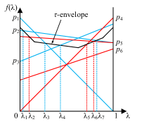
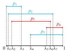
Illustration of the 2D algorithm.

3.2. Exact Two-Dimensional Algorithm

In Section 3.1, we have considered the reduction from FairHMS to interval cover and the computation of an interval for a given point $p$ and a threshold $\tau$. There are two problems remaining for an exact two-dimensional FairHMS algorithm. First, we should identify all possible values of MHRs from which the optimal one can always be found. Second, we need to determine whether a feasible interval set exists under the fairness constraint to cover the interval $[0,1]$ for a given value of MHR. Next, we present our solutions to both problems and describe our exact algorithm called IntCov for FairHMS in $\mathbb{R}^{2}_{+}$ in Algorithm 1.

Input: Dataset $\mathcal{D}\subseteq\mathbb{R}^{2}_{+}$ with $\mathcal{D}=\bigcup_{c=1}^{C}\mathcal{D}_{c}$; solution size $k\in\mathbb{Z}^{+}$; bounds $l_{1},\ldots,l_{C}\in\mathbb{Z}^{+}$ and $h_{1},\ldots,h_{C}\in\mathbb{Z}^{+}$

Output: A feasible set $S^{*}\subseteq\mathcal{D}$ for FairHMS

1 Initialize $\mathcal{H}\leftarrow\emptyset$;

2 foreach $p\in\mathcal{D}$ do

3       Add $p[1]$ and $p[2]$ to $\mathcal{H}$;

4      

5foreach $p_{i},p_{j}\in\mathcal{D}$ s.t. $p_{i}\neq p_{j}$ do

6       Let $u^{\prime}$ be the vector $u\in\mathbb{S}^{1}$ s.t. $f_{u}(p_{i})=f_{u}(p_{j})$;

7       if $u^{\prime}\in\mathbb{S}^{1}_{+}$ then

8             Add $hr(u^{\prime},\{p_{i},p_{j}\})=\frac{f_{u^{\prime}}(p_{i})}{\max_{p\in\mathcal{D}}f_{u^{\prime}}(p)}$ to $\mathcal{H}$;

9            

10      

11Sort $\mathcal{H}$ ascendingly and set $l=1,h=|\mathcal{H}|$;

12 while $\mathcal{H}[h]>\mathcal{H}[l]$ do

13       $cur=(l+h)/2$ and $\tau=\mathcal{H}[cur]$;

14       Compute $I_{\tau}(p)$ for each $p\in\mathcal{D}$;

15       $S\leftarrow$ DynProg$(\mathcal{I}_{\tau}=\{I_{\tau}(p):p\in\mathcal{D}\})$;

16       if $S=\emptyset$ then

17             $h\leftarrow cur-1$;

18            

19       else

20             $S^{*}\leftarrow S$ and $l\leftarrow cur+1$;

21            

22      

23return $S^{*}$;

Algorithm 1 IntCov

1 Create a stack $\mathcal{ST}$ and add a state $\mathtt{IC}[h_{1},\ldots,h_{C}]$ to $\mathcal{ST}$;

2 Initialize a state $\mathtt{IC}[0,\ldots,0]=0$ and set it as visited;

3 while $\mathcal{ST}\neq\emptyset$ do

4       $\mathtt{IC}[k_{1},\ldots,k_{C}]\leftarrow\mathcal{ST}$.top();

5       if $\mathtt{IC}[k_{1},\ldots,k_{C}]$ is not visited then

6             Set $\mathtt{IC}[k_{1},\ldots,k_{C}]$ as visited;

7             $\mathcal{ST}$.push$(\mathtt{IC}[k_{1},\ldots,k_{c}-1,\ldots,k_{C}])$, $\forall c\in[C]$;

8       else

9             $\mathtt{IC}[k_{1},\ldots,k_{C}]\leftarrow\mathcal{ST}$.pop();

10             if $\mathtt{IC}[k_{1},\ldots,k_{C}]$ is infeasible then

11                   continue;

12            Update $\mathtt{IC}[k_{1},\ldots,k_{C}]$ according to Equation 1;

13             if $\mathtt{IC}[k_{1},\ldots,k_{C}]=1$ then

14                   return the set $S$ w.r.t. $\mathtt{IC}[k_{1},\ldots,k_{C}]$;

15                  

16            

17      

18return $\emptyset$;

Algorithm 2 DynProg$(\mathcal{I}_{\tau})$

To resolve the first problem, i.e., finding all possible values of the MHR in $[0,1]$, we are based on an important observation from (Asudeh et al., 2017, Theorem 2) that, for any subset $S\subseteq\mathcal{D}$, $mhr(S)$ is always equal to $hr(u,S)$ for either $u=(1,0)$, or $u=(0,1)$, or the vector $u$ where $f_{u}(p_{i})=f_{u}(p_{j})$ for each pair of points $p_{i},p_{j}\in S$. Therefore, we only consider the happiness ratios of each point or pair of points in all the above cases. Specifically, we initialize an array of candidates for MHR as $\mathcal{H}=\emptyset$ (Line 1). For each $p\in\mathcal{D}$, we add $p[1]$ and $p[2]$ to $\mathcal{H}$ (Line 1). For each pair $\langle p_{i},p_{j}\rangle$ of points in $\mathcal{D}$, we compute the vector $u$ such that $f_{u}(p_{i})=f_{u}(p_{j})$. If $u\in\mathbb{S}^{1}_{+}$, we compute the value of $hr(u,\{p_{i},p_{j}\})$ and add it to $\mathcal{H}$ (Lines 1–1). Then, we sort the array $\mathcal{H}$ of size $O(n^{2})$ for binary search. For each candidate $\tau$, the interval for each point is computed according to Section 3.1, and the decision problem is solved by dynamic programming, as will be presented subsequently. Based on the answer to the decision problem, we narrow the range of the binary search by half and perform the above procedure again (Lines 1–1). After the binary search is finished, the optimal solution to FairHMS is found (Line 1).

To resolve the second problem (i.e., fair interval cover), we propose a dynamic programming algorithm in Algorithm 2. As shown in (Kleinberg and Tardos, 2006), the interval cover problem can be solved optimally by a simple greedy algorithm, which starts from an interval beginning at $0$ with the rightmost ending and then greedily adds the interval whose start point is within the covered interval and end point is the rightmost until the interval $[0,1]$ is fully covered. However, the greedy algorithm is not directly applicable to our problem because it cannot guarantee the fulfillment of the fairness constraint. Thus, we propose a dynamic program based on the greedy algorithm to solve the fair interval cover problem. We define a state $\mathtt{IC}[k_{1},\ldots,k_{C}]$ with $C$ parameters in the dynamic program, where $k_{c}$ denotes the number of tuples from $\mathcal{D}_{c}$ in the current solution, and its value is the end point of the covered interval. We use a stack $\mathcal{ST}$ in the recursive procedure to maintain and visit the states. Initially, the state $\mathtt{IC}[h_{1},\ldots,h_{C}]$ with the upper bounds of the fairness constraint is pushed to $\mathcal{ST}$ (Line 2). First, we set the start point to $0$, i.e., $\mathtt{IC}[0,\ldots,0]=0$ for an empty set $\emptyset$ with covered interval $[0,0]$ (Line 2). Then, at each step, the top state is popped from $\mathcal{ST}$. A state $\mathtt{IC}[k_{1},\ldots,k_{C}]$ is possibly transited from at most $C$ states $\mathtt{IC}[k_{1},\ldots,k_{c}-1,\ldots,k_{C}]$ for each $c\in[C]$. If $\mathtt{IC}[k_{1},\ldots,k_{C}]$ is neither the initial state nor visited, its $C$ predecessors are pushed to $\mathcal{ST}$ (Lines 2–2). Otherwise, we compute the value of $\mathtt{IC}[k_{1},\ldots,k_{C}]$ according to its predecessors by the greedy strategy (Line 2). If there is an interval $I_{\tau}(p)$ for some $c\in[C]$ and $p\in\mathcal{D}_{c}$ whose start point is at most $\mathtt{IC}[k_{1},\ldots,k_{c}-1,\ldots,k_{C}]$ and end point is the rightmost, then $\mathtt{IC}[k_{1},\ldots,k_{c},\ldots,k_{C}]$ will be set to the end point of $I_{\tau}(p)$, i.e., $p$ is added to the solution. Formally,

(1) $$\mathtt{IC}[k_{1},\ldots,k_{c},\ldots,k_{C}]=\\ \max_{c\in[C]}\Big{\{}\max_{p\in\mathcal{D}_{c}\;:\;I^{-}_{\tau}(p)\leq\mathtt{IC}[k_{1},\ldots,k_{c}-1,\ldots,k_{C}]}I^{+}_{\tau}(p)\Big{\}}$$

where $I^{-}_{\tau}(p)$ and $I^{+}_{\tau}(p)$ denote the left and right bounds of $I_{\tau}(p)$, respectively. Moreover, a state $\mathtt{IC}[k_{1},\ldots,k_{C}]$ is infeasible if $\sum_{c=1}^{C}$ $\max(l_{c},k_{c})>k$. Such a state is skipped directly because it cannot provide any feasible solution (Lines 2–2). The recursion procedure will terminate if either $\mathtt{IC}[k_{1},\ldots,k_{C}]=1$, i.e., a feasible solution that covers $[0,1]$ is found and the decision problem is answered by “yes” (Lines 2–2) or $\mathcal{ST}$ is empty and the decision problem is answered by “no” (Line 2).

Next, we will explain why our IntCov algorithm is optimal for the FairHMS problem.

Theorem 3.1.

IntCov provides an optimal solution to FairHMS.

Proof.

First, DynProg is optimal for the fair interval cover problem because (1) the recursion procedure in the dynamic program has visited all feasible group permutations to form a fair solution, and (2) the greedy strategy starting from $0$ ensures the optimality of the solution found for every group permutation. Then, the reduction from the decision version of FairHMS to the fair interval cover problem guarantees that they must have the same answer (either “yes” or “no”) for the same value of $\tau\in[0,1]$. Finally, following the analysis of (Asudeh et al., 2017; Cao et al., 2017), the array $\mathcal{H}$ has included all possible values of the optimal MHR. Given all the above results, we conclude that the output $S^{*}$ of IntCov is optimal for FairHMS. ∎

Complexity Analysis: In Algorithm 1, finding all candidates of MHR takes $O(n^{2}\log{n})$ time. Then, the binary search performs $O(\log{n})$ iterations to find the largest $\tau$. For each candidate $\tau$, computing the intervals for points in $\mathcal{D}$ takes $O(n\log{n})$ time. Algorithm 2 has at most $\prod_{c=1}^{C}{(1+h_{c})}$ states and the time to compute the value of each state is $O(n)$. Since it must hold that $h_{c}\leq k$, Algorithm 2 runs in $O(n(k^{C}+\log{n}))$ time. To sum up, the time complexity of Algorithm 1 is $O\big{(}n\log{n}(n+k^{C})\big{)}$.

4. Algorithms in MD

The FairHMS problem becomes more challenging in three and higher dimensions for its NP-hardness. Thus, we focus on efficient approximation algorithms for FairHMS on multi-dimensional datasets. Subsequently, we first introduce the background on $\delta$-net (Agarwal et al., 2017; Kumar and Sintos, 2018; Wang et al., 2021b) and the transformation from FairHMS to multi-objective submodular maximization (MOSM) (Krause et al., 2008; Anari et al., 2019; Udwani, 2018) under a matroid constraint in Section 4.1. We then present our basic algorithm BiGreedy for FairHMS based on existing methods for MOSM in Section 4.2. We further propose an adaptive sampling strategy to improve the practical efficiency of BiGreedy in Section 4.3. Note that the proofs of all lemmas are deferred to Appendix A.

4.1. Background: $\delta$-Net and Multi-Objective Submodular Maximization

The transformation from RMS to a hitting-set or set-cover problem based on the notion of $\delta$-net in (Agarwal et al., 2017; Kumar and Sintos, 2018; Wang et al., 2021b) can be similarly adapted to HMS. As shown in Section 2, the space of all utility vectors after the $l_{2}$-normalization can be denoted as the $(d-1)$-dimensional unit sphere $\mathbb{S}^{d-1}_{+}=\{u\in\mathbb{R}_{+}^{d}:||u||=1\}$. Given a parameter $\delta\in(0,1)$, a set $\mathcal{N}\subset\mathbb{S}^{d-1}_{+}$ is called a $\delta$-net (Agarwal et al., 2017) of $\mathbb{S}^{d-1}_{+}$ iff there exists a vector $v\in\mathcal{N}$ with $\langle u,v\rangle\geq\cos\delta$ for any vector $u\in\mathbb{S}^{d-1}_{+}$, where $\langle\cdot,\cdot\rangle$ is the dot product function. Intuitively, the idea of $\delta$-net is to approximate an infinite number of utility vectors in continuous space with a finite number of representative vectors such that the errors in terms of angular distances (quantified by $\cos\delta$) are bounded. A $\delta$-net of size $m=O(\frac{1}{\delta^{d-1}})$ can be computed by drawing a “uniform” grid on $\mathbb{S}^{d-1}_{+}$. A more widely used method (Saff and Kuijlaars, 1997) to compute a $\delta$-net is to sample a set of $m=O(\frac{1}{\delta^{d-1}}\log{\frac{1}{\delta}})$ vectors uniformly at random on $\mathbb{S}^{d-1}_{+}$, which will be a $\delta$-net with probability at least $1/2$. Note that the success probability of $\delta$-net computation can be arbitrarily high with repeated trials. Figure 2 illustrates a $\frac{\pi}{16}$-net in 2D by drawing $5$ vectors uniformly on $\mathbb{S}^{1}_{+}$. We adopt the random sampling method for $\delta$-net computation in our implementation. Let us define the minimum happiness ratio (MHR) of a subset $S$ over $\mathcal{D}$ on a $\delta$-net $\mathcal{N}$ of vectors as $mhr(S|\mathcal{N})=\min_{u\in\mathcal{N}}hr(u,S)$. We have the following lemma to indicate that $mhr(S|\mathcal{N})$ provides a lower bound of $mhr(S)$ with an error of at most $\frac{2\delta d}{1+\delta d}$.

Figure 2. Illustration of a $\frac{\pi}{16}$-net $\mathcal{N}$ comprised of $5$ uniform vectors $v_{1},\ldots,v_{5}$ in 2D. For any vector $u\in\mathbb{S}^{1}_{+}$, there always exists a vector (e.g., $v_{2}$) in $\mathcal{N}$ with $\langle u,v_{2}\rangle\geq\cos\frac{\pi}{16}$.

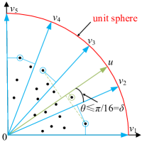
Example for delta-net

Lemma 4.1.

Given a $\delta$-net $\mathcal{N}\subset\mathbb{S}^{d-1}_{+}$, a database $\mathcal{D}$, and a subset $S\subseteq\mathcal{D}$, it holds that $mhr(S)\leq mhr(S|\mathcal{N})\leq mhr(S)+\frac{2\delta d}{1+\delta d}$.

According to Lemma 4.1, when $mhr(S)$ is estimated on a $\frac{\delta}{d(2-\delta)}$-net $\mathcal{N}\subset\mathbb{S}^{d-1}_{+}$, it holds that $mhr(S)\leq mhr(S|\mathcal{N})\leq mhr(S)+\delta$. In this way, we find an approximate solution to FairHMS by reducing it to the problem of finding a subset to maximize the MHR on a $\frac{\delta}{d(2-\delta)}$-net $\mathcal{N}$. However, although the reduced FairHMS problem is defined on a finite number of utility functions instead of an infinite utility space, it is still an NP-hard problem even without fairness constraints, as indicated in Lemma 4.2.

Lemma 4.2.

There does not exist any polynomial-time algorithm to approximate the reduced FairHMS problem defined on a set $\mathcal{N}$ of vectors in $\mathbb{S}^{d-1}_{+}$ with a factor of $(1-\varepsilon)\cdot\log{m}$, where $m=|\mathcal{N}|$, for any parameter $\varepsilon>0$ unless P=NP.

Due to the inapproximability result of reduced FairHMS, we will focus on proposing approximation algorithms within a nearly best possible factor. In Section 2, we have shown that the happiness ratio function $hr(u,\cdot)$ is monotone and submodular for any vector $u$ and the fairness constraint is a special case of matroid constraints. Therefore, the reduced FairHMS problem is an instance of maximizing the minimum of $m$ monotone submodular functions, where $m=|\mathcal{N}|$, known as the multi-objective submodular maximization (MOSM) in the literature (Krause et al., 2008; Anari et al., 2019; Udwani, 2018; Torrico et al., 2021), under a matroid constraint. Although MOSM is generally inapproximable (Krause et al., 2008), several bicriteria approximation algorithms have been proposed for MOSM under a cardinality or matroid constraint (Krause et al., 2008; Anari et al., 2019; Torrico et al., 2021). Here, an algorithm is called $(\alpha,\beta)$-bicriteria approximate for $\alpha,\beta>0$ if it provides a solution $S$ of size $\alpha k$ such that $f(S)\geq\beta f(S^{*})$, where $f$ is the minimum of $m$ monotone submodular functions and $S^{*}$ is the optimal size-$k$ solution for maximizing $f$. Next, we will generalize an existing bicriteria approximation algorithm for MOSM under a matroid constraint to FairHMS and analyze it theoretically.

The basic idea of existing algorithms is to transform the non-submodular objective function into a monotone submodular function by introducing a capped value $\tau>0$ (Fujito, 2000; Krause et al., 2008; Anari et al., 2019). Specifically, in our FairHMS problem the function $mhr(\cdot|\mathcal{N})$ is not submodular. Nevertheless, it can be transformed into a monotone submodular function as follows: First, we define a truncated happiness ratio function $hr_{\tau}(u,S)=\min\{hr(u,S),\tau\}$ for some capped value $\tau\in(0,1)$. As proven by Krause et al. (2008), for any monotone submodular function, its truncated function is monotone and submodular. Second, we define a truncated MHR function as:

(2) $$mhr_{\tau}(S|\mathcal{N})=\frac{1}{m}\sum_{u\in\mathcal{N}}hr_{\tau}(u,S)$$

where $m=|\mathcal{N}|$. Lemma 4.3 proves the soundness of truncation.

Lemma 4.3.

$mhr_{\tau}(S|\mathcal{N})$ is a monotone submodular function for any capped value $\tau\in(0,1)$.

The proof of Lemma 4.3 is trivial since $mhr_{\tau}(\cdot|\mathcal{N})$ is a nonnegative linear combination of $m$ monotone submodular functions (Krause and Golovin, 2014). Then, the reduced FairHMS problem can be regarded as a submodular maximization problem under a matroid constraint when the truncated MHR function is considered the objective function. Nevertheless, we still need to show the relationship between the truncated and original MHR functions in Lemma 4.4.

Lemma 4.4.

$mhr(S|\mathcal{N})\geq\tau$ if and only if $mhr_{\tau}(S|\mathcal{N})=\tau$.

Lemma 4.4 indicates that the truncated and original MHR functions are equivalent only when the capped value $\tau$ is achieved. And the remaining problem becomes how to find the largest $\tau$ for which there is a feasible solution $S^{*}$ under the fairness constraint with $mhr_{\tau}(S^{*}|\mathcal{N})=\tau$. In our algorithm, we attempt different values in the range $[0,1]$ so that at least one of them is near optimal with bounded error. Furthermore, to find a fair solution $S$, we adopt the greedy algorithm (Fisher et al., 1978) for submodular maximization under a matroid constraint. However, the greedy algorithm is $\frac{1}{2}$-approximate, it only guarantees to find a feasible solution $S$ with $mhr_{\tau^{*}}(S|\mathcal{N})\geq\frac{\tau^{*}}{2}$ for the optimal $\tau^{*}$ and cannot achieve any bound on $mhr(S|\mathcal{N})$. A solution to this problem is to run the greedy algorithm in $\gamma$ rounds and to take the union of the solutions $S_{1},\ldots,S_{\gamma}$ in all $\gamma$ rounds as the final solution $S=\bigcup_{i=1}^{\gamma}S_{i}$. It will lead to a solution $S$ of size $\gamma k$ that satisfies the loosened fairness constraint where all lower and upper bounds are scaled by $\gamma$ following the result in Lemma 4.5.

Lemma 4.5.

Let $\tau^{*}$ be the largest $\tau$ for which a feasible solution $S^{*}$ with $mhr_{\tau}(S^{*}|\mathcal{N})=\tau$ exists and $S_{i}$ be the solution returned by the greedy algorithm at the $i$-th round on $\mathcal{D}\setminus\bigcup_{j=1}^{i-1}S_{j}$ for function $mhr_{\tau^{*}}(\cdot|\mathcal{N})$. If $\gamma\geq\lceil\log_{2}\frac{m}{\varepsilon}\rceil$, then, for $S=\bigcup_{i=1}^{\gamma}S_{i}$, it holds that $mhr(S|\mathcal{N})\geq(1-\varepsilon)\cdot\tau^{*}$.

4.2. The BiGreedy Algorithm

Input: Dataset $\mathcal{D}\subseteq\mathbb{R}^{d}_{+}$ with $\mathcal{D}=\bigcup_{c=1}^{C}\mathcal{D}_{c}$; solution size $k\in\mathbb{Z}^{+}$; matroid $\mathcal{M}=(\mathcal{D},\mathcal{I})$; parameters $\delta,\varepsilon\in(0,1)$

Output: A feasible set $S^{\prime}\subseteq\mathcal{D}$ for FairHMS

1 Sample a $\frac{\delta}{d(2-\delta)}$-net $\mathcal{N}$ from $\mathbb{S}^{d-1}_{+}$;

2 Set $\gamma\leftarrow\lceil\log_{2}{\frac{2m}{\varepsilon}}\rceil$ where $m=|\mathcal{N}|$;

3 Initialize $\tau\leftarrow 1$ and $\mathcal{S}\leftarrow\emptyset$;

4 while $\tau\geq\frac{1}{m}$ do

5       $S\leftarrow$ MRGreedy$(\tau,\gamma,\mathcal{N},\mathcal{D})$;

6       if $S\neq\emptyset$ then

7             $\mathcal{S}\leftarrow\mathcal{S}\cup\{S\}$;

8            

9      $\tau\leftarrow(1-\frac{\varepsilon}{2})\cdot\tau$;

10      

11return $S^{\prime}\leftarrow\operatorname*{arg\,max}_{S\in\mathcal{S}}mhr(S)$;

/* Multi-Round Greedy Algorithm */

12 Function MRGreedy($\tau,\gamma,\mathcal{N},\mathcal{D}$)

13       Initialize $S\leftarrow\emptyset$ and $\mathcal{D}_{0}\leftarrow\mathcal{D}$;

14       for $i\leftarrow 1,\ldots,\gamma$ do

15             Initialize $S_{i}\leftarrow\emptyset$ and $\mathcal{D}_{i}\leftarrow\mathcal{D}_{i-1}$;

16             while there exists $p\in\mathcal{D}_{i}$ s.t. $S_{i}\cup\{p\}\in\mathcal{I}$ do

17                   $p^{*}\leftarrow\arg\max_{p\in\mathcal{D}_{i}\,:\,S_{i}\cup\{p\}\in\mathcal{I}}\Delta(p,mhr_{\tau}(S_{i}|\mathcal{N}))$;

18                   $S_{i}\leftarrow S_{i}\cup\{p^{*}\}$;

19                  

20            $S\leftarrow S\cup S_{i}$ and $\mathcal{D}_{i}\leftarrow\mathcal{D}_{i}\setminus S_{i}$;

21             if $mhr_{\tau}(S|\mathcal{N})\geq(1-\frac{\varepsilon}{2m})\cdot\tau$ then

22                   break;

23                  

24            

25      if $mhr_{\tau}(S|\mathcal{N})<(1-\frac{\varepsilon}{2m})\cdot\tau$ then

26             return $\emptyset$;

27            

28      return $S$;

29      

Algorithm 3 BiGreedy

In Lemmas 4.1–4.5, we show that the FairHMS problem can be solved as a submodular maximization problem under a matroid constraint with a bicriteria approximation guarantee, for which a multi-round greedy procedure can be used for solution computation. Accordingly, based on the above theoretical results, we propose the BiGreedy algorithm for FairHMS in Algorithm 3 algorithm. The BiGreedy algorithm uses two parameters $\delta,\varepsilon\in(0,1)$ as input to control the errors led by sampling utility vectors and searching appropriate capped values, respectively. Initially, we sample a $\frac{\delta}{d(2-\delta)}$-net $\mathcal{N}$ of $m$ utility vectors from $\mathbb{S}^{d-1}_{+}$ so that the error in the MHR estimation is bounded by $\delta$ (Line 3), as indicated by Lemma 4.1. Then, we determine that the maximum number $\gamma$ of rounds is $\lceil\log_{2}{\frac{2m}{\varepsilon}}\rceil$ to ensure that the error in the capped value is at most $\frac{\varepsilon}{2}$ (Line 3), as shown in Lemma 4.5. Next, we attempt different capped values $\tau$ in the range $[\frac{1}{m},1]$ so that at least one of them is within $[(1-\frac{\varepsilon}{2})\cdot\tau^{*},\tau^{*}]$ (Lines 3–3), where $\tau^{*}$ is the optimal capped value. For each capped value $\tau$, we run the multi-round greedy (MRGreedy) algorithm in Lines 3–3 to find a solution $S$ for FairHMS. The MRGreedy algorithm has at most $\gamma$ rounds and uses the greedy algorithm for monotone submodular maximization under a matroid constraint (Fisher et al., 1978) as a subroutine to compute a solution $S_{i}$ in the $i$-th round. At each iteration of the greedy algorithm, the point $p^{*}$ that achieves the largest marginal gain $\Delta(p,mhr_{\tau}(S_{i}|\mathcal{N}))=mhr_{\tau}(S_{i}\cup\{p\}|\mathcal{N})-mhr_{\tau}(S_{i}|\mathcal{N})$ w.r.t. the truncated MHR function and guarantees the fulfillment of the matroid constraint for group fairness in Section 2, i.e., $S_{i}\cup\{p\}\in\mathcal{I}$, is added to $S_{i}$ in the $i$-th round (Lines 3–3). After round $i$, $S_{i}$ is added to the solution $S$ of MRGreedy (Line 3). Then, we check whether $mhr_{\tau}(S|\mathcal{N})\geq(1-\frac{\varepsilon}{2m})\cdot\tau$: if yes, we will return $S$ immediately without further rounds (Line 3); otherwise, we will continue to perform the next round. If the condition is still not satisfied after all $\gamma$ rounds, an empty set will be returned by MRGreedy (Line 3). Finally, we keep all nonempty solutions returned by MRGreedy for different capped values in $\mathcal{S}$ and pick the best one with the highest $mhr(S)$ among them as the final solution $S^{\prime}$ to FairHMS (Line 3).

Next, we analyze the approximation ratio and time complexity of the BiGreedy algorithm in Theorem 4.6.

Theorem 4.6.

The BiGreedy algorithm is an $\big{(}O(d\log{\frac{1}{\delta\varepsilon}}),1-\varepsilon-\frac{\delta}{\mathtt{OPT}}\big{)}$-bicriteria approximation algorithm for the FairHMS problem, where $\mathtt{OPT}$ is the minimum happiness ratio of the optimal solution to FairHMS, running in $O\big{(}nk\varepsilon^{-2}\delta^{-d}\log^{2}{\frac{1}{\delta}}\big{)}$ time.

Proof.

First of all, we have $|S|\leq\lceil\log_{2}{\frac{2m}{\varepsilon}}\rceil\cdot k$ and $\gamma^{\prime}\cdot l_{c}\leq|S\cap\mathcal{D}_{c}|\leq\gamma^{\prime}\cdot h_{c}$ for each $c\in[C]$ because $|S_{i}|=k$ and $l_{c}\leq|S_{i}\cap\mathcal{D}_{c}|\leq h_{c}$ for each $S_{i}$ in the $i$-th round and $\gamma=\lceil\log_{2}{\frac{2m}{\varepsilon}}\rceil$, where $\gamma^{\prime}\leq\gamma$ is the practical number of rounds for the greedy algorithm. Then, let $S^{*}$ and $\mathtt{OPT}$ be the optimal solution to FairHMS and its minimum happiness ratio, respectively. According to Lemma 4.1, since $\mathcal{N}$ is a $\frac{\delta}{d(2-\delta)}$-net, we have $\mathtt{OPT}\leq mhr(S^{*}|\mathcal{N})\leq\mathtt{OPT}+\delta$. No matter what is $mhr(S^{*}|\mathcal{N})$, there always exists a capped value $\tau$ in Algorithm 3 such that $\tau\in[(1-\frac{\varepsilon}{2})\cdot mhr(S^{*}|\mathcal{N}),mhr(S^{*}|\mathcal{N})]$. For such a capped value $\tau$, its corresponding solution $S$ returned by MRGreedy satisfies that $mhr(S|\mathcal{N})\geq(1-\frac{\varepsilon}{2})\cdot\tau$ by Lemma 4.5. Therefore, we have:

$$mhr(S) \geq mhr(S|\mathcal{N})-\delta\geq(1-\varepsilon)\cdot mhr(S^{*}|\mathcal{N})-\delta$$

$$\geq(1-\varepsilon)\cdot\mathtt{OPT}-\delta=(1-\varepsilon-\frac{\delta}{\mathtt{OPT}})\cdot\mathtt{OPT}$$

Since $m=O(\delta^{-d})$, we prove that the BiGreedy algorithm is an $\big{(}O(d\log{\frac{1}{\delta\varepsilon}}),1-\varepsilon-\frac{\delta}{\mathtt{OPT}}\big{)}$-bicriteria approximation algorithm for the FairHMS problem.

In terms of time complexity, there are at most $O(\frac{\log m}{\varepsilon})$ different values of $\tau$. For each value of $\tau$, MRGreedy runs in $O(nmk\log{\frac{m}{\varepsilon}})$ time because it takes $O(nm)$ time to find $p^{*}$ per iteration and has at most $k$ iterations in $O(\log{\frac{m}{\varepsilon}})$ rounds. Therefore, the overall time complexity of BiGreedy is $O\big{(}nk\varepsilon^{-2}\delta^{-d}\log^{2}{\frac{1}{\delta}}\big{)}$. ∎

Theorem 4.6 indicates that the solution of BiGreedy is near-optimal for FairHMS when $\varepsilon$ and $\delta$ are arbitrarily small. Compared with the best possible approximation ratio, i.e., $\log{m}=O(d\log{\frac{1}{\delta}})$, the approximation ratio of BiGreedy is lowered by a factor of $O(\log{\frac{1}{\varepsilon}})$. Finally, to ensure that $S^{\prime}$ returned by BiGreedy is feasible for FairHMS (i.e., $|S^{\prime}|=k$ and $S^{\prime}\in\mathcal{I}$), we replace $k$ with $k^{\prime}=\frac{k}{\lceil\log_{2}{\frac{2m}{\varepsilon}}\rceil}$ in Algorithm 3. If the rounding errors are ignored, BiGreedy with input $k^{\prime}$ returns a feasible solution to FairHMS whose MHR is close to $\mathtt{OPT}^{\prime}$, where $\mathtt{OPT}^{\prime}$ is the optimal MHR for solution size $k^{\prime}$.

Input: Dataset $\mathcal{D}\subseteq\mathbb{R}^{d}_{+}$ with $\mathcal{D}=\bigcup_{c=1}^{C}\mathcal{D}_{c}$; solution size $k\in\mathbb{Z}^{+}$; matroid $\mathcal{M}=(\mathcal{D},\mathcal{I})$; parameters $\lambda,\varepsilon\in(0,1)$

Output: A feasible set $S^{\prime}\subseteq\mathcal{D}$ for FairHMS

1 Draw a set $\mathcal{N}_{0}$ of $m_{0}$ vectors from $\mathbb{S}^{d-1}_{+}$;

2 Run BiGreedy on $\mathcal{N}_{0}$ to get $S^{\prime}_{0}$ with capped value $\tau_{0}$;

3 for $i\leftarrow 1,\ldots,\lceil\log_{2}{\frac{M}{m_{0}}}\rceil$ do

4       Draw a set $\mathcal{N}_{i}$ of $m_{i}=2m_{i-1}$ vectors from $\mathbb{S}^{d-1}_{+}$;

5       Run BiGreedy on $\mathcal{N}_{i}$ to get $S^{\prime}_{i}$ with capped value $\tau_{i}$;

6       if $\tau_{i-1}-\tau_{i}<\lambda$ then

7             break;

8            

9      

10return $S^{\prime}\leftarrow\operatorname*{arg\,max}_{i}mhr(S^{\prime}_{i})$;

Algorithm 4 BiGreedy+

4.3. Adaptive Sampling

In this subsection, we consider an adaptive sampling strategy for $\delta$-net computation to improve the performance of the BiGreedy algorithm in practice and propose the BiGreedy+ algorithm in Algorithm 4 accordingly. The main reason why BiGreedy is not efficient in practice is the huge number $m=O(\delta^{-d})$ of vectors to form a $\frac{\delta}{d(2-\delta)}$-net $\mathcal{N}$, particularly so when $d$ is high. However, such a large sample size is often not necessary in practice. Thus, we propose an adaptive method to reduce the sample size. The basic idea is to initialize with a small size $m_{0}$ (Line 4) and run BiGreedy on a set $\mathcal{N}_{0}$ of vectors ($m_{0}=|\mathcal{N}_{0}|$) to get a solution $S^{\prime}_{0}$ with capped value $\tau_{0}$ (Line 4). Then, we double the sample size $m_{i}=2m_{i-1}$ and run BiGreedy again to get $S^{\prime}_{i}$ with capped value $\tau_{i}$ (Lines 4–4). If the capped values $\tau_{i}$ and $\tau_{i-1}$ in two consecutive rounds are close to each other (i.e., $\tau_{i-1}-\tau_{i}<\lambda$), the sample size will be regarded as large enough; otherwise, we will further increase $m$ and run BiGreedy again until $m$ exceeds a predefined limit $M$ (Lines 4–4), e.g., $M=O(\delta^{-d})$. Finally, the solution with the largest minimum happiness ratio among the ones computed in different rounds is returned as the final solution $S^{\prime}$ (Line 4). The worst-case running time of BiGreedy+ is the same as BiGreedy when $M=O(\delta^{-d})$. But its practical efficiency is significantly higher than BiGreedy because it often terminates with much smaller $m$. At the same time, its solution quality is close to that of BiGreedy in most cases, as will be shown in the experiments.

5. Experiments

In this section, we evaluate the performance of our proposed algorithms on synthetic and real-world datasets. We first introduce the experimental setup in Section 5.1. Then, the experimental results are reported in Section 5.2.

(a) Adult (Gender)

(b) Adult (Race)

(c) AntiCor_6D

(d) Compas (Gender)

(e) Credit (Job)

Figure 3. Numbers of fairness violations of different algorithms. Their original implementations without considering group fairness constraints are used for DMM, Greedy, HS, and Sphere.

experimental results

5.1. Experimental Setup

All algorithms were implemented in C++, and all experiments were conducted on a PC running Ubuntu 18.04 LTS with a 3.00GHz processor and 32GB memory. We used the CPU time of each algorithm and the minimum happiness ratios (MHRs) of their solutions as the efficiency and effectiveness measures. Furthermore, we used the number of fairness violations defined in (Halabi et al., 2020), i.e., for a given $S$,

(3) $$err(S)=\sum_{c\in[C]}\max\{|S\cap\mathcal{D}_{c}|-h_{c},l_{c}-|S\cap\mathcal{D}_{c}|,0\}$$

to measure how unfair a solution is compared to the one that satisfies the group fairness constraint.

Datasets: The experiments are conducted on one synthetic and four real-world datasets as follows.

• Anti-Correlated are synthetic datasets with $d\in\{2,\ldots,8\}$ and $n\in\{10^{2},\ldots,10^{6}\}$ created by the generator in (Börzsönyi et al., 2001). Each dataset is divided into $C\in\{2,\ldots,10\}$ groups as follows: we sort the points by the sums of their attributes and divide them into $C$ equal-sized groups accordingly. By default, we use the dataset with $d=2$ or $6$, $n=$ 10,000 and $C=3$.

• Lawschs includes 65,494 students’ information from 25 law schools from 2005 to 2007. We use two numerical attributes, namely LSAT and GPA, and two demographic attributes, namely gender and race, in our experiments.

• Adult is a 5$d$ dataset with 32,561 tuples, each of which contains an individual’s education years, capital gain, capital lose, work hours per week and overall weight. The dataset is divided into groups by gender and race.

• Compas is a 9$d$ dataset of size 4,743. It consists of customer data from an insurance company. Each tuple denotes an applicant’s insurance number of days, count of priority, comprehensive score, and so on. The dataset is partitioned by gender and whether the insured is recidivous.

• Credit is a 7$d$ dataset of 1,000 tuples about German credit information. The dataset is divided according to job, housing condition, and number of employment years.

The statistics of all the above datasets are summarized in Table 2. All the tuples in each dataset are normalized, i.e., each numerical attribute is scaled to $[0,1]$. For each dataset, the skylines are precomputed as input for each algorithm. Except for the original groups defined by one categorical attribute, we also combine several of them to form new groups. For example, the combination of gender and race forms 10 new groups in the Adult dataset.

Table 2. Statistics of datasets in the experiments. Here, #skylines is the sum of the numbers of skylines in all groups of each dataset extracted for solution computation.

Dataset	Group	$d$	$n$	$C$	#skylines
Anti-Correlated	-	$2$–$16$	$10^{2}$–$10^{6}$	$2$–$5$	$0.9n$–$n$
Lawschs	Gender	2	65,494	2	19
	Race			5	42
Adult	Gender	5	32,561	2	130
	Race			5	206
	G+R			10	339
Compas	Gender	9	4,743	2	195
	isRecid			2	229
	G+iR			4	296
Credit	Housing	7	1,000	3	120
	Job			4	126
	Working Years			5	185

(a) Lawschs (Gender)

(b) Lawschs (Race)

(c) AntiCor_2D

(d) AntiCor_2D ($k=5$)

(e) AntiCor_2D ($k=5$)

(f) Lawschs (Gender)

(g) Lawschs (Race)

(h) AntiCor_2D

(i) AntiCor_2D ($k=5$)

(j) AntiCor_2D ($k=5$)

Figure 4. Performance of different algorithms on two-dimensional datasets. In Figures (a)-(e), the MHRs of the optimal solutions without fairness constraints are plotted as black lines to illustrate the “price of fairness”.

experimental results

Algorithms: We compare the following algorithms for regret-minimizing (RMS) and happiness maximizing set (HMS) problems.

• IntCov is our exact algorithm for FairHMS on 2$d$ datasets proposed in Section 3.

• BiGreedy is our bicriteria approximation algorithm for FairHMS in Section 4.2.

• BiGreedy+ is the improved version of BiGreedy by introducing adaptive sampling in Section 4.3.

• Greedy is an RDP-Greedy algorithm for RMS in (Nanongkai et al., 2010).

• DMM is a set-cover-based RMS algorithm in (Asudeh et al., 2017).

• Sphere is an $\varepsilon$-kernel-based algorithm for RMS in (Xie et al., 2018).

• HS is a hitting-set-based RMS algorithm in (Agarwal et al., 2017; Kumar and Sintos, 2018).

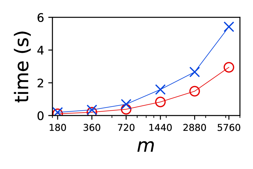
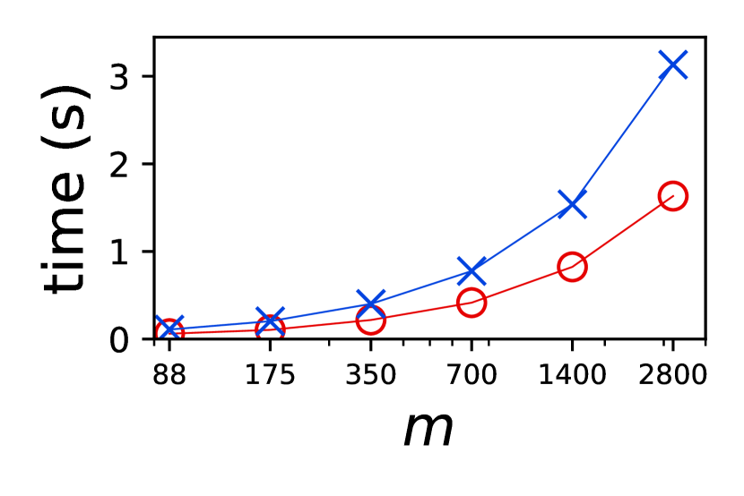
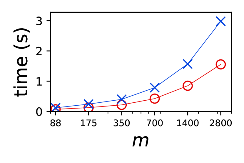
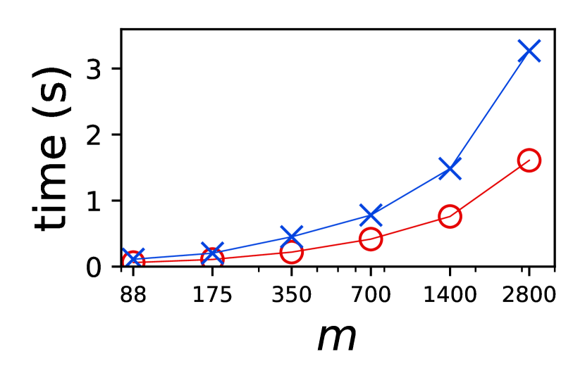
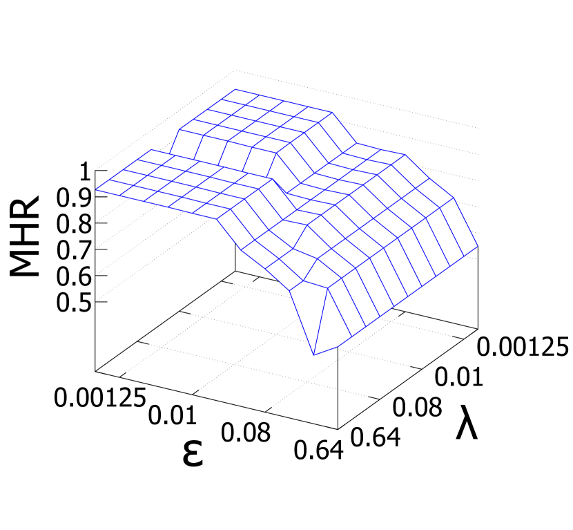
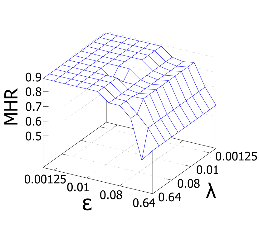
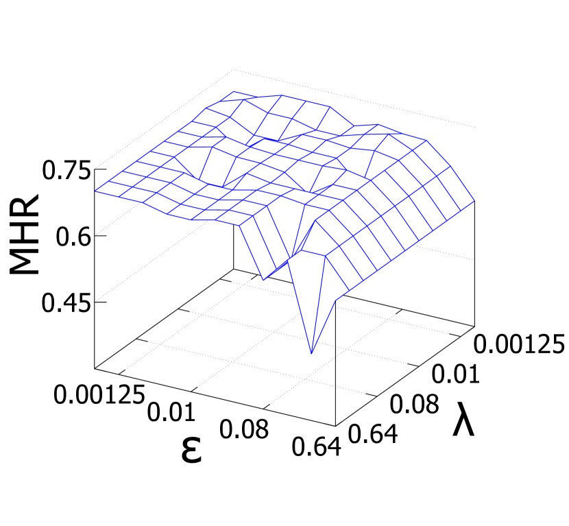
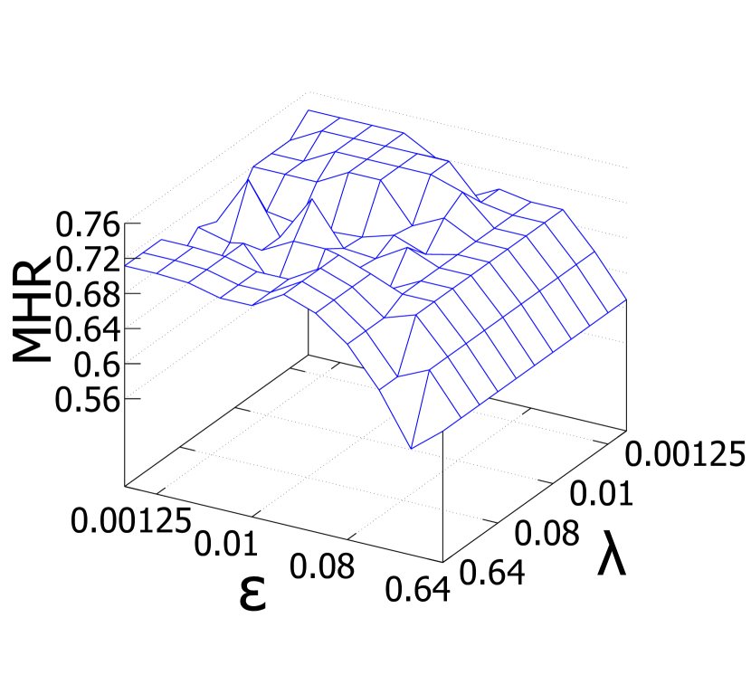
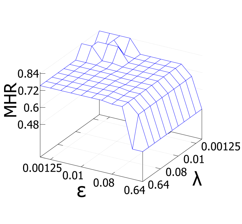
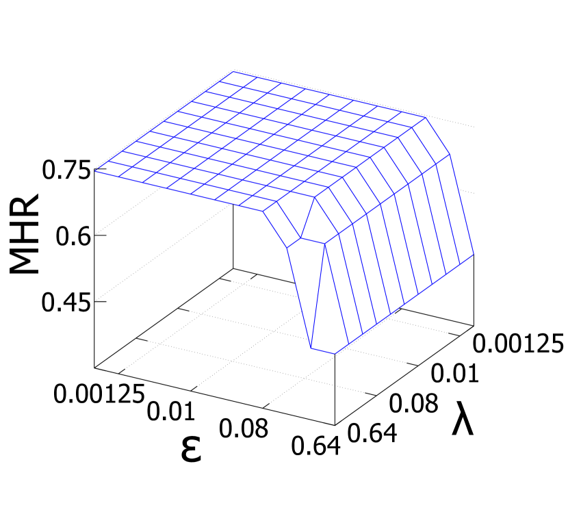
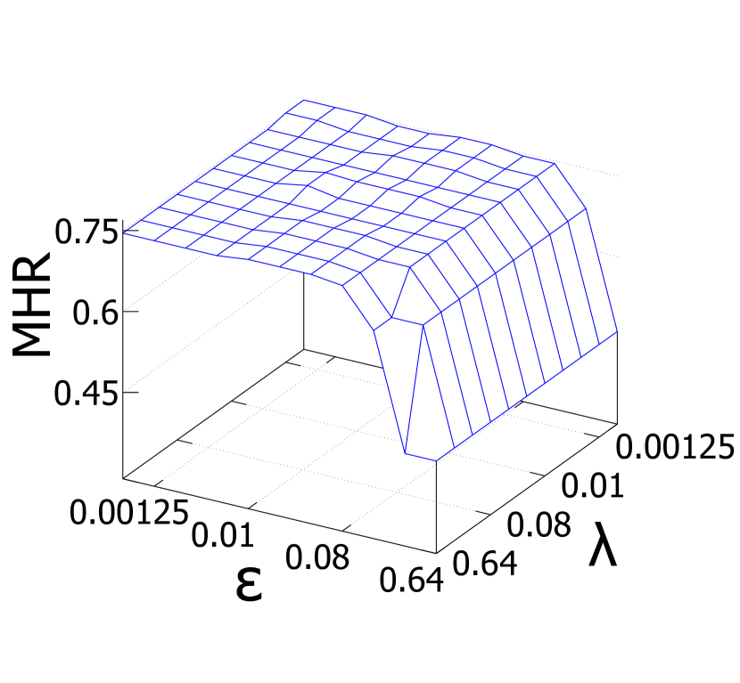
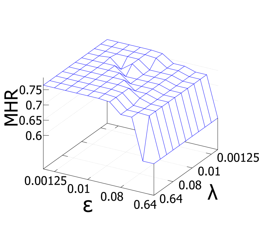
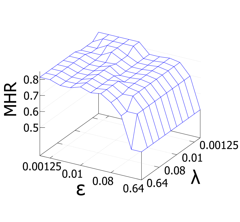
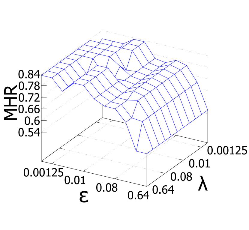
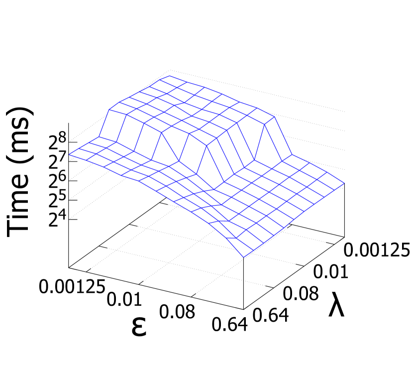
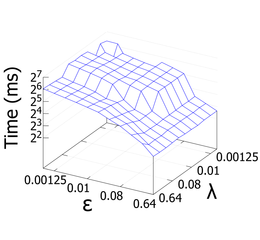
We follow the original papers to set the parameters in DMM, Sphere, and HS. For BiGreedy and BiGreedy+, we perform some preliminary experiments, which are included in Appendix B, to evaluate the effects of the values of $\delta$, $\varepsilon$, and $\lambda$. In practice, we use an increasing value of $\delta$ with $d$ to restrict the sample size $m=O(kd)$ so that BiGreedy fits in memory. The values of $m_{0}$ and $M$ in BiGreedy+ are set to $0.05m$ and $m$ accordingly. Moreover, we fix $\varepsilon=0.02,\lambda=0.04$ since using smaller $\varepsilon,\lambda$ cannot further improve the quality of solutions.

Note that all the above algorithms, except IntCov, BiGreedy, and BiGreedy+, are not designed for FairHMS. To obtain fair solutions, we run those algorithms on each group separately and take the union of the group-specific solutions as the final solution. Such an adapted version of each algorithm is referred to with a prefix ‘G-’ before its name, e.g., G-DMM for the adapted DMM. For Greedy, an alternative adaptation scheme for fairness constraints is to use the matroid greedy algorithm in (Halabi et al., 2020), which adds an item that maximally increases the MHR w.r.t. the set of selected items while ensuring the satisfaction of fairness constraint at each iteration until $k$ items are included. We refer to it as F-Greedy in the experiments. Nevertheless, to our knowledge, other algorithms cannot be adapted for fairness constraints similarly to Greedy. Also, note that none of the adapted algorithms can achieve any theoretical guarantee for FairHMS.

To verify whether these algorithms can produce fair solutions without explicitly imposing fairness constraints, we run them on the original dataset and compute the number $err(\cdot)$ of fairness violations. We use the proportional representation (Halabi et al., 2020), where the proportion of each group in the solution is approximately equal to that of the original dataset, as the fairness constraint. Specifically, we set $l_{c}$ to $\lfloor(1-\alpha)k\cdot\frac{|\mathcal{D}_{c}|}{|\mathcal{D}|}\rfloor$ or at least $1$ and $h_{c}$ to $\lceil(1+\alpha)k\cdot\frac{|\mathcal{D}_{c}|}{|\mathcal{D}|}\rceil$ or at most $k-C+1$, where $\alpha=0.1$ following (Halabi et al., 2020).

5.2. Experimental Results

(a) Adult (Gender)

(b) Adult (Race)

(c) Adult (G+R)

(d) AntiCor_6D

(e) Compas (Gender)

(f) Compas (isRecid)

(g) Compas (G+iR)

(h) Credit (Job)

(i) Credit (Housing)

(j) Credit (WY)

Figure 5. Results for the MHRs of different algorithms on multi-dimensional datasets by varying solution size $k$. In each figure, the MHRs of the best solutions without fairness constraints are plotted as black lines to illustrate the “price of fairness”.

experimental results

(a) Adult (Gender)

(b) Adult (Race)

(c) Adult (G+R)

(d) AntiCor_6D

(e) Compas (Gender)

(f) Compas (isRecid)

(g) Compas (G+iR)

(h) Credit (Job)

(i) Credit (Housing)

(j) Credit (WY)

Figure 6. Results for the running time of different algorithms on multi-dimensional datasets by varying solution size $k$.

experimental results

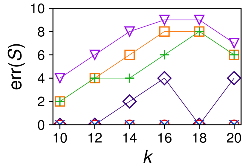
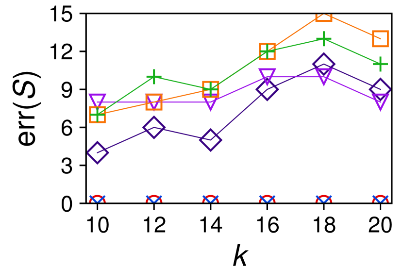
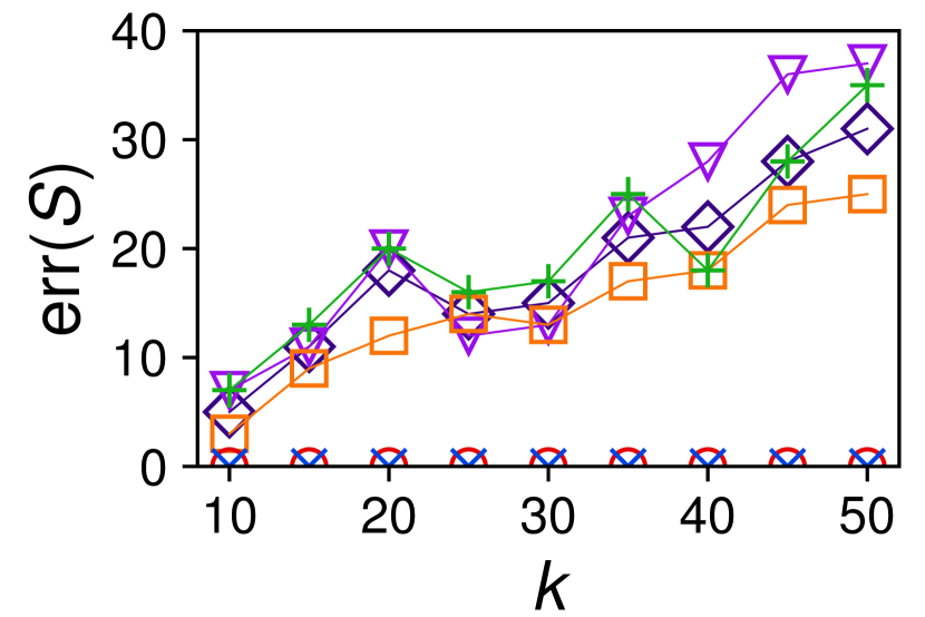
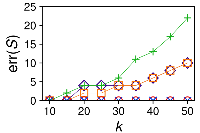
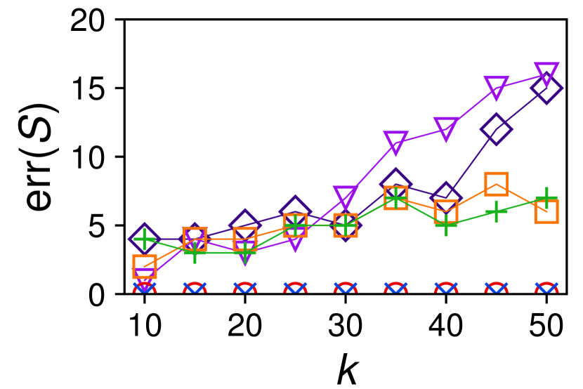
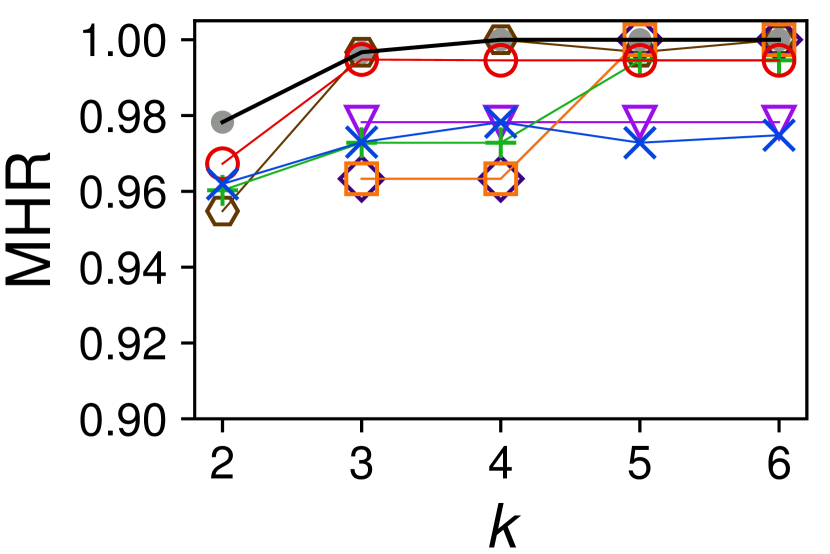
Fairness Violations: In Figure 3, we present the number of fairness violations computed by $err(S)$ in Equation 3 for the solution $S$ returned by each algorithm with varying the solution size $k$. Here, $err(S)=0$ means that $S$ satisfies the group fairness constraint, while the larger $err(S)$ is, the further away $S$ is from a fair solution. All the baseline algorithms violate the group fairness constraints in almost all cases. This is expected because their original implementations do not consider fairness; thus, their solutions show a bias towards the advantaged groups while under-representing the disadvantaged ones. Our proposed algorithms always obtain a solution with $err(S)=0$ because they strictly follow the group fairness constraint. Therefore, we will use the fair adaptations described in Section 5.1 instead of the original (unfair) implementations of the baseline algorithms in the remaining experiments.

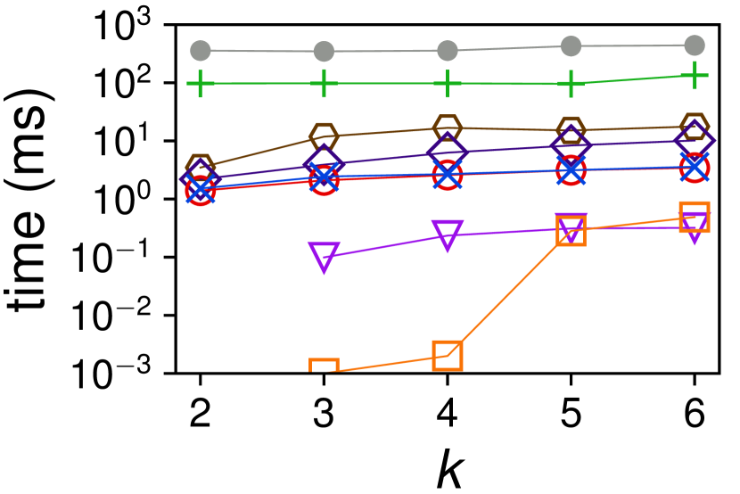
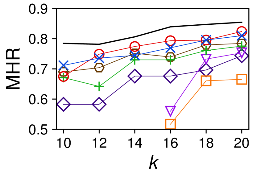
Results on Two-Dimensional Datasets: In Figure 4(j), we compare the performance of our exact IntCov algorithm and approximation BiGreedy and BiGreedy+ algorithms with the (adapted) baseline algorithms on two-dimensional datasets, i.e., Lawschs and AntiCor_2D. Note that the results of G-DMM and G-Sphere are ignored when $k$ is small or $C$ is large because they require that $k\geq d$ for computation and cannot provide any solution if there exists any $c\in[C]$ with $h_{c}<d$. In the figures for MHRs, we plot the MHRs of the optimal solutions for unconstrained HMS as black lines, from which we observe that the “price of fairness”, i.e., the decrease in MHR led by fairness constraints, is low in most cases, as the differences in MHRs between the unconstrained and fair solutions are mostly within $0.02$. Among the algorithms we compare, IntCov always obtains the highest MHRs due to its optimality. Meanwhile, it is also the slowest because of the time-consuming dynamic programming procedure. All the remaining algorithms return near-optimal solutions (MHRs $>0.9$) on Lawschs because the sizes of skylines (see Table 2) are very small. On AntiCor_2D, where the size of skylines is larger, BiGreedy and BiGreedy+ are better than the baseline algorithms in terms of the quality of solutions. In terms of time efficiency, all of the algorithms except IntCov finish within one second on all two-dimensional datasets.

In summary, IntCov provides exact solutions for FairHMS in reasonable time while BiGreedy and BiGreedy+ return solutions of better quality than the baselines with high efficiency for FairHMS on two-dimensional datasets.

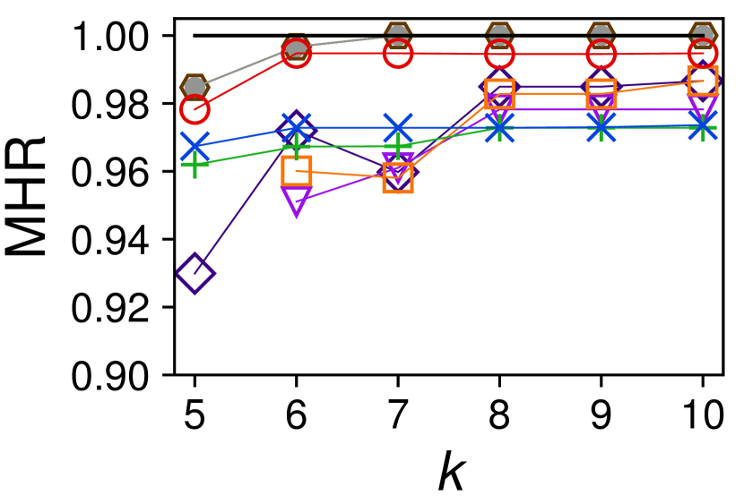
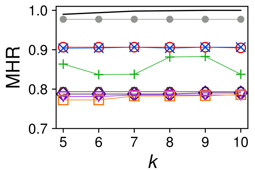
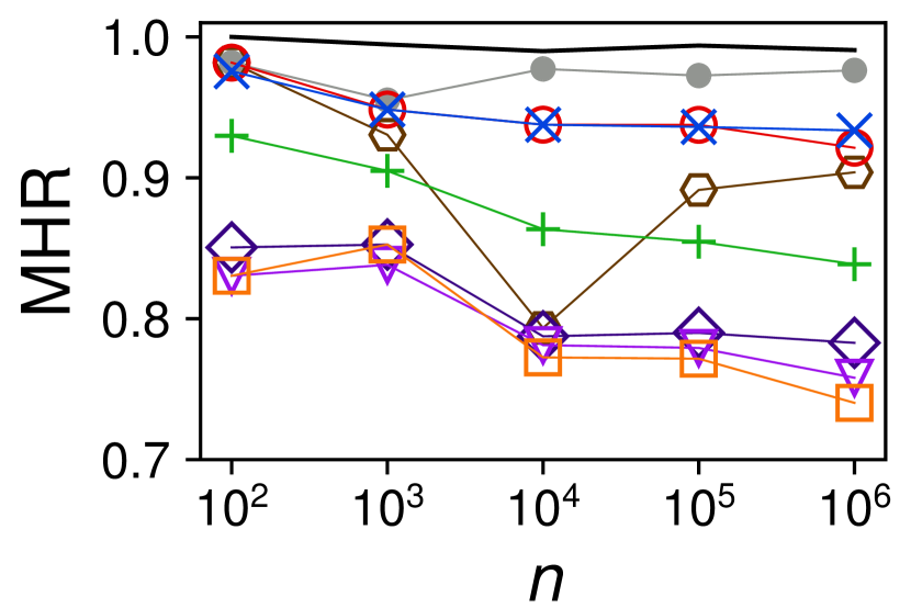
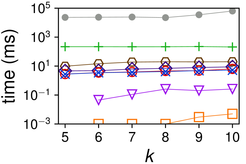
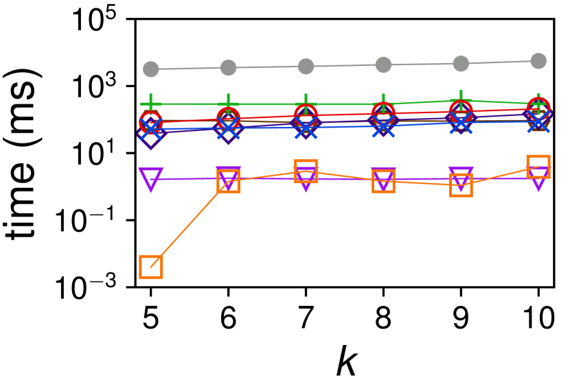
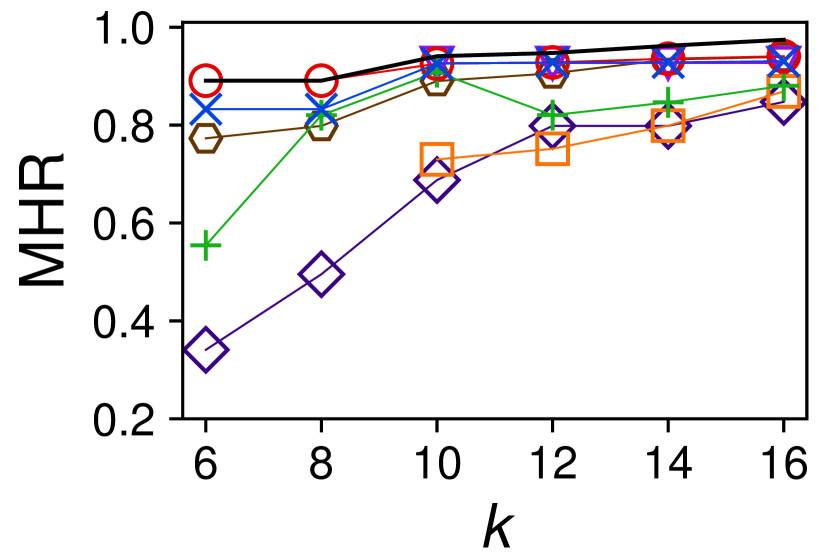
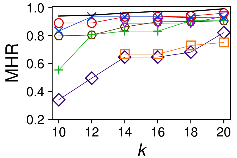
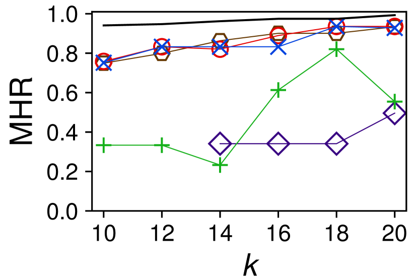
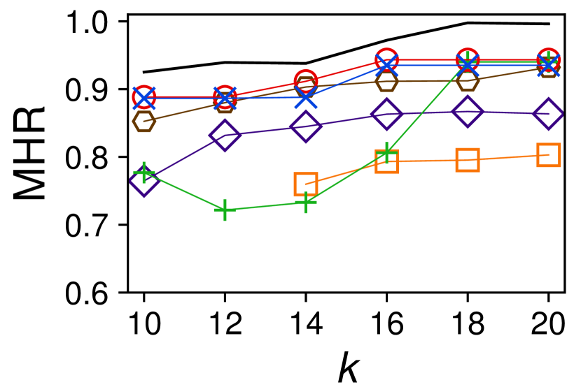
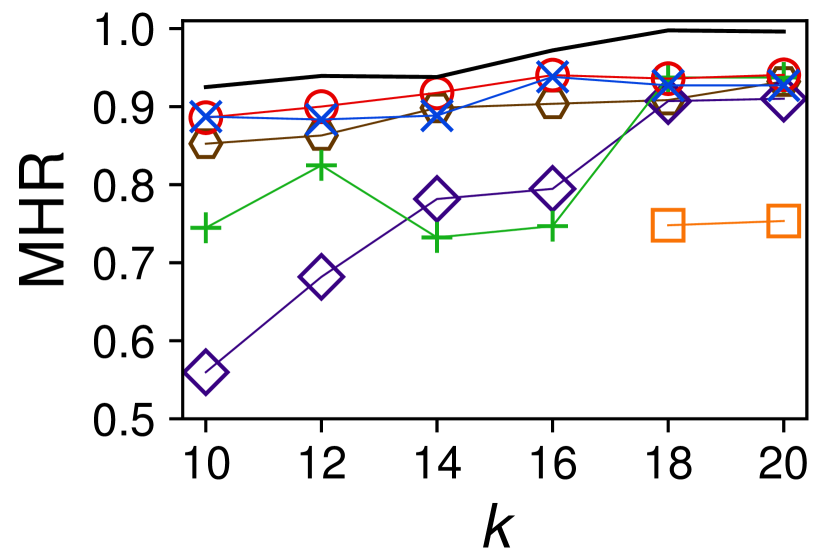
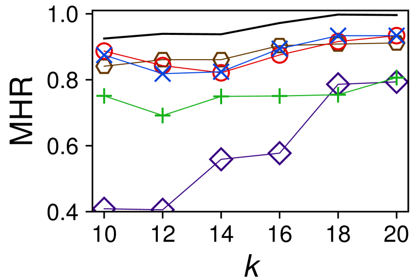
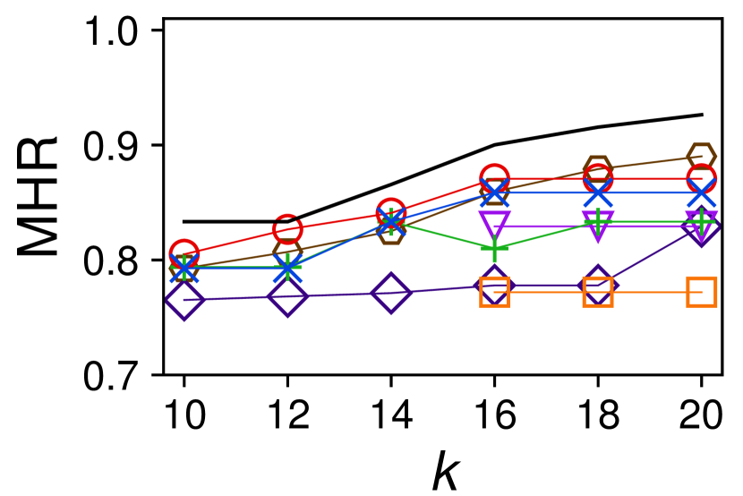
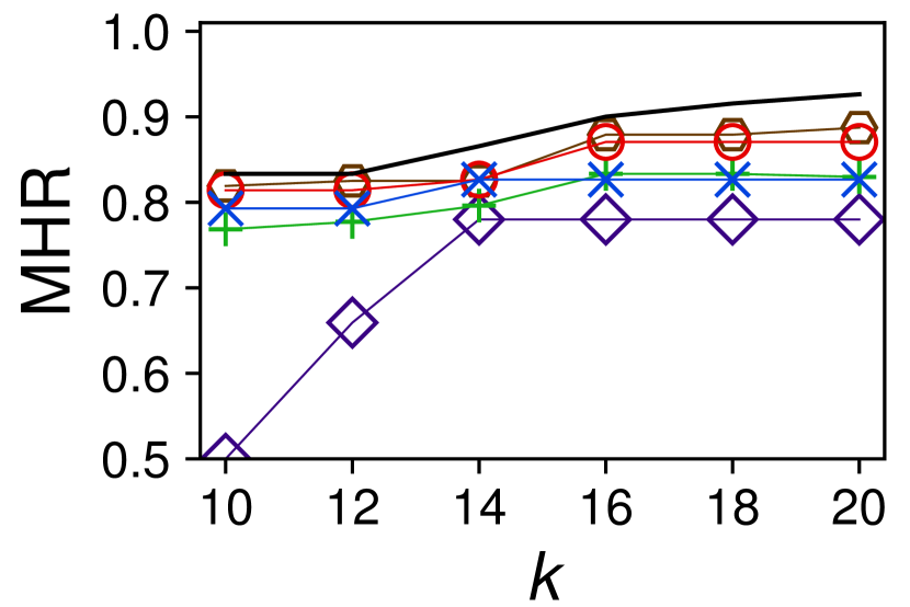
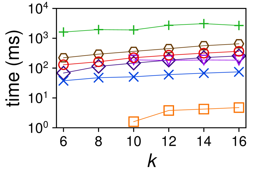
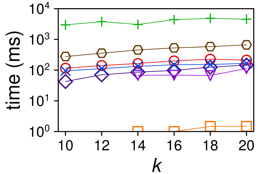
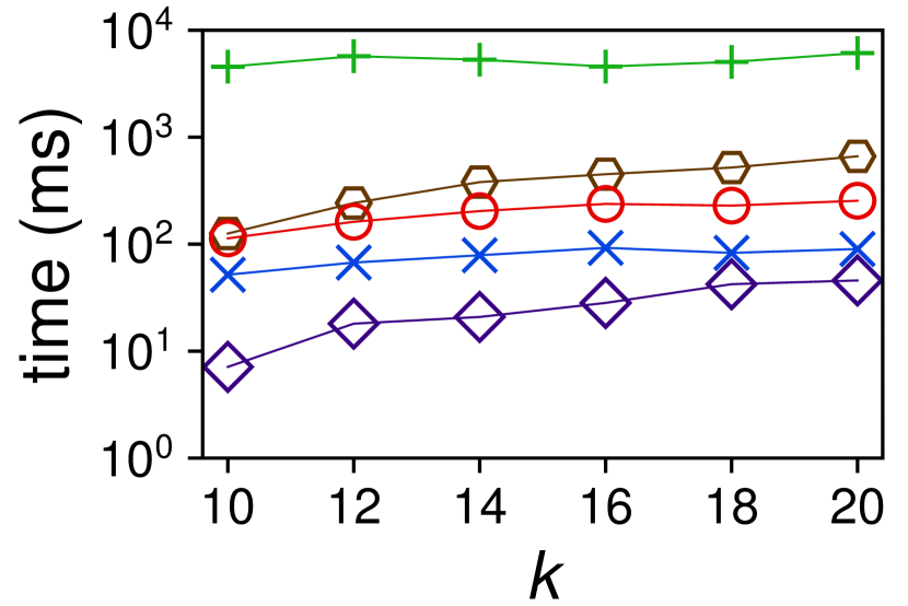
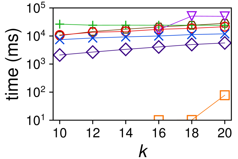
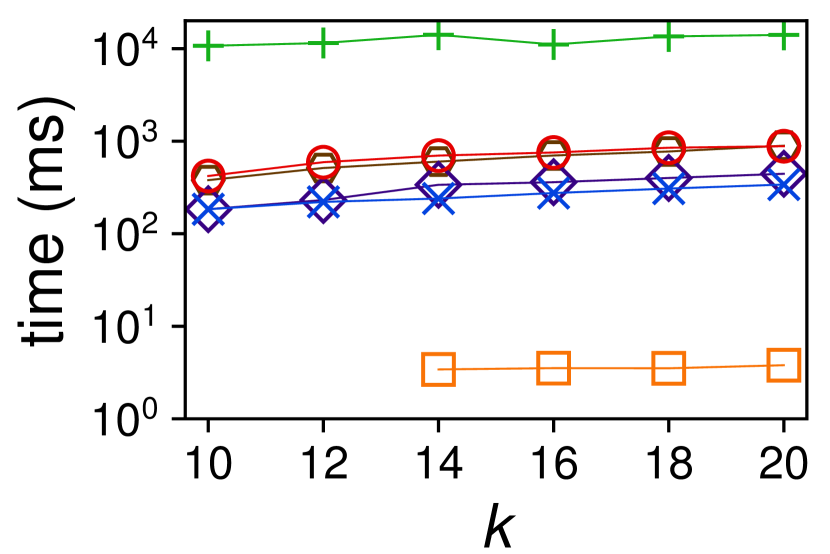
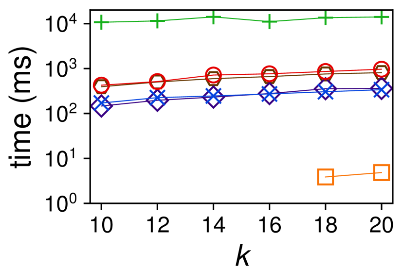
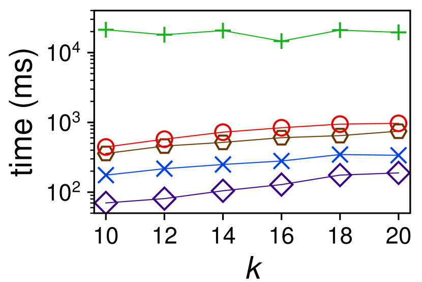
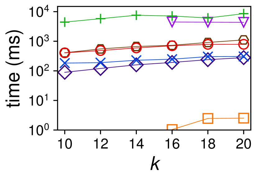
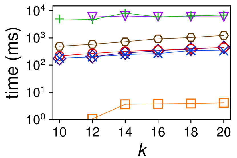
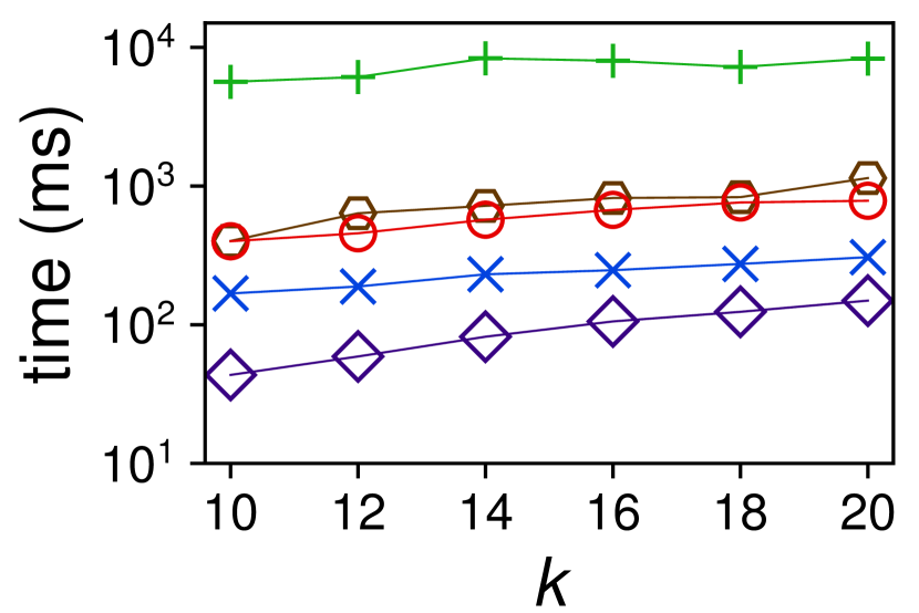
Results on Multi-Dimensional Datasets: In Figures 5(j) and 6(j), we present the MHRs and running time of different algorithms on multi-dimensional datasets, i.e., Adult, AntiCor_6D, Compas, and Credit, with different group partitions by varying the solution size $k$. We note that some results are omitted since the corresponding algorithms cannot obtain any solution. For example, DMM cannot finish when $d>7$ due to the huge memory consumption. Thus, the results of G-DMM are ignored on Compas. Moreover, as is the case for two-dimensional datasets, G-DMM and G-Sphere still cannot provide any solution if there exists any $c\in[C]$ with $h_{c}<d$.

Regarding the quality of solutions, the MHRs of all algorithms generally increase with $k$. In Figure 5(j), we plot the highest MHRs among the solutions returned by all the baseline algorithms for unconstrained HMS as black lines to illustrate the “price of fairness”. Compared with the results in 2$d$, the gaps in MHRs between unconstrained and fair solutions become larger in some cases, which may be due to two reasons. First, unconstrained solutions are merely picked from a few groups because of data skewness and thus substantially different from fair solutions. Second, unlike IntCov, the solutions of BiGreedy and BiGreedy+ are suboptimal. Furthermore, the MHRs of BiGreedy are the same as or slightly higher than those of BiGreedy+, both of which are greater than those of adapted baseline algorithms in most cases. These results confirm the effectiveness of BiGreedy and BiGreedy+ for FairHMS. We also note that in a few cases, such as Figure 5(j) (h)–(j), the MHRs of BiGreedy and BiGreedy+ are slightly lower than those of F-Greedy when $k$ is large. This is because the estimations of MHRs based on $\delta$-nets are inaccurate, as $\delta$ is too large for high dimensionality and the distributions of values for different attributes are highly skewed. In such cases, the MHR estimation using linear programs in F-Greedy is more accurate.

In terms of time efficiency, we observe that BiGreedy+ runs up to 5 times faster than BiGreedy as excepted because of smaller sample sizes for $\delta$-nets. Although several baseline algorithms, e.g., G-Sphere, G-Greedy, and G-DMM (when $d\leq 6$), run faster than BiGreedy and BiGreedy+, their solution quality is inferior to BiGreedy and BiGreedy+ in almost all cases. Since the adaptation of these algorithms for ensuring fairness constraints is merely to run one instance of the algorithm on the skylines of each group $\mathcal{D}_{c}$ with a smaller solution size $k_{c}\in[l_{c},h_{c}]$, these algorithms have little losses in efficiency due to adaptation. But their solutions may include highly redundant tuples from different groups because the selection procedures for different groups are independent of each other. Hence, they suffer from significant decreases in MHRs. Since the first step of Sphere is to select the “extreme” points with the largest attribute values in each dimension, its solution mainly consists of these extreme points when $k$ is close to $d$. For this reason, G-Sphere runs the fastest but fails to provide good solutions in almost all cases. F-Greedy runs slower than BiGreedy and BiGreedy+ in most cases. In F-Greedy, a costly linear program is executed on each item in the skyline at every iteration to find the items to add. Therefore, its running time is almost decided by the number of linear programs to execute, which is close to the original Greedy in (Nanongkai et al., 2010) and much longer than that of G-Greedy.

To sum up, BiGreedy and BiGreedy+ outperform the baseline algorithms in the quality of solutions on multi-dimensional datasets. Compared with BiGreedy, BiGreedy+ further improves the time efficiency at the expense of a bit of loss in effectiveness. Furthermore, they still only take one or several seconds for solution computation on multi-dimensional datasets.

(a) AntiCor (Varying $d$)

(b) AntiCor_6D (Varying $C$)

(c) AntiCor_6D (Varying $n$)

Figure 7. Performance of different algorithms on the anti-correlated datasets for solution size $k=20$ by varying dimensionality $d$, number of groups $C$, and dataset size $n$.

experimental results

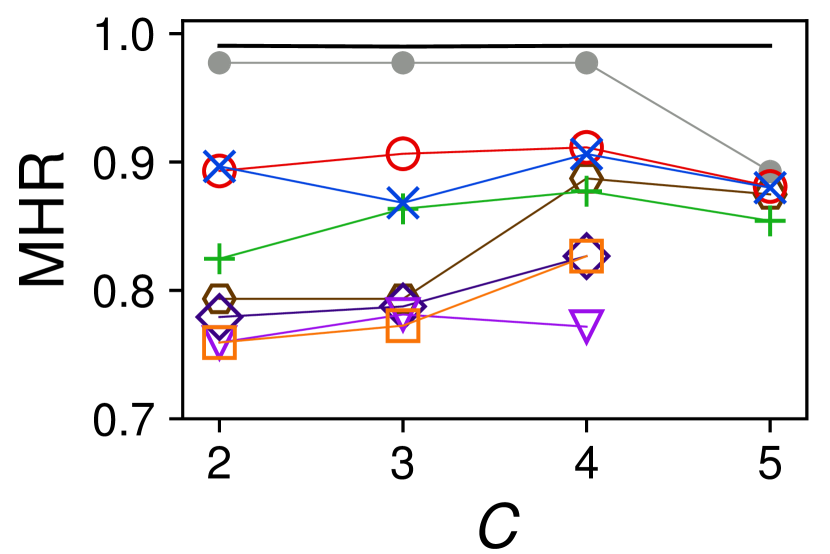
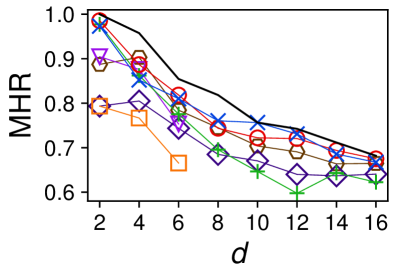
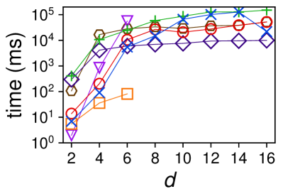
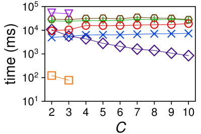
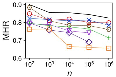
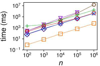
Scalability: To evaluate the scalability of different algorithms with respect to dimensionality $d$, number of groups $C$ and dataset size $n$, we perform extensive experiments on the generated anti-correlated datasets with $d$ ranging from $2$ to $8$ (with $n=10^{4}$ and $C=3$), $C$ ranging from $2$ to $10$ (with $d=2$ or $6$ and $n=10^{4}$), and $n$ ranging from $10^{2}$ to $10^{6}$ (with $d=2$ or $6$ and $C=3$). We fix the solution size $k$ to $5$ in the experiments on two-dimensional datasets only and $20$ in all remaining experiments.

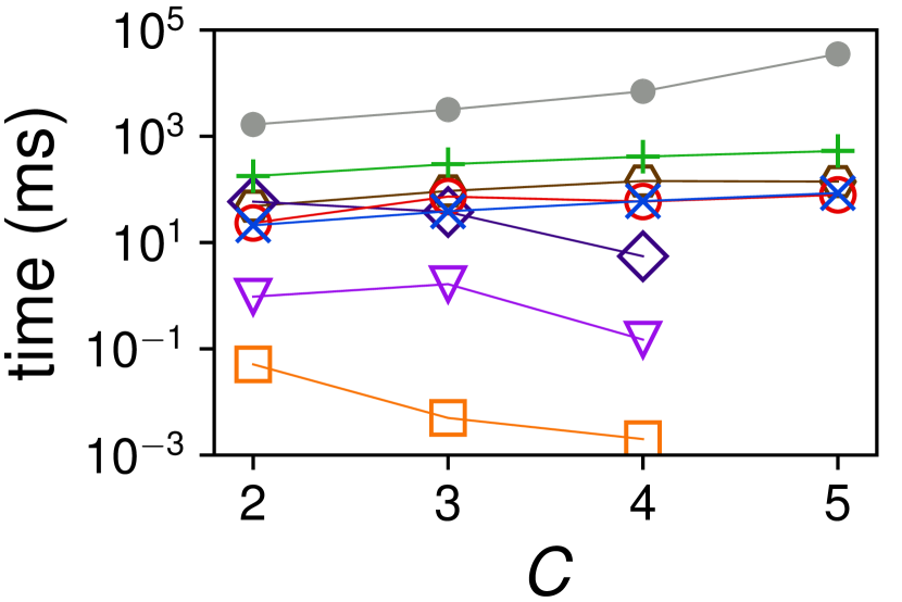
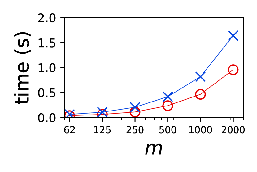
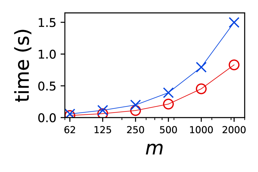
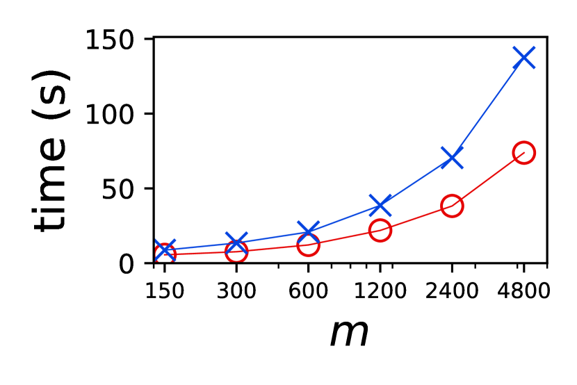
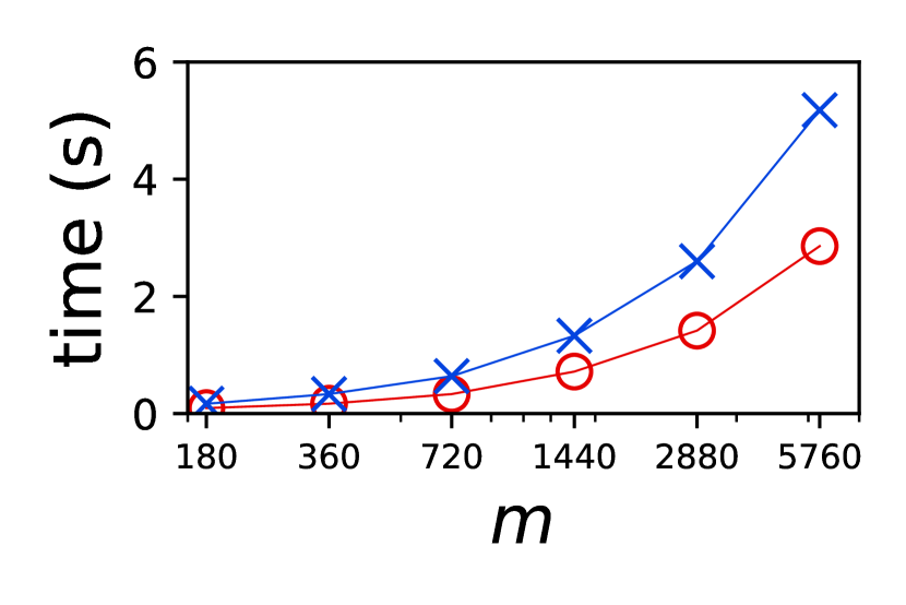
The results by varying $C$ and $n$ on 2$d$ anti-correlated datasets are presented in Figure 4(j) (d)–(e) and (i)–(j). Since the time complexity of IntCov is exponential with respect to $C$, it cannot terminate within the time limit (i.e., 1,000 seconds) when $C\geq 6$. Therefore, in the experiments, we vary $C$ from $2$ to $5$. We observe that the MHRs of different algorithms drop when $C$ increases because the fairness constraint becomes more restricted, e.g., it requires precisely one point from each group when $k=5$ and $C=5$. Nevertheless, the advantages of IntCov, BiGreedy, and BiGreedy+ remain for different values of $C$. In terms of time efficiency, unlike IntCov, BiGreedy and BiGreedy+ only run slightly slower when $C$ is larger. The running time of other algorithms drops with $C$ due to a smaller solution size for each group. Furthermore, the MHRs of all the algorithms decreases with an increasing $n$. Meanwhile, their running time increases nearly linearly with $n$. The above trends can be explained by the fact that the sizes of skylines increase proportionally with $n$ on the anti-correlated datasets. Nevertheless, IntCov, BiGreedy, and BiGreedy+ exhibit significant advantages in solution quality for different values of $n$ while the running time is still within 100 seconds for IntCov or 1 second for BiGreedy and BiGreedy+.

The results by varying $d$, $C$, and $n$ on the anti-correlated datasets of higher dimensionalities are shown in Figure 7(c). When $d$ increases, the MHR decreases while each algorithm’s running time grows drastically. For BiGreedy and BiGreedy+, the sampling sizes of $\delta$-nets grow exponentially with $d$. To achieve practical efficiency, we use larger values of $\delta$ with an increasing $d$, which inevitably leads to losses in solution quality. Other algorithms also face scalability problems due to “the curse of dimensionality”. Furthermore, when $C$ increases, the MHR decreases while the running time increases for all algorithms. The reasons for such trends are similar to those for two-dimensional data. A new observation is that the advantages of BiGreedy and BiGreedy+ over the baselines become more apparent when $C$ is larger, mainly because the solutions of baselines computed from more groups are more highly redundant. Moreover, we also observe similar trends for MHRs and running time with respect to $n$. The advantages of BiGreedy and BiGreedy+ over the baselines also become larger with an increasing $n$. Finally, the running time of all algorithms increases nearly linearly with $n$.

To sum up, BiGreedy and BiGreedy+ show better scalability than the baselines with regard to $C$ and $n$: they achieve bigger advantages in solution quality while the time efficiencies are still comparable. Moreover, they can provide solutions better than baselines in a reasonable time by adjusting the input parameters for high dimensionality $d$.

6. Related Work

RMS, HMS & Their Variants: There have been many studies on regret minimizing set (RMS) (Asudeh et al., 2017; Nanongkai et al., 2010; Peng and Wong, 2014; Shetiya et al., 2019; Xie et al., 2018), happiness maximizing set (HMS) (Qiu et al., 2018; Xie et al., 2020b), and different variants of them (Agarwal et al., 2017; Asudeh et al., 2019b; Cao et al., 2017; Chester et al., 2014; Dong and Zheng, 2019; Faulkner et al., 2015; Kumar and Sintos, 2018; Luenam et al., 2021; Nanongkai et al., 2012; Qi et al., 2018; Soma and Yoshida, 2017; Storandt and Funke, 2019; Wang et al., 2021b; Xiao and Li, 2022; Xie et al., 2019; Zeighami and Wong, 2019) (see (Xie et al., 2020a) for an extensive survey). The RMS problem was first proposed by Nanongkai et al. (2010) to alleviate the deficiencies of top-$k$ and skyline queries. Due to the NP-hardness of RMS (Agarwal et al., 2017; Cao et al., 2017; Chester et al., 2014) in three and higher dimensions, most of the literature focuses on approximation or heuristic algorithms for RMS. Nanongkai et al. (2010) first proposed a greedy heuristic for RMS. Peng and Wong (2014) devised a geometric method to improve the efficiency of the greedy heuristic. Asudeh et al. (2017) proposed an approximation algorithm for RMS by transforming it into a set cover problem. Xie et al. (2018) proposed an asymptotically optimal approximation algorithm called Sphere for RMS based on the notion of $\varepsilon$-kernels (Agarwal et al., 2004). Shetiya et al. (2019) proposed a k-medoid based heuristic algorithm for RMS. In addition, exact algorithms for RMS in $\mathbb{R}^{2}$ by transforming it into a shortest-path/cycle problem in a graph were proposed in (Asudeh et al., 2017; Wang et al., 2021c). Since minimizing the regret ratio and maximizing the happiness ratio are essentially equivalent by definition, the HMS problem was considered recently (Qiu et al., 2018; Xie et al., 2020b) in place of RMS for ease of theoretical analysis. Qiu et al. (2018) extended and improved the greedy heuristic for HMS. Xie et al. (2020b) further proposed a Cone-Greedy algorithm based on the geometric interpretation of HMS.

Different variants of RMS/HMS were also extensively studied in the literature. Chester et al. (2014) extended RMS to $k$RMS, where the notion of regret ratio was relaxed to $k$-regret ratio measuring the relative loss of the largest utility in the subset w.r.t. the $k$-th largest utility in the whole database. There have been many algorithms proposed for $k$RMS, including greedy algorithms (Chester et al., 2014; Dong and Zheng, 2019), $\varepsilon$-kernel based algorithms (Agarwal et al., 2017; Cao et al., 2017), hitting-set based algorithms (Agarwal et al., 2017; Kumar and Sintos, 2018), and fully-dynamic algorithms (Wang et al., 2021b; Zheng et al., 2022). Data reduction-based algorithms for the happiness maximization version of $k$RMS ($k$HMS) were proposed in (Luenam et al., 2021). The average RMS problem that minimizes the average instead of the maximum of regret ratios was considered in (Zeighami and Wong, 2019; Storandt and Funke, 2019; Shetiya et al., 2019, 2019). The rank-regret representative (RRR) problem, where the regret was defined by ranking other than utilities, was studied in (Asudeh et al., 2019b; Xiao and Li, 2022). The RMS problems defined on non-linear utility functions were considered in (Faulkner et al., 2015; Qi et al., 2018). Interactive RMS problems (Nanongkai et al., 2012; Xie et al., 2019; Zheng and Chen, 2020) were proposed to enhance RMS with user interactions.

However, despite the rich literature on RMS/HMS, none of the above studies have taken fairness into consideration. They could provide solutions that under-represent some protected groups, as already shown in our experiments, and might further lead to bias and discrimination in algorithmic decisions.

Fairness in Subset Selection and Ranking: Another line of work related to ours is subset selection and ranking under fairness constraints. The relationship between this work and existing fair subset selection problems is that the notions of fairness are the same or similar. Specifically, the group fairness constraint in this work and its special case when the upper and lower bounds are equal to each other have been used in many real-world problems, including DPP-based data summarization (Celis et al., 2018b), $k$-center clustering (Kleindessner et al., 2019), top-$k$ selection (Stoyanovich et al., 2018; Mehrotra and Celis, 2021), submodular maximization (Wang et al., 2021a; Halabi et al., 2020; Celis et al., 2018a), diversity maximization (Moumoulidou et al., 2021). However, since the objective function of HMS is not submodular in its original form, existing algorithms for fair submodular maximization cannot be directly used for FairHMS. Moreover, as they only consider a single utility function, the fair top-$k$ selection algorithms are also not applicable to FairHMS. Finally, the inner product-based objective of HMS essentially differs from the distance-based objectives in summarization, clustering, and diversification, and thus the design of algorithms for the fair variants of these problems are very different from that for FairHMS.

Ranking problems under fairness constraints are also attracting much attention recently (see (Pitoura et al., 2022; Zehlike et al., 2021) for extensive surveys). Zehlike et al. (2017) and Celis et al. (2018c) generalized the fairness constraints for top-$k$ selection to top-$k$ ranking by further restricting that every prefix of the ranking should also be proportionally fair. Singh and Joachims (2018) defined fairness constraints on rankings in terms of exposure allocation based on the notion of discounted cumulative gain (DCG). García-Soriano and Bonchi (2021) designed a maximin-fair ranking framework to achieve individual fairness under group-fairness constraints. Asudeh et al. (2019a) proposed a scheme to modify a ranking function towards satisfying the desired fairness constraints. Kuhlman and Rundensteiner (2020) considered how to aggregate multiple rankings under fairness constraints. Unlike subset selection, the concepts of fairness in ranking problems consider not only whether a tuple is picked but also its position in the result. Since HMS is not ordered, the fairness constraints designed for ranking problems are not applicable for FairHMS.

7. Conclusion

In this paper, we studied the problem of happiness maximizing sets under group fairness constraints (FairHMS). We first formally defined the FairHMS problem and showed its NP-hardness in three and higher dimensions. Then, we proposed an exact algorithm for FairHMS on two-dimensional data. Moreover, we proposed a bicriteria approximation algorithm for FairHMS in any constant dimension based on the notion of $\delta$-nets and multi-objective submodular maximization. We further introduced an adaptive sampling strategy to improve its practical efficiency. Finally, extensive experiments on real-world and synthetic datasets confirmed the efficacy, efficiency, and scalability of our proposed algorithms.

(a) Adult (Gender)

(b) Adult (Race)

(c) Adult (G+R)

(d) AntiCor_6D

(e) Compas (Gender)

(f) Compas (isRecid)

(g) Compas (G+iR)

(h) Credit (Job)

(i) Credit (Housing)

(j) Credit (WY)

Figure 8. Results for the MHRs of BiGreedy and BiGreedy+ by varying sample size $m$ or maximum sample size $M$.

experimental results

(a) Adult (Gender)

(b) Adult (Race)

(c) Adult (G+R)

(d) AntiCor_6D

(e) Compas (Gender)

(f) Compas (isRecid)

(g) Compas (G+iR)

(h) Credit (Job)

(i) Credit (Housing)

(j) Credit (WY)

Figure 9. Results for the running time of BiGreedy and BiGreedy+ by varying sample size $m$ or maximum sample size $M$.

experimental results

Appendix A Missing Proofs

In this section, we provide the proofs of theorems and lemmas omitted from the paper.

A.1. Proof of Lemma 4.1

Lemma 4.1.  Given a $\delta$-net $\mathcal{N}\subset\mathbb{S}^{d-1}_{+}$, a database $\mathcal{D}$, and a subset $S\subseteq\mathcal{D}$, it holds that $mhr(S)\leq mhr(S|\mathcal{N})\leq mhr(S)+\frac{2\delta d}{1+\delta d}$.

Proof.

First of all, since $\mathcal{N}\subset\mathbb{S}^{d-1}_{+}$, it is obvious that $mhr(S)=\min_{u\in\mathbb{S}^{d-1}_{+}}hr(u,S)\leq\min_{u\in\mathcal{N}}hr(u,S)=mhr(S|\mathcal{N})$. Then, it suffices to show that $mhr(S|\mathcal{N})\leq mhr(S)+\frac{2\delta d}{1+\delta d}$. For any vector $u\in\mathbb{S}^{d-1}_{+}$, there exists a vector $v\in\mathcal{N}$ with $\langle u,v\rangle\geq\cos\delta$ by the definition of $\delta$-net and we get

$$\|u-v\| =\sqrt{\sum_{i=1}^{d}(u[i]-v[i])^{2}}=\sqrt{2-2\sum_{i=1}^{d}u[i]\cdot v[i]}$$

$$\leq\sqrt{2-\cos\delta}=2\sin(\delta/2)\leq\delta$$

based on trigonometric equations. For any point $p\in[0,1]^{d}$, according to the Cauchy-Schwarz inequality (Agarwal et al., 2017; Wang et al., 2021b), we have

(4) $$|\langle u,p\rangle-\langle v,p\rangle|\leq\|u-v\|\cdot\|p\|\leq\delta\|p\|\leq\delta\sqrt{d}$$

Thus, for any subset $S\subseteq\mathcal{D}$, we suppose that the MHR of $S$ over $\mathcal{D}$ is reached on vector $u^{\prime}$, i.e., $u^{\prime}=\operatorname*{arg\,min}_{u\in\mathbb{S}^{d-1}_{+}}hr(u,S)$ and there is a vector $v^{\prime}\in\mathcal{N}$ with $\langle u^{\prime},v^{\prime}\rangle\geq\cos\delta$. By adapting the analysis in (Agarwal et al., 2017; Wang et al., 2021b) from RMS to HMS, we have the following results for the vectors $u^{\prime}$ and $v^{\prime}$:

$$mhr(S) =\frac{\max_{p\in S}\langle u^{\prime},p\rangle}{\max_{p\in\mathcal{D}}\langle u^{\prime},p\rangle}\geq\frac{\max_{p\in S}\langle v^{\prime},p\rangle-\delta\sqrt{d}}{\max_{p\in\mathcal{D}}\langle v^{\prime},p\rangle+\delta\sqrt{d}}$$

$$\geq\frac{mhr(S|\mathcal{N})-\frac{\delta\sqrt{d}}{\max_{p\in\mathcal{D}}\langle v^{\prime},p\rangle}}{1+\frac{\delta\sqrt{d}}{\max_{p\in\mathcal{D}}\langle v^{\prime},p\rangle}}\geq\frac{mhr(S|\mathcal{N})-\delta d}{1+\delta d}$$

$$\geq mhr(S|\mathcal{N})-\frac{2\delta d}{1+\delta d}$$

where the first inequality is based on Equation 4, the second inequality is obtained from the fact that $mhr(S|\mathcal{N})\leq\frac{\max_{p\in S}\langle v^{\prime},p\rangle}{\max_{p\in\mathcal{D}}\langle v^{\prime},p\rangle}$, the third inequality is because $\max_{p\in\mathcal{D}}\langle v^{\prime},p\rangle\geq 1/\sqrt{d}$, and the fourth inequality is acquired from $mhr(S|\mathcal{N})\leq 1$. ∎

A.2. Proof of Lemma 4.2

Lemma 4.2.  There does not exist any polynomial-time algorithm to approximate the reduced FairHMS problem defined on a set $\mathcal{N}$ of vectors in $\mathbb{S}^{d-1}_{+}$ with a factor of $(1-\varepsilon)\cdot\log{m}$, where $m=|\mathcal{N}|$, for any parameter $\varepsilon>0$ unless P=NP.

Proof.

We prove this theorem by reducing from the SetCover problem, a classic NP-Hard problem (Feige, 1998), to the reduced FairHMS problem when $C=1$ (i.e., without fairness constraints). Given a ground set $\mathcal{E}=\{e_{1},\ldots,e_{m}\}$, a set collection $\mathcal{S}=\{S_{1},\ldots,S_{n}\}$ where $S_{j}\subseteq\mathcal{E}$, the SetCover decision problem is to determine whether there exists a size-$k$ subset $\mathcal{S}^{\prime}\subseteq\mathcal{S}$ such that $\bigcup_{S\in\mathcal{S}^{\prime}}S=\mathcal{E}$. Then, for each element $e_{i}\in\mathcal{E}$, we define an $m$-dimensional unit vector $u_{i}=(u_{i}[1],\ldots,u_{i}[m])$, where $u_{i}[j]=1$ if $i=j$ and $u_{i}[j]=0$ otherwise for each $i,j\in[1,m]$. For each set $S_{j}\in\mathcal{S}$, we define an $m$-dimensional point $p_{j}=(p_{j}[1],\ldots,p_{j}[m])$ where $p_{j}[i]=1$ if $e_{i}\in S_{j}$ and $p_{j}[i]=0$ otherwise for each $i\in[1,m]$ and $j\in[1,n]$. Intuitively, if a sub-collection $\mathcal{S}^{\prime}$ covers $u_{i}$, there will exist a point $p$ w.r.t. some $S\in\mathcal{S}^{\prime}$ such that $\langle p,u_{i}\rangle=1$ and vice versa. In this way, we reduce a SetCover instance on $\mathcal{E}$ and $\mathcal{S}$ to an HMS instance on $U=\{u_{i}:i\in[1,m]\}$ and $\mathcal{D}=\{p_{j}:j\in[1,n]\}$. Next, we show that there exists a sub-collection $\mathcal{S}^{\prime}$ of $k$ sets to cover $\mathcal{E}$ if and only if the minimum happiness ratio $mhr(P|U)$ of the size-$k$ point set $P$ corresponding to $\mathcal{S}^{\prime}$ defined on $U$ is $1$.

• If Direction: If $mhr(P|U)=1$, there exists a point $p_{j}\in P$ such that $\langle p_{j},u_{i}\rangle=1$ for any $u_{i}\in U$ and thus $p_{j}[i]=1$, which implies that there is a set $S_{j}\in\mathcal{S}^{\prime}$ such that $e_{i}\in S_{j}$ for every $e_{i}\in\mathcal{E}$. Thus, $\mathcal{S}^{\prime}$ is a solution for the SetCover problem.

• Only if Direction: If $\bigcup_{S\in\mathcal{S}^{\prime}}S=\mathcal{E}$, then, for each $u_{i}\in U$, there is a set $S_{j}\in\mathcal{S}^{\prime}$ whose corresponding point $p_{j}$ satisfies that $\langle p_{j},u_{i}\rangle=1$. Moreover, since $\max_{p\in\mathcal{D}}\langle p,u_{i}\rangle=1$ for any $u_{i}\in U$, we get $hr(u_{i},P)=1/1=1$ and thus $mhr(P)=1$, where $P=\{p_{j}:S_{j}\in\mathcal{S}^{\prime}\}$.

Since the above reduction procedure is performed in $O(nm)$ time, we prove that HMS is NP-hard from the NP-hardness of SetCover. Because HMS is a special case of FairHMS when $C=1$, the reduced FairHMS problem is NP-hard as well. Furthermore, it is known that there does not exist any polynomial-time algorithm that approximates the SetCover problem within a factor of $(1-\varepsilon)\log m$ for any $\varepsilon>0$ unless $\mathrm{NP}\subset\mathrm{TIME}(n^{O(\log{\log n})})$ ((Feige, 1998), Theorem 4.4). Formally, suppose that $\mathcal{S}^{*}$ be the smallest sub-collection of $\mathcal{S}$ that covers $\mathcal{E}$, no polynomial-time algorithm can guarantee to find a sub-collection of $\mathcal{S}^{\prime}$ that covers $\mathcal{E}$ with $|\mathcal{S}^{\prime}|\leq(1-\varepsilon)\log m\cdot|\mathcal{S}^{*}|$ for any $\varepsilon>0$ unless P=NP. The hardness result holds for HMS/FairHMS as well, i.e., there is no polynomial-time algorithm that guarantees to find a solution $S_{\tau}$ of size $k_{\tau}=(1-\varepsilon)\log m\cdot k^{*}_{\tau}$ for any $\varepsilon>0$ with $mhs(S_{\tau})=\tau$ unless P=NP, where $k^{*}_{\tau}$ is the size of the smallest subset $S^{*}_{\tau}$ for HMS with $mhs(S^{*}_{\tau})=\tau$ for any $\tau\in(0,1)$. ∎

A.3. Proof of Lemma 4.4

Lemma 4.4.  $mhr(S|\mathcal{N})\geq\tau$ if and only if $mhr_{\tau}(S|\mathcal{N})=\tau$.

Proof.

On the one hand, since $\min_{u\in\mathcal{N}}hr(u,S)\geq\tau$, we have $hr_{\tau}(u,S)=\tau$ for any $u\in\mathcal{N}$ and thus $mhr_{\tau}(S|\mathcal{N})=\frac{m\tau}{m}=\tau$.

On the other hand, we assume that there exists some $u^{\prime}\in\mathcal{N}$ such that $hr(u^{\prime},S)<\tau$ and thus $hr_{\tau}(u^{\prime},S)=\min\{hr(u^{\prime},S),\tau\}<\tau$. Since $hr_{\tau}(u,S)\leq\tau$, $mhr_{\tau}(S|\mathcal{N})\leq\frac{(m-1)\tau+hr(u^{\prime},S)}{m}<\tau$, which contradicts with $mhr_{\tau}(S|\mathcal{N})=\tau$. Hence, we will have $hr(u,S)\geq\tau$ for each $u\in\mathcal{N}$ and $mhr(S|\mathcal{N})\geq\tau$ if $mhr_{\tau}(S|\mathcal{N})=\tau$. ∎

A.4. Proof of Lemma 4.5

Lemma 4.5.  Let $\tau^{*}$ be the largest $\tau$ for which a feasible solution $S^{*}$ with $mhr_{\tau}(S^{*}|\mathcal{N})=\tau$ exists and $S_{i}$ be the solution returned by the greedy algorithm at the $i$-th round on $\mathcal{D}\setminus\bigcup_{j=1}^{i-1}S_{j}$ for function $mhr_{\tau^{*}}(\cdot|\mathcal{N})$. If $\gamma\geq\lceil\log_{2}\frac{m}{\varepsilon}\rceil$, then, for $S=\bigcup_{i=1}^{\gamma}S_{i}$, it holds that $mhr(S|\mathcal{N})\geq(1-\varepsilon)\cdot\tau^{*}$.

Proof.

First, according to Theorem 3 of (Anari et al., 2019) generalizing from the statement in (Fisher et al., 1978), we have

$$mhr_{\tau^{*}}(S|\mathcal{N})\geq(1-2^{-\gamma})\cdot\tau^{*}\geq(1-\frac{\varepsilon}{m})\cdot\tau^{*}$$

Suppose that there exists some $u\in\mathcal{N}$ s.t. $hr_{\tau^{*}}(u,S)$ $<(1-\varepsilon)\cdot\tau^{*}$. Because it is known that $hr_{\tau^{*}}(u,S)\leq\tau^{*}$ for every $u\in\mathcal{N}$, we have

$$mhr_{\tau}(S|\mathcal{N}) \leq\frac{1}{m}\cdot hr_{\tau^{*}}(u,S)+\frac{m-1}{m}\cdot\tau^{*}$$

$$<\frac{1-\varepsilon}{m}\cdot\tau^{*}+\frac{m-1}{m}\cdot\tau^{*}=(1-\frac{\varepsilon}{m})\cdot\tau^{*}$$

which contradicts with $mhr_{\tau^{*}}(S|\mathcal{N})\geq(1-\frac{\varepsilon}{m})\cdot\tau^{*}$. Therefore, we have $hr_{\tau^{*}}(u,S)\geq(1-\varepsilon)\cdot\tau^{*}$ for $u\in\mathcal{N}$ and thus $mhr(S|\mathcal{N})\geq(1-\varepsilon)\cdot\tau^{*}$ as claimed. ∎

(a) Adult (Gender)

(b) Adult (Race)

(c) Adult (G+R)

(d) AntiCor_6D

(e) Compas (Gender)

(f) Compas (isRecid)

(g) Compas (G+iR)

(h) Credit (Job)

(i) Credit (Housing)

(j) Credit (WY)

Figure 10. Results for the MHRs of BiGreedy+ by varying $\varepsilon$ and $\lambda$.

experimental results

(a) Adult (Gender)

(b) Adult (Race)

(c) Adult (G+R)

(d) AntiCor_6D

(e) Compas (Gender)

(f) Compas (isRecid)

(g) Compas (G+iR)

(h) Credit (Job)

(i) Credit (Housing)

(j) Credit (WY)

Figure 11. Results for the running time of BiGreedy+ by varying $\varepsilon$ and $\lambda$.

experimental results

Appendix B Additional Experiments

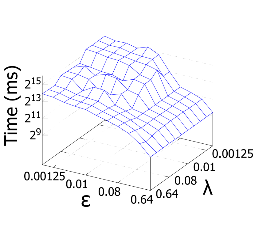
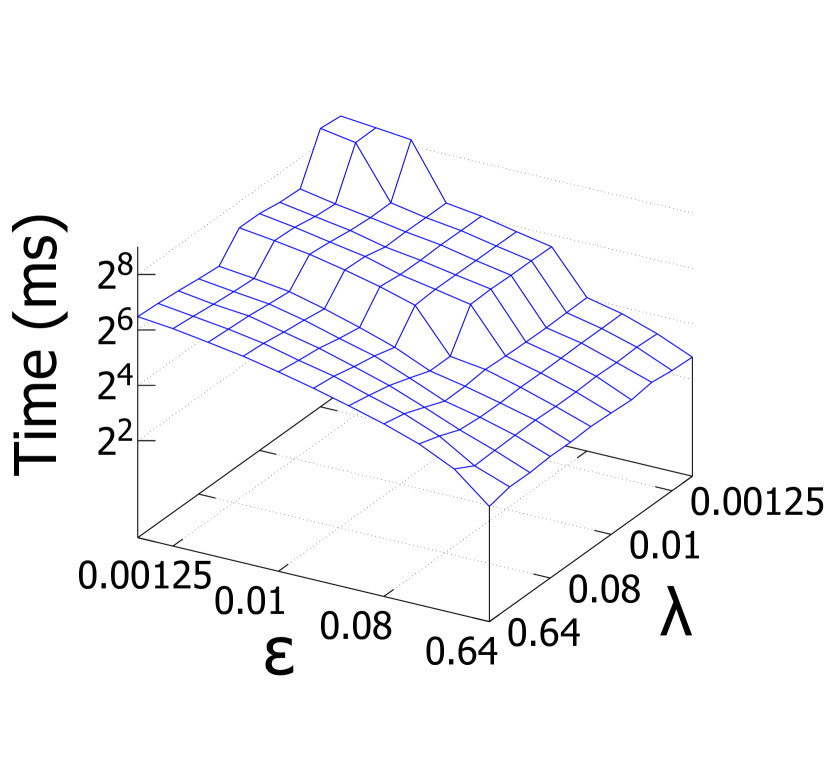
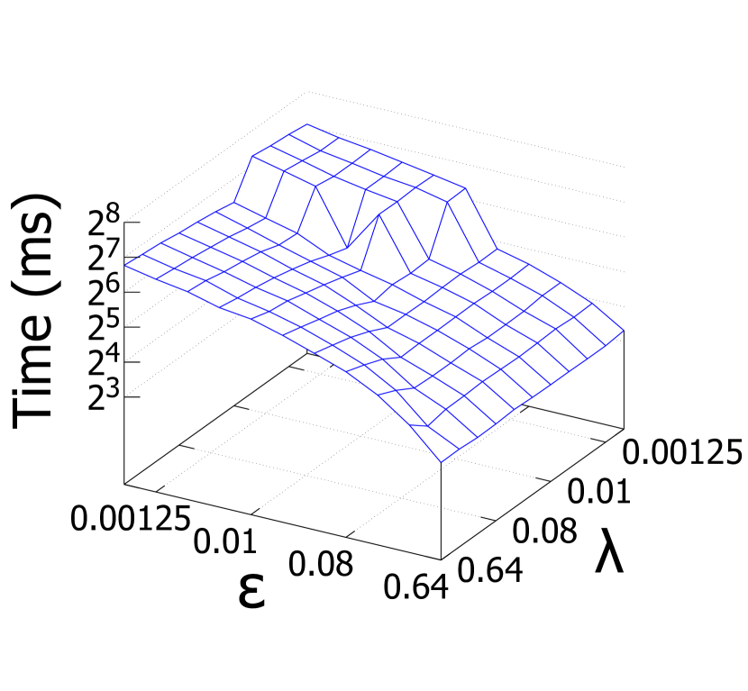
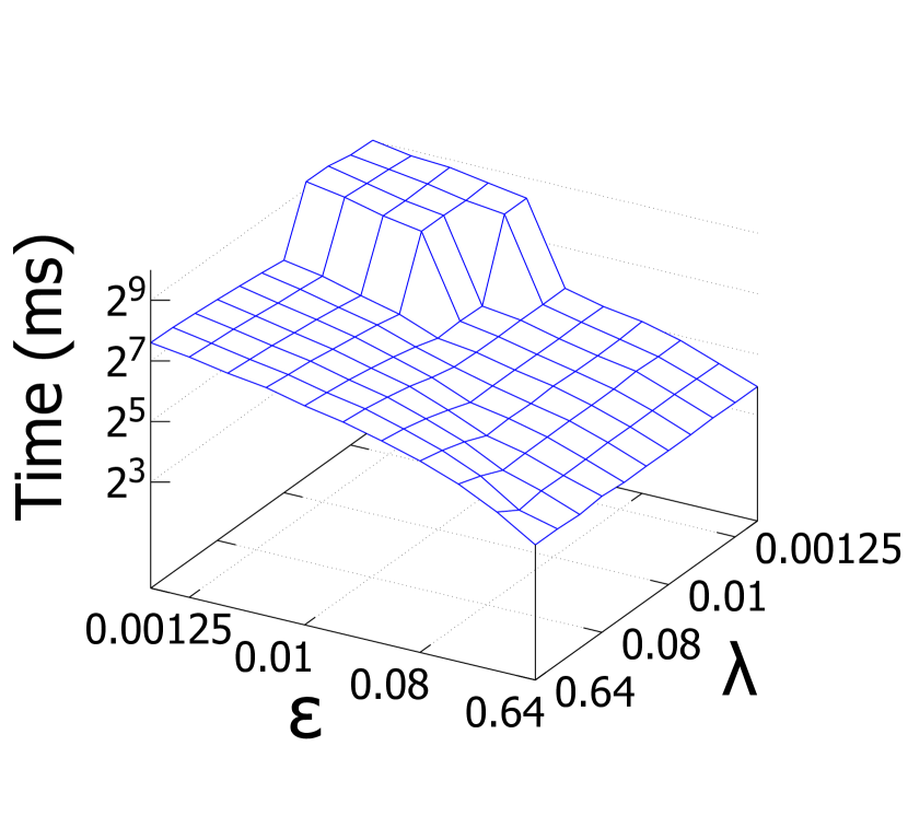
In this section, we provide the additional experimental results on the impact of parameters $\delta$, $\varepsilon$, and $\lambda$ on the performance of our proposed algorithms BiGreedy and BiGreedy+.

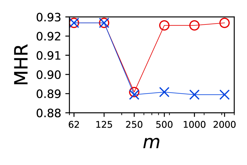
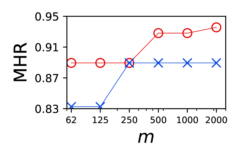
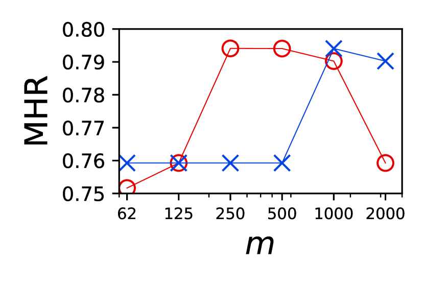
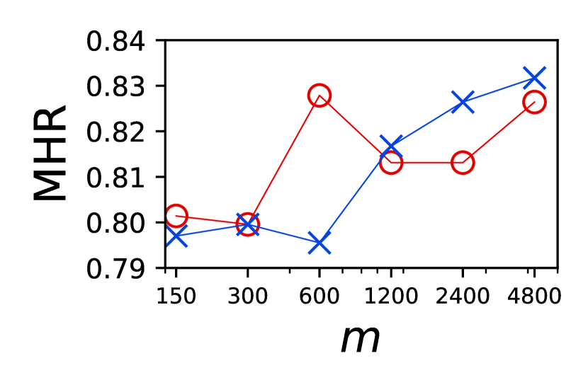
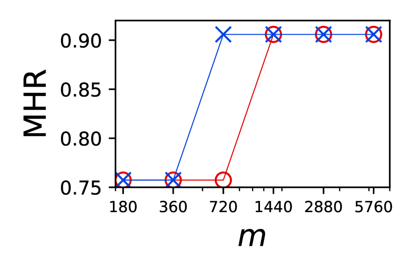
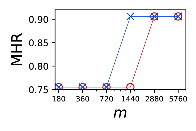
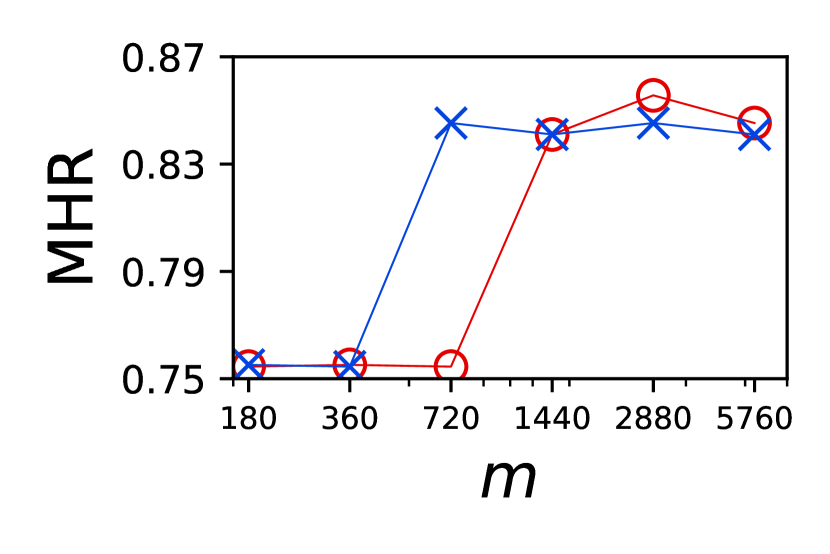
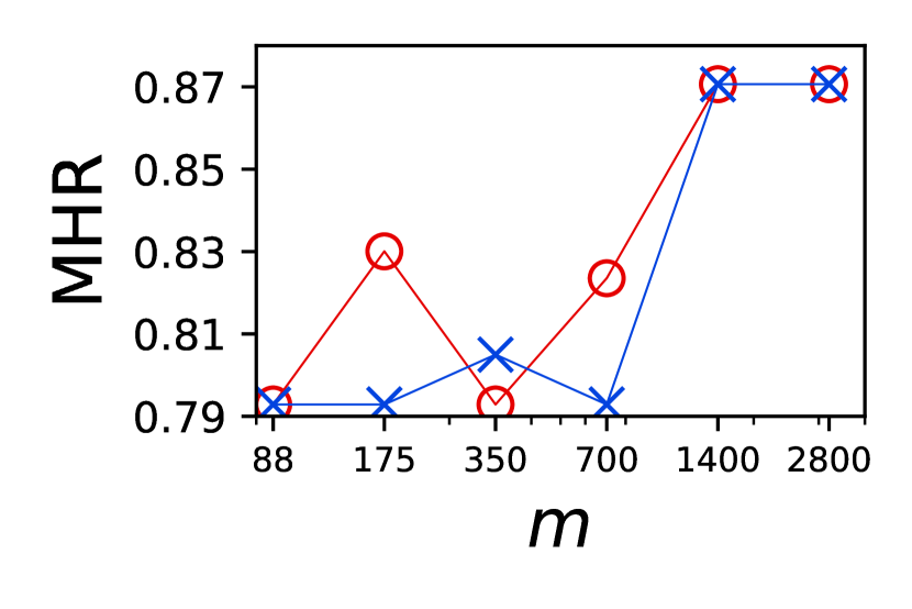
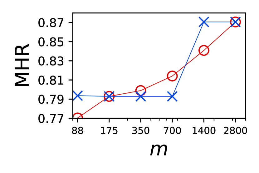
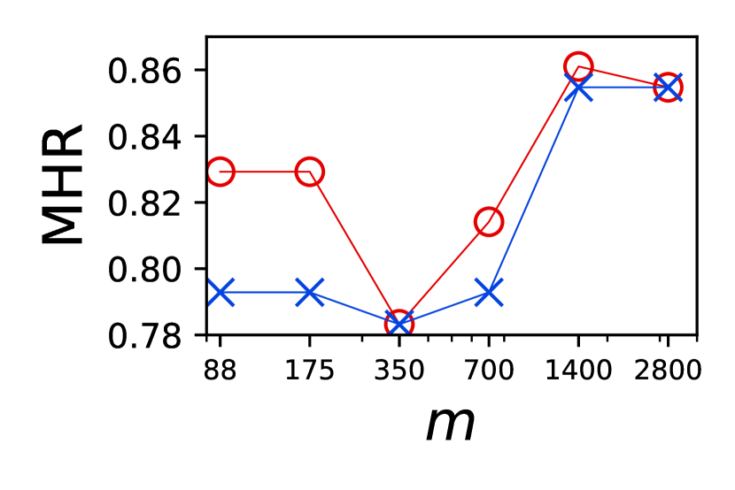
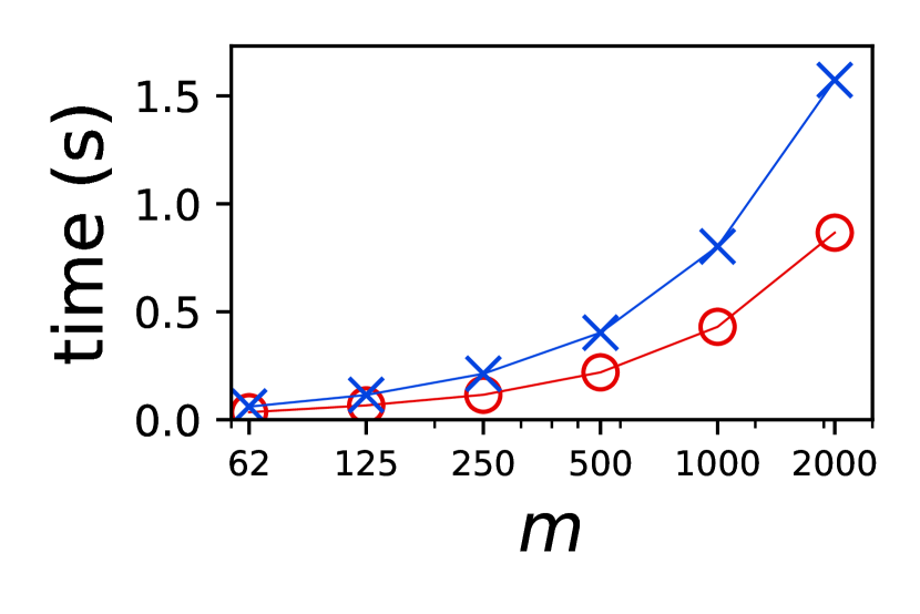
Figures 8(j) and 9(j) present the MHRs and running time of BiGreedy and BiGreedy+ by varying the sample size $m$ of the $\delta$-net in BiGreedy or the maximum sample size $M$ in BiGreedy+. Since the sample size $m$ of a $\delta$-net grows exponentially with respect to $d$ when the value of $\delta$ is fixed, setting a small value of $\delta$ is impractical for high dimensionality $d$. Following existing studies on using $\delta$-nets for RMS problems (Agarwal et al., 2017; Kumar and Sintos, 2018; Wang et al., 2021b), we consider using greater values of $\delta$ for larger $d$’s and testing the corresponding values of $m$ which guarantee that a high-quality solution can be computed in reasonable time. In practice, we use $m=10kd$ for BiGreedy and $M=10kd$ and $m_{0}=0.05M$ for BiGreedy+ by default in the experiments. Here, we further vary $m$ and $M$ in $\{1.25kd,2.5kd,5kd,10kd,20kd,40kd\}$ to show their effects on the performance of BiGreedy and BiGreedy+. First, we observe that the MHRs of both algorithms increase in most cases when the values of $m$ and $M$ grow as the errors in MHR estimations become smaller. However, such a trend does not strictly follow because MRGreedy is an approximation algorithm and might provide worse solutions even when the estimations for MHRs are more accurate. Second, the running time of both algorithms increases nearly linearly with $m$ and $M$. Here, BiGreedy+ runs slower than BiGreedy because the setting of $\lambda$ in this set of experiments ensures that BiGreedy+ reaches $m_{i}\geq M$ for testing whether its solution quality still increases when $M$ is larger. In other experiments, BiGreedy+ runs much faster than BiGreedy as $\lambda=0.04$ is used and BiGreedy+ terminates with smaller $m_{i}$ than $m$. Based on the above results, we find that the MHRs of the solutions of both algorithms hardly increase in most cases when $m,M>10kd$ and thus confirm the default setting of $m=10kd$ in the experiments.

Figures 10(j) and 11(j) present the MHRs and running time of BiGreedy+ for the parameters $\varepsilon\in\{0.00125,0.0025,\ldots,0.64\}$ and $\lambda\in\{0.00125,0.0025,\ldots,0.64\}$. In terms of solution quality, we observe that the MHRs increase significantly when the values of $\varepsilon$ and $\lambda$ decrease from $0.64$ to $0.08$ while becoming steady when the values of $\varepsilon$ and $\lambda$ are smaller. In terms of time efficiency, we find that the decreases of $\varepsilon$ and $\lambda$ both incur higher computational overhead. The trends in both MHRs and running time are attributed to the facts that smaller $\varepsilon$ leads to more $\tau$ values attempted and smaller $\lambda$ causes larger sample sizes before termination. Based on these results, we validate that the parameter settings of $\varepsilon=0.02$ and $\lambda=0.04$ in the experiments lead to reasonable trade-offs between efficiency and effectiveness across different datasets.

References

- (1)
- Agarwal et al. (2004) Pankaj K. Agarwal, Sariel Har-Peled, and Kasturi R. Varadarajan. 2004. Approximating extent measures of points. J. ACM 51, 4 (2004), 606–635.
- Agarwal et al. (2017) Pankaj K. Agarwal, Nirman Kumar, Stavros Sintos, and Subhash Suri. 2017. Efficient Algorithms for k-Regret Minimizing Sets. In SEA. 7:1–7:23.
- Anari et al. (2019) Nima Anari, Nika Haghtalab, Seffi Naor, Sebastian Pokutta, Mohit Singh, and Alfredo Torrico. 2019. Structured Robust Submodular Maximization: Offline and Online Algorithms. In AISTATS. 3128–3137.
- Asudeh et al. (2019a) Abolfazl Asudeh, H. V. Jagadish, Julia Stoyanovich, and Gautam Das. 2019a. Designing Fair Ranking Schemes. In SIGMOD. 1259–1276.
- Asudeh et al. (2017) Abolfazl Asudeh, Azade Nazi, Nan Zhang, and Gautam Das. 2017. Efficient Computation of Regret-ratio Minimizing Set: A Compact Maxima Representative. In SIGMOD. 821–834.
- Asudeh et al. (2019b) Abolfazl Asudeh, Azade Nazi, Nan Zhang, Gautam Das, and H. V. Jagadish. 2019b. RRR: Rank-Regret Representative. In SIGMOD. 263–280.
- Börzsönyi et al. (2001) Stephan Börzsönyi, Donald Kossmann, and Konrad Stocker. 2001. The Skyline Operator. In ICDE. 421–430.
- Cao et al. (2017) Wei Cao, Jian Li, Haitao Wang, Kangning Wang, Ruosong Wang, Raymond Chi-Wing Wong, and Wei Zhan. 2017. k-Regret Minimizing Set: Efficient Algorithms and Hardness. In ICDT. 11:1–11:19.
- Celis et al. (2018a) L. Elisa Celis, Lingxiao Huang, and Nisheeth K. Vishnoi. 2018a. Multiwinner Voting with Fairness Constraints. In IJCAI. 144–151.
- Celis et al. (2018b) L. Elisa Celis, Vijay Keswani, Damian Straszak, Amit Deshpande, Tarun Kathuria, and Nisheeth K. Vishnoi. 2018b. Fair and Diverse DPP-Based Data Summarization. In ICML. 715–724.
- Celis et al. (2018c) L. Elisa Celis, Damian Straszak, and Nisheeth K. Vishnoi. 2018c. Ranking with Fairness Constraints. In ICALP. 28:1–28:15.
- Chester et al. (2014) Sean Chester, Alex Thomo, S. Venkatesh, and Sue Whitesides. 2014. Computing k-Regret Minimizing Sets. Proc. VLDB Endow. 7, 5 (2014), 389–400.
- Chouldechova and Roth (2020) Alexandra Chouldechova and Aaron Roth. 2020. A snapshot of the frontiers of fairness in machine learning. Commun. ACM 63, 5 (2020), 82–89.
- Dong and Zheng (2019) Qi Dong and Jiping Zheng. 2019. Faster Algorithms for k-Regret Minimizing Sets via Monotonicity and Sampling. In CIKM. 2213–2216.
- Faulkner et al. (2015) Taylor Kessler Faulkner, Will Brackenbury, and Ashwin Lall. 2015. k-Regret Queries with Nonlinear Utilities. Proc. VLDB Endow. 8, 13 (2015), 2098–2109.
- Feige (1998) Uriel Feige. 1998. A Threshold of ln n for Approximating Set Cover. J. ACM 45, 4 (1998), 634–652.
- Fisher et al. (1978) M. L. Fisher, G. L. Nemhauser, and L. A. Wolsey. 1978. An analysis of approximations for maximizing submodular set functions—II. In Polyhedral Combinatorics. 73–87.
- Friedman and Nissenbaum (1996) Batya Friedman and Helen Nissenbaum. 1996. Bias in computer systems. ACM Trans. Inf. Sys. 14, 3 (1996), 330–347.
- Fujito (2000) Toshihiro Fujito. 2000. Approximation algorithms for submodular set cover with applications. IEICE Trans. Inf. Syst. 83 (2000), 480–487.
- García-Soriano and Bonchi (2021) David García-Soriano and Francesco Bonchi. 2021. Maxmin-Fair Ranking: Individual Fairness under Group-Fairness Constraints. In KDD. 436–446.
- Halabi et al. (2020) Marwa El Halabi, Slobodan Mitrovic, Ashkan Norouzi-Fard, Jakab Tardos, and Jakub Tarnawski. 2020. Fairness in Streaming Submodular Maximization: Algorithms and Hardness. In NeurIPS. 13609–13622.
- Ilyas et al. (2008) Ihab F. Ilyas, George Beskales, and Mohamed A. Soliman. 2008. A survey of top-k query processing techniques in relational database systems. ACM Comput. Surv. 40, 4 (2008), 11:1–11:58.
- Kleinberg and Tardos (2006) Jon Kleinberg and Éva Tardos. 2006. Algorithm Design. Addison Wesley.
- Kleindessner et al. (2019) Matthäus Kleindessner, Pranjal Awasthi, and Jamie Morgenstern. 2019. Fair k-Center Clustering for Data Summarization. In ICML. 3448–3457.
- Korte and Vygen (2012) Bernhard Korte and Jens Vygen. 2012. Combinatorial Optimization: Theory and Algorithms. Springer Berlin Heidelberg, Berlin, Heidelberg.
- Krause and Golovin (2014) Andreas Krause and Daniel Golovin. 2014. Submodular Function Maximization. In Tractability: Practical Approaches to Hard Problems. Cambridge University Press, 71–104.
- Krause et al. (2008) Andreas Krause, H Brendan McMahan, Carlos Guestrin, and Anupam Gupta. 2008. Robust Submodular Observation Selection. J. Mach. Learn. Res. 9 (2008), 2761–2801.
- Kuhlman and Rundensteiner (2020) Caitlin Kuhlman and Elke A. Rundensteiner. 2020. Rank Aggregation Algorithms for Fair Consensus. Proc. VLDB Endow. 13, 11 (2020), 2706–2719.
- Kumar and Sintos (2018) Nirman Kumar and Stavros Sintos. 2018. Faster Approximation Algorithm for the k-Regret Minimizing Set and Related Problems. In ALENEX. 62–74.
- Luenam et al. (2021) Phoomraphee Luenam, Yau Pun Chen, and Raymond Chi-Wing Wong. 2021. Approximating Happiness Maximizing Set Problems. arXiv:2102.03578 [cs.DB]
- Ma et al. (2022) Hanchao Ma, Sheng Guan, Christopher Toomey, and Yinghui Wu. 2022. Diversified Subgraph Query Generation with Group Fairness. In WSDM. 686–694.
- Mehrotra and Celis (2021) Anay Mehrotra and L. Elisa Celis. 2021. Mitigating Bias in Set Selection with Noisy Protected Attributes. In FAccT. 237–248.
- Moumoulidou et al. (2021) Zafeiria Moumoulidou, Andrew McGregor, and Alexandra Meliou. 2021. Diverse Data Selection under Fairness Constraints. In ICDT. 13:1–13:25.
- Nanongkai et al. (2012) Danupon Nanongkai, Ashwin Lall, Atish Das Sarma, and Kazuhisa Makino. 2012. Interactive regret minimization. In SIGMOD. 109–120.
- Nanongkai et al. (2010) Danupon Nanongkai, Atish Das Sarma, Ashwin Lall, Richard J. Lipton, and Jun (Jim) Xu. 2010. Regret-Minimizing Representative Databases. Proc. VLDB Endow. 3, 1 (2010), 1114–1124.
- Peng and Wong (2014) Peng Peng and Raymond Chi-Wing Wong. 2014. Geometry approach for k-regret query. In ICDE. 772–783.
- Pitoura et al. (2022) Evaggelia Pitoura, Kostas Stefanidis, and Georgia Koutrika. 2022. Fairness in rankings and recommendations: an overview. VLDB J. 31, 3 (2022), 431–458.
- Qi et al. (2018) Jianzhong Qi, Fei Zuo, Hanan Samet, and Jia Cheng Yao. 2018. K-Regret Queries Using Multiplicative Utility Functions. ACM Trans. Database Syst. 43, 2 (2018), 10:1–10:41.
- Qiu et al. (2018) Xianhong Qiu, Jiping Zheng, Qi Dong, and Xingnan Huang. 2018. Speed-Up Algorithms for Happiness-Maximizing Representative Databases. In APWeb/WAIM Workshops. 321–335.
- Saff and Kuijlaars (1997) Edward B. Saff and Amo B. J. Kuijlaars. 1997. Distributing many points on a sphere. Math. Intell. 19, 1 (1997), 5–11.
- Shetiya et al. (2019) Suraj Shetiya, Abolfazl Asudeh, Sadia Ahmed, and Gautam Das. 2019. A Unified Optimization Algorithm For Solving “Regret-Minimizing Representative” Problems. Proc. VLDB Endow. 13, 3 (2019), 239–251.
- Singh and Joachims (2018) Ashudeep Singh and Thorsten Joachims. 2018. Fairness of Exposure in Rankings. In KDD. 2219–2228.
- Soma and Yoshida (2017) Tasuku Soma and Yuichi Yoshida. 2017. Regret Ratio Minimization in Multi-Objective Submodular Function Maximization. In AAAI. 905–911.
- Storandt and Funke (2019) Sabine Storandt and Stefan Funke. 2019. Algorithms for Average Regret Minimization. In AAAI. 1600–1607.
- Stoyanovich et al. (2020) Julia Stoyanovich, Bill Howe, and H. V. Jagadish. 2020. Responsible Data Management. Proc. VLDB Endow. 13, 12 (2020), 3474–3488.
- Stoyanovich et al. (2018) Julia Stoyanovich, Ke Yang, and H. V. Jagadish. 2018. Online Set Selection with Fairness and Diversity Constraints. In EDBT. 241–252.
- Torrico et al. (2021) Alfredo Torrico, Mohit Singh, Sebastian Pokutta, Nika Haghtalab, Joseph (Seffi) Naor, and Nima Anari. 2021. Structured Robust Submodular Maximization: Offline and Online Algorithms. INFORMS J. Comput. 33, 4 (2021), 1590–1607.
- Udwani (2018) Rajan Udwani. 2018. Multi-objective Maximization of Monotone Submodular Functions with Cardinality Constraint. In NeurIPS. 9513–9524.
- Wang et al. (2021a) Yanhao Wang, Francesco Fabbri, and Michael Mathioudakis. 2021a. Fair and Representative Subset Selection from Data Streams. In WWW. 1340–1350.
- Wang et al. (2021b) Yanhao Wang, Yuchen Li, Raymond Chi-Wing Wong, and Kian-Lee Tan. 2021b. A Fully Dynamic Algorithm for k-Regret Minimizing Sets. In ICDE. 1631–1642.
- Wang et al. (2021c) Yanhao Wang, Michael Mathioudakis, Yuchen Li, and Kian-Lee Tan. 2021c. Minimum Coresets for Maxima Representation of Multidimensional Data. In PODS. 138–152.
- Xiao and Li (2022) Xingxing Xiao and Jianzhong Li. 2022. Rank-Regret Minimization. In ICDE. 1848–1860.
- Xie et al. (2019) Min Xie, Raymond Chi-Wing Wong, and Ashwin Lall. 2019. Strongly Truthful Interactive Regret Minimization. In SIGMOD. 281–298.
- Xie et al. (2020a) Min Xie, Raymond Chi-Wing Wong, and Ashwin Lall. 2020a. An experimental survey of regret minimization query and variants: bridging the best worlds between top-k query and skyline query. VLDB J. 29, 1 (2020), 147–175.
- Xie et al. (2018) Min Xie, Raymond Chi-Wing Wong, Jian Li, Cheng Long, and Ashwin Lall. 2018. Efficient k-Regret Query Algorithm with Restriction-free Bound for any Dimensionality. In SIGMOD. 959–974.
- Xie et al. (2020b) Min Xie, Raymond Chi-Wing Wong, Peng Peng, and Vassilis J. Tsotras. 2020b. Being Happy with the Least: Achieving -happiness with Minimum Number of Tuples. In ICDE. 1009–1020.
- Zehlike et al. (2017) Meike Zehlike, Francesco Bonchi, Carlos Castillo, Sara Hajian, Mohamed Megahed, and Ricardo Baeza-Yates. 2017. FA*IR: A Fair Top-k Ranking Algorithm. In CIKM. 1569–1578.
- Zehlike et al. (2021) Meike Zehlike, Ke Yang, and Julia Stoyanovich. 2021. Fairness in Ranking: A Survey. (2021). arXiv:2103.14000 [cs.IR]
- Zeighami and Wong (2019) Sepanta Zeighami and Raymond Chi-Wing Wong. 2019. Finding Average Regret Ratio Minimizing Set in Database. In ICDE. 1722–1725.
- Zheng and Chen (2020) Jiping Zheng and Chen Chen. 2020. Sorting-Based Interactive Regret Minimization. In APWeb/WAIM. 473–490.
- Zheng et al. (2022) Jiping Zheng, Yanhao Wang, Xiaoyang Wang, and Wei Ma. 2022. Continuous k-Regret Minimization Queries: A Dynamic Coreset Approach. IEEE Trans. Knowl. Data Eng. (2022). https://doi.org/10.1109/TKDE.2022.3166835
- Zliobaite (2017) Indre Zliobaite. 2017. Measuring discrimination in algorithmic decision making. Data Min. Knowl. Discov. 31, 4 (2017), 1060–1089.