On the First Law of Thermodynamics in Time-Dependent Open Quantum Systems

Abstract

How to rigorously define thermodynamic quantities such as heat, work, and internal energy in open quantum systems driven far from equilibrium remains a significant open question in quantum thermodynamics. Heat is a quantity whose fundamental definition $d\bar{}\hskip 1.00006ptQ=TdS$ applies only to processes in systems infinitesimally perturbed from equilibrium, and as such, must be accounted for carefully in strongly-driven systems. A key insight from Mesoscopics is that infinitely far from the local driving and coupling of an open quantum system, reservoirs are indeed only infinitesimally perturbed, thereby allowing the heat dissipated to be defined. The resulting partition of the entropy necessitates a Hilbert-space partition of the energetics, leading to an unambiguous operator for the internal energy of an interacting time-dependent open quantum system. Fully general expressions for the heat current and the power delivered by various agents to the system are derived using the formalism of nonequilibrium Green’s functions, establishing an experimentally meaningful and quantum mechanically consistent division of the energy of the system under consideration into Heat flowing out of and Work done on the system. The spatio-temporal distribution of internal energy in a strongly-driven open quantum system is also analyzed. This formalism is applied to analyze the thermodynamic performance of a model quantum machine: a driven two-level quantum system strongly coupled to two metallic reservoirs, which can operate in several configurations–as a chemical pump/engine or a heat pump/engine.

I Introduction

Quantum Thermodynamics has seen substantial progress in recent years in both experimental and theoretical directions [1]. These include but are not limited to quantum thermometry [2, 3, 4, 5, 6, 7, 8, 9, 10, 11, 12], quantum and thermal machines [13, 14, 15, 16, 17], quantum stochastic dynamics [18, 19, 20] and quantum information and computation [21]. Despite these rapid advancements, however, broad consensus on several basic questions of the field has been elusive. The reason for this is not entirely mysterious. The field is, firstly, in relative infancy and, secondly, a melding of two well-established disciplines of physics. A large subset of unresolved questions in quantum thermodynamics thus centers around the need for a careful evaluation of the foundational concepts and laws that the subject builds upon.

One of the key open questions has been the validity and the formulation of the First Law of Thermodynamics for an open quantum system (defined as a quantum system statistically and quantum mechanically open to the environment via some finite coupling) driven far from equilibrium. More concretely, since the First Law is a statement about more than mere energy conservation, we may ask the following: how does one establish an experimentally meaningful and quantum mechanically consistent division of the energy of a far-from-equilibrium quantum system into its Internal Energy, the Work done by the different agents acting and boundary conditions imposed on it, and the Heat flowing from it? An even more basic question that naturally precedes this is whether such a division is even possible given the fundamental uncertainty constraints that quantum mechanics places on the measurement of observables.

These questions have been previously addressed in several works [22, 23, 24, 25, 26, 27, 28, 29], which present highly divergent points of view on the issue. Much of the controversy revolves around how to treat the “Interface” between the system and the environment induced by the System-Reservoir coupling Hamiltonian. An approach based on the ‘Hamiltonian of Mean Force’ concept [22] introduces an ambiguity in the definition of Internal Energy of the system and concludes that it might not even be possible to formulate the First Law, even on a quantum-statistical average level. Another set of analyses [23, 24] proposes dividing up the Coupling Energy between the system and the environment as half of it belonging to the system and half of it belonging to the environment. Others still conclude that the Internal Energy of the nonequilibrium system should be identified by putting the entire Coupling with the System [25, 26, 27] where the last two references specifically employ the Master equation approach and the so-called Mesoscopic leads approach, respectively. A recent study comparing some of these approaches has also emerged [28].

In this work, we shed light on the problem of formulating the First Law of Thermodynamics for a time-dependent open quantum system using insights from Mesoscopic physics [30, 31, 32, 33]. We find that the partitioning of the energetics at the heart of the First Law is dictated by the partitioning of the underlying Hilbert space [34, 35, 36]. This leads naturally to the identification that the Internal Energy operator should be the System Hamiltonian plus half the coupling Hamiltonian.

The systems studied in this work are strongly coupled to their environment and possess broken time-translational symmetry. The mesoscopic modeling of the Hamiltonian governing the nonequilibirum dynamics is done such that the model is both experimentally realistic and computationally tractable while capturing all the relevant physics of the energy and particle flows. Specifically, we start by identifying the conditions under which heat can be unambiguously defined for a strongly-driven system and how one must account for it by carefully considering what role the Reservoirs (which make up the environment) coupled to the system play.

With the proper thermodynamic identifications made, we proceed to derive general expressions for all the different possible forms of energy flows out of the system using the nonequilibrium Green’s functions (NEGF) formalism. The NEGF formalism is a powerful framework for analyzing quantum transport which we utilize to investigate the thermodynamics of a fairly general structure, where the system consists of interacting electronic and phononic degrees of freedom strongly coupled to an environment of non-interacting electrons and phonons. As an application of these formal results, we simulate a strongly driven quantum machine based on Rabi oscillations of a double quantum dot system, investigating in detail its operation as an electrochemical pump and as a heat engine.

This work is organized as follows: In Section II, we give a detailed description of the model time-dependent Hamiltonian that forms the basis of all subsequent derivations and discussions. Section III identifies all the different possible forms of energy flow associated with the system, the role of reservoirs, and Hilbert-space partitioning of physical observables such as energy and entropy. The consequent form of the Internal Energy Operator and the First Law are presented in Sec. IV. In Section V, we derive all the nonequilibrium energy flows and values in terms of the System Green’s functions using the NEGF formalism. In Section VI, we present results and discussion for the simulation of a strongly-driven quantum machine operating as an electrochemical pump and a heat engine, including an analysis of the spatio-temporal evolution of the energy. Finally, the conclusions of our work are presented in Section VII.

II The Time-Dependent Open Quantum System

Figure 1: Schematic representation of a general time-dependent open quantum system [Eq. (1)]. $\mathcal{H_{S}}$ and $\mathcal{H_{R}}$ denote the System and Reservoir (single-particle) Hilbert spaces, respectively, whereas $H_{S}(t)$ and $H_{R}$ describe the System and Reservoir Hamiltoninans, respectively. The Coupling Hamiltonian $H_{SR}$ describes the Interface between the System and the Environment.

A fairly general Hamiltonian for a time-dependent open quantum system (Fig. 1) can be written as

$$H(t)=H_{S}(t)+H_{R}+H_{SR}\,.$$ (1)

The System Hamiltonian $H_{S}(t)$ has explicit time-dependence due to an external drive and is written as the sum of electronic, phononic and electron-phonon coupling terms

$$H_{S}(t)=H_{S,el}(t)+H_{S,ph}(t)+H_{S,el-ph}\,.$$ (2)

The electronic part of the system Hamiltonian $H_{S,el}(t)$ includes electron-electron interactions and has explicit time-dependence from the external electric drive :

$$H_{S,el}(t)=\sum_{n,m}\Bigg{(}[H^{(1)}_{S,el}(t)]_{nm}d^{\dagger}_{n}d_{m}+[H^{(2)}_{S,el}]_{nm}d^{\dagger}_{n}d^{\dagger}_{m}d_{m}d_{n}\Bigg{)},$$ (3)

where $d^{\dagger}_{n}$ $(d_{n})$ creates (removes) an electron in the $n^{th}$ orbital in the system, where $n$ fully specifies both the orbital and the spin degrees of freedom of the electron, and the operators obey fermionic anti-commutation $\{d^{\dagger}_{n},d_{m}\}=\delta_{nm}$. The phononic part $H_{S,ph}(t)$ is given as the sum of a harmonic term and an anharmonic term

$$H_{S,ph}(t)=H_{S,ph}^{hm}(t)+H_{S,ph}^{ahm}\,,$$ (4)

where the time-dependent harmonic part $H_{S,ph}^{hm}(t)$ accounts for an external mechanical drive:

$$H_{S,ph}^{hm}(t)=\sum_{i}\Bigg{(}\frac{P^{\prime 2}_{i}}{2m_{i}}-F^{\prime}_{i}(t)Q^{\prime}_{i}\Bigg{)}+\frac{1}{2}\sum_{i,j}K^{\prime}_{ij}Q^{\prime}_{i}Q^{\prime}_{j}\,,$$ (5)

where $Q^{\prime}_{i}$ and $P^{\prime}_{i}$ are the position and momentum operators, respectively, of the $i^{th}$ atom of the system with mass $m_{i}$, so that we have the canonical quantization condition $[Q^{\prime}_{i},P^{\prime}_{j}]=i\hbar\delta_{ij}$, and also that $P^{\prime}_{i}=m_{i}\dot{Q^{\prime}_{i}}$. The elastic coupling between any two sites $(i,j)$ is given by $K^{\prime}_{ij}$ and the mechanical driving force acting on the $i^{th}$ lattice site is $F^{\prime}_{i}(t)$. Upon rescaling to eliminate $m_{i}$, we get

$$H_{S,ph}^{hm}(t)=\sum_{i}\Bigg{(}\frac{{P}_{i}^{2}}{2}-F_{i}(t)Q_{i}\Bigg{)}+\frac{1}{2}\sum_{i,j}{K}_{ij}Q_{i}Q_{j}\,,$$ (6)

where $P^{\prime}_{i}=\sqrt{m_{i}}P_{i}$, $Q^{\prime}_{i}=\frac{Q_{i}}{\sqrt{m_{i}}}$, $K^{\prime}_{ij}=\frac{{K}_{ij}}{\sqrt{m_{i}m_{j}}}$, and $F^{\prime}_{i}(t)=\sqrt{m_{i}}F_{i}(t)$, so that we now have $P_{i}=\dot{Q_{i}}$ . Finally, upon performing an orthogonal change of basis , we can write the Hamiltonian in diagonal form as

$$H_{S,ph}^{hm}(t)=\sum_{r}\Bigg{(}\frac{P_{r}^{2}}{2}+\frac{\omega_{r}^{2}Q_{r}^{2}}{2}-F_{r}(t)Q_{r}\Bigg{)}\,,$$ (11)

where $P_{r}$ and $Q_{r}$ are momentum and position operators, respectively, of the $r^{th}$ oscillator normal mode in the system, which has frequency $\omega_{r}$, and where we have the quantization condition $[Q_{r},P_{s}]=i\hbar\delta_{rs}$. The anharmonic part $H_{S,ph}^{ahm}$ is given by

$$H_{S,ph}^{ahm}=H_{S,ph}^{(3)}+H_{S,ph}^{(4)}+...\,,$$ (12)

where the cubic term $H_{S,ph}^{(3)}$ can be written as

$$H_{S,ph}^{(3)}=\sum_{p,r,s}[H_{S,ph}^{(3)}]_{prs}Q_{p}Q_{r}Q_{s}\,.$$ (13)

The quartic term $H_{S,ph}^{(4)}$ and all higher-order anharmonic terms can be written analogously. The electron-phonon coupling is

$$H_{S,el-ph}=\sum_{r,n,m}[H_{S,el-ph}]_{rnm}Q_{r}d^{\dagger}_{n}d_{m}+...$$ (14)

and may include higher-order terms in the lattice-electron potential expansion.

The environment is modeled as $M$ perfectly ordered, semi-infinite Reservoirs of non-interacting electrons and phonons, each at Temperature $T_{\alpha}$ and chemical potential $\mu_{\alpha}$, with the Hamiltonian

$$H_{R}=H_{R,el}+H_{R,ph}$$ (15)

where the electronic sector of the $\alpha^{th}$ reservoir is

$$H_{R,el,\alpha}=\sum_{k\in\alpha}\epsilon_{k}c_{k}^{\dagger}c_{k},$$ (16)

where $c_{k}^{\dagger}$ $(c_{k})$ creates (removes) an electron in eigenmode $k$ in the reservoir and obey $\{c_{k}^{\dagger},c_{l}\}=\delta_{kl}$, and we have $\sum_{\alpha=1}^{M}H_{R,el,\alpha}=H_{R,el}$. The phononic sector of the $\alpha^{th}$ reservoir is given by the Hamiltonian

$$H_{R,ph,\alpha}=\sum_{q\in\alpha}\Bigg{(}\frac{P_{q}^{2}}{2}+\frac{\omega_{q}^{2}U_{q}^{2}}{2}\Bigg{)}\,,$$ (17)

where $P_{q}$ and $U_{q}$ are momentum and position operators, respectively, for the $q^{th}$ oscillator normal mode with frequency $\omega_{q}$ in the reservoir, satifying the canonical quantization condition $[U_{p},P_{q}]=i\hbar\delta_{pq}$. Finally, we have $\sum_{\alpha=1}^{M}H_{R,ph,\alpha}=H_{R,ph}$.

The coupling between the System and the Reservoirs is given by the Coupling Hamiltonian

$$H_{SR}=H_{SR,el}+H_{SR,ph}\,,$$ (18)

where the electronic coupling to the $\alpha^{th}$ reservoir is given by

$$H_{SR,el,\alpha}=\sum_{k\in\alpha,n}(V_{kn}^{el}c_{k}^{\dagger}d_{n}+h.c.),$$ (19)

with $H_{SR,el}=\sum_{\alpha=1}^{M}H_{SR,el,\alpha}$, and the phononic coupling to the $\alpha^{th}$ reservoir is given by

$$H_{SR,ph,\alpha}=\frac{1}{2}\sum_{q\in\alpha,r}\left(V_{qr}^{ph}U_{q}Q_{r}+V_{rq}^{ph}Q_{r}U_{q}\right),$$ (20)

with $V_{rq}^{ph}=V_{qr}^{ph}$ and $H_{SR,ph}=\sum_{\alpha=1}^{M}H_{SR,ph,\alpha}$.

II.1 Physical basis of the model Hamiltonian

We note some points here about the modeling of the Hamiltonian just presented that are important from both physical and computational points of view.

First, the Reservoirs are modeled as non-interacting, semi-infinite, and perfectly ordered so that they faithfully represent the external macroscopic circuit used to impose any nonequilibrium bias on the system and to measure the resultant flows of charge and energy. As counters of charge and energy flowing out the system, it makes little sense to include two-body interactions in the Reservoirs, since that would significantly complicate the task of calculating these quantities, and many-body correlations are not relevant in such a macroscopic electric/thermal circuit in any case. The interesting case of superconducting Reservoirs [39, 40, 41, 42] is outside the scope of the analysis in this article.

The coupling between the System and the Reservoir $H_{SR}$ is also taken to be quadratic. Realistically, this is because the electrons in the metallic Reservoirs, modeled by $H_{R}$, are well screened and hence any interaction between the electrons in the System and the Reservoir can be treated with the method of image charges [43], the screening charges in the Reservoirs treated as slave degrees of freedom, rather than as independent quantum modes. This is justified because the screening charges in the reservoirs respond at the plasma frequency, which is much greater than typical response frequencies of a mesosopic system. Moreover, if many-body effects in the interfacial regions of the reservoirs are important, these regions can simply be included in the System.

Second, the number of Reservoir degrees of freedom entering $H_{SR}$ is a set of measure zero [44, 45] compared to the full (infinite) Reservoir Hilbert space, with only a few frontier orbitals taking part in coupling the environment to the System. This is because tunnel coupling is local at the Interface between the System and Reservoir and the screening charges are also localized at the Interface . The same holds true for the phononic degrees of freedom, whose elastic coupling is short-ranged [48]. A model calculation of the spatio-temporal dynamics of the Interface, illustrating these principles, is presented in Secs. VI.2.1 and VI.3.1.

III Non-Equilibrium Thermodynamic Quantities

With the open quantum system defined, we now compute the nonequilibrium thermodynamic quantities of the system.

III.1 Work done by external forces

Following the so-called Inclusive definition of work, standard in the Quantum Thermodynamics literature [49] (in contrast with the Exclusive definition [50]), we identify the time rate of change of the expectation value of the total Hamiltonian as the rate of work done by external forces, $\dot{W}_{ext}(t)$, which for the form assumed for the Hamiltonian, we can compute as

$$\frac{d}{dt}\langle H(t)\rangle\equiv\dot{W}_{ext}(t)\ =\langle\dot{H}_{S}(t)\rangle\,,$$ (21)

where $\langle\,\rangle$ denotes the quantum and statistical average.

The equality can be proved [51] by noting that $\langle H(t)\rangle=\mathrm{Tr}\{\rho(t)H(t)\}$, with $\rho(t)$ denoting the full density matrix at time $t$ and $\mathrm{Tr}\{\}$ denoting the Trace operation over the full Fock Space, and using the chain rule we can write

$$\frac{d}{dt}\langle H(t)\rangle=\mathrm{Tr}\{\dot{\rho}(t)H(t)+\rho(t)\dot{H}(t)\}\,,$$ (22)

which, with the equation of motion of the density matrix

$$i\hbar\dot{\rho}=[H(t),\rho(t)]\,,$$ (23)

and cyclicity of the Trace gives the stated result, $\dot{W}_{ext}(t)\ =\langle\dot{H}_{S}(t)\rangle$, since the time-dependence is only in the System Hamiltonian $H_{S}(t)$.

Furthermore, since the time-dependence in $H_{S}(t)$ sits only in the one-body terms, we get

$$\dot{W}_{ext}(t)=\dot{W}_{ext,el}(t)+\dot{W}_{ext,ph}(t)\,,$$ (24)

where the power delivered by the electronic drive is

$$\dot{W}_{ext,el}(t)=\sum_{n,m}\langle[\dot{H}^{(1)}_{S,el}(t)]_{nm}d^{\dagger}_{n}d_{m}\rangle\,,$$ (25)

and that by the mechanical drive is

$$\dot{W}_{ext,ph}(t)=-\sum_{r}\dot{F}_{r}(t)\langle Q_{r}\rangle$$ (26)

III.2 Particle Current and Electrochemical Power

The electronic particle current $I_{\alpha,el}^{N}(t)$ into reservoir $\alpha$ is given by the rate of change of the expectation value of the occupation number operator $N_{\alpha}=\sum_{k\in\alpha}c_{k}^{\dagger}c_{k}$ of the $\alpha^{th}$ reservoir

$$I_{\alpha,el}^{N}(t):=\frac{d}{dt}\langle N_{\alpha}\rangle\,,$$ (27)

which can be evaluated as

$$\frac{d}{dt}\langle N_{\alpha}\rangle=\frac{-i}{\hbar}\langle[N_{\alpha},H(t)]\rangle=\frac{-i}{\hbar}\langle[N_{\alpha},H_{SR}]\rangle\,.$$ (28)

Using the identities $[A,BC]=\{A,B\}C-B\{C,A\}=[A,B]C-B[C,A]$, we obtain the particle current as

$$I_{\alpha,el}^{N}(t)=\frac{-i}{\hbar}\sum_{k\in\alpha,n}[V_{kn}^{el}\langle c_{k}^{\dagger}d_{n}\rangle-(V^{el}_{kn})^{*}\langle d_{n}^{\dagger}c_{k}\rangle]\,.$$ (29)

The electrical current is obtained by multiplying the above equation by the electric charge quantum.

The electrochemical power delivered to reservoir $\alpha$ is $\mu_{\alpha}I^{N}_{\alpha,el}(t)$ and the net electrochemical power delivered to the system by the reservoirs is

$$\dot{W}_{elec}(t):=\sum_{\alpha}-\mu_{\alpha}I_{\alpha,el}^{N}(t).$$ (30)

III.3 Heat, the Role of Reservoirs, and Hilbert space partition

Heat is a quantity whose fundamental definition $d\bar{}\hskip 1.00006ptQ=TdS$ is only valid for quasi-static processes [52, 53], and as such, must be accounted for carefully in strongly-driven systems. This requirement is met exactly by the non-interacting semi-infinite reservoirs to which the nonequilibrium system is coupled. The relevant properties of the reservoir model have been long established in the Mesoscopics and Quantum Transport literature [54, 55, 56], where they enforce an Ordering of Limits such that one must take the limit of the Reservoir size going to infinity $L\to\infty$ before taking limit of the adiabatic perturbation switch-on time going to infinity $t_{adiab}\to\infty$. Physically, $t_{adiab}$ is related to the timescale of setting up and carrying out the experiment. This order of limits ensures that any electrons or phonons emitted by the System into the Reservoirs cannot be coherently backscattered into the system (causing decoherence of any quanta emitted into the Reservoirs despite the absence of 2-body interactions) and that the distributions of charge and energy in the Reservoirs cannot be depleted due to flows mediated by the System.

The entropy is given by the von Neumann formula [57]

$$S=-{\rm Tr}\{\rho\ln\rho\},$$ (31)

where $\rho$ is the density matrix of the universe and we have set $k_{B}=1$. For small deviations from an initial density matrix $\rho_{0}$, the linear change in entropy is

$$dS=-{\rm Tr}\{d\rho\ln\rho_{0}\}$$ (32)

(See Appendix A for a derivation.) For an initial equilibrium state, $\rho_{0}$ is given by the grand canonical ensemble

$$\rho_{0}=\frac{e^{-\beta(H-\mu N)}}{\cal Z},$$ (33)

where ${\cal Z}={\rm Tr}\{e^{-\beta(H-\mu N)}\}$ is the grand partition function, leading to the standard result

$$TdS={\rm Tr}\{d\rho(H-\mu N)\}.$$ (34)

In order to see how the heat $TdS$ is partitioned among the various subsystems, it is useful to first consider the case of independent fermions. Then $TdS=\sum_{\gamma}TdS_{\gamma}$, where the heat added to subsystem $\gamma$ is [34, 35]

$$TdS_{\gamma}=\int d\varepsilon\,\mathbb{Tr}^{(1)}_{\gamma}\{A(\varepsilon)\}(\varepsilon-\mu)df(\varepsilon),$$ (35)

where $A(\varepsilon)=\delta(\varepsilon-h^{(1)})$ is the spectral function, with $h^{(1)}$ the Hilbert-space operator corresponding to the Fock-space Hamiltonian $H^{(1)}$, and $df(\varepsilon)=f(\varepsilon)-f_{0}(\varepsilon)$ is the linear deviation of the distribution function from the initial equilibrium Fermi-Dirac distribution. Here $\mathbb{Tr}^{(1)}_{\gamma}$ is the trace over the subspace $\gamma$ of the single-particle Hilbert-space. We note that $\gamma\in\{S,R\}$ where $S$ denotes the subspace/subsystem containing all the degrees of freedom belonging to the system and $R=\cup_{\alpha=1}^{M}R_{\alpha}$, where $R_{\alpha}$ denotes the subspace/subsystem containing all the degrees of freedom belonging to the $\alpha^{th}$ reservoir. Specifically,

$$\mathbb{Tr}^{(1)}_{\gamma}\{O^{(1)}\}=\mathbb{Tr}^{(1)}\{\Pi_{\gamma}\,O^{(1)}\},$$ (36)

where

$$\Pi_{\gamma}=\sum_{x\in\gamma}|x\rangle\langle x|$$ (37)

is the projection operator onto subspace $\gamma$ of the single-particle Hilbert space and $O^{(1)}$ is any linear operator on the single-particle Hilbert space.

Eq. (35) may be integrated to obtain the equilibrium subsystem entropy

$$S_{\gamma}=\int d\varepsilon\,\mathbb{Tr}^{(1)}_{\gamma}\{A(\varepsilon)\}s(\varepsilon),$$ (38)

which is non-singular [34] and respects the Third Law of Thermodynamics as $T\rightarrow 0$, where

$$s(\varepsilon)=\beta(\varepsilon-\mu)f(\varepsilon)+\ln(1+e^{-\beta(\varepsilon-\mu)}).$$ (39)

The connection of the entropy partition given by Eq. (35) and the required energetic partition is determined by the identity $\varepsilon A(\varepsilon)=h^{(1)}A(\varepsilon)$, which allows Eq. (35) to be rewritten as

$$TdS_{\gamma}=d\langle\left.H^{(1)}\right|_{\gamma}\rangle-\langle\left.dH^{(1)}\right|_{\gamma}\rangle-\mu d\langle N_{\gamma}\rangle,$$ (40)

where $\left.H^{(1)}\right|_{\gamma}$ is the Fock-space operator corresponding to the partition of $h^{(1)}$ onto subspace $\gamma$ [36]

$$\left.h^{(1)}\right|_{\gamma}\equiv\frac{1}{2}\{h^{(1)},\Pi_{\gamma}\},$$ (41)

where $\{A,B\}=AB+BA$ is the anticommutator. (See Appendix A for details of the derivation.) The symmetrization in the definition (41) is needed to ensure the hermiticity of the observable $\left.H^{(1)}\right|_{\gamma}$, which satisfies

$$H^{(1)}=\sum_{\gamma}\left.H^{(1)}\right|_{\gamma}.$$ (42)

We point out that any energetic partition other than that dictated by Hilbert space partitioning as given by Eq. (41) will lead to a singular entropy partition [36] and a violation of the Third Law, because only the Hilbert space partition described above allows for the detailed cancellation of the separately divergent terms in Eq. (39) as $\beta\rightarrow\infty$. The singular character of the entropy for alternate energetic partitions was pointed out previously by Esposito et al. [58].

The partition of the full Hamiltonian onto reservoir $\alpha$ is

$$\left.H\right|_{\gamma=R_{\alpha}}=H_{R,\alpha}+\frac{1}{2}H_{SR,\alpha},$$ (43)

where $H_{R,\alpha}$ is diagonal on the partition, while $H_{SR,\alpha}$ is purely off-diagonal, and thus acquires a factor of 1/2 via Eq. (41). The partition goes through as in the independent-particle case (41) because $H^{(2)}$ is system diagonal (see Appendix A for details). The same holds true for phonon anharmonic terms and electron-phonon interactions, both of which vanish within the reservoirs, so that Eq. (43) is valid for the full Hamiltonian.

III.4 Heat current

We now compute the heat current into reservoir $\alpha$ by extending the thermodynamic identity (40) to the time-dependent nonequilibrium regime, where the chemical potentials and temperatures of the various reservoirs can differ by arbitrarily large amounts, but where it is assumed that the separate equilibrium distributions in the macroscopic reservoirs are perturbed only linearly from their respective equilibrium states due to energy and particle flows mediated by the system:

$$I_{\alpha}^{Q}(t)\equiv T_{\alpha}\frac{d}{dt}S_{\alpha}=\frac{d}{dt}\langle\left.H\right|_{\gamma=R_{\alpha}}\rangle-\langle\left.\dot{H}\right|_{\gamma=R_{\alpha}}\rangle-\mu_{\alpha}\frac{d}{dt}\langle N_{\alpha}\rangle\,,$$ (44)

where, to lighten notation, we write $N_{\alpha}\equiv N_{\gamma=R_{\alpha}}$, which denotes the particle number operator for reservoir $\alpha$. We remark that the interpretation of Eq. (44) as a bona fide heat current is valid for arbitrary nonequilibrium steady-state [59] and slowly-varying flows, but that rapidly-varying transient flows described by Eq. (44) may simply be identified as one component of the total energy flux.

We next specialize to the case where $H_{R}$ and $H_{SR}$ are independent of time. (For an analysis of the general time-dependent case, see Appendix LABEL:full_tdpt_generalize_app.) It is convenient to write the heat current as the sum of two terms

$$I_{\alpha}^{Q}(t)=I_{\alpha}^{Q,conv}(t)+I_{\alpha}^{Q,tr}(t)\,,$$ (45)

where

$$I_{\alpha}^{Q,conv}(t)=\frac{d}{dt}\langle H_{R,\alpha}\rangle-\mu_{\alpha}\frac{d}{dt}\langle N_{\alpha}\rangle$$ (46)

is the conventional component of the heat current and reduces to the Bergfield-Stafford formula [60] in steady state, and

$$I_{\alpha}^{Q,tr}(t)=\frac{1}{2}\frac{d}{dt}\langle H_{SR,\alpha}\rangle\,.$$ (47)

is the transient component of the heat current which vanishes in steady state. We further define the heat currents for the electronic and phononic sectors separately by writing

$$I_{\alpha,el/ph}^{Q}(t)=I_{\alpha,el/ph}^{Q,conv}(t)+I_{\alpha,el/ph}^{Q,tr}(t)\,,$$ (48)

where

$$I_{\alpha,el/ph}^{Q,conv}(t)=\frac{d}{dt}\langle H_{R,el/ph,\alpha}\rangle-\mu_{\alpha}\frac{d}{dt}\langle N_{\alpha}\rangle\,,$$ (49)

with $\mu_{\alpha}=0$ $\forall\alpha$ for phonons, and

$$I_{\alpha,el/ph}^{Q,tr}(t)=\frac{1}{2}\frac{d}{dt}\langle H_{SR,el/ph,\alpha}\rangle\,.$$ (50)

Carrying out commutator evaluations similar to that for the particle current, we get the conventional component of electronic heat current [60]

$$I_{\alpha,el}^{Q,conv}(t)=\frac{-i}{\hbar}\sum_{k\in\alpha,n}(\epsilon_{k}-\mu_{\alpha})[V_{kn}^{el}\langle c_{k}^{\dagger}d_{n}\rangle-(V_{kn}^{el})^{*}\langle d_{n}^{\dagger}c_{k}\rangle]\,,$$ (51)

which can be cast in terms of an energy weighted particle current (for the $k^{th}$ mode) as

$$I_{\alpha,el}^{Q,conv}(t)=\sum_{k\in\alpha,n}(\epsilon_{k}-\mu_{\alpha})I_{k}^{N}(t)\,,$$ (52)

where $I_{k}^{N}(t)=\frac{-i}{\hbar}[V_{kn}^{el}\langle c_{k}^{\dagger}d_{n}\rangle-(V^{el}_{kn})^{*}\langle d_{n}^{\dagger}c_{k}\rangle]$. The transient component of the electronic heat current $I_{\alpha,el}^{Q,tr}(t)$ can be computed by the taking the time-derivative of

$$\frac{1}{2}\langle H_{SR,el,\alpha}\rangle=\frac{1}{2}\sum_{k\in\alpha,n}\langle V_{kn}^{el}c_{k}^{\dagger}d_{n}+h.c.\rangle$$ (53)

The conventional component of the phononic heat current [61, 62, 63] can be analogously evaluated as

$$I_{\alpha,ph}^{Q,conv}(t)=-\sum_{q\in\alpha,r}V^{ph}_{qr}\langle P_{q}Q_{r}\rangle\,,$$ (54)

and the transient component of the phononic heat current $I_{\alpha,ph}^{Q,tr}(t)$ can be computed by taking the time-derivative of

$$\frac{1}{2}\langle H_{SR,ph,\alpha}\rangle=\frac{1}{2}\sum_{q\in\alpha,r}V_{qr}^{ph}\langle U_{q}Q_{r}\rangle\,.$$ (55)

The time derivative of the expectation value of the full Hamiltonian partitioned onto the Reservoir subspace $\left.H\right|_{\gamma=R}$ has a simple interpretation: it is the total energy current flowing into the Reservoirs $\sum_{\alpha}I_{\alpha}^{E}(t)$ i.e.

$$\frac{d}{dt}\langle H_{R}(t)+\frac{1}{2}H_{SR}\rangle=\sum_{\alpha}I_{\alpha}^{E}(t)\,.$$ (56)

At infinity, this in turn is just the electrical (or electrochemical) power delivered to the reservoir plus the heat current flowing into it

$$\sum_{\alpha}I_{\alpha}^{E}(t)=\sum_{\alpha}\mu_{\alpha}I_{\alpha,el}^{N}(t)+\sum_{\alpha}I_{\alpha}^{Q}(t)\,,$$ (57)

where $I_{\alpha}^{Q}(t)=I_{\alpha,el}^{Q}(t)+I_{\alpha,ph}^{Q}(t)$. We note that while the electrochemical power and electronic heat current at infinity can be properly interpreted as such for general nonequilibrium driving of the system, according to the arguments given above, the phonon contribution to Eq. (57) may only be identified as a bona fide contribution to the heat current for steady-state or slowly varying flows, and may simply be a contribution to the total energy flux into the reservoirs for rapid transient flows.

IV The First Law of Quantum Thermodynamics

From the discussion in Sec. III.1, specifically Eq. (21), it follows that

$$\frac{d}{dt}\langle H_{S}(t)+H_{SR}+H_{R}\rangle=\dot{W}_{ext}(t)\,.$$ (58)

Furthermore, with the identification of Sec. III.3, specifically Eq. (57), we get

$$\frac{d}{dt}\langle H_{S}(t)+\frac{1}{2}H_{SR}\rangle = \dot{W}_{ext}(t)+(\sum_{\alpha}-\mu_{\alpha}I_{\alpha}^{N}(t))+$$ (59)

$$(\sum_{\alpha}-I_{\alpha}^{Q}(t))\,.$$

It is then clear that the internal energy operator for the “System” must be recognized as sum of the System Hamiltonian and half the Coupling Hamiltonian. Defining $\dot{W}_{elec}(t):=\sum_{\alpha}-\mu_{\alpha}I_{\alpha,el}^{N}(t)$ as the electrochemical power delivered to the system and $\dot{Q}(t):=\sum_{\alpha}-I_{\alpha}^{Q}(t)$ as the heat current flowing into the system allows us to write the First Law of Quantum Thermodynamics as lcr ddt⟨U_sys(t) ⟩= ˙W_ext(t)+˙W_elec(t) + ˙Q(t)  , where the Internal Energy operator $U_{sys}(t)$ for the open quantum system is just the Hamiltonian partitioned on the system Hilbert space

$$U_{sys}(t)\equiv\left.H(t)\right|_{S}=H_{S}(t)+\frac{1}{2}H_{SR}\,.$$ (60)

This analysis lays to rest any ambiguity about the internal energy operator and gives a quantum mechanically consistent and experimentally meaningful division of the energetics of a fairly general open quantum system. We also note that this identification of the First Law and Internal Energy operator holds true even in the more general case where both the coupling and reservoirs become explicitly time-dependent, as discussed in Appendix LABEL:full_tdpt_generalize_app.

The definition (60) agrees with that proposed by Ludovico et al. [23] for the specific model of a single sinusoidally driven Fermionic resonant level coupled to a single reservoir (supported in the subsequent work of Bruch et al. [24]), as well as with that put forward by Stafford and Shastry [64, 34, 35] for an independent Fermion system in steady state, but disagrees with those put forward by Esposito et al. [25], Strasberg and Winter [26], and Lacerda et al. [27].

While Eq. (60) provides an explicit quantum mechanical operator for the internal energy, it should be noted that the other thermodynamic quantities entering the First Law cannot in general be associated with explicit quantum operators. Work, being a path (and not a state) function cannot, in general, be a Quantum Operator [66, 67]. Furthermore, Heat (again a path function) also cannot have a quantum operator associated with it since it is a statistical quantity ($d\bar{}\hskip 1.00006ptQ=TdS$) defined unambiguously only under the special conditions discussed in Sec. III.3.

IV.1 Energy Density

To further study the spatio-temporal distribution of energy in the driven open quantum system—for the special case where 2-body interactions are absent—we make use of a general result for the spatial density of any one-body observable [36, 68]. The energy density is given by

$$\rho_{H}(x,t)=\mbox{Tr}\left\{\rho(t)\left.H^{(1)}\right|_{x}(t)\right\},$$ (61)

where $\left.H^{(1)}\right|_{x}(t)$ is the Fock-space operator corresponding to the Hilbert-space Hamiltonian density

$$\left.h^{(1)}\right|_{x}(t)=\frac{1}{2}\{h^{(1)}(t),|x\rangle\langle x|\}.$$ (62)

V Evaluating the Time-Dependent Energetics: NEGF Formulas

We employ the Nonequilibrium Green’s function (NEGF) formalism [69, 70, 71, 30, 31] to evaluate all the terms appearing in the First Law (IV), each term on the LHS of which we have evaluated in terms of the expectation values in Eqs. (24), (29), (52), and (54), and the time derivatives of Eqs. (53) and (55). Here we present only the final results of our analysis and defer the relevant details of the derivations and methods of evaluation to Appendix B. We also note that the NEGF formalism has a well-established connection with the S-Matrix formalism [72]—another technique often employed in quantum transport and thermodynamics. A key advantage of NEGF is its simplicity and power in computing one-body (or even few-body) observables. This is in contrast to the Master equation approach [73, 32, 30], which works in the full many-particle Hilbert space.

V.1 Internal energy

The expectation value of the internal energy operator defined in Eq. (60) can be evaluated in terms of the system Green’s functions. The first term in $U_{sys}(t)$ can be written as a sum of three terms

$$\langle H_{S}(t)\rangle=\langle H_{S,el}(t)\rangle+\langle H_{S,ph}(t)\rangle+\langle H_{S,el-ph}\rangle\,,$$ (63)

where the electronic part can be written as

$$\langle H_{S,el}(t)\rangle = -i\mathbb{Tr}^{(1)}\Bigg{\{}H^{(1)}_{S,el}(t)G^{<}(t,t)\Bigg{\}}$$ (64)

$$-i\mathbb{Tr}^{(2)}\Bigg{\{}H^{(2)}_{S,el}G^{(2)}(t,t)\Bigg{\}}\,,$$

where the system electronic Lesser Green’s function is defined as

$$G^{<}_{nm}(t,t_{1})=i\langle d_{m}^{\dagger}(t_{1})d_{n}(t)\rangle\,,$$ (65)

and the 2-body electronic Green’s function is defined as

$$G^{(2)}_{nnmm}(t,t)=i\langle d^{\dagger}_{n}(t)d^{\dagger}_{m}(t)d_{m}(t)d_{n}(t)\rangle$$ (66)

(see Appendix B for the method of their evaluation). The phononic part can be written as

$$\langle H_{S,ph}(t)\rangle = \frac{i}{2}\mathbb{Tr}^{(1)}\Bigg{\{}\Bigg{(}\frac{\partial^{2}}{\partial t\partial t^{\prime}}+K\Bigg{)}\left.D^{<}(t,t^{\prime})\right|_{t=t^{\prime}}\Bigg{\}}$$ (67)

$$+\frac{1}{\hbar}\int_{-\infty}^{t}\,dt^{\prime}\Bigg{[}\mathbf{F}(t)\mathcal{D}(t,t^{\prime})\mathbf{F}^{\mathrm{T}}(t^{\prime})\Bigg{]}$$

$$-i\mathbb{Tr}^{(3)}\Bigg{\{}H_{S,ph}^{(3)}D^{ahm}(t,t,t)\Bigg{\}}\,,$$

where $K$ denotes a matrix whose elements $K_{ij}$ are the harmonic couplings introduced in Eq. (6), and $\mathbf{F}(t)=(...,F_{r}(t),...)$, is a (row) vector whose elements are the mechanical driving forces acting on the system. The system phononic Lesser Green’s function is

$$D^{<}_{rs}(t,t_{1})=-i\langle Q_{s}(t_{1})Q_{r}(t)\rangle$$ (68)

and $\mathcal{D}(t,t^{\prime})$ is the time-ordered phonon Green’s function, to be evaluated in the absence of the time-dependent mechanical drive, whose matrix element is defined as

$$\mathcal{D}_{rs}(t,t^{\prime})=-i\langle\mathrm{T}(Q_{r}(t)Q_{s}(t^{\prime}))\rangle\,,$$ (69)

where $\mathrm{T}$ denotes the time-ordering operator. Finally, $D^{ahm}_{prs}(t,t,t)=i\langle Q_{p}(t)Q_{r}(t)Q_{s}(t)\rangle$ is the lowest-order anharmonic phonon Green’s function (higher-order phononic Green’s functions can be constructed analogously). The electron-phonon coupling contribution is

$$\langle H_{S,el-ph}\rangle=-i\mathbb{Tr}^{(2)}\Bigg{\{}H_{S,el-ph}G^{el-ph}(t,t,t)\Bigg{\}}\,,$$ (70)

where the electron-phonon Green’s function is defined as $G^{el-ph}_{rnm}(t,t,t)=i\langle Q_{r}(t)d^{\dagger}_{n}(t)d_{m}(t)\rangle$.

The second term in the internal energy may be evaluated as (see Appendix B for details)

$$\langle H_{SR}\rangle=\sum_{\alpha=1}^{M}\Bigg{(}\langle H_{SR,el,\alpha}(t)\rangle+\langle H_{SR,ph,\alpha}(t)\rangle\Bigg{)},$$ (71)

where the electronic part is given by

$$\langle H_{SR,el,\alpha}(t)\rangle = 2\int_{-\infty}^{+\infty}\,\frac{d\omega}{2\pi}\int_{-\infty}^{+\infty}\,dt_{1}\mathbb{ImTr}^{(1)}\Bigg{\{}e^{-i\omega(t_{1}-t)}$$

$$[G^{<}(t,t_{1})\Sigma^{A}_{\alpha}(\omega)+G^{R}(t,t_{1})\Sigma^{<}_{\alpha}(\omega)]\Bigg{\}}\,,$$

where the system electronic Retarded Green’s function is defined as

$$G^{R}_{nm}(t,t_{1})=-i\theta(t-t_{1})\langle\{d_{n}(t),d_{m}^{\dagger}(t_{1})\}\rangle\,,$$ (73)

and $\Sigma^{A}(\omega)$ and $\Sigma^{<}(\omega)$ are the advanced and lesser electronic self-energy functions, respectively, given by

$$[\Sigma^{A/<}_{\alpha}(\omega)]_{nm}=\sum_{k\in\alpha}V_{kn}g^{A/<}_{kk}(\omega)V_{km}^{*}\,,$$ (74)

where $g^{A}_{kk}(t,t^{\prime})=i\theta(t^{\prime}-t)\langle\{c_{k}(t),c^{\dagger}_{k}(t^{\prime})\}\rangle$ and $g^{<}_{kk}(t,t^{\prime})=i\langle c^{\dagger}_{k}(t^{\prime})c_{k}(t)\rangle$ are the uncoupled reservoir advanced and lesser electronic Green’s functions, respectively. The analogous phononic part is given by

$$\langle H_{SR,ph,\alpha}(t)\rangle = \frac{-i}{\hbar}\int_{-\infty}^{+\infty}\,\frac{d\omega}{2\pi}\int_{-\infty}^{+\infty}\,dt_{1}\mathbb{Tr}^{(1)}\Bigg{\{}e^{-i\omega(t_{1}-t)}$$

$$\times [D^{<}(t,t_{1})\Pi^{tun,A}_{\alpha}(\omega)$$

$$+D^{R}(t,t_{1})\Pi^{tun,<}_{\alpha}(\omega)]\Bigg{\}}\,.$$

where the system phononic Retarded Green’s function is defined as

$$D^{R}_{rs}(t,t_{1})=-i\theta(t-t_{1})\langle[Q_{r}(t),Q_{s}(t_{1})]\rangle\,,$$ (76)

and where $\Pi^{tun,A}_{\alpha}(\omega)$ and $\Pi^{tun,<}_{\alpha}(\omega)$ are the advanced and lesser phononic tunneling self-energy functions, respectively, given by

$$[\Pi^{tun,A/<}_{\alpha}(\omega)]_{rs}=\sum_{q\in\alpha}V_{qr}d^{A/<}_{qq}(\omega)V_{qs}\,,$$ (77)

where $d^{A}_{ql}(t,t^{\prime})=i\theta(t^{\prime}-t)\langle[U_{q}(t),U_{l}(t^{\prime})]\rangle$ and $d^{<}_{ql}(t,t^{\prime})=-i\langle U_{l}(t^{\prime})U_{q}(t)\rangle$ are the uncoupled reservoir advanced and lesser phonon Green’s functions, respectively. Since the reservoirs are time-independent, they can be evaluated in the energy domain as

$$d^{A}_{qq}(\omega)=2\pi i\Bigg{[}\frac{1}{\omega-\omega_{q}+i\eta}+\frac{1}{\omega+\omega_{q}+i\eta}\Bigg{]}\frac{\hbar}{2\omega_{q}}\,,$$ (78)

and

$$d^{<}_{qq}(\omega) = -2\pi i\Bigg{[}f^{Planck}_{\alpha}(\omega)\delta(\omega-\omega_{q})$$

$$+ (1+f^{Planck}_{\alpha}(\omega))\delta(\omega+\omega_{q})\Bigg{]}\frac{\hbar}{2\omega_{q}}\,,$$ (79)

where

$$f^{Planck}_{\alpha}(\omega_{q})=\frac{1}{e^{\beta_{\alpha}\hbar\omega_{q}}-1}$$ (80)

is the Planck distribution function of the $\alpha^{th}$ reservoir.

V.2 External work

The work done by external forces (24) can be written in terms of the system Green’s functions as (see Appendix LABEL:phonon_wext_NEGF_app for details)

$$\dot{W}_{ext,el}(t)=-i\mathbb{Tr}^{(1)}\{\dot{H}^{(1)}_{S,el}(t)G^{<}(t,t)\}\,,$$ (81)

and

$$\dot{W}_{ext,ph}(t)=\frac{1}{\hbar}\int_{-\infty}^{t}\,dt^{\prime}\Bigg{[}\dot{\mathbf{F}}(t)\mathcal{D}(t,t^{\prime})\mathbf{F}^{\mathrm{T}}(t^{\prime})\Bigg{]}\,.$$ (82)

V.3 Particle currents

The electronic particle current, given by the Jauho-Wingreen-Meir formula [74, 75], is lcr I_α,el^N(t)&= 2ℏ∫_-∞^∞  dω2π ∫_-∞^t  dt_1𝕀𝕞𝕋𝕣^(1){e^-iω(t_1-t)Γ_α^el(ω)
[G^¡(t,t_1) + f_α(ω)G^R(t,t_1)]}  ,
where $\Gamma_{\alpha}^{el}(\omega)$, $G^{<}(t,t^{\prime})$ and $G^{R}(t,t^{\prime})$ are understood to be matrices acting on the 1-particle Hilbert space. respectively, and

$$f_{\alpha}(\omega)=\frac{1}{e^{\beta_{\alpha}(\hbar\omega-\mu_{\alpha})}+1}$$ (83)

is the Fermi-Dirac distribution function of reservoir $\alpha$ with $\beta_{\alpha}=(k_{B}T_{\alpha})^{-1}$, where $k_{B}$ is the Boltzmann Constant. Following [76], we identify the electronic tunneling-width matrix $\Gamma_{\alpha}^{el}(\omega)$ as

$$[\Gamma_{\alpha}^{el}(\omega)]_{nm}=\sum_{k\in\alpha}2\pi\delta(\hbar\omega-\epsilon_{k})V_{n}^{el}(\omega)(V^{el}_{m})^{*}(\omega)\,,$$ (84)

with $V_{n}^{el}(\omega)=V_{kn}^{el}$ when $\hbar\omega=\epsilon_{k}$. See Ref. [77] for a related treatment of particle and energy currents.

V.4 Heat currents

The conventional component of the electronic heat current formula (51) becomes (see Appendix B for a derivation) lcr I_α,el^Q,conv(t)&=2ℏ∫_-∞^∞  dω2π∫_-∞^t  dt_1(ℏω-μ_α)𝕀𝕞𝕋𝕣^(1){e^-iω(t_1-t)
Γ_α^el(ω)[G^¡(t,t_1) + f_α(ω)G^R(t,t_1)]}  ,
which generalizes the Bergfield-Stafford formula [60] to the case of a time-dependent system.

The conventional component of the phononic heat current (54) is obtained similarly in terms of the system Phononic Green’s functions as (see Appendix LABEL:phonon_heat_current_derv_app for details)

$$I_{\alpha,ph}^{Q,conv}(t) = \frac{1}{\hbar}\int_{-\infty}^{+\infty}\,\frac{d\omega}{2\pi}\omega\int_{-\infty}^{+\infty}\,dt_{1}\mathbb{Tr}^{(1)}\Bigg{\{}e^{-i\omega(t_{1}-t)}$$

$$[D^{<}(t,t_{1})\Pi^{tun,A}_{\alpha}(\omega)+D^{R}(t,t_{1})\Pi^{tun,<}_{\alpha}(\omega)]\Bigg{\}}\,.$$

The transient component of the heat current is given by Eq. (47), where the electronic and phononic contributions to $\langle H_{SR,\alpha}(t)\rangle$ are evaluated in Eqs. (LABEL:HSR_el_negf_eqn) and (LABEL:HSR_ph_negf_eqn), respectively. The total transient component of the heat transferred to reservoir $\alpha$ for a process lasting from an initial time $t_{1}$ to a final time $t_{2}$ is

$$Q_{\alpha}^{tr}=\frac{1}{2}\left(\left.\langle H_{SR,\alpha}\rangle\right|_{t_{2}}-\left.\langle H_{SR,\alpha}\rangle\right|_{t_{1}}\right).$$ (86)

With this, all the terms appearing in the First Law [Eq. (IV)] have now been evaluated in terms of system Green’s functions.

V.5 Energy density

The energy density, Eq. (61), can be decomposed into contributions from the various terms in the Hamiltonian, $\rho_{H}(x,t)=\rho_{H_{S}}(x,t)+\rho_{H_{SR}}(x,t)+\rho_{H_{R}}(x,t)$. Within the system, only $\rho_{H_{S}}$ and $\rho_{H_{SR}}$ are non-zero, and can be evaluated in terms of the Green’s functions in a similar manner to the quantities analyzed above in Sec. V.1. For the case of noninteracting particles, the contributions from the system Hamiltonian can be further decomposed as $\rho_{H_{S}}=\rho_{H_{S}^{el}}+\rho_{H_{S}^{ph}}$, where

$$\rho_{H_{S}^{el}}(x,t)=\frac{1}{2}\mathbb{Im}\langle x|\{h_{S,el}^{(1)}(t),G^{<}(t,t)\}|x\rangle$$ (87)

and

$$\rho_{H_{S}^{ph}}(x,t)=\frac{i}{2}\langle x|\left.\left(\frac{\partial^{2}}{\partial t\partial t^{\prime}}+K\right)D^{<}(t,t^{\prime})\right|_{t=t^{\prime}}|x\rangle\,.$$ (88)

The contributions from the coupling Hamiltonian can in general be decomposed as $\rho_{H_{SR}}=\rho_{H_{SR}^{el}}+\rho_{H_{SR}^{ph}}$, where

$$\rho_{H_{SR}^{el}}(x,t)=\frac{1}{2}\mathbb{Im}\langle x|\{V^{el},G^{<}_{tun}(t,t)\}|x\rangle$$ (89)

and

$$\rho_{H_{SR}^{ph}}(x,t)=\frac{i}{2}\langle x|V^{ph}D^{<}_{tun}(t,t)|x\rangle\,,$$ (90)

where $V^{el}$ and $V^{ph}$ are matrices defined in Eqs. (19) and (20), respectively. Here the electron tunneling Green’s functions are defined as $G^{<}_{tun,kn}(t,t^{\prime})=i\langle d_{n}^{\dagger}(t^{\prime})c_{k}(t)\rangle$ and $G^{<}_{tun,nk}(t,t^{\prime})=i\langle c_{k}^{\dagger}(t^{\prime})d_{n}(t)\rangle$, and the phonon tunneling Green’s functions are defined as $D^{<}_{tun,qr}(t,t^{\prime})=-i\langle Q_{r}(t^{\prime})U_{q}(t)\rangle$ and $D^{<}_{tun,rq}(t,t^{\prime})=-i\langle U_{q}(t^{\prime})Q_{r}(t)\rangle$. ( see Appendix LABEL:egyden_app_subsec for evaluation of the interfacial energy densities in terms of the system Green’s functions.)

VI Proof of Concept: Application to a Driven Two-Level Quantum Machine

We have applied our formal results to perform a complete thermodynamic analysis of a strongly-driven two-level quantum system coupled to two metallic reservoirs. We first describe the basic setup of the quantum machine, followed by a detailed analysis of its operation in two different configurations. This simulation underscores the utility of our formal results, derived in the previous sections, as tools to investigate the real-time dynamics of quantum systems driven far from equilibrium.

VI.1 Machine Setup

The quantum machine consists of two adjacent quantum dots, each with a single active level, with energies $E_{1}$ and $E_{2}$, coupled to each other via inter-dot coupling $w$. The system is opened to the environment by coupling each dot to a perfectly ordered, semi-infinite Fermionic reservoir via energy-independent tunneling-width matrix elements $\Gamma_{1}=\Gamma_{2}=\Gamma$. Both reservoirs are maintained in internal equilibrium characterized by fixed Chemical Potentials and Temperatures $\mu_{1}\,,T_{1}$ and $\mu_{2}\,,T_{2}$ (see Ref. [78] for an analysis of a similar quantum machine). The time-dependent drive is applied only to one of the dots (the dot with energy $E_{1}$ for the results presented) and is set up as a rectangular pulse of strength $\delta$ which is active for a duration $\tau$. The pulse strength $\delta$ is set equal to the difference between the dot energies $\Delta E=E_{2}-E_{1}$ and brings the two levels into resonance, allowing the electron density to strongly Rabi oscillate between them. The pulse duration is tuned as a $\pi$-pulse by setting $\tau=\frac{\pi}{2w}$. This maximizes the probability of transferring the electron density from one dot to the other at the end of the pulse. We also order the parameters such that $\Delta E\gg w\gg\Gamma$ to ensure that the levels remain highly localized in the absence of a drive.

The energy parameters of the system can be tuned relative to each other such that its Rabi Oscillations can be leveraged to operate it as an Electrochemical Pump, an Electrochemical Engine, a Heat Engine, or a Heat Pump. Here we present a detailed analysis for the Electrochemical Pump and Heat Engine configurations.

VI.2 Electrochemical Pump

Figure 2: Schematic representation of an Electrochemical Pump based on Rabi Oscillations between states of a double quantum dot. The left and right dots in the system have on-site energies $E_{1}$ and $E_{2}$, respectively, and are coupled by a constant hopping matrix element $w$. The left dot is driven by a rectangular pulse of width $\tau$ and height $\delta$. Each dot is coupled with the same Tunneling width matrix element $\Gamma$ to a Reservoir. The Reservoirs are modeled as non-interacting, Fermionic, semi-infinite reservoirs at Electrochemical Potentials $\mu_{1}$ and $\mu_{2}$ for the left and right reservoirs, respectively, with $T_{2}=T_{1}$. The cycle of operation of the electrochemical pump is denoted by the dashed purple arrows.

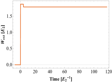
(a) External Work

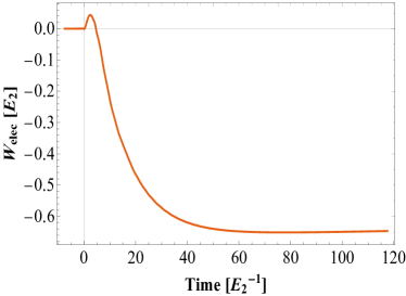
(b) Electrochemical Work

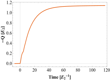
(c) Total Heat Dissipated

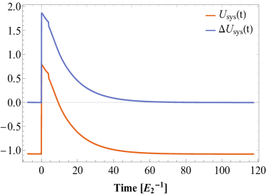
(d) Internal Energy (and consistency check)

Figure 3: The time-dependent energetics of the Electrochemical Pump depicted schematically in Fig. 2. (a) Total Work done by external drive versus time, (b) total Electrochemical Work done versus time, (c) total Heat dissipated into reservoirs versus time, and (d) Internal Energy $U_{sys}$ (in orange) and $\Delta U_{sys}$ from integration of the RHS of the First Law equation (IV) (in blue) versus time. For the results shown, we have used $\hbar=1$ and we set the on-site energy on the left and right dots $\{E_{1},E_{2}\}=\{-1,1\}$ so that the difference in the on-site energies of the two dots is $\Delta E=E_{2}-E_{1}=2$ in units of $E_{2}$. The dot hybridization is set to $w=\Delta E/5$ and the coupling to the reservoirs is taken as $\Gamma=w/5$. The chemical potential and temperatures of the reservoirs are set $-\mu_{1}=\mu_{2}=0.5$ in units of $E_{2}$ and $k_{B}T_{1}=k_{B}T_{2}=0.016$ in units of $E_{2}$, respectively. The pulse amplitude is set equal to the difference in the on-site energies $\delta=\Delta E$ and the pulse duration is set $\tau=\pi/2w$ ($\pi$-pulse).

For the setup described, if the electrochemical potentials of the reservoirs are biased such that $\mu_{1}>E_{1}$ and $\mu_{2}<E_{2}$, electrons can be pumped uphill from the left to the right reservoir. A schematic of the chemical pump configuration is shown in Fig. 2. In this configuration, the Temperatures $T_{1}\,,T_{2}$ of the reservoirs are set to very low values to suppress any thermal excitations from contributing to the operation. The thermodynamic cycle for the pump involves the electron tunneling from the left reservoir to dot 1 followed by the pulse raising its energy to bring it into resonance with dot 2. The $\pi$-pulse ensures a maximum probability of dot 2 capturing the electron at the end of the pulse, which is followed by the electron tunneling out into the right reservoir. The machine relaxes back to its initial state at late times, at which point we can calculate the efficiency of the electrochemical pump as

$$\eta_{EP}=\frac{|W_{elec}(t\rightarrow\infty)|}{|W_{ext}(t\rightarrow\infty)|}.$$ (91)

The full Hamiltonian for this configuration is given by Eq. (1), where the System Hamiltonian is

$$H_{S}(t)=E_{1}(t)d_{1}^{\dagger}d_{1}+E_{2}d_{2}^{\dagger}d_{2}+w(d_{1}^{\dagger}d_{2}+d_{2}^{\dagger}d_{1})\,,$$ (92)

with the Reservoir Hamiltonian given by

$$H_{R}=\sum_{i=1,2}\sum_{k\in i}\epsilon_{k}c_{k}^{\dagger}c_{k}\,,$$ (93)

and the coupling is such that the $i^{th}$ dot is only coupled to the $i^{th}$ reservoir

$$H_{SR}=\sum_{k\in 1}(V_{k1}c_{k}^{\dagger}d_{1}+h.c.)+\sum_{k\in 2}(V_{k2}c_{k}^{\dagger}d_{2}+h.c.)\,.$$ (94)

Finally, the time dependence of the system is encoded in the left dot as

$$E_{1}(t)=\begin{cases}E_{1}&t<0,\\ E_{1}+\delta&0\leq t<\tau,\\ E_{1}&t\geq\tau.\par\end{cases}$$ (95)

Fig. 3 shows plots of all the thermodynamic quantities entering the First Law as functions of time. We note that we have plotted the integrated thermodynamic quantities here instead of the time-derivatives that appear in the First Law [Eq. (IV)], so that we have the total external work done on the system $W_{ext}(t)=-i\int_{-\infty}^{t}\,dt\mathbb{Tr}\{\dot{H}^{(1)}_{S}(t)G^{<}(t,t)\}$, the total electrochemical work done on the system $W_{elec}(t)=\int_{-\infty}^{t}\,dt[\sum_{\alpha}-\mu_{\alpha}I_{\alpha}^{(0)}(t)]$, and the total heat dissipated into the reservoirs $-Q(t)=\int_{-\infty}^{t}\,dt(\sum_{\alpha}I_{\alpha}^{Q}(t))$. All the energies reported for this setup are in units of the on-site energy of the right dot $E_{2}$ and time is in units of $E_{2}^{-1}$.

The total external work done by the drive $W_{ext}(t)$, (Fig. 3a) follows the expected instantaneous rise of the pulse at $t=0$ to a value of $1.87$, indicating that work is done on the system by the drive. $W_{ext}(t)$ remains at this constant value for the duration of the pulse $\tau$, followed by a slight instantaneous decrease at $t=\tau$. This can be explained by noting that there is a small but finite probability for the electron being on dot 1 at the end of the $\pi$-pulse. This results in work being done by the system on the drive as the energy of the first dot is lowered back to its initial value, appearing as a negative contribution. The external work done remains constant at a value of $1.78$ thereafter since the drive is inactive for $t>\tau$.

As the pulse starts, the electrochemical work $W_{elec}(t)$, (Fig. 3b) is done on the system as the particle current flows mostly into the left reservoir initially. At a certain time $t>\tau$ the electrochemical work becomes negative indicating that electrochemical work is now done by the system as the particle current starts to flow mostly into the right reservoir. It increases in magnitude for some time and eventually attains a constant value of $-0.65$ at late times as the particle currents flowing into the reservoirs relax to $0$. For the complete cycle, electrochemical work is thus done by the system in transferring an electron from the reservoir with the lower chemical potential $\mu_{1}$ to the one with the higher chemical potential $\mu_{2}$. With the late time values of $W_{elec}(t)$ and $W_{ext}(t)$, we can see that the efficiency of the electrochemical pump $\eta_{EP}$ is about $36.5\%$.

The total heat dissipated into the reservoirs $-Q(t)$ (Fig. 3c) always remains positive implying that heat is only ever flowing into the reservoirs in the electrochemical pump configuration for the parameters chosen. This can be explained by noting that the (steady-state) heat flowing into the $i^{th}$ reservoir goes as $~{}(\omega_{i}-\mu_{i})v_{i}f_{i}(\omega)$, where $v_{i}$ is the velocity of the electron [79]. The levels in the numerics are biased such that $(\omega_{i}-\mu_{i})v_{i}$ always remains positive for both reservoirs, no matter which direction the electron is moving. The pronounced knee at $t=\tau$ is due to the opening up of another transport channel at the first dot in the form of a hole channel once the electron has been captured by the second dot at the end of the pulse and the left dot is in an empty state. The total heat dissipated asymptotes to a constant value of $1.17$ at late times.

We finally plot the internal energy $U_{sys}(t)$ (Fig. 3d) and note that it matches up well with the plot of the sum of all the terms appearing on the right hand side of the First Law i.e., $\Delta U_{sys}(t)=W_{ext}(t)+W_{elec}(t)+Q(t)$. The offset is expected since we have plotted $U_{sys}(t)$ directly from the Eqs. (63) and (71), which are expressions for energy, whereas the plot of $\Delta U_{sys}(t)$ was generated by integration of the current formulas where the constant of integration was set to $0$.

VI.2.1 Spatio-Temporal Distribution of Energy—Electrochemical Pump

Figure 4: Schematic representation of the driven double quantum dot system (red box) discussed in Secs. VI.2.1 and VI.3.1, now coupled specifically to semi-infinite tight-binding chains. The left and right dots are labeled as D1 and D2, respectively, and the chain sites on the left and right reservoirs are labelled 1L, 2L,… and 1R, 2R,…, respectively. Only the site $1L$ is directly coupled to $D1$ and only the site $1R$ is directly coupled to $D2$.

To develop a finer-grained understanding of the operation of this strongly-driven quantum machine, we investigate the spatio-temporal distribution of energy using the theory of energy density developed in Sec. IV.1. We work with essentially the same setup that was used in the preceding paragraphs for the integrated thermodynamic quantities, but now with a specific model for the reservoirs: 1D tight-binding chains. The System Hamiltonian $H_{S}(t)$ is chosen the same as before [Eq. (92)]. The Reservoir Hamiltonian is

$$H_{R}=\sum_{\alpha=L,R}\Bigg{[}\sum_{j=1}^{\infty}\epsilon_{0}c_{j\alpha}^{\dagger}c_{j\alpha}+\sum_{j=1}^{\infty}t_{0}(c_{j\alpha}^{\dagger}c_{j+1\alpha}+h.c.)\Bigg{]}\,,$$ (96)

where $\epsilon_{0}$ is the on-site energy at any given site and $t_{0}$ is the hopping integral between nearest-neighbor sites on a given chain. The coupling Hamiltonian modelling the Interface is

$$H_{SR}=t\Bigg{[}(d_{1}^{\dagger}c_{1L}+h.c.)+(d_{2}^{\dagger}c_{1R}+h.c.)\Bigg{]}\,,$$ (97)

where $t$ is the coupling between the first site in the left reservoir $1L$ and the left dot, and that between the first site in the right reservoir $1R$ and the right dot. A schematic of this setup is given in Fig. 4.

We study the energy density of the system, defined in Eq. (61), as a function of time. The contributions of $H_{S}(t)$ and $H_{SR}$ to the energy density are evaluated using Eqs. (87) and (89), respectively. The tunneling-width matrices for the 1D tight-binding chains coupled to the double quantum dot system are [80, 81]

$$[\Gamma_{\alpha}(\omega)]_{ij}=\begin{cases}\frac{2t^{2}}{t_{0}}\Big{(}1-\Big{(}\frac{\epsilon_{0}-\hbar\omega}{2t_{0}}\Big{)}^{2}\Big{)}^{\frac{1}{2}}\delta_{i\alpha}\delta_{j\alpha},&|\hbar\omega-\epsilon_{0}|<2t_{0},\\ 0,&\text{otherwise}.\end{cases}$$ (98)

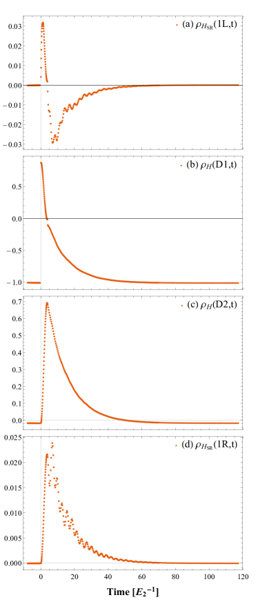
Figure 5: Plots of spatially resolved energy as a function of time for the Electrochemical Pump configuration for the same Hamiltonian parameters as those for Fig. 3. For the interfacial sites of both the reservoirs, we plot the contribution of the interface energy [Eq. (97)] denoted by $\rho_{H_{SR}}(1L,t)$ and $\rho_{H_{SR}}(1R,t)$ for the left and right reservoirs, respectively. For the two dots, we plot the total energy density as a function of time denoted by $\rho_{H}(D1,t)$ and $\rho_{H}(D2,t)$. The energies are in units of the on-site energy of the right dot $E_{2}$ and time is in units of $E_{2}^{-1}$in this configuration. Note that the energy scale for $\rho_{H_{SR}}(1L,t)$ and $\rho_{H_{SR}}(1R,t)$ (panels (a) and (d)) is different from that for $\rho_{H}(D1,t)$ and $\rho_{H}(D2,t)$ (panels (b) and (c)) in the figure.

The numerical results for the energy density for the electrochemical pump are shown in Fig. 5 for the system in the electrochemical pump configuration . We plot the total energy density for the two dots $D1$ and $D2$, and just the contribution of the coupling Hamiltonian $H_{SR}$ [Eq. (97)] to the energy density for the first sites $1L$ and $1R$ on the left and right reservoirs, respectively, which give half the energies of the left and right interfaces. Note that, by design, for the two dots we have $\rho_{H_{R}}(D1,t)=\rho_{H_{R}}(D2,t)=0$ and similarly for the sites on the reservoirs we have $\rho_{H_{S}}(1L,t)=\rho_{H_{S}}(1R,t)=0$.

The total energy on the left dot $\rho_{H}(D1,t)$ (Fig. 5b) rises instantaneously to its maximum positive value at the start of the pulse as the external drive does work on the dot. As the electron Rabi oscillates onto the right dot, the energy on the left dot begins to decrease and at the end of the pulse becomes zero and then asymptotes to its intial value as the initial conditions of the system are established again at late times. The Rabi oscillations of the system become more evident for the case of a $3\pi$-pulse, as seen in Fig. LABEL:fig:Usys_den_3tau, where we have again plotted the energy density [Eq. (61)] for both the dots and first sites of both reservoirs.

The interfacial energy at the first site in the left reservoir $\rho_{H_{SR}}(1L,t)$ (Fig. 5a) rises and falls in response to changes in the energy on Dot 1. This “in-phase with $D1$” behavior can be understood by noting that $H_{SR}$ models the covalent bond between the dot and the first site on the chain which is equally shared between the two. Negative (positive) bond energies correspond to bonding (anti-bonding) character of the Dot-Reservoir interface. The bond energy tends to zero at long times as the system relaxes to its initial state wherein the occupancy of Dot 1 is nearly unity so that the hybridization with the left Reservoir tends to zero. The oscillatory behavior during the relaxation is a signature of the Rabi oscillations between the two dots $D1$ and $D2$, which are enhanced in frequency (but suppressed in amplitude) when the pulse is inactivated.

The energy on the right dot $\rho_{H}(D2,t)$ (Fig. 5c) rises as the electron Rabi oscillates onto it from the left dot and begins to decrease as the electron tunnels out onto the first site in the right reservoir, eventually relaxing back to its zero initial value. The interfacial coupling energy on the first site in the right reservoir $\rho_{H_{SR}}(1R,t)$ (Fig. 5d) can be understood similarly to that on site $1L$ within the bonding picture discussed in the previous paragraph. As the electron tunnels onto $1R$ from the right dot the energy there increases followed by an asymptotic decrease to its initial value again almost mimicking the temporal behavior at $D2$.

VI.3 Heat Engine

Figure 6: Schematic representation of a Heat Engine based on Rabi Oscillations between states of a double quantum dot. The left and right dots in the system have on-site energies $E_{1}$ and $E_{2}$, respectively, and are dynamically coupled by a time-dependent hopping term $w(t)$. The left dot is driven by a rectangular pulse of width $\tau$ and strength $\delta$. Each dot is coupled with the same Tunneling width matrix element $\Gamma$ to a Reservoir. The Reservoirs are modeled as non-interacting, Fermionic, semi-infinite systems at Temperatures $T_{1}$ and $T_{2}$ for the left and right reservoirs, respectively, with $T_{2}>T_{1}$. The cycle of operation of the heat engine is denoted by the dashed purple arrows.

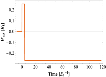
(a) External Work

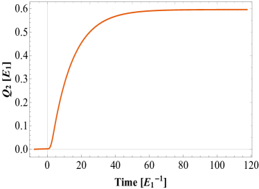
(b) Heat extracted from Right Reservoir

(c) Electrochemical Work

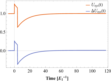
(d) Internal Energy (and consistency check)

Figure 7: The Time-dependent energetics of the Heat Engine depicted schematically in Fig. 6. (a) Total Work done by external drive versus time, (b) Heat extracted from the right (hot) Reservoir, (c) total Electrochemical Work done versus time, and (d) Internal Energy (in orange) and RHS of the First Law equation (IV) (in blue) versus time. For the results shown, we have used $\hbar=1$ and we set the on-site energy on the left and right dots to $\{E_{1},E_{2}\}=\{1,3\}$ so that the difference in the on-site energies of the two dots is $\Delta E=E_{2}-E_{1}=2$ in units of $E_{1}$. The dot hybridization (when non-zero during the pulse) is set $w=\Delta E/5$ and the coupling to the reservoirs is taken as $\Gamma=w/5$. The chemical potentials and temperatures of the reservoirs are set to $\mu_{1}=\mu_{2}=0$ and $\{k_{B}T_{1},k_{B}T_{2}\}=\{0.5,3.6\}$ in units of $E_{1}$, respectively. The pulse amplitude is set equal to the difference in the on-site energies $\delta=\Delta E$ and the pulse duration is set $\tau=\pi/2w$ ($\pi$-pulse).

For the heat engine configuration, the temperatures are raised to significant unequal values $(T_{2}>T_{1})$ comparable in magnitude to the system energy levels, and the chemical potentials of both the reservoirs are set to zero, $\mu_{1}=\mu_{2}=0$. Furthermore, in addition to the left dot energy, the inter-dot coupling is now a function of time $w\rightarrow w(t)$. Specifically, it is activated to a constant value $w$ only during the pulse and is zero before and after it. This is done to suppress heat flow into the reservoirs in the quiescent state of the machine. The efficiency of the cycle is

$$\eta_{HE}=\frac{|W_{ext}(t\rightarrow\infty)|}{|Q_{2}(t\rightarrow\infty)|},$$ (99)

where $Q_{2}(t\rightarrow\infty)$ is the heat extracted from the right reservoir at late times.

Again, the full Hamiltonian for this configuration is given by Eq. (1) and the System Hamiltonian is

$$H_{S}(t)=E_{1}(t)d_{1}^{\dagger}d_{1}+E_{2}d_{2}^{\dagger}d_{2}+w(t)(d_{1}^{\dagger}d_{2}+d_{2}^{\dagger}d_{1}),$$ (100)

with the Reservoir and Coupling Hamiltonians exactly the same as in the electrochemical pump case given by Eqs. (93) and (94), respectively. As before, the rectangular pulse acts only on the left dot with $E_{1}(t)$ given by Eq. (95), and the time-dependent inter-dot coupling is

$$w(t)=\begin{cases}0&t<0,\\ w&0\leq t<\tau,\\ 0&t\geq\tau.\par\end{cases}$$ (101)

In the heat engine configuration, the electron transport path is essentially reversed from the pump configuration. The electron tunnels in from the right reservoir onto the right dot, Rabi Oscillates onto the left dot, is lowered to energy $E_{1}$ at the end of the pulse, and tunnels out into the left reservoir, accomplishing engine operation. A schematic for the engine is given in Fig. 6.

The time-dependent energetics shown in Fig. 7, where all the energies are reported in units of the on-site energy of the left dot $E_{1}$ and time is in units of $E_{1}^{-1}$, demonstrate that external work $W_{ext}(t)$ (Fig. 7a) is now done by the engine on the drive as the left dot is lowered at the end of the pulse. For the parameters chosen $W_{ext}(t)$ at late times attains a constant value of $-0.18$. This work is done by extracting heat $Q_{2}(t)$ (Fig. 7b) from the hot reservoir at $T_{2}$, and eventually attains a constant value of $-0.60$ at late times after the pulse and inter-dot coupling are inactivated.

By design, no net electrochemical work is done (Fig. 7c) since we had set the chemical potentials of both the reservoirs to $0$ in this configuration. Finally, the left and right hand sides of the First Law are again in good agreement (Fig. 7d), up to a constant of integration offset. For the parameters chosen, the heat engine operates at an efficiency $\eta_{HE}$ of about $46.5\%$ which is close to $53\%$ of Carnot efficiency.

VI.3.1 Spatio-Temporal Distribution of Energy—Heat Engine

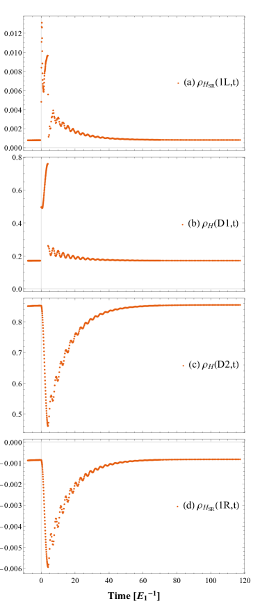
Figure 8: Plots of spatially resolved energy as a function of time for the Heat Engine configuration for the same Hamiltonian parameters as those for Fig. 7. For the interfacial sites on both the reservoirs, we plot the contribution of the interface energy [Eq. (97)] denoted by $\rho_{H_{SR}}(1L,t)$ and $\rho_{H_{SR}}(1R,t)$ for the left and right reservoirs, respectively. For the two dots, we plot the total energy density as a function of time denoted by $\rho_{H}(D1,t)$ and $\rho_{H}(D2,t)$. The energies are in units of the on-site energy of the right dot $E_{1}$ and time is in units of $E_{1}^{-1}$in this configuration. Note that the energy scale for $\rho_{H_{SR}}(1L,t)$ and $\rho_{H_{SR}}(1R,t)$ (panels (a) and (d)) is different from that for $\rho_{H}(D1,t)$ and $\rho_{H}(D2,t)$ (panels (b) and (c)) in the figure.

Fig. 8 gives the results for the spatiotemporal distribution of the energy of the machine in the Heat Engine configuration. For these results, the system Hamiltonian is the same as Eq. (100) used for the integrated thermodynamic quantities in the preceding paragraphs, and the functional form of the reservoir and coupling Hamiltonians is kept the same as that in the electrochemical pump case, Eqs. (96) and (97).

We again see the total energy for the left dot $\rho_{H}(D1,t)$ (Fig. 8b) rise instantaneously as the pulse is activated at $t=0$. It increases further to its maximum value as the electron Rabi oscillates from the right dot to the left dot. The energy on the left dot decreases as the electron tunnels out into the left reservoir, eventually asymptoting to its initial value at late times.

On the first site on the left reservoir, the interfacial energy $\rho_{H_{SR}}(1L,t)$ (Fig. 8a) rises first at $t=0$ in response to the activation of the pulse at the left dot, reflecting again the fact that $H_{SR}$ models the bond between the system and reservoir. The energy rises for a second time in response to the Rabi oscillation of the electron onto the left dot from the right dot, and yet again for a third and final time as the electron tunnels onto the first site on the left reservoir itself. As initial conditions are re-established, the coupling energy again assumes its initial value.

On the right dot, the energy $\rho_{H}(D2,t)$ (Fig. 8c) begins to decrease upon the activation of the pulse as the electron tunnels onto the left dot. It asymptotes back to its initial value as another electron tunnels in from the right reservoir and initial conditions are re-established. Again, the interfacial contribution to the energy $\rho_{H_{SR}}(1R,t)$ (Fig. 8d) on the first site on right reservoir almost mimics the behaviour at the right dot.

VII Conclusions

Formulation of the First Law of Thermodynamics requires proper definitions of Work, Heat, and Internal Energy. While the definition of External Work was established early on in Quantum Thermodynamics [49, 22], the latter two concepts have proven problematic for open quantum systems driven out of equilibrium [22, 23, 24, 25, 26, 27, 28]. In this article, we have shown that the proper definition of the Internal Energy operator $U_{sys}(t)$ for an open quantum system is the partition of the Hamiltonian operator onto the system Hilbert space, confirming the validity of the so-called half-and-half partition [23, 24], $U_{sys}(t)=H_{S}(t)+\frac{1}{2}H_{SR}$, wherein the internal energy of the system is the sum of the system Hamiltonian and half of the coupling Hamiltonian describing the System-Reservoir interface. Furthermore, we have been able to identify the Electrochemical Work done on the system and the Heat flowing out of the system into the environment by employing a key insight from Mesoscopics—that far away from the local driving and coupling of the system, the reservoirs remain arbitrarily close to equilibrium. This allows the Electrochemical Work and Heat to be properly defined for open quantum systems driven far from equilibrium, although there is a transient component of the energy flux, carried in particular by phonons, that is not identifiable as heat per se except for steady-state or slowly-varying driving conditions.

Our definition (60) of Internal Energy agrees with that proposed by Ludovico et al. [23] for the specific model of a single sinusoidally driven Fermionic resonant level coupled to a single reservoir (supported in the subsequent work of Bruch et al. [24]), as well as with that put forward by Stafford and Shastry [64, 34, 35] for an independent Fermion system in steady state, but disagrees with those put forward by Esposito et al. [25], Strasberg and Winter [26], and Lacerda et al. [27]. We remark that our definition of $U_{sys}(t)$ based on Hilbert-space partition appears to coincide with the definition of Internal Energy advocated in Ref. [24]—based on the $H_{S}$-dependent part of the total energy—in the broad-band limit only, but our definition remains valid outside the broad-band limit.

We have derived fully general expressions for all the terms appearing in the First Law using the formalism of non-equilibrium Green’s functions (NEGF). In our analysis, the system-reservoir coupling can be arbitrarily strong, and our analysis can be readily extended to the general case where the system, coupling, and reservoir are all explicitly time-dependent (see Appendix LABEL:full_tdpt_generalize_app). Furthermore, our formal results incorporate electronic and phononic degrees of freedom in both the system and the reservoir as well as electron-electron, electron-phonon, and phonon-phonon interactions in the system. In our analysis, the external electromagnetic field used to drive the electron-phonon system is treated classically, which allows for absorption and stimulated emission of energy quanta, but does not allow spontaneous emission or radiative heat transfer [83].

We also studied the spatio-temporal distribution of the energy in a strongly-driven time-dependent open quantum system, shedding light on the internal dynamics of the system as well as on the evolution of the system-reservoir interface. The interface contribution to the internal energy of the system was shown to be localized at the junctions between the system and the reservoirs. For the case of a metallic reservoir in the nearest-neighbor tight-binding model, with only nearest-neighbor bonds to the system, the interface energy was found to be entirely localized on the system-reservoir bonds. The sign of the interface energy can vary from negative to positive, corresponding to bonding or antibonding character of the interface, respectively.

We applied our formal results to a strongly driven quantum machine utilizing Rabi Oscillations between states of a double quantum dot coupled to metallic reservoirs. We presented a full thermodynamic analysis of the machine’s operation as both an electrochemical pump and a heat engine, illustrating the utility of our theoretical framework and the power of our computational approach based on NEGF.

It should be remarked that although the First Law clearly holds at the level of quantum statistical averages, provided the energetics are partitioned properly, one cannot expect it to hold at the level of individual quantum trajectories, since the operators for internal energy, heat current, and chemical power (among others) do not commute, and hence these are incompatible observables [22, 84]. In particular, in addition to thermal fluctuations, there exist also quantum fluctuations of the various energetic factors appearing in the First Law due to the generalized uncertainty principle for non-commuting observables.

It is hoped that our very general derivation of the First Law of Thermodynamics in time-dependent open quantum systems, illustrated with applications of our theory to specific examples of model quantum thermal machines, will help to resolve once and for all the controversy over the validity of First Law of Thermodynamics in open quantum systems.

VIII Acknowledgments

It is a pleasure to acknowledge several helpful discussions with Caleb M. Webb, Marco A. Jimenez-Valencia, and Carter S. Eckel during various stages of this work. We also thank J. M. van Ruitenbeek for suggesting the valuable generalization of incorporating phonons in our model. This work was partially supported by the U.S. Department of Energy (DOE), Office of Science under Award No. DE-SC0006699. After submission of the first version of this manuscript, we became aware of Ref. [85], which addresses some issues similar to those considered in this article.

Appendix A Some details about Entropy and the Hilbert Space partition

This appendix provides some additional details of the analysis of entropy and Hilbert space partition given in Sec. III.3.

A.1 Derivation of Eq. (32)

Eq. (32) follows straightforwardly from Eq. (31) using the properties of the density matrix and perturbation theory. In its eigenbasis, the density matrix may be written

$$\rho=\sum_{\nu}\lambda_{\nu}|\lambda_{\nu}\rangle\langle\lambda_{\nu}|,$$ (106)

with $\sum_{\nu}\lambda_{\nu}=1$. A small deviation of $\rho$ from an initial density matrix $\rho_{0}$ is given to linear order by

$$d\rho=\sum_{\nu}\left[d\lambda_{\nu}|\lambda_{\nu}^{0}\rangle\langle\lambda_{\nu}^{0}|+\lambda_{\nu}^{0}|d\lambda_{\nu}\rangle\langle\lambda_{\nu}^{0}|+\lambda_{\nu}^{0}|\lambda_{\nu}^{0}\rangle\langle d\lambda_{\nu}|\right],$$ (107)

where $\langle d\lambda_{\nu}|\lambda_{\nu}^{0}\rangle=0$ without loss of generality. The linear deviation of the entropy is

$$dS=-\sum_{\nu}d\lambda_{\nu}\ln\lambda_{\nu}^{0}-\sum_{\nu}d\lambda_{\nu},$$ (108)

where the second term on the rhs vanishes due to the invariance of the trace of $\rho$. Finally,

$${\rm Tr}\{d\rho\ln\rho_{0}\} = \sum_{\nu}\langle\lambda_{\nu}^{0}|d\rho|\lambda_{\nu}^{0}\rangle\ln\lambda_{\nu}^{0}$$ (109)

$$= \sum_{\nu}d\lambda_{\nu}\ln\lambda_{\nu}^{0},$$

where the second line follows from Eq. (107) because $\langle d\lambda_{\nu}|\lambda_{\nu}^{0}\rangle=0$. This completes the proof of Eq. (32)

A.2 Derivation of Eq. (40)

Using Eq. (36) and $\omega A(\omega)=h^{(1)}A(\omega)$, Eq. (40) may be written

$$TdS_{\gamma}=\int d\omega\mathbb{Tr}^{(1)}\{\Pi_{\gamma}(h^{(1)}-\mu)A(\omega)\}df(\omega).$$ (110)

Because $[h^{(1)},A]=0$, we can rewrite the trace

$$\mathbb{Tr}^{(1)}\{\Pi_{\gamma}h^{(1)}A(\omega)\} = \frac{1}{2}\mathbb{Tr}^{(1)}\{\Pi_{\gamma}\{h^{(1)},A(\omega)\}\}$$ (111)

$$= \mathbb{Tr}^{(1)}\{\left.h^{(1)}\right|_{\gamma}A(\omega)\},$$

where the second line used Eq. (41) and the cyclic property of the trace. The expectation value of the Hamiltonian partitioned on subsystem $\gamma$ in thermal equilibrium is

$$\langle\left.H^{(1)}\right|_{\gamma}\rangle = \int d\omega\mathbb{Tr}^{(1)}\{\left.h^{(1)}\right|_{\gamma}A(\omega)\}f(\omega)$$ (112)

$$= -i\mathbb{Tr}^{(1)}_{\gamma}\left\{h^{(1)}(t)G^{<}(t,t)\right\},$$

where the second line holds also out of equilibrium. Finally, including only the change in the statistical factors but not the change in the Hamiltonian itself,

$$\int d\omega\mathbb{Tr}^{(1)}\{\left.h^{(1)}\right|_{\gamma}A(\omega)\}df(\omega)=d\langle\left.H^{(1)}\right|_{\gamma}\rangle-\langle\left.dH^{(1)}\right|_{\gamma}\rangle.$$ (113)

This completes the derivation of Eq. (40).

A.2.1 Phonon analysis

For the case of a harmonic phonon system, Eq. (35) takes the form

$$TdS_{\gamma}^{ph}=\int d\omega\mathbb{Tr}^{(1)}_{\gamma}\{A^{ph}(\omega)\}\hbar\omega\,df^{Planck}(\omega),$$ (114)

where $A^{ph}(\omega)=\delta(\omega-\sqrt{K})$ and the harmonic interaction matrix $K$ was defined in Eq. (6). Eq. (114) may be integrated to obtain the phonon subsystem entropy in equilibrium

$$S^{ph}_{\gamma}=\int d\omega\mathbb{Tr}^{(1)}_{\gamma}\{A^{ph}(\omega)\}s_{-}(\omega),$$ (115)

which is non-singular and respects the 3rd Law of Thermodynamics as $T\rightarrow 0$, where

$$s_{-}(\omega)=\beta\hbar\omega f^{Planck}(\omega)-\ln(1-e^{-\beta\hbar\omega}).$$ (116)

By arguments similar to those given above, one can readily show that the phonon contributions to the entropy, work, and internal energy changes also satisfy Eq. (40) in the harmonic approximation (with $\mu=0$ for phonons).

A.3 Partition of the two-body interactions

The electron-electron interaction term may be treated along the lines of Eq. (112) with the help of the Coulomb self-energy $\Sigma_{C}$. The expectation value of the electronic Hamiltonian, including electron-electron interactions is [87]

$$\langle H(t)\rangle=-i\mathbb{Tr}^{(1)}\left\{h^{(1)}(t)G^{<}(t,t)+\frac{1}{2}\int dt^{\prime}\left[\Sigma_{C}(t,t^{\prime})G(t^{\prime},t)\right]^{<}\right\}.$$ (117)

Using the Langreth rules [31], this may be expressed as

$$\langle H(t)\rangle=-i\mathbb{Tr}^{(1)}\left\{h^{(1)}(t)G^{<}(t,t)+\frac{1}{2}\int dt^{\prime}\left[\Sigma_{C}^{R}(t,t^{\prime})G^{<}(t^{\prime},t)+\Sigma_{C}^{<}(t,t^{\prime})G^{A}(t^{\prime},t)\right]\right\}.$$ (118)

The mean energy of subsystem $\gamma$ is then

$$\langle\left.H\right|_{\gamma}(t)\rangle=-\frac{i}{2}\mathbb{Tr}^{(1)}_{\gamma}\left\{\{h^{(1)},(t)G^{<}(t,t)\}+\frac{1}{2}\int dt^{\prime}\left[\{\Sigma_{C}^{R}(t,t^{\prime}),G^{<}(t^{\prime},t)\}+\{\Sigma_{C}^{<}(t,t^{\prime}),G^{A}(t^{\prime},t)\}\right]\right\}.$$ (119)

Because two-body interactions occur only within the system (by construction), the Coulomb self-energy is a system-diagonal matrix in the one-particle Hilbert space. The two-body interactions therefore do not contribute to the partition of the Hamiltonian onto the reservoirs, confirming Eq. (43). This result may also be obtained directly by partitioning $H^{(2)}$, as discussed in Ref. [36].

In a similar way, it can be shown that phonon anharmonic terms and electron-phonon interactions, occuring only within the system, do not contribute to the partition of the Hamiltonian onto the reservoirs.

Appendix B Derivation of the NEGF formulas for all First Law quantities

This appendix gives details of the derivations of the key NEGF results presented in Sec. V.

B.1 Computations in the NEGF formalism

Before giving the details of specific results we briefly review here the general procedure employed in computing the Non-Equilibrium Green’s functions. Within the framework of NEGF, the Retarded Green’s function $G^{R}(t,t^{\prime})$, which describes the dynamics of the system, can be computed using the Dyson Equation lcr G^R(t,t’)= G^R_0(t,t’)+∫_-∞^∞  dt_1∫_-∞^∞  dt_2 G^R_0(t,t_1)Σ^R(t_1,t_2)G^R(t_2,t’)  , where $G^{R}_{0}(t,t^{\prime})$ is the Green’s function for the non-interacting and uncoupled system and the Self-Energy function which encodes the interactions and tunneling is given by

$$\Sigma^{R}(t,t^{\prime})=\Sigma^{R}_{int}+\Sigma^{R}_{tun}(t,t^{\prime})\,,$$ (120)

where $\Sigma^{R}_{int}$ is the retarded interaction self-energy of the system (for example, the Coulomb self-energy) and the retarded tunneling self-energy is given by

$$\Sigma^{R}_{tun}(t,t^{\prime})=\sum_{\alpha}\int_{-\infty}^{\infty}\,\frac{d\omega}{2\pi}e^{-i\omega(t-t^{\prime})}[\Lambda_{\alpha}(\omega)-\frac{i}{2}\Gamma_{\alpha}(\omega)]\,,$$ (121)

with $\Lambda_{\alpha}(\omega)=\mathcal{P}\int_{-\infty}^{\infty}\,\frac{d\omega^{\prime}}{2\pi}\frac{\Gamma_{\alpha}(\omega^{\prime})}{\omega-\omega^{\prime}}$, where $\mathcal{P}$ denotes the Principal Value [see, for instance, Eq. ($2.26$) in [31]]. The Lesser Green’s function $G^{<}(t,t^{\prime})$, which describes the occupation of the system, can be computed using the Keldysh Equation

$$G^{<}(t,t^{\prime})=\int_{-\infty}^{\infty}\,dt_{1}\int_{-\infty}^{\infty}\,dt_{2}G^{R}(t,t_{1})\Sigma^{<}(t_{1},t_{2})G^{A}(t_{2},t^{\prime})\,,$$ (122)

where we have omitted the so-called memory term [see, for instance, Eq. (5.11) in [30]] since it is not relevant for the protocols we consider in this article, and the lesser Self-Energy function is

$$\Sigma^{<}(t,t^{\prime})=\Sigma^{<}_{int}(t,t^{\prime})+i\sum_{\alpha}\int_{-\infty}^{\infty}\,\frac{d\omega}{2\pi}e^{-i\omega(t-t^{\prime})}f_{\alpha}(\omega)\Gamma_{\alpha}(\omega)\,.$$ (123)

The two-body Green’s function $G^{(2)}(t,t)$ appearing in Eq. (64) can be evaluated directly using the Bethe-Salpeter equation [31], or the contribution from electron-electron interactions to Eq. (63) can be evaluated using the Coulomb self-energy and the one-body Green’s function, as in Eqs. (118)–(119). The electron-phonon Green’s function $G^{(2),el-ph}(t,t)$ and the higher-order phonon Green’s functions such as $D^{ahm}(t,t,t)$, appearing in Eqs. (67) and (70), can be evaluated using the well-developed theory of electron-phonon and phonon-phonon interactions [88, 89].

B.2 Electronic Heat current

Here we give the details of the derivation of the electronic heat current formula in terms of the System Green’s functions using the Nonequilibrum Green’s function (NEGF) formalism [69, 70, 71, 30, 31]. (The calculation of the interface internal energy [Eq. (71)] proceeds in a nearly parallel fashion.)

To derive the conventional component of heat current formula [Eq. (V.4)], we begin with the electronic heat current given in terms of expectation values in Eq. (51). We then use the the lesser Tunneling Green’s functions (defined in V.5) $G^{<}_{nk}(t,t^{\prime})=i\langle c_{k}^{\dagger}(t^{\prime})d_{n}(t)\rangle$ and $G^{<}_{kn}(t,t^{\prime})=i\langle d_{n}^{\dagger}(t^{\prime})c_{k}(t)\rangle$, where, to lighten notation we write $G^{<}_{tun,nk}(t,t^{\prime})$ simply as $G^{<}_{nk}(t,t^{\prime})$, and noting that at equal times $G^{<}_{nk}(t,t)=-[G^{<}_{kn}(t,t)]^{*}$, to write the heat current as

$$I_{\alpha,el}^{Q,conv}(t)=\frac{-2}{\hbar}\mathbb{Re}\Bigg{[}\sum_{k\in\alpha,n}(\epsilon_{k}-\mu_{\alpha})V_{kn}^{el}G^{<}_{nk}(t,t)\Bigg{]}\,.$$ (124)

The NEGF prescription tells us that $G^{<}_{nk}(t,t^{\prime})$ will be a component of the Contour-Ordered Tunneling Green’s function

$$G^{\mathcal{T}}_{nk}(\tau,\tau^{\prime})=-i\langle\mathcal{T}(d_{n}(\tau)c_{k}^{\dagger}(\tau^{\prime}))\rangle\,,$$ (125)

where $\tau$ is the contour time. The equation of motion of the Contour-Ordered Tunneling Green’s function is

$$-i\hbar\frac{\partial}{\partial\tau^{\prime}}G^{\mathcal{T}}_{nk}(\tau,\tau^{\prime})=\epsilon_{k}G^{\mathcal{T}}_{nk}(\tau,\tau^{\prime})+\sum_{m}G^{\mathcal{T}}_{nm}(\tau,\tau^{\prime})(V^{el}_{km})^{*}\,,$$ (126)

where $G^{\mathcal{T}}_{nm}(\tau,\tau^{\prime})=-i\langle\mathcal{T}(d_{n}(\tau)d_{m}^{\dagger}(\tau^{\prime}))\rangle$ is the Contour-Ordered System Green’s function and we get

$$G^{\mathcal{T}}_{nk}(\tau,\tau^{\prime})=\frac{1}{\hbar}\sum_{m}\int\,d\tau_{1}G^{\mathcal{T}}_{nm}(\tau,\tau_{1})(V^{el}_{km})^{*}g^{\mathcal{T}}_{kk}(\tau_{1},\tau^{\prime})\,,$$ (127)

using the equation of motion of the uncoupled Contour-Ordered reservoir Green’s function $g_{kk}^{\mathcal{T}}(\tau,\tau^{\prime})=-i\langle c_{k}(\tau)c^{\dagger}_{k}(\tau^{\prime})\rangle$. The physical lesser component of the Contour-Ordered Tunneling Green’s function [Eq. (127)] can be found using the so-called Langreth rules [30, 31], giving lcr G^¡_nk(t,t’)=1ℏ∑_m ∫ dt_1 (V^el_km)^*[G^R_nm(t,t_1)g^¡_kk(t_1,t’) +G^¡_nm(t,t_1)g^A_kk(t_1,t’)]  .
& The lesser and advanced uncoupled Reservoir Green’s functions are given by

$$g^{<}_{kk}(t,t^{\prime})=i\langle c^{\dagger}_{k}(t^{\prime})c_{k}(t)\rangle=if(\epsilon_{k}^{0})\exp(\frac{-i}{\hbar}\epsilon_{k}(t-t^{\prime}))$$ (128)

and lcr g^A_kk(t,t’)=iθ(t’-t)⟨{c_k(t),c^†_k(t’)}⟩=iθ(t’-t)exp(-iℏϵ_k(t-t’))  , respectively, where

$$f(\epsilon_{k}^{0})=\frac{1}{e^{\beta_{\alpha}(\epsilon_{k}^{0}-\mu)}+1}$$ (129)

is the Fermi-Dirac distribution function. Putting this all together, we can write lcr I_α,el^Q,conv(t)= 2ℏ𝕀𝕞[∑_k∈α,n,m(ϵ_k-μ_α)∫_-∞^t  dt_1{e^-iℏϵ_k(t_1-t)V^el_kn(V

References

- Binder et al. [2018] F. Binder, L. A. Correa, C. Gogolin, J. Anders, and G. Adesso, eds., Thermodynamics in the Quantum Regime: Fundamental Aspects and New Directions, Fundamental Theories of Physics, Vol. 195 (Springer International Publishing, Cham, 2018).
- Shastry et al. [2020] A. Shastry, S. Inui, and C. A. Stafford, Scanning tunneling thermometry, Physical Review Applied 13, 024065 (2020).
- Mecklenburg et al. [2015] M. Mecklenburg, W. A. Hubbard, E. R. White, R. Dhall, S. B. Cronin, S. Aloni, and B. C. Regan, Nanoscale temperature mapping in operating microelectronic devices, Science (New York, N.Y.) 347, 629 (2015).
- Neumann et al. [2013] P. Neumann, I. Jakobi, F. Dolde, C. Burk, R. Reuter, G. Waldherr, J. Honert, T. Wolf, A. Brunner, J. H. Shim, D. Suter, H. Sumiya, J. Isoya, and J. Wrachtrup, High-precision nanoscale temperature sensing using single defects in diamond, Nano Letters 13, 2738 (2013), pMID: 23721106.
- Jeong et al. [2015] W. Jeong, S. Hur, E. Meyhofer, and P. Reddy, Scanning probe microscopy for thermal transport measurements, Nanoscale and Microscale Thermophysical Engineering 19, 279 (2015).
- Menges et al. [2016] F. Menges, P. Mensch, H. Schmid, H. Riel, A. Stemmer, and B. Gotsmann, Temperature mapping of operating nanoscale devices by scanning probe thermometry, Nature Communications 7, 10874 EP (2016), article.
- Shi et al. [2009] L. Shi, J. Zhou, P. Kim, A. Bachtold, A. Majumdar, and P. L. McEuen, Thermal probing of energy dissipation in current-carrying carbon nanotubes, Journal of Applied Physics 105, 104306 (2009).
- Kim et al. [2012] K. Kim, W. Jeong, W. Lee, and P. Reddy, Ultra-high vacuum scanning thermal microscopy for nanometer resolution quantitative thermometry, ACS Nano 6, 4248 (2012), pMID: 22530657.
- Lee et al. [2013] W. Lee, K. Kim, W. Jeong, L. A. Zotti, F. Pauly, J. C. Cuevas, and P. Reddy, Heat dissipation in atomic-scale junctions, Nature 498, 209 (2013).
- Gomès et al. [2015] S. Gomès, A. Assy, and P.-O. Chapuis, Scanning thermal microscopy: A review, physica status solidi (a) 212, 477 (2015).
- Cui et al. [2017] L. Cui, W. Jeong, S. Hur, M. Matt, J. C. Klöckner, F. Pauly, P. Nielaba, J. C. Cuevas, E. Meyhofer, and P. Reddy, Quantized thermal transport in single-atom junctions, Science (New York, N.Y.) 355, 1192 (2017).
- Mosso et al. [2017] N. Mosso, U. Drechsler, F. Menges, P. Nirmalraj, S. Karg, H. Riel, and B. Gotsmann, Heat transport through atomic contacts, Nat Nano 12, 430 (2017), letter.
- Toyabe et al. [2010] S. Toyabe, T. Sagawa, M. Ueda, E. Muneyuki, and M. Sano, Experimental demonstration of information-to-energy conversion and validation of the generalized Jarzynski equality, Nature Physics 6, 988 (2010), arxiv:1009.5287 [cond-mat.stat-mech] .
- Bérut et al. [2012] A. Bérut, A. Arakelyan, A. Petrosyan, S. Ciliberto, R. Dillenschneider, and E. Lutz, Experimental verification of Landauer’s principle linking information and thermodynamics, Nature 483, 187 (2012).
- Koski et al. [2014] J. V. Koski, V. F. Maisi, J. P. Pekola, and Dmitri V. Averin, Experimental realization of a Szilard engine with a single electron, Proceedings of the National Academy of Sciences 111, 13786 (2014).
- Devoret et al. [2014] M. H. Devoret, B. Huard, R. Schoelkopf, and L. F. Cugliandolo, eds., Quantum Machines: Measurement and Control of Engineered Quantum Systems, first edition ed. (Oxford University Press, Oxford, United Kingdom, 2014).
- Liu et al. [2021] J. Liu, K. A. Jung, and D. Segal, Periodically Driven Quantum Thermal Machines from Warming up to Limit Cycle, Physical Review Letters 127, 200602 (2021).
- Campisi et al. [2011] M. Campisi, P. Hänggi, and P. Talkner, Colloquium : Quantum fluctuation relations: Foundations and applications, Reviews of Modern Physics 83, 771 (2011).
- Jarzynski [2011] C. Jarzynski, Equalities and Inequalities: Irreversibility and the Second Law of Thermodynamics at the Nanoscale, Annual Review of Condensed Matter Physics 2, 329 (2011).
- Seifert [2012] U. Seifert, Stochastic thermodynamics, fluctuation theorems, and molecular machines, Reports on Progress in Physics 75, 126001 (2012), arxiv:1205.4176 .
- Deffner and Campbell [2019] S. Deffner and S. Campbell, Quantum Thermodynamics, 2053-2571 (Morgan & Claypool Publishers, 2019).
- Talkner and Hänggi [2020] P. Talkner and P. Hänggi, Colloquium : Statistical mechanics and thermodynamics at strong coupling: Quantum and classical, Reviews of Modern Physics 92, 041002 (2020).
- Ludovico et al. [2014] M. F. Ludovico, J. S. Lim, M. Moskalets, L. Arrachea, and D. Sánchez, Dynamical energy transfer in ac-driven quantum systems, Physical Review B 89, 161306 (2014).
- Bruch et al. [2016] A. Bruch, M. Thomas, S. Viola Kusminskiy, F. von Oppen, and A. Nitzan, Quantum thermodynamics of the driven resonant level model, Physical Review B 93, 115318 (2016).
- Esposito et al. [2010] M. Esposito, K. Lindenberg, and C. V. den Broeck, Entropy production as correlation between system and reservoir, New Journal of Physics 12, 013013 (2010), comment: 1 figure, 4 pages, arxiv:0908.1125 .
- Strasberg and Winter [2021] P. Strasberg and A. Winter, First and Second Law of Quantum Thermodynamics: A Consistent Derivation Based on a Microscopic Definition of Entropy, PRX Quantum 2, 030202 (2021).
- Lacerda et al. [2023] A. M. Lacerda, A. Purkayastha, M. Kewming, G. T. Landi, and J. Goold, Quantum thermodynamics with fast driving and strong coupling via the mesoscopic leads approach, Physical Review B 107, 195117 (2023).
- Bergmann and Galperin [2021] N. Bergmann and M. Galperin, A Green’s function perspective on the nonequilibrium thermodynamics of open quantum systems strongly coupled to baths: Nonequilibrium quantum thermodynamics, The European Physical Journal Special Topics 230, 859 (2021).
- Ochoa et al. [2016] M. A. Ochoa, A. Bruch, and A. Nitzan, Energy distribution and local fluctuations in strongly coupled open quantum systems: The extended resonant level model, Physical Review B 94, 035420 (2016).
- Haug and Jauho [2007] H. Haug and A.-P. Jauho, Quantum Kinetics in Transport and Optics of Semiconductors, 2nd ed. (Springer, Berlin ; New York, 2007).
- Stefanucci and van Leeuwen [2013] G. Stefanucci and R. van Leeuwen, Nonequilibrium Many-Body Theory of Quantum Systems: A Modern Introduction (Cambridge University Press, Cambridge, 2013).
- Dittrich et al. [1998] T. Dittrich, H. P., G.-L. Ingold, B. Kramer, S. G., and W. Zwerger, Quantum Transport and Dissipation, hardcover ed. (Wiley-VCH, 1998).
- Büttiker [2000] M. Büttiker, Time-Dependent Transport in Mesoscopic Structures, Journal of Low Temperature Physics 118, 519 (2000).
- Shastry et al. [2019] A. Shastry, Y. Xu, and C. A. Stafford, The third law of thermodynamics in open quantum systems, The Journal of Chemical Physics 151, 064115 (2019).
- Shastry [2019] A. Shastry, Theory of Thermodynamic Measurements of Quantum Systems Far from Equilibrium, Springer Theses (Springer International Publishing, Cham, 2019).
- Webb and Stafford [2023] C. M. Webb and C. A. Stafford, How to partition a quantum observable, unpublished (2023).
- Note [1] This form of the electronic Hamiltonian is often referred to as the Complete Neglect of Differential Overlap approximation and can also be formulated in terms of Wannier orbitals [43].
-
Note [2]
Details of the orthogonal
transformation used in Eq. (11\@@italiccorr):
where from orthogonality we have , and(102)
and we can write(103)
and(104)
where is the force acting on the oscillator normal mode.(105) - Arnold [1987] G. B. Arnold, Superconducting tunneling without the tunneling Hamiltonian. II. Subgap harmonic structure, Journal of Low Temperature Physics 68, 1 (1987).
- Averin and Bardas [1995] D. Averin and A. Bardas, Ac Josephson Effect in a Single Quantum Channel, Physical Review Letters 75, 1831 (1995).
- Cuevas et al. [1996] J. C. Cuevas, A. Martín-Rodero, and A. L. Yeyati, Hamiltonian approach to the transport properties of superconducting quantum point contacts, Physical Review B 54, 7366 (1996).
- Scheer et al. [1997] E. Scheer, P. Joyez, D. Esteve, C. Urbina, and M. H. Devoret, Conduction Channel Transmissions of Atomic-Size Aluminum Contacts, Physical Review Letters 78, 3535 (1997).
- Barr et al. [2012] J. D. Barr, C. A. Stafford, and J. P. Bergfield, Effective field theory of interacting electrons, Physical Review B 86, 115403 (2012).
- Bergfield et al. [2011] J. P. Bergfield, J. D. Barr, and C. A. Stafford, The Number of Transmission Channels Through a Single-Molecule Junction, ACS Nano 5, 2707 (2011), doi: 10.1021/nn1030753.
- Bergfield et al. [2012] J. P. Bergfield, J. D. Barr, and C. A. Stafford, Transmission eigenvalue distributions in highly conductive molecular junctions., Beilstein journal of nanotechnology 3, 40 (2012).
- Note [3] The clarification about the spatial extent of the coupling is of direct relevance to the central result of this work and one that needs highlighting in view of the claim that inclusion of Reservoir degrees of freedom in the System Internal Energy is “problematic from an operational perspective” [47].
- Strasberg [2022] P. Strasberg, Chapter 3 - Quantum Thermodynamics Without Measurements, in Quantum Stochastic Thermodynamics: Foundations and Selected Applications, Oxford Graduate Texts (Oxford University Press, Oxford, New York, 2022).
- Ashcroft and Mermin [1976] N. W. Ashcroft and N. D. Mermin, Chapter 20 - Cohesive Energy, in Solid State Physics (Holt, Rinehart and Winston, New York, 1976) pp. 395–414.
- Jarzynski [2007] C. Jarzynski, Comparison of far-from-equilibrium work relations, Comptes Rendus Physique 8, 495 (2007).
- Bochkov and Kuzovlev [1977] G. N. Bochkov and Iu. E. Kuzovlev, General theory of thermal fluctuations in nonlinear systems, Zhurnal Eksperimentalnoi i Teoreticheskoi Fiziki 72, 238 (1977).
- Ballentine [2014] L. E. Ballentine, Chapter 3 - Kinematics and Dynamics, in Quantum Mechanics: A Modern Development (World Scientific Publishing, 2014) 2nd ed.
- Landau and Lifshitz [1980] L. Landau and E. Lifshitz, CHAPTER II - THERMODYNAMIC QUANTITIES, in Statistical Physics (Third Edition) (Butterworth-Heinemann, Oxford, 1980) third edition ed., pp. 34–78.
- Callen [1985] H. B. Callen, Thermodynamics and an introduction to thermostatistics; 2nd ed. (Wiley, New York, NY, 1985) pp. 18–37.
- Büttiker [1986] M. Büttiker, Role of quantum coherence in series resistors, Physical Review B 33, 3020 (1986).
- Baranger and Stone [1989] H. U. Baranger and A. D. Stone, Electrical linear-response theory in an arbitrary magnetic field: A new Fermi-surface formation, Physical Review B 40, 8169 (1989).
- Nöckel et al. [1993] J. U. Nöckel, A. D. Stone, and H. U. Baranger, Adiabatic turn-on and the asymptotic limit in linear-response theory for open systems, Physical Review B 48, 17569 (1993).
- von Neumann et al. [2018] J. von Neumann, N. A. Wheeler, and R. T. Beyer, Mathematical Foundations of Quantum Mechanics, New Edition, ned - new edition ed. (Princeton: Princeton University Press, Princeton, 2018).
- Esposito et al. [2015] M. Esposito, M. A. Ochoa, and M. Galperin, Nature of heat in strongly coupled open quantum systems, Physical Review B 92, 235440 (2015).
- Bergfield and Stafford [2009a] J. P. Bergfield and C. A. Stafford, Thermoelectric Signatures of Coherent Transport in Single-Molecule Heterojunctions (2009a).
- Bergfield and Stafford [2009b] J. P. Bergfield and C. A. Stafford, Thermoelectric signatures of coherent transport in single-molecule heterojunctions, Nano Letters 9, 3072 (2009b).
- Galperin et al. [2007] M. Galperin, A. Nitzan, and M. A. Ratner, Heat conduction in molecular transport junctions, Physical Review B 75, 155312 (2007).
- Leek [2012] M. L. Leek, Mathematical Details in the application of Non-equilibrium Green’s Functions (NEGF) and Quantum Kinetic Equations (QKE) to Thermal Transport (2012), arxiv:1207.6204 [cond-mat] .
- Wang et al. [2014] J.-S. Wang, B. K. Agarwalla, H. Li, and J. Thingna, Nonequilibrium Green’s function method for quantum thermal transport, Frontiers of Physics 9, 673 (2014).
- Stafford and Shastry [2017] C. A. Stafford and A. Shastry, Local entropy of a nonequilibrium fermion system, The Journal of Chemical Physics 146, 092324 (2017).
- Note [4] We note that in the previous version of this preprint [86] we presented arguments which lead to an agreement with the internal energy identification of Refs. [25, 26, 27] and a disagreement with that of Refs. [23, 24]–a view that has been reversed in light of the arguments presented in the preceding sections.
- Talkner et al. [2007] P. Talkner, E. Lutz, and P. Hänggi, Fluctuation theorems: Work is not an observable, Physical Review E 75, 050102 (2007).
- Talkner and Hänggi [2016] P. Talkner and P. Hänggi, Aspects of quantum work, Physical Review E 93, 022131 (2016).
- Stafford et al. [2022] C. A. Stafford, M. A. Jimenez Valencia, C. M. Webb, and F. Evers, Entropy density and flux in topological and nonequilibrium quantum systems, in APS March Meeting Abstracts, APS Meeting Abstracts, Vol. 2022 (2022) p. K50.00005.
- Kadanoff and Baym [1962] L. P. Kadanoff and G. Baym, Quantum Statistical Mechanics (New York, W.A. Benjamin, New York, 1962).
- Keldysh [1964] L. V. Keldysh, Diagram technique for nonequilibrium processes, Zh. Eksp. Teor. Fiz. 47, 1515 (1964).
- Rammer [2007] J. Rammer, Quantum Field Theory of Non-equilibrium States (Cambridge: Cambridge University Press, Cambridge, 2007).
- Gasparian et al. [1996] V. Gasparian, T. Christen, and M. Büttiker, Partial densities of states, scattering matrices, and Green’s functions, Physical Review A 54, 4022 (1996).
- Breuer and Petruccione [2002] H.-P. Breuer and F. Petruccione, The Theory of Open Quantum Systems (Oxford University Press, Oxford ; New York, 2002).
- Wingreen et al. [1993] N. S. Wingreen, A.-P. Jauho, and Y. Meir, Time-dependent transport through a mesoscopic structure, Physical Review B 48, 8487 (1993).
- Jauho et al. [1994] A.-P. Jauho, N. S. Wingreen, and Y. Meir, Time-dependent transport in interacting and noninteracting resonant-tunneling systems, Physical Review B 50, 5528 (1994).
- Meir and Wingreen [1992] Y. Meir and N. S. Wingreen, Landauer formula for the current through an interacting electron region, Physical Review Letters 68, 2512 (1992).
- Lehmann et al. [2018] T. Lehmann, A. Croy, R. Gutiérrez, and G. Cuniberti, Time-dependent framework for energy and charge currents in nanoscale systems, Chemical Physics 514, 176 (2018).
- Stafford and Wingreen [1996] C. A. Stafford and N. S. Wingreen, Resonant Photon-Assisted Tunneling through a Double Quantum Dot: An Electron Pump from Spatial Rabi Oscillations, Physical Review Letters 76, 1916 (1996).
- Datta [1995] S. Datta, Electronic Transport in Mesoscopic Systems, Cambridge Studies in Semiconductor Physics and Microelectronic Engineering (Cambridge University Press, Cambridge, 1995).
- Datta [2005] S. Datta, Chapter 8 - Level broadening, in Quantum Transport: Atom to Transistor (Cambridge University Press, Cambridge, 2005).
- Bergfield [2010] J. Bergfield, Many-Body Theory of Electrical, Thermal and Optical Response of Molecular Heterojunctions, Ph.D. thesis, The University of Arizona. (2010).
- Note [5] In the computational solution, the broad-band limit was used, which consists in taking the limit while keeping fixed.
- Biehs et al. [2010] S.-A. Biehs, E. Rousseau, and J.-J. Greffet, Mesoscopic description of radiative heat transfer at the nanoscale, Physical Review Letters 105, 234301 (2010).
- Kerremans et al. [2022] T. Kerremans, P. Samuelsson, and P. Potts, Probabilistically violating the first law of thermodynamics in a quantum heat engine, SciPost Physics 12, 168 (2022).
- Dann and Kosloff [2022] R. Dann and R. Kosloff, Unification of the first law of quantum thermodynamics (2022), arxiv:2208.10561 [quant-ph] .
- Kumar and Stafford [2022] P. Kumar and C. A. Stafford, On the First Law of Thermodynamics in Time-Dependent Open Quantum Systems (2022), comment: Version 1, 19 pages, 7 figures, arxiv:2208.06544v1 [cond-mat] .
- Hedin [1965] L. Hedin, New Method for Calculating the One-Particle Green’s Function with Application to the Electron-Gas Problem, Physical Review 139, A796 (1965).
- Mahan [2000] G. D. Mahan, Many-Particle Physics, 3rd ed. (New York : Kluwer Academic/Plenum Publishers, New York, 2000).
- Ziman [2001] J. M. Ziman, Electrons and Phonons: The Theory of Transport Phenomena in Solids (Oxford University Press, 2001).