Dynamic Bayesian Learning and Calibration of Spatiotemporal Mechanistic Systems

Abstract

We develop an approach for fully Bayesian learning and calibration for spatiotemporal dynamical mechanistic models based on noisy observations. Calibration is achieved by melding information from observed data with simulated computer experiments from the mechanistic system. The joint melding makes use of both Gaussian and non-Gaussian state-space methods as well as Gaussian process regression. Assuming the dynamical system is controlled by a finite collection of inputs, Gaussian process regression learns the effect of these parameters through a number of training runs, driving the stochastic innovations of the spatiotemporal state-space component. This enables efficient modeling of the dynamics over space and time. Through reduced-rank Gaussian processes and a conjugate model specification, our methodology is applicable to large-scale calibration and inverse problems. Our method is general, extensible, and capable of learning a wide range of dynamical systems with potential model misspecification. We demonstrate this flexibility through solving inverse problems arising in the analysis of ordinary and partial nonlinear differential equations and, in addition, to a black-box computer model generating spatiotemporal dynamics across a network.

Keywords: Computer model calibration, Bayesian state-space models, Gaussian process regression, spatiotemporal analysis, uncertainty quantification

1 Introduction

Melding of information from noisy data and computer model experiments is rapidly evolving into standard practice in diverse scientific applications. Computational models of dynamical systems are versatile and often provide an accurate description of physical or mechanistic systems useful for furthering scientific understanding. These models typically represent a functional relationship controlled by parameters, which often represent mechanistic or causal structure. This functional relationship might be represented through a system of algebraic equations or entirely black-box. In either setting, the optimal values of parameters are unknown and need to be estimated from observational data, termed solving an inverse problem. The inverse problem becomes challenging when the underlying computational model or posited functional relationship is complex in nature or expensive to compute.

The focus of this work is on emulating and calibrating mechanistic models of spatiotemporal dynamical systems. Emulation refers to the construction of a cheap statistical model that mimics the behavior of the external computer. The statistical emulator is then useful as a proxy to quantify input-output uncertainty as well as calibrate with physical observations without evaluating the true dynamical system. In this article, we focus on a Bayesian hierarchical description to build the statistical emulator and calibrator. Our work is in contrast to approaches making use of less interpretable deep neural networks to learn dynamical systems, such as (Raissi, 2018). Our method is based on structural state-space methods and Bayesian nonparametrics for flexible learning and adaptation to data. Additionally, these methods are amenable to rich parameterizations specified by the applied scientist or domain expert based on the dynamics under study, of which we provide an example in the Appendix.

A hierarchical description of a physical process consists of a layered approach, whereby simpler conditional dependence structures specify complex relationships. This modeling process can be factored into three levels:

$$\begin{split}\left[\text{process, parameters}\mid\text{data}\right]&\propto[\text{data}\mid\text{process},\text{parameters}]\\ &\qquad\times[\text{process}\mid\text{parameters}]\\ &\qquad\qquad\times[\text{parameters}]\;.\end{split}$$

At the top level, the probability model specifies the distribution of the data conditional on the physical process. The next level consists of the process model and can represent physical or mechanistic knowledge. The bottom level models uncertainty about parameters.

This hierarchical approach for the analysis of deterministic models is established, with Kennedy and O’Hagan (2001) and Poole and Raftery (2000) popularizing Bayesian calibration of computer experiments. This persists as an active field of research within both the machine learning and statistics communities; see Santner et al. (2003) for a textbook treatment. Calibration extensions for high-dimensional data later arose through the work of Higdon et al. (2004, 2008). Even so, these approaches scale poorly for simulations with large output due to the $\mathcal{O}(N^{3})$ complexity of Gaussian process regression. Work to enable computationally efficient Bayesian emulation of systems with large temporal output has been developed by Liu and West (2009) that combine Bayesian dynamic models with Gaussian processes. Farah et al. (2014) applied this methodology to calibrate an expensive simulation of influenza spread. In the following sections, we extend to the spatiotemporal setting by introducing another Gaussian process into the state-space model. Other work on combining Gaussian processes and state-space models may be found in the machine learning literature (see, e.g., Turner et al., 2010; Eleftheriadis et al., 2017), where the process is used to model the transition function rather than stochastic innovations.

The structure of this article is as follows. In Section 2 we develop the necessary background on Gaussian process regression and Bayesian state-space modeling before introducing spatiotemporal emulation. In Section 3, we apply our proposed method to calibrate various computer models arising in Bayesian analysis of ordinary and partial nonlinear differential equations as well as a simulator with no closed algebraic form. This simulation generates diffusion throughout a network of connected nodes with application to modeling phonological networks. These computer models have applications in population dynamics, infectious disease spread, psychology, and linguistics.

2 Methods

This section details our methodological innovations after initial background review. Specifically, Section 2.1 reviews Gaussian process regression and prediction. Section 2.2 discusses efficient methods for posterior inference in conjugate state-space models through recursive computation. We then detail our proposed methodology for Bayesian calibration. Section 2.3 details the construction of our spatiotemporal emulator, while Section 2.4 uses the emulator to solve the calibration problem with model bias. The remaining Section 2.5 details two strategies for scaling our model using parallel computing or rank-reduced Gaussian processes.

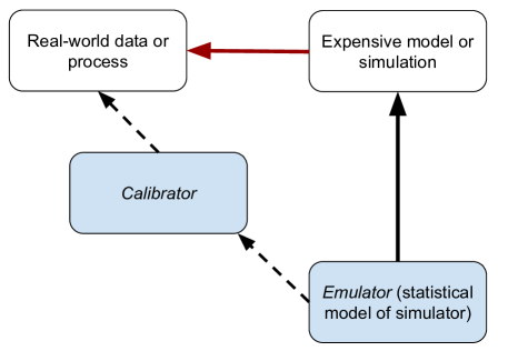
Figure 1: A graphical illustration of the emulation/calibration paradigm. A statistical model approximates a computationally expensive system to enable efficient calibration based on observed data. Our methodology builds both the emulator and calibrator modules through a combination of Gaussian and non-Gaussian state-space methods and Gaussian process regression.

2.1 Gaussian Process Regression

Consider a deterministic dynamical system model that takes as input a $d$-dimensional vector $\bm{x}=(x_{1},\ldots,x_{d})^{\top}$ and outputs a scalar $y(\bm{x})$. To model this unknown relationship, a Gaussian process prior is a flexible choice for the functional form and is written $y(\bm{x})\sim\mathcal{GP}\big{(}\mu,\sigma^{2}{C}(\cdot;\bm{\beta})\big{)}$, where $\mu$, $\sigma^{2}$, $C(\cdot;\bm{\beta})$, and $\bm{\beta}$ are the mean, variance, correlation function, and hyperparameters, respectively. It is often convenient to assume a squared exponential correlation function, which we assume for the rest of this article. This correlation function takes the following form,

$${C}(\bm{x},\bm{x}^{\prime};\bm{\beta})=\exp\big{(}-\sum_{i=1}^{d}\beta_{i}(\bm{x}_{i}-\bm{x}^{\prime}_{i})^{2}\big{)},$$ (1)

where the range parameter $\beta_{i}$ controls the decay of correlation along the $i$-th dimension of $\bm{\beta}$. If $\mathcal{X}=\{\bm{x}_{1},\bm{x}_{2},\ldots,\bm{x}_{N}\}$ are a collection of inputs, then the predictive distribution for a new input $\bm{x}^{*}$ in effect “learns” the functional output for the new input. Standard conditioning identities result in a Gaussian predictive distribution $y(\bm{x}^{*})\mid\bm{y}(\mathcal{X})\sim\mathcal{N}(\bar{\mu}(\bm{x}^{*}),\bar{\sigma}^{2}(\bm{x}^{*}))$ with mean $\bar{\mu}(\bm{x}^{*})=\mu+\bm{r}^{\top}\bm{V}^{-1}(\bm{y}(\mathcal{X})-\mu\bm{1}_{n})$ and variance $\bar{\sigma}^{2}(\bm{x}^{*})=\sigma^{2}-\bm{r}^{\top}\bm{V}^{-1}\bm{r}/\sigma^{2}$, where $\bm{r}=\big{(}C(\bm{x}_{1},\bm{x}^{*};\bm{\beta}),\ldots,C(\bm{x}_{N},\bm{x}^{*};\bm{\beta})\big{)}^{\top}$ is $N\times 1$ and $\bm{V}$ is $N\times N$ with $(i,j)$-th element $C(\bm{x}_{i},\bm{x}_{j};\bm{\beta})$ for pairs of inputs in $\mathcal{X}$. These predictive equations imply the Gaussian process interpolates at the training design points as the variance shrinks to zero.

2.2 Bayesian State-Space Models

Bayesian state-space models (SSMs) – also known as Bayesian dynamic models – are a rich class of non-stationary time series models with a large literature on applied modeling (West and Harrison, 1997; Petris et al., 2009). There are three areas of interest when considering dynamic models: filtering, smoothing, and forecasting. Filtering refers to inference on the current latent state conditional on all current and past data. The most famous example of filtering is the Kalman filter (Kalman, 1960), provably optimal for inference in linear dynamical systems. Smoothing refers to retrodictive inference on the latent process conditional on the entire observed data. Finally, forecasting refers to prediction of the hidden state at any time point beyond the current observation. These ideas are important when building an efficient sampling routine for our model.

Figure 2: DAG representing dynamical evolution of latent parameters and the connection to observed data. Conditional dependencies on hyperparameters are suppressed. Notice both the latent mean and variance are time-varying.

We build from the following general structure of the state-space model,

$$\begin{split}\bm{y}_{t}&=\bm{F}_{t}\bm{\theta}_{t}+\bm{\varepsilon}_{t},\quad\bm{\varepsilon}_{t}\stackrel{{\scriptstyle\text{ind.}}}{{\sim}}\mathcal{N}_{N}(0,v_{t}\bm{V}(\bm{\beta}))\\ \bm{\theta}_{t}&=\bm{G}_{t}\bm{\theta}_{t-1}+\bm{\tau}_{t},\quad\bm{\tau}_{t}\stackrel{{\scriptstyle\text{ind.}}}{{\sim}}\mathcal{N}_{p}(0,v_{t}\bm{W}(\bm{\psi}))\\ v_{t}^{-1}&=\dfrac{\gamma_{t}}{\omega}v_{t-1}^{-1},\quad\gamma_{t}\stackrel{{\scriptstyle\text{ind.}}}{{\sim}}\mathcal{B}(\omega n_{t-1},(1-\omega)n_{t-1}),\end{split}$$ (2)

where $\bm{F}_{t}$ and $\bm{G}_{t}$ are matrices of order $N\times p$ and $p\times p$, respectively. The $N\times N$ and $p\times p$ correlation matrices $\bm{V}$ and $\bm{W}$ are parameterized by $\bm{\beta}$ and $\bm{\psi}$, which will later connect to hyperparameters of Gaussian process innovations. In contrast to standard Gaussian state-space models, we allow both the latent state $\bm{\theta}_{t}$ and $v_{t}$ to obey Markovian dynamics, implying the directed acyclic graph (DAG) of Figure 2. Notice the Gaussian evolution specified for $\bm{\theta}_{t}$ and the non-Gaussian state-space structure of $v_{t}$; see (Gamerman et al., 2013) for a discussion of a broad class of such non-Gaussian models with analytic filtering expressions. In (2), a discount learning rate $\omega\in(0,1]$ is useful for regulating the time-varying dynamics for $v_{t}$ by controlling the magnitude of the $\gamma_{t}$ random variates. The distribution of $\gamma_{t}$ will be discussed later but is necessary to preserve the analytic form of the filtering and smoothing expressions. It may be viewed as a random multiplicative shock with expected value $\mathbb{E}[\gamma_{t}/\omega]=1$. In this way, $\omega$ may also be interpreted as the relative learning rate or stability over time whereby $\omega=1$ is a completely static variance model (West and Harrison, 1997). The learning rate is commonly tuned using predictive criteria, maximization of the log-likelihood, or cross validation. We briefly expand in Appendix 5.2 on this non-Gaussian state-space model for the precision. It should be emphasized this Markov process on the precision holds for any $n_{t}$ and $d_{t}$, but the form of these hyperparameters will be explicitly calculated in the filtering distributions and smoothing distributions. For now, this suffices to build the entire joint prior distribution. To complete the prior specification of the model given starting values $\bm{m}_{0}$, $\bm{M}_{0}$, $n_{0}$, and $d_{0}$, we write the conjugate joint prior as,

$$p(\bm{\theta}_{0},v_{0}^{-1},\bm{\theta}_{1},v_{1}^{-1},\ldots,\bm{\theta}_{T},v_{T}^{-1})=\mathcal{NG}(\bm{\theta}_{0},v_{0}^{-1}\mid\bm{m}_{0},\bm{M}_{0},n_{0},d_{0})\\ \times\prod_{t=1}^{T}\mbox{Scaled-}{\cal B}(v_{t}^{-1}\mid\omega,v_{t-1}^{-1})\times\mathcal{N}\left(\bm{\theta}_{t}\mid\bm{G}_{t}\bm{\theta}_{t-1},v_{t}\bm{W}(\bm{\psi})\right),$$ (3)

where $\mbox{Scaled-}{\cal B}(v_{t}^{-1}\mid\omega,v_{t-1}^{-1})$ is the density corresponding to the conditional distribution of $v_{t}^{-1}$ given $v_{t-1}^{-1}$ in (2). Hence, the ensuing filtering operations of Algorithm 4 remain within the conjugate Normal-Gamma family and easily computed. It is also possible to introduce a second discount factor to specify time-varying but deterministic dynamics for $\bm{W}(\bm{\psi})$ (Farah et al., 2014), but we forego this approach to let $\bm{W}(\bm{\psi})$ capture associations across space through another Gaussian spatial process. This implies the joint posterior of interest is

$$\begin{split}p(v_{0:T},\bm{\theta}_{0:T},\bm{\beta},\bm{\psi}\mid\bm{y}_{1:T})&\propto p(\bm{\beta},\bm{\psi})\times\mathcal{NG}\left(\bm{\theta}_{0},v_{0}^{-1}\mid\bm{m}_{0},\bm{M}_{0},n_{0},d_{0}\right)\\ &\times\mbox{Scaled-}{\cal B}(v_{t}^{-1}\mid\omega,v_{t-1}^{-1})\times\mathcal{N}\left(\bm{\theta}_{t}\mid\bm{G}_{t}\bm{\theta}_{t-1},v_{t}\bm{W}(\bm{\psi})\right)\\ &\hskip 14.22636pt\times\prod_{t=1}^{T}\mathcal{N}\left(\bm{y}_{t}\mid\bm{F}_{t}\bm{\theta}_{t},v_{t}\bm{V}(\bm{\beta})\right).\end{split}$$ (4)

We conclude this section with discussion on the computational efficiency arising through the latent Markov process $\bm{\theta}_{t}$ and precision $v_{t}^{-1}$. This Markov structure enables efficient recursive computing of the full conditionals required for Markov Chain Monte Carlo (MCMC) sampling using filtering and smoothing theory. This recursive computing strategy is known as the forward-filter-backward-sampling (FFBS) algorithm (Carter and Kohn, 1994; Frühwirth-Schnatter, 2006). In essence, this blocked Gibbs sampler relies on the Kalman filter for the forward pass of the algorithm, obtaining the distributional moments required to start the backward pass. In other words, the FFBS algorithm first applies the Kalman filter of Algorithm 4 before initializing the backward sampling through the Kalman or Rauch–Tung–Striebel smoother (Särkkä, 2013) of Algorithm 5. The FFBS algorithm combines the forward and backward steps to build an efficient blocked Gibbs sampler that makes draws from the full latent trajectory $v_{0:T},\bm{\theta}_{0:T}|\bm{y}_{1:T}$ in entirety before proceeding with further parameter updates. This results in much faster convergence and lower autocorrelations in the posterior samples than standard Gibbs routines (Carter and Kohn, 1994; Scott, 2002). The computations necessary for backward sampling of the latent state are well-established (West and Harrison, 1997; Petris et al., 2009), while smoothing expressions for the precision are calculated in the Appendix, as these are less standard. The FFBS algorithm for inferring latent parameters conditional upon $\bm{\beta}$ and $\bm{\psi}$ in model (2) is described below in Algorithm 1.

Algorithm 1 Forward-filter-backward-sample algorithm

1:Input: Data $\bm{y}_{1:T}$ and Kalman filter starting values $n_{0}$, $d_{0}$, $\bm{m}_{0}$, $\bm{M}_{0}$

2:Input: Observation and state transition matrices $\bm{F}_{1:T}$ and $\bm{G}_{1:T}$

3:Input: Correlation matrices $\bm{V}$ and $\bm{W}$

4:Output: Sample from posterior $p(v_{0:T},\bm{\theta}_{0:T}|\bm{y}_{1:T})$

5:function FFBS($\bm{y}_{1:T},n_{0},d_{0},\bm{m}_{0},\bm{M}_{0},\bm{F}_{1:T},\bm{G}_{1:T},\bm{V},\bm{W}$)

6:     $\{n_{t}^{*},d_{t}^{*},\bm{a}_{t},\bm{A}_{t},\bm{m}_{t},\bm{M}_{t}\}_{t=0}^{T}\leftarrow\texttt{Filter}(\bm{y}_{1:T},n_{0},d_{0},\bm{m}_{0},\bm{M}_{0},\bm{G}_{1:T},\bm{F}_{1:T},\bm{V},\bm{W}$)

7:     $\{v_{t},\bm{\theta}_{t}\}_{t=0}^{T}\leftarrow\texttt{BackwardSample}(\{n_{t}^{*},d_{t}^{*},\bm{a}_{t},\bm{A}_{t},\bm{m}_{t},\bm{M}_{t},\bm{G}_{t}\}_{t=0}^{T}$)

8:     return $\{v_{t},\bm{\theta}_{t}\}_{t=0}^{T}$ $\triangleright$ Return sample from $p(\bm{\theta}_{0:T},v_{0:T}|\bm{y}_{1:T})$

9:end function

2.3 Dynamic Spatiotemporal Emulation

We refer to our emulator model as SSGP to emphasize a state-space model driven throughout space and time by Gaussian process innovations. By way of notation, define the following:

• Let $\mathcal{X}=\{\bm{x}_{1},\ldots,\bm{x}_{N}\}$ be a set of $N$ mechanistic system inputs, where each $\bm{x}_{i}$ is a $d$-dimensional vector. Let $\mathcal{S}=\{\bm{s}_{1},\ldots,\bm{s}_{S}\}$ denote the set of observed spatial locations.

• At spatial location $\bm{s}$ at time $t$, collect the outputs for each simulation setting as the $N$-dimensional vector $\bm{y}_{t}(\bm{s})=(y_{t}(\bm{s},\bm{x}_{1}),\ldots y_{t}(\bm{s},\bm{x}_{N}))^{\top}.$ Define the field observations gathered over space as vector $\bm{z}_{t}=(z_{t}(\bm{s}_{1}),\ldots,z_{t}(\bm{s}_{S}))^{\top}$

• Write the latent process at time $t$ as a $pS\times 1$ vector $\bm{\theta}_{t}=(\bm{\theta}_{t}(\bm{s}_{1}),\ldots,\bm{\theta}_{t}(\bm{s}_{S}))^{\top}$. The correlation function over the dynamical system parameter input space is $C(\cdot;\bm{\beta})$ and the cross-correlation function over space is $\bm{K}(\cdot;\bm{\psi})$.

Combing Sections 2.1 and 2.2 inspires the spatiotemporal emulator model of

$$\begin{split}{y}_{t}(\bm{s},\bm{x})&=\bm{f}_{t}(\bm{s},\bm{x})^{\top}\bm{\theta}_{t}(\bm{s})+{\varepsilon}_{t}(\bm{x}),\quad{\varepsilon}_{t}(\bm{x})\stackrel{{\scriptstyle\text{ind.}}}{{\sim}}\mathcal{GP}(0,v_{t}C(\cdot;\bm{\beta}))\\ \bm{\theta}_{t}(\bm{s})&=\bm{G}_{t}(\bm{s})\bm{\theta}_{t-1}(\bm{s})+\bm{\tau}_{t}(\bm{s}),\quad\bm{\tau}_{t}(\bm{s})\stackrel{{\scriptstyle\text{ind.}}}{{\sim}}\mathcal{GP}(0,v_{t}\bm{K}(\cdot;\bm{\psi}))\\ v_{t}^{-1}&=\dfrac{\gamma_{t}}{\omega}v_{t-1}^{-1},\quad\gamma_{t}\stackrel{{\scriptstyle\text{ind.}}}{{\sim}}\mathcal{B}(\omega n_{t-1},(1-\omega)n_{t-1}),\end{split}$$ (5)

where $\bm{f}_{t}(\bm{s},\bm{x})$ is $N\times 1$ and contains the transition terms for the observation equation, while $\bm{G}_{t}(\bm{s})$ is the latent state transition matrix. For example, a simple specification for $\bm{f}$ is an autoregressive order $p$ transition structure at computer input $\bm{x}$ such that $\bm{f}_{t}(\bm{s},\bm{x})=(y_{t-1}(\bm{s},\bm{x}),\ldots,y_{t-p}(\bm{s},\bm{x}))^{\top}$. We take the correlation function $C(\cdot;\bm{\beta})$ as squared exponential, while a convenient parameterization of a valid cross-correlation function for $\bm{K}(\cdot;\bm{\psi})$ is to consider a $p\times p$ positive definite matrix $\bm{T}$ such that

$$\bm{K}\left(\bm{s},\bm{s}^{\prime};\bm{\psi}\right)=C\left(\bm{s},\bm{s}^{\prime};\bm{\Omega}\right)\cdot\bm{T},$$ (6)

where $\bm{\psi}=\left\{\bm{\Omega},h(\bm{T})\right\}$, and $C(\cdot;\bm{\Omega})$ is another squared exponential. Here the $p\times p$ matrix $\bm{T}$ is the covariance for specific $\bm{\theta}_{t}(\bm{s})$, while $C(\cdot;\bm{\Omega})$ models correlation across the spatial locations. We expand on the form of $\bm{K}$ by considering a realization of the process on some set of spatial locations, such that applying $\bm{K}$ results in a matrix $\bm{W}(\bm{\psi})=\bm{H}\otimes\bm{T}$ where $(\bm{H})_{ij}=C\left(\bm{s}_{i},\bm{s}_{j};\bm{\Omega}\right)$ and $\otimes$ denotes the Kronecker product. The matrix $\bm{W}(\bm{\psi})$ is convenient to work with since $\left|\bm{W}(\bm{\psi})\right|=|\bm{H}|^{S}|\bm{T}|^{p}$ and $\bm{W}(\bm{\psi})^{-1}=\bm{H}^{-1}\otimes\bm{T}^{-1}$. A parsimonious approach is to consider the parameters comprising $\bm{\theta}(\bm{s})$ as independent, in which case $\bm{T}=\bm{I}$. A richer model specification involves an inverse Wishart prior for $\bm{T}$, so the full conditional distribution $p(\bm{T}\mid\cdot)$ remains inverse Wishart. Unfortunately, $\bm{T}$ (and hence $\bm{W}(\bm{\psi})$) is not identifiable due to the scaling factor $v_{t}$ in (5). However, to each covariance matrix $\bm{T}$, there corresponds a unique correlation matrix obtained by the function

$$h(\bm{T})=\left(\sigma_{ij}/\sqrt{\sigma_{i}^{2}\sigma_{j}^{2}}\right)_{ij},$$ (7)

where $\sigma_{ij}$ is the $(i,j)$-th element of $\bm{T}$. Since the value of $\bm{W}(\bm{\psi})=\bm{H}\otimes h(\bm{T})$ is identifiable, one estimation approach is to reparameterize the model in terms of this non-identifiable covariance matrix $\bm{T}$, while focusing posterior inference on the identifiable correlation matrix $\bm{W}(\bm{\psi})$ after making the transformation $h(\bm{T})$. The addition of a non-identifiable parameter within Bayesian models to simplify calculations is well-established as parameter expansion (Liu and Wu, 1999; Gelman, 2004). The sampling is then an additional step in Algorithm 2: set $SS=\sum_{t=1}^{T}\sum_{i=1}^{S}(\bm{\theta}_{t}(\bm{s}_{i})-\bm{G}_{t}(\bm{s}_{i})\bm{\theta}_{t-1}(\bm{s}_{i}))(\bm{\theta}_{t}(\bm{s}_{i})-\bm{G}_{t}(\bm{s}_{i})\bm{\theta}_{t-1}(\bm{s}_{i}))^{\top}$ and then draw $\bm{T}^{-1}\sim\mathcal{W}\left(\nu_{0}+T/2,\bm{T}_{0}+SS/2\right)$.

Consider a multivariate vector autogressive state-space model whereby we form the $N\times N$ correlation matrix $\bm{V}$ and write the autoregressive matrix of dimension $N\times p$ at spatial location $\bm{s}$ as

$$\bm{F}_{t}(\bm{s})=\begin{bmatrix}y_{t-1}(\bm{s},\bm{x}_{1})&\cdots&y_{t-p}(\bm{s},\bm{x}_{1})\\ \vdots&\ddots&\vdots\\ y_{t-1}(\bm{s},\bm{x}_{N})&\cdots&y_{t-p}(\bm{s},\bm{x}_{N})\end{bmatrix}.$$

Given the observed spatial locations $\mathcal{S}=\{\bm{s}_{1},\ldots,\bm{s}_{S}\}$, the $pS\times pS$ correlation matrix is $\bm{W}(\bm{\psi})$, so the realized computer emulation model is

$$\begin{split}\bm{y}_{t}(\bm{s})&=\bm{F}_{t}(\bm{s})\bm{\theta}_{t}(\bm{s})+\bm{\varepsilon}_{t}(\bm{s}),\quad\bm{\varepsilon}_{t}(\bm{s})\stackrel{{\scriptstyle\text{ind.}}}{{\sim}}\mathcal{N}(0,v_{t}\bm{V}(\bm{\beta}))\\ \bm{\theta}_{t}&={\bm{G}_{t}}\bm{\theta}_{t-1}+\bm{\tau}_{t},\quad\bm{\tau}_{t}\stackrel{{\scriptstyle\text{ind.}}}{{\sim}}\mathcal{N}(0,v_{t}\bm{W}(\bm{\psi}))\\ v_{t}^{-1}&=\dfrac{\gamma_{t}}{\omega}v_{t-1}^{-1},\quad\gamma_{t}\stackrel{{\scriptstyle\text{ind.}}}{{\sim}}\mathcal{B}(\omega n_{t-1},(1-\omega)n_{t-1}),\end{split}$$ (8)

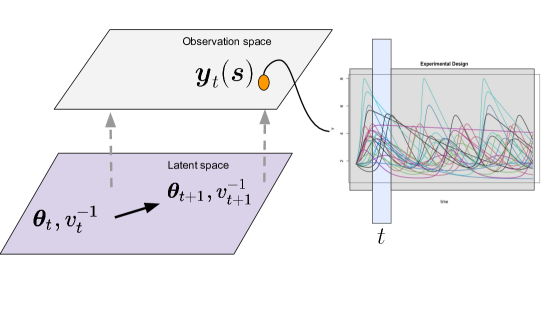
Figure 3: A pictorial representation of the spatiotemporal state-space Gaussian process surrogate model. On the left, the spatiotemporal dynamics are modeled in the latent space. Each spatial location $\bm{y}_{t}(\bm{s})$ in the observation space contains a collection of curves generated through differing computer input settings, shown on the right. At each time $t$, a Gaussian process models the computer design space generating the differing curves.

After introducing priors $p(\bm{\beta},\bm{\gamma},\bm{\psi})$ and $\mathcal{NG}\left(\bm{\theta}_{0},v_{0}^{-1}|\bm{m}_{0},\bm{M}_{0},n_{0},d_{0}\right)$, the posterior is

$$\begin{split}p(v_{0:T},\bm{\theta}_{0:T},\bm{\beta},\bm{\psi}|\bm{y}_{1:T})&\propto p(\bm{\beta},\bm{\psi})\mathcal{NG}\left(\bm{\theta}_{0},v_{0}^{-1}\mid\bm{m}_{0},\bm{M}_{0},n_{0},d_{0}\right)\\ &\times\mbox{Scaled-}{\cal B}(v_{t}^{-1}\mid\omega,v_{t-1}^{-1})\times\mathcal{N}\left(\bm{\theta}_{t}\mid\bm{G}_{t}\bm{\theta}_{t-1},v_{t}\bm{W}(\bm{\psi})\right)\\ &\hskip 14.22636pt\times\prod_{t=1}^{T}\prod_{i=1}^{S}\mathcal{N}\left(\bm{y}_{t}(\bm{s}_{i})\mid\bm{F}_{t}(\bm{s}_{i})\bm{\theta}_{t}(\bm{s}_{i}),v_{t}\bm{V}(\bm{\beta})\right),\end{split}$$ (9)

where the prior hyperparameters arise from the Kalman filter Algorithm 4. Draws from the posterior (9) enable forecasting computer model output for unknown input $\bm{\eta}$ using the emulator’s predictive distribution. The predictive distribution of $y_{t}^{*}(\bm{s},\bm{\eta})$, which is the unknown output at $\bm{s}$ corresponding to input $\bm{\eta}$, is derived from the joint distribution,

$$\small\left[\begin{matrix}y_{t}^{*}(\bm{s},\bm{\eta})\\ \bm{y}_{t}(\bm{s})\end{matrix}\Big{|}\bm{f}_{t}(\bm{s},\bm{\eta}),\bm{F}_{t}(\bm{s}),\bm{\eta},v_{t},\bm{\theta}_{t},\bm{\beta}\right]\sim\mathcal{N}\left(\begin{bmatrix}\bm{f}_{t}(\bm{s},\bm{\eta})^{\top}\bm{\theta}_{t}(\bm{s})\vspace{1mm}\\ \bm{F}_{t}(\bm{s})\bm{\theta}_{t}(\bm{s})\end{bmatrix},\begin{bmatrix}v_{t}&\bm{r}(\bm{\eta})^{\top}\\ \bm{r}(\bm{\eta})&v_{t}\bm{V}(\bm{\beta})\end{bmatrix}\right),$$ (10)

with $\bm{r}(\bm{\eta})=\left(C(\bm{x}_{1},\bm{\eta};\bm{\beta}),\ldots,C(\bm{x}_{N},\bm{\eta};\bm{\beta})\right)^{\top}$. Like in Section 2.1, the emulator predictive density at input $\bm{\eta}$ is given after conditioning (10) so that $y_{t}^{*}(\bm{s},\bm{\eta})|\bm{\eta},v_{t},\bm{\theta}_{t},\bm{\beta}\sim\mathcal{N}(\widetilde{\mu}_{t}(\bm{s},\bm{\eta}),\widetilde{\sigma}_{t}^{2}(\bm{s},\bm{\eta})),$ where

$$\begin{split}\widetilde{\mu}_{t}(\bm{s},\bm{\eta})&=\bm{f}_{t}(\bm{s},\bm{\eta})^{\top}\bm{\theta}_{t}(\bm{s})+\bm{r}(\bm{\eta})^{\top}\bm{V}(\bm{\beta})^{-1}\big{(}\bm{y}_{t}(\bm{s})-\bm{F}_{t}(\bm{s})\bm{\theta}_{t}(\bm{s})\big{)}\\ \widetilde{\sigma}_{t}^{2}(\bm{s},\bm{\eta})&=v_{t}(1-\bm{r}(\bm{\eta})^{\top}\bm{V}(\bm{\beta})^{-1}\bm{r}(\bm{\eta})).\end{split}$$ (11)

Additionally, we can interpolate the latent state $\bm{\theta}_{t}(\bm{s}^{*})$ at an arbitrary spatial location $\bm{s}^{*}$ using the posterior samples from (9). To be precise, we have $\bm{\theta}_{t}(\bm{s}^{*})|\bm{\theta}_{t-1}(\bm{s}^{*}),\bm{\theta}_{t-1:t},v_{t},\bm{\psi}\sim\mathcal{N}_{p}(\bm{\lambda}_{t}(\bm{s}^{*}),\bm{\Lambda}_{t}(\bm{s}^{*}))$ where

$$\begin{split}\bm{\lambda}_{t}(\bm{s}^{*})&=\bm{G}_{t}(\bm{s}^{*})\bm{\theta}_{t-1}(\bm{s}^{*})+\bm{k}(\bm{s}^{*})^{\top}\bm{W}(\bm{\psi})^{-1}(\bm{\theta}_{t}-\bm{G}_{t}\bm{\theta}_{t-1})\\ \bm{\Lambda}_{t}(\bm{s}^{*})&=v_{t}\bm{K}(\bm{s}^{*},\bm{s}^{*};\bm{\psi})-v_{t}\bm{k}(\bm{s}^{*})^{\top}\bm{W}(\bm{\psi})^{-1}\bm{k}(\bm{s}^{*}),\end{split}$$ (12)

where the matrix $\bm{k}(\bm{s}^{*})^{\top}=\left[\bm{K}(\bm{s}_{1},\bm{s}^{*};\bm{\psi}):\dots:\bm{K}(\bm{s}_{S},\bm{s}^{*};\bm{\psi})\right]$ is $p\times pS$. This general idea has computational implications for dimension reduction (see Section 2.5). We sample from the posterior distribution $p(\{\bm{\theta}_{t}(\bm{s}^{*})\}\mid\bm{y}_{1:T})$ by drawing, sequentially for $t=1:T$, $\bm{\theta}_{t}(\bm{s}^{\ast})$ from $\mathcal{N}_{p}(\bm{\lambda}_{t}(\bm{s}^{*}),\bm{\Lambda}_{t}(\bm{s}^{*}))$, where $\bm{\lambda}_{t}(\bm{s}^{*})$ and $\bm{\Lambda}_{t}(\bm{s}^{*})$ are evaluated using the sampled values of the parameters from the posterior distribution in (9). Repeating this for each sampled value of the parameters results in the posterior samples for $\bm{\theta}_{t}({\bm{s}^{\ast}})$. We can then predict $\bm{Y}_{t}(\bm{s}^{\ast})$ with full uncertainty quantification by drawing samples from the posterior predictive distribution $p(\bm{Y}_{t}(\bm{s}^{\ast})\mid\bm{y}_{1:T})$ by sampling one value of $\bm{Y}_{t}(\bm{s}^{\ast})$ from ${\cal N}(\bm{F}_{t}(\bm{s}^{\ast})\bm{\theta}_{t}(\bm{s}^{\ast}),v_{t}\bm{V}(\bm{\beta}))$ for each drawn value of $\bm{\theta}_{t}(\bm{s}^{\ast})$, $v_{t}$ and $\bm{\beta}$ from their posterior distribution in (9). The complete posterior sampling algorithm for dynamic emulation is given in Algorithm 2.

Algorithm 2 Sampler for emulation

1:Given: Data $\bm{y}_{1:T}$, discount factor $\omega$, and tuning parameters $\epsilon_{1},\epsilon_{2}$

2:Initialize: Gaussian process hyperparameters $\bm{\beta}^{(0)}$, $\bm{\psi}^{(0)}$

3:Initialize: Kalman filter starting values $n_{0}$, $d_{0}$, $\bm{m}_{0}$, $\bm{M}_{0}$

4:Output: posterior samples from $p(v_{0:T},\bm{\theta}_{0:T},\bm{\beta},\bm{\psi}|\bm{y}_{1:T})$

5:for $i=1$ to $No.\ samples$ do

6:     $\{\bm{\beta}^{(i)},\bm{\psi}^{(i)},v_{0:T}^{(i)},\bm{\theta}_{0:T}^{(i)}\}\leftarrow\texttt{updateEmulator}(\bm{y}_{1:T},\bm{\beta}^{(i-1)},\bm{\psi}^{(i-1)},\bm{\theta}_{0:T}^{(i-1)},v_{0:T}^{(i-1)})$

7:end for

8:function updateEmulator($\bm{y}_{1:T},\bm{\beta},\bm{\theta},\bm{\theta}_{0:T},v_{0:T}$)

9:     $\bm{\psi}^{*}\leftarrow\exp(\log(\bm{\psi})+\mathcal{N}(0,\epsilon_{1}^{2}\bm{I}))$ $\triangleright$ Propose spatial process hyperparameters

10:     Compute Jacobian $J\left(\bm{\psi}\right)=\prod_{i=1}^{d}\bm{\psi}_{i}^{-1}$

11:     Compute correlation matrix $\bm{W}(\bm{\psi})$ through $\bm{K}(\cdot;\bm{\psi})$ and $\bm{W}(\bm{\psi}^{*})$ through $\bm{K}(\cdot;\bm{\psi}^{*})$

12:     With probability $\max\left\{\dfrac{\prod_{t}\mathcal{N}(\bm{\theta}_{t}|\bm{G}_{t}\bm{\theta}_{t-1},\bm{v}_{t}\bm{W}(\bm{\psi}^{*}))p(\bm{\psi}^{*})\mathcal{J}(\bm{\psi})}{\prod_{t}\mathcal{N}(\bm{\theta}_{t}|\bm{G}_{t}\bm{\theta}_{t-1},\bm{v}_{t}\bm{W}(\bm{\psi}))p(\bm{\psi})\mathcal{J}(\bm{\psi}^{*})},1\right\}$, $\bm{\psi}\leftarrow\bm{\psi}^{*}$

13:     $\bm{\beta}^{*}\leftarrow\exp(\log(\bm{\beta})+\mathcal{N}(0,\epsilon_{2}^{2}\bm{I}))$ $\triangleright$ Propose computer process hyperparameters

14:     Compute correlation matrix $\bm{V}(\bm{\beta})$ through $C(\cdot;\bm{\beta})$ and $\bm{V}^{*}(\bm{\beta}^{*})$ through $C(\cdot;\bm{\beta}^{*})$

15:     # Using the likelihood from (9) and Jacobian $J\left(\bm{\beta}\right)=\prod_{i=1}^{d}\bm{\beta}_{i}^{-1}$

16:     With probability $\max\left\{\dfrac{\mathcal{L}(\bm{\beta}^{*})p(\bm{\beta}^{*})\mathcal{J}(\bm{\beta})}{\mathcal{L}(\bm{\beta})p(\bm{\beta})\mathcal{J}(\bm{\beta}^{*})},1\right\},\bm{\beta}\leftarrow\bm{\beta}^{*}$

17:     $\{v_{t}^{*},\bm{\theta}_{t}^{*}\}_{t=0}^{T}\leftarrow\texttt{FFBS}(\bm{y}_{1:T},n_{0},d_{0},\bm{m}_{0},\bm{M}_{0},\bm{G}_{1:T},\bm{F}_{1:T},\bm{V}(\bm{\beta}),\bm{W}(\bm{\psi}))$$\triangleright$ Algorithm 1

18:     return $\{\bm{\beta},\bm{\psi},v_{0:T}^{*},\bm{\theta}_{0:T}^{*}\}$

19:end function

2.4 Calibration with Model Bias

The above emulator is now used to solve the spatiotemporal calibration problem. Often mathematical or computational models may not adequately describe observed field data over all spatial locations and time points. Hence, we include a spatiotemporally-varying misspecification term that captures bias between the observed field data and emulator in the calibration process. Our state-space calibration model with dynamic bias correction $\bm{u}$ is

$$\begin{split}z_{t}(\bm{s})&=y_{t}^{*}(\bm{s},\bm{\eta})+u_{t}(\bm{s})+\varepsilon_{t}^{z}(\bm{s}),\quad\varepsilon_{t}^{z}(\bm{s})\stackrel{{\scriptstyle\text{ind.}}}{{\sim}}\mathcal{N}(0,\nu_{t})\\ {u_{t}(\bm{s})}&=u_{t-1}(\bm{s})+\omega_{t}(\bm{s}),\quad\omega_{t}(\bm{s})\stackrel{{\scriptstyle\text{ind.}}}{{\sim}}\mathcal{GP}(0,\nu_{t}C(\cdot;\bm{\rho}))\\ \nu_{t}^{-1}&=\dfrac{\gamma_{t}}{b}\nu_{t-1}^{-1},\quad\gamma_{t}\stackrel{{\scriptstyle\text{ind.}}}{{\sim}}\mathcal{B}(bn_{t-1},(1-b)n_{t-1}),\end{split}$$ (13)

where $y_{t}^{*}(\bm{s},\bm{\eta})$ denotes the emulator prediction. Let $\bm{U}(\bm{\rho})$ be the $S\times S$ correlation matrix built through $C(\cdot;\bm{\rho})$. After introducing priors $\mathcal{U}(\bm{\eta}|0,1)\text{ and }\mathcal{NG}(\bm{u}_{0},\nu_{0}^{-1}|\bm{m}_{0},\bm{M}_{0},n_{0},d_{0})$, conditioning on the emulator of the previous section yields the posterior distribution

$$\begin{split}&\propto p(\bm{\rho})\mathcal{U}(\bm{\eta}|0,1)\mathcal{NG}(\bm{u}_{0},\nu_{0}^{-1}|\bm{m}_{0},\bm{M}_{0},n_{0},d_{0})\\ &\hskip 14.22636pt\times\mbox{Scaled-}{\cal B}(\nu_{t}^{-1}\mid b,\nu_{t-1}^{-1})\times\mathcal{N}\left(\bm{u}_{t}\mid\bm{u}_{t-1},\nu_{t}\bm{U}(\bm{\rho})\right)\\ &\hskip 14.22636pt\times\prod_{t=1}^{T}\prod_{i=1}^{S}\mathcal{N}\left(z_{t}(\bm{s}_{i})|\widetilde{\mu}_{t}(\bm{\eta},\bm{s}_{i}),\widetilde{\sigma}_{t}(\bm{\eta},\bm{s}_{i})\right),\end{split}$$ (14)

where $\widetilde{\mu}_{t}(\bm{\eta},\bm{s})$ and $\widetilde{\sigma_{t}}(\bm{\eta},\bm{s})$ are defined as

$$\begin{split}\widetilde{\mu}_{t}(\bm{s},\bm{\eta})&=\bm{f}_{t}(\bm{s},\bm{\eta})^{\top}\bm{\theta}_{t}(\bm{s})+u_{t}(\bm{s})+\bm{r}(\bm{\eta})^{\top}\bm{V}(\bm{\beta})^{-1}\left(\bm{y}_{t}(\bm{s})-\bm{F}_{t}(\bm{s})\bm{\theta}_{t}(\bm{s})\right)\\ \widetilde{\sigma}_{t}^{2}(\bm{s},\bm{\eta})&=\nu_{t}+v_{t}\left(1-\bm{r}(\bm{\eta})^{\top}\bm{V}(\bm{\beta})^{-1}\bm{r}(\bm{\eta})\right).\end{split}$$ (15)

The primary interest often lies in sampling from the marginal posterior distribution

$$\begin{split}p(\bm{\eta},\bm{\rho},\nu_{0:T},\bm{u}_{0:T}|\bm{z}_{1:T},\bm{y}_{1:T})&=\int p(\bm{\eta},\bm{\rho},\nu_{0:T},v_{0:T},\bm{\theta}_{0:T},\bm{\beta},\bm{\psi}|\bm{z}_{1:T},\bm{y}_{1:T})dv_{0:T}d\bm{\theta}_{0:T}d\bm{\beta}d\bm{\psi}\\ &=\int p(\bm{\eta},\bm{\rho},\nu_{0:T},\bm{u}_{0:T}\big{|}v_{0:T},\bm{\theta}_{0:T},\bm{\beta},\bm{\psi},\bm{z}_{1:T},\bm{y}_{1:T})\\ &\hskip 28.45274pt\times{\color[rgb]{0,0,0}\underbracket{p(v_{0:T},\bm{\theta}_{0:T},\bm{\beta},\bm{\psi}|\bm{z}_{1:T},\bm{y}_{1:T}}_{\mathclap{\text{Modularize}}}})dv_{0:T}d\bm{\theta}_{0:T}d\bm{\beta}d\bm{\psi},\end{split}$$ (16)

where the emulator parameters have been integrated out. A pragmatic approach to sampling from (16) relies on the posterior in (LABEL:calibrator) and the notion of Bayesian Modularization (Bayarri et al., 2009). Modularization replaces the underlined expression with the lower dimensional distribution $p(v_{0:T},\bm{\theta}_{0:T},\bm{\beta},\bm{\psi}|\bm{y}_{1:T})$, which is readily sampled through FFBS and Metropolis-Hastings steps of Algorithm 1. Once these samples are available, we use Algorithm 3 to sample from (LABEL:calibrator), thus achieving draws from the desired marginal (16). This is justified both computationally and theoretically, as the observed field data should not influence our construction of a statistical emulator. Marginal distribution (16) is thus a principled way to account for emulator uncertainty when calibrating to observed data.

There exists a final opportunity to employ Bayesian modularization to prevent the model discrepancy term $\bm{u}_{t}$ from interfering with the calibration. This additional modularization treats the emulator as an unbiased representation of the field data. After fully sampling calibration parameters, each update of the dynamic bias term conditions upon a draw from the parameter posterior to model the discrepancy between the field data and emulator predictive distribution.

Algorithm 3 Sampler for calibration with computer model bias

1:Given: Field data $\bm{z}_{1:T}$ and tuning parameter $\epsilon_{3}$

2:Initialize: Gaussian process hyperparameters $\bm{\rho}^{(0)}$

3:Execute Algorithm 2 and save MCMC samples $\triangleright$ Modularization step for emulation

4:for $i=1$ to $No.\ samples$ do

5:     $\bm{\zeta}\leftarrow\text{logit}^{-1}\left(\bm{\eta}^{(i-1)}\right)$

6:     $\bm{\eta}^{*}\leftarrow\text{logit}\left(\bm{\zeta}+\mathcal{N}(0,\epsilon_{3}^{2}\bm{I})\right)$ $\triangleright$ Propose calibration parameters

7:     With probability $\max\left\{\dfrac{\mathcal{L}(\bm{\eta}^{*})p(\bm{\eta}^{*})\mathcal{J}(\bm{\eta})}{\mathcal{L}(\bm{\eta})p(\bm{\eta})\mathcal{J}(\bm{\eta}^{*})},1\right\},\bm{\eta}^{(i)}\leftarrow\bm{\eta}^{*}$ $\triangleright$ Using the likelihood (LABEL:calibrator)

8:     Set $\bm{z}_{t}^{*}=(y^{*}_{t}(\bm{s}_{1},\bm{\eta}),\ldots,y^{*}_{t}(\bm{s}_{S},\bm{\eta}))^{\top}$ $\triangleright$ Stack over space in (11)

9:     $\bm{\rho}^{(i)},\nu_{0:T}^{(i)},\bm{u}_{0:T}^{(i)}\leftarrow\texttt{updateDynamicBias}(\bm{z}^{*}_{1:T},\bm{\rho}^{(i-1)},\bm{u}_{0:T}^{(i-1)},\nu_{0:T}^{(i-1)})$

10:end for

11:function updateDynamicBias($\bm{z}_{1:T}^{*},\bm{\rho},\bm{u}_{0:T},\bm{\nu}_{0:T}$)

12:     $\bm{\rho}^{*}\leftarrow\exp(\log(\bm{\rho})+\mathcal{N}(0,\epsilon_{3}^{2}\bm{I}))$ $\triangleright$ Propose bias process hyperparameters

13:     Compute correlation matrix $\bm{U}(\bm{\rho})$ through $C(\cdot;\bm{\rho})$ and $\bm{U}(\bm{\rho}^{*})$ through $C(\cdot;\bm{\rho}^{*})$

14:     # Using the likelihood from (LABEL:calibrator) and Jacobian $J\left(\bm{\rho}\right)=\prod_{i=1}^{d}\bm{\rho}_{i}^{-1}$

15:     With probability $\max\left\{\dfrac{\prod_{t}\mathcal{N}(\bm{u}_{t}|\bm{u}_{t-1},\nu_{t}\bm{U}(\bm{\rho}^{*}))p(\bm{\rho}^{*})\mathcal{J}(\bm{\rho})}{\prod_{t}\mathcal{N}(\bm{u}_{t}|\bm{u}_{t-1},\nu_{t}\bm{U}(\bm{\rho}))p(\bm{\rho})\mathcal{J}(\bm{\rho}^{*})},1\right\}$, $\bm{\rho}\leftarrow\bm{\rho}^{*}$

16:     $\{\nu_{t}^{*},\bm{u}_{t}^{*}\}_{t=0}^{T}\leftarrow\texttt{FFBS}(\bm{z}_{1:T}^{*},n_{0},d_{0},\bm{m}_{0},\bm{M}_{0},-,-,\bm{I},\bm{U}(\bm{\rho}))$ $\triangleright$ Algorithm 1

17:     return $\{\bm{\rho},\nu_{0:T}^{*},\bm{u}_{0:T}^{*}\}$

18:end function

2.5 Strategies for Scalability

This section demonstrates strategies for scaling our framework to the setting of large spatiotemporal computer model learning. The first strategy is purely computational, where we eschew spatial structure for a fully heterogeneous conjugate Bayesian model amenable to embarrassingly parallel computation. An alternative strategy makes use of a rich collection of low rank models to preserve approximate spatial structure.

2.5.1 Seemingly Unrelated Spatiotemporal Models

We first present a scalable emulator inspired from the time series literature on seemingly unrelated time series equations (Zellner and Ando, 2010; Wooldridge, 2002). The assumption of the model is that error terms are independent across observations, but may have cross-equation correlations within observations due to the computer input space. In other words, each spatial location is modeled independently, while each site shares the influence from the computer input space. Using the notation of Section 2.3, the fully heterogeneous emulator with no underlying latent spatial structure is

$$\begin{split}{y}_{t}(\bm{s},\bm{x})&=\bm{f}_{t}(\bm{s},\bm{x})^{\top}\bm{\theta}_{t}(\bm{s})+\bm{\varepsilon}_{t}(\bm{x}),\quad\bm{\varepsilon}_{t}(\bm{x})\stackrel{{\scriptstyle\text{ind.}}}{{\sim}}\mathcal{GP}\left(0,v_{t}(\bm{s})C(\cdot;\bm{\beta})\right)\\ \bm{\theta}_{t}(\bm{s})&=\bm{G}_{t}(\bm{s})\bm{\theta}_{t-1}(\bm{s})+\bm{\tau}_{t}(\bm{s}),\quad\bm{\tau}_{t}(\bm{s})\stackrel{{\scriptstyle\text{ind.}}}{{\sim}}\mathcal{N}\left(0,v_{t}(\bm{s})\bm{W}(\bm{s})\right)\\ v_{t}(\bm{s})^{-1}&=\dfrac{\gamma_{t}(\bm{s})}{\omega}v_{t-1}^{-1}(\bm{s}),\quad\gamma_{t}(\bm{s})\stackrel{{\scriptstyle\text{ind.}}}{{\sim}}\mathcal{B}(\omega n_{t-1}(\bm{s}),(1-\omega)n_{t-1}(\bm{s})),\end{split}$$ (17)

where $\bm{W}(\bm{s})=\text{Corr}(\bm{\theta}_{t}(\bm{s}))$. Such model structure is amenable to embarrassingly parallel computation, where $S$ applications of FFBS run during the MCMC sampling in Algorithm 2. We provide this model implementation in our code as well as the fully spatial version to provide comparison. As this heterogeneous spatial model is a “forest” of 1-dimensional state-space Gaussian process emulators, we make use of the univariate discount factor specification to specify time-varying but deterministic correlation dynamics for $\bm{W}(\bm{s})$ (Liu and West, 2009).

2.5.2 Low Rank Gaussian Processes

To retain the latent spatial structure but facilitate scalable computation, we replace the process $\bm{\theta}_{t}$ with a low-rank approximation such as the Gaussian predictive process (Banerjee et al., 2008; Quiñonero-Candela and Rasmussen, 2005). More precisely, we consider a smaller set of sites in the domain of interest called “knots,” say $\mathcal{S}^{*}=\{\bm{s}_{1}^{*},\ldots,\bm{s}^{*}_{S^{*}}\}$ where $S^{*}\ll S$. Now let $\bm{\tau}_{t}^{*}$ be a realization of $\bm{\tau}_{t}(\bm{s})$ over $\mathcal{S}^{*}$. That is, $\bm{\tau}_{t}^{*}$ is $pS^{*}\times 1$ with entries $\bm{\tau}_{t}(\bm{s}_{i}^{*})$ and $\bm{\tau}_{t}^{*}\sim\mathcal{N}(0,v_{t}{\bm{K}}^{*}(\bm{\psi}))$, where ${\bm{K}}^{*}(\bm{\psi})$ is the associated $pS^{*}\times pS^{*}$ correlation matrix with entries ${\bm{K}}(\bm{s}_{i}^{*},\bm{s}_{j}^{*};\bm{\psi})$. The spatial interpolant that leads to the Kriging estimate at spatial location $\bm{s}_{0}$ is given by

$${\bm{\tau}}(\bm{s}_{0})=\mathbb{E}[\bm{\tau}_{t}(\bm{s}_{0})|\bm{\tau}_{t}^{*}]=\bm{k}(\bm{s}_{0};\bm{\psi})^{\top}{\bm{K}}^{*}(\bm{\psi})^{-1}{\bm{\tau}}_{t}^{*}.$$ (18)

This interpolator defines a spatial process $\widetilde{\bm{\tau}}_{t}(\bm{s})\sim\mathcal{GP}(0,{\bm{K}}^{*}(\cdot;\bm{\psi}))$. The cross-correlation function of this low-rank process takes the form

$${\bm{K}}^{*}(\bm{s},\bm{s}^{\prime};\bm{\psi})=\bm{k}(\bm{s};\bm{\psi})^{\top}{\bm{K}}^{*}(\bm{\psi})^{-1}\bm{k}(\bm{s}^{\prime};\bm{\psi}),$$ (19)

with $\bm{k}(\bm{s};\bm{\psi})^{\top}$ a $p\times pS^{*}$ matrix whose $j$-th column is ${\bm{K}}(\bm{s},\bm{s}_{j}^{*};\bm{\psi})$ for $j\in\{1,\ldots,S^{*}\}$. Replacing $\bm{\tau}_{t}(\bm{s})$ in (5) with $\widetilde{\bm{\tau}}_{t}(\bm{s})+\widetilde{\bm{\varepsilon}}_{t}(\bm{s})$ completes the scalable emulator specification. The term $\widetilde{\bm{\varepsilon}}_{t}(\bm{s})$ is introduced to account for a new source of error with distributional form, $\mathcal{N}_{p}(0,\bm{\Delta}(\bm{s}))$ where $\bm{\Delta}(\bm{s})={\bm{K}}(\bm{s},\bm{s};\bm{\psi})-\bm{k}(\bm{s};\bm{\psi})^{\top}{\bm{K}}^{*}(\bm{\psi})^{-1}\bm{k}(\bm{s};\bm{\psi})$ is diagonal $pS^{*}\times pS^{*}$; see Finley et al. (2012) for discussion of this bias-corrected predictive processes. The additional source of error arises as the conditional expectation projects to a new Hilbert space and induces additional over-smoothing. This projection reduces the computational complexity during sampling from $\mathcal{O}(S^{3})$ to $\mathcal{O}(S^{*3})$. To summarize, the scalable Gaussian predictive process dynamic emulator on knot locations $\mathcal{S}^{*}$ is

$$\begin{split}{y}_{t}(\bm{s},\bm{x})&={\color[rgb]{0,0,0}\bm{f}_{t}(\bm{s},\bm{x})^{\top}}{\bm{\theta}}_{t}(\bm{s})+\varepsilon_{t}(\bm{x}),\ \varepsilon_{t}(\bm{x})\stackrel{{\scriptstyle\text{ind.}}}{{\sim}}\mathcal{GP}(0,v_{t}{C}(\cdot;\bm{\beta}))\\ {\bm{\theta}}_{t}(\bm{s})&={\bm{G}_{t}(\bm{s})\bm{\theta}}_{t-1}(\bm{s})+\widetilde{\bm{\tau}}_{t}(\bm{s}),\ \widetilde{\bm{\tau}}_{t}(\bm{s})\stackrel{{\scriptstyle\text{ind.}}}{{\sim}}\mathcal{GP}(0,v_{t}\bm{K}^{**}(\cdot;\bm{\psi})),\end{split}$$ (20)

where $\bm{K}^{**}(\bm{s},\bm{s}^{\prime};\bm{\psi})=\bm{K}^{*}(\bm{s},\bm{s}^{\prime};\bm{\psi})+\bm{1}(\bm{s}=\bm{s}^{\prime})\bm{\Delta}(\bm{s})$. Sampling from the posterior of (20) is a straightforward modification of Algorithm 2 using the new correlation function $\bm{K}^{**}$. Lastly, we mention knot selection can be an important consideration in applied modeling; see Finley et al. (2009) or (Banerjee et al., 2014, Ch. 12) for various selection criteria. However, in our applied analyses, we found the calibration robust to knot placement.

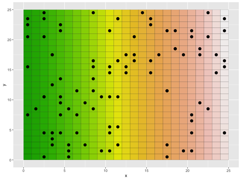
Figure 4: An evolving spatiotemporal system overlaid with a subset of random knot locations, denoted in black, defining a reduced rank Gaussian predictive process.

2.5.3 Massively scalable Gaussian processes

While the Gaussian predictive process and other low rank process formulations (see, e.g., Wikle and Hooten, 2010, for an excellent review of low rank spatial models) can offer effective scalability when the number of locations are in the order of $\sim 10^{4}$, we note a burgeoning literature in scalable Gaussian processes for massive spatiotemporal data with number of locations $\sim 10^{7}+$. Several of these are based upon Vecchia’s approximation (Vecchia, 1988) or graphical models (Datta et al., 2016, 2016b; Katzfuss and Guinness, 2021; Peruzzi et al., 2022) that construct sparsity inducing processes and are often preferred to low rank models as the latter tend to oversmooth at massive scales (also see Banerjee, 2017; Heaton et al., 2019, and references therein for comparisons of different approaches). Different algorithms in Bayesian settings have been explored and compared in Finley et al. (2019). Several of these scalable processes are can seamlessly replace the full Gaussian process or the Gaussian predictive process discussed earlier should there be a need for scalability to massive numbers of spatial locations.

2.6 Model Scoring

For model comparison and scoring purposes, we make use of a criteria based upon the predictive distribution of independently replicated data developed by Gneiting and Raftery (2007). To develop notation for the scoring rule, let ${z}_{t}^{\text{rep}}(\bm{s}_{j})$ denote the replicate from the posterior predictive distribution for $z_{t}(\bm{s}_{j})$. For all space-time coordinates, collect the $S\times T$ replicated data vector as $\bm{z}^{\text{rep}}$. Joining all emulation and calibration model parameters into $\bm{\Theta}$, the posterior predictive distribution for $\bm{z}^{\text{rep}}$ is

$$\begin{split}p\big{(}\bm{z}^{\text{rep}}|\bm{z}_{1:T}\big{)}&=\int p\big{(}\bm{z}^{\text{rep}}|\bm{z}_{1:T},\bm{\Theta})p(\bm{\Theta}|\bm{z}_{1:T},\bm{y}_{1:T})d\bm{\Theta}\end{split}$$ (21)

The GRS score is defined as

$$\text{GRS}=-\sum_{t=1}^{T}\sum_{j=1}^{S}\left(\frac{z_{t}(\bm{s}_{j})-\mu_{tj}^{\text{rep}}}{\sigma_{tj}^{\text{rep}}}\right)^{2}-\sum_{t=1}^{T}\sum_{j=1}^{S}2\log\left(\sigma_{tj}^{\text{rep}}\right),$$ (22)

where $\mu_{tj}^{\text{rep}}$ and $\sigma_{tj}^{\text{rep}}$ the mean and standard deviation of $z_{t}^{\text{rep}}(\bm{s}_{j})$, respectively. Notice GRS is easily evaluated after obtaining posterior samples. The GRS depends only on the first and second moments of the predictive distribution for the replicated data and penalizes departure of replicated means from the corresponding observed values. In this way, parameter uncertainty is incorporated in the scoring. Models with higher GRS are desired.

3 Applications

We apply our methodology to a disparate group of models arising in the applied sciences. While our framework is versatile and flexible, we demonstrate empirically that even without an informative structural state-space form, our method is still capable of parameter inference, learning, and calibration. The models we calibrate are built with the ReacTran package (Soetaert and Meysman, 2012) and spreadr (Siew, 2019) package to demonstrate the capability of our method in emulating and learning real external computer model behavior. We specifically chose scientific models from the literature where the calibration problem is ignored, thereby demonstrating a black-box utility for our framework where the applied researcher may focus on the forward modeling process. The first example is pedagogical, where an ecological model is calibrated to capture changing population dynamics with a coupled set of ordinary differential equations (ODEs). The second application calibrates a set of nonlinear partial differential equations (PDEs), useful for describing infectious disease dynamics. The third example calibrates a model from the quantitative psychology and linguistics communities simulating a diffusion mechanism describing word associations.

Our first application may be considered a multivariate statistical modeling problem in lieu of spatial. In the context of applied ODEs and PDEs, the models of interest almost never admit analytic solutions, and hence numerical approaches that involve discretizing and looping over a gridded domain are required (Struthers and Potter, 2019). This is often a computationally arduous task. Nevertheless, the dynamics generated through such systems are highly desirable in modeling the natural world (see Murray, 2003, for examples). An ongoing area of research is, therefore, enabling efficient parameter inference when connecting to real-world data. Bayesian approaches to inference in such models have been investigated through the work of Salter and Williamson (2019), Cockayne et al. (2017), and Wang et al. (2021) but often center on probabilistically modeling discretization error induced through the numerical solutions. If coarser meshes are used in the numerical solvers, often computational gains can be made at the expense of solution accuracy.

In contrast, our methodology may utilize a few precise but costly numerical evaluations where error becomes negligible. In this way, we reduce a source of uncertainty and focus attention on parameter calibration. Our methodology enables, if desired, a black-box learning process for these scenarios, where the only required input is a collection of numerical solutions across a set of parameter training points. Another alternative approach popular in the spatial statistics community is to discretize the mathematical expressions and build a state-space model to connect to observed data (see, e.g., Wikle et al., 2019; Hefley et al., 2017; Hooten et al., 2013, and further references therein). However, this process often obscures the underlying mechanistic parameters because direct inference on these parameters is no longer the central goal. Our approach maintains this connection to the underlying mechanism through the Gaussian stochastic process over parameter input space.

In all of our applications, we utilize a space-filling Latin hyper cube design (Santner et al., 2003) across the parameter space for a limited number of training runs. Additionally, for all examples we make use of an AR(1) multivariate state-space model with non-informative uniform $\mathcal{U}(0,1)$ priors on the normalized calibration parameters, implying $\bm{G}_{t}=\bm{I}$ and $\bm{F}_{t}$ is an AR(1) matrix. The discount learning rate is fixed to $\omega=0.95$ for all examples, though results were empirically robust to different values. By choosing an AR(1) process, we enforce a parsimonious structure and achieve good performance in all applications. In building more structure into the state-space equations through structural time series methods (Petris et al., 2009) and informative parameterizations (see the Appendix), there exist further opportunity to tailor a bespoke emulator using problem-specific knowledge. To validate our methods, we employ a calibration holdout that is not included in the original training runs.

3.1 Pedagogical Example: Calibrating an Inexpensive Dynamical System

In this pedagogical example the numerical solution to this dynamical system, which we call our computer model, is cheap to evaluate. This facilitates a direct comparison between our methodology and repeatedly solving the differential equations at proposed parameter settings within an MCMC procedure. Specifically, we make use of the probabilistic programming language Stan (Carpenter et al., 2017; Stan Development Team, 2021) to repeatedly solve this system using Runge-Kutta methods (Struthers and Potter, 2019). A log-normal likelihood is centered on the log-numerical solutions and used to connect to observed field data. This is similar to the approach of (Frankenburg and Banerjee, 2022) for modeling multivariate epidemiological time series, but we demonstrate that the emulation/calibration methodology can achieve similar performance but with orders of magnitude less computer model evaluations.

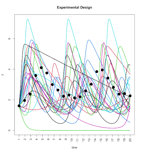
(a)

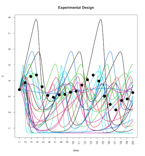
(b)

Figure 5: Computer model training runs and field data for Lotka-Volterra system of ODEs. The black dots are the observed noisy field data, while the colored lines denote the curves generated through differing ODE parameter design points.

To motivate the ecological model, we briefly overview the Lotka-Volterra equations, which describe a mechanism by which predator and prey population sizes oscillate. The equations generating this oscillatory system are

$$\begin{split}\frac{du_{t}}{dt}&=\eta_{1}u_{t}-\eta_{2}u_{t}v_{t}\\ \frac{dv_{t}}{dt}&=-\eta_{3}v_{t}+\eta_{4}u_{t}v_{t}.\end{split}$$ (23)

For our noisy field observations, we utilize the data recorded on the Canadian lynx and snowshoe hare population sizes (Hewitt, 1917). Within (23), $\eta_{1}$ represents the growth rate of the prey population, while $\eta_{2}$ controls the rate of prey population shrinkage relative to the product of the population sizes. Likewise, $\eta_{3}$ represents the rate of population loss within the predator population, and $\eta_{4}$ controls the growth relative to the product of both populations. To formulate weekly informative priors for these parameters, we take $\eta_{1},\eta_{3}\sim\mathcal{N}(1,.5)$ to center the rate of change of both populations around their current sizes. Additionally, we take $\eta_{2},\eta_{4}\sim\mathcal{N}(0.05,0.05)$ to restrain the growth and shrinkage of the respective populations to be a small percentage of the product of the two. We generate training data generated from these priors over a Latin hypercube design as the collection of computer experiments, shown in Figure 5; black dots indicate observed field data.

Table 1 presents the Root Mean Square Errors (RMSE) for the SSGP framework with and without the spatial-temporal bias and for a straightforward nonlinear regression approach that numerically solves the ODE within each iteration of a Hamiltonian Monte Carlo (HMC) algorithm as implemented in the Stan software (https://mc-stan.org/). The SSGP approach requires orders of magnitude fewer numerical solutions while producing very competitive predictive accuracy. In particular, the incorporation of the spatial-temporal bias term in the SSGP improves the RMSE by about 31% from that of the SSGP without the bias term and by about 7.6% from solving the ODE within an HMC fitting algorithm.

Model	RMSE	No. of ODE Solves
SSGP (no bias)	0.301	50
SSGP (with bias)	0.207	50
HMC-ODE	0.224	10000

Table 1: Comparison between directly solving the ODEs in (23) for each MCMC iteration and the SSGP emulation/calibration approach with and without model discrepancy. The SSGP approach requires orders of magnitude fewer numerical solutions for comparable predictive accuracy.

To apply our methodology with notation from Section 2, let $\bm{y}_{t}=(u_{t},v_{t})^{\top}$. As we make use of an AR(1) specification for the state-space component, $\bm{F}_{t}=[u_{t-1},v_{t-1}]$ and $\bm{G}_{t}=\bm{I}$. For all parameters in both models, we find strong prior-to-posterior learning after 10,000 samples posterior samples. After normalizing priors and posteriors to $[0,1]$, Figure 6 shows slightly wider posteriors for the SSGP fit versus the output from Stan. This is intuitive, since our SSGP is trained on only 50 model runs, whereas the Stan code computes the numerical solutions at each iteration of the MCMC. The time used to fit both models was similar, indicating the SSGP could greatly reduce computational effort if model evaluations were instead expensive.

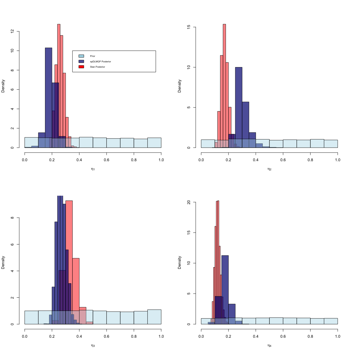
(a)

Figure 6: SSGP versus Stan posteriors for Lotka-Volterra calibration. The ODE model in Stan centers a Gaussian on log-numerical solutions to the system and results in slightly tighter posteriors due to a much larger budget of 10K ODE solves. The emulation/calibration approach achieves comparable performance with a budget of only 50 solves. Strong prior-to-posterior learning is evident in both models.

This initial application illustrates that our methodology provides comparable performance to directly solving the system of differential equations, but in the following examples the computer model may be too expensive to evaluate iteratively within an MCMC scheme.

3.2 Nonlinear Partial Differential Equation Calibration

We apply our methodology to a spatiotemporal model arising from a set of coupled nonlinear PDEs, which are a natural way to describe the dynamics of a continuous outcome across space and time. We model use the set of coupled PDEs shown in (24). This mechanistic system is popular within the applied mathematics community to capture qualitative behavior of spreading infection dynamics (Noble, 1974; Keeling and Rohani, 2008). Literature studying such systems of PDEs often focus on proving various mathematical properties with no discussion about parameter inference or connections to real-world data or field measurements. Specifically, Zhang and Wang (2014) posit the existence of traveling waves in an influenza outbreak for a system such as (24), but omit discussion of parameter inference. See Figure 7 for a visualization of this traveling wave phenomena when two seeding locations are used as initial sources of the disease. To motivate the system of equations under study, we modify a standard SIR compartment model by including a Laplacian term to induce diffusion of the populations over space. In this model, disease transmission is predominantly a localized process where transmission is most likely between nearby locations. Movement of individuals then facilitates the geographical spread of infectious diseases. Such a process may be captured through the following system

$$\begin{split}\frac{\partial S_{t}(\bm{s})}{\partial t}&=-\eta_{1}\frac{S_{t}(\bm{s})I_{t}(\bm{s})}{N}+\alpha_{1}\nabla^{2}S_{t}(\bm{s})\\[4.0pt] \frac{\partial I_{t}(\bm{s})}{\partial t}&=\eta_{1}\frac{S_{t}(\bm{s})I_{t}(\bm{s})}{N}-\eta_{2}I_{t}(\bm{s})+\alpha_{2}\nabla^{2}I_{t}(\bm{s})\\[4.0pt] \frac{\partial R_{t}(\bm{s})}{\partial t}&=\eta_{2}I_{t}(\bm{s})+\alpha_{3}\nabla^{2}R_{t}(\bm{s}),\end{split}$$ (24)

where $\nabla^{2}f_{t}(\bm{s})=\sum_{i=1}^{d}{\partial^{2}f_{t}(\bm{s})}/{\partial\bm{s}_{i}^{2}}$. In applying our methodology, the training data is generated through the numerical solution of (24) for fixed parameter setting $\bm{x}=(\eta_{1}^{\prime},\eta_{2}^{\prime},\alpha_{1}^{\prime},\alpha_{2}^{\prime},\alpha_{3}^{\prime})$. The outcome data $y_{t}(\bm{s},\bm{x})$ is taken to me the infection counts at a location at a location and time, namely $I_{t}(\bm{s})$. For our experiment, we fix in (24) $\alpha_{1}=\alpha_{3}=0$ to induce the most heterogenous spatial dynamics by only allowing infections to diffuse across space. We add synthetic Gaussian error with unit variance to generate the field data $\bm{z}_{1:T}$ for a setting disjoint from the computer model training set.

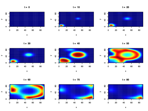
Figure 7: Spatiotemporal dynamics of coupled nonlinear partial differential equations. Lighter color indicates larger function values. Wave-like dynamics radiating outwards from initial seeding locations are apparant.

We utilize the R package ReacTran (Soetaert and Meysman, 2012) developed to solve the system across the design space of parameter values. The spatial domain consists of a $100\times 100$ grid resulting in 10,000 spatial locations; dynamics are shown in Figure 7. To reduce the dimension of the problem, we chose a set of 50 knot locations on a grid across the spatial domain. Figure 8 evinces strong Bayesian learning of calibration parameter values.

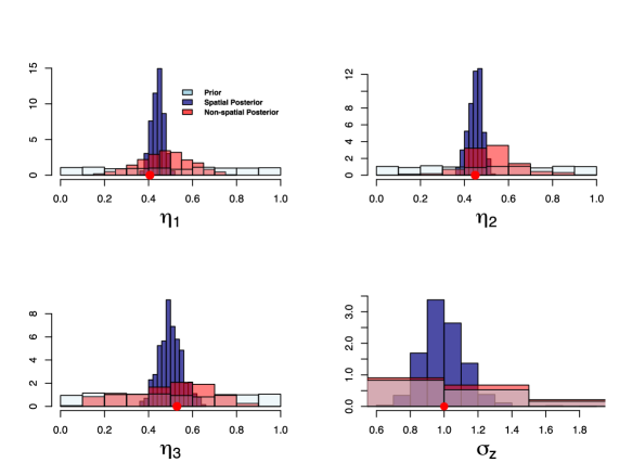
Figure 8: Posteriors for nonlinear PDE calibration. In blue, the fully spatial model in comparison to the seemingly unrelated emulation model that ignores spatial structure. Parameter posteriors are tighter in the fully hierarchical model and result in a much higher GRS value in Table 2.

Table 2 presents model comparisons using the GRS defined in (22), RMSE and the required number of PDE solves. We chose as comparison the fully heterogeneous model of (17) to illustrate the effect of completely ignoring spatial structure. As each ReacTran numerical solution took approximately 10 seconds, it would be costly to repeat this operation iteratively within a naive MCMC sampler. Instead, we find that our SSGP model is effectively capturing the PDE system behavior and enabling efficient inference that circumvents the costly operation of repeatedly solving the system of equations on a large spatial domain.

Model	GRS	RMSE	No. of PDE Solves
heterogeneous model	-1107	2.32	25
spatial model	-179	1.30	25

Table 2: Comparison between heterogeneous spatial model of (17) and fully hierarchical spatial model of (2) for parameter inference in systems on nonlinear PDEs. Both GRS and RMSE strongly favor the fully hierarchical spatial model.

3.3 Calibrating a Computer Simulation with Network Output

Network science studies how the macrostructure of interconnected systems such as telecommunication, economic, cognitive, or social networks affect global dynamics (Watts and Strogatz, 1998). Within a network, nodes represent discrete entities, and edges represent relations. Of prominent interest in applied modeling is understanding how global structure affects spread of a quantity throughout the system, termed network activation or network diffusion. To date, there exist various statistical software packages implementing diffusion or contagion processes across networks (Vega Yon and Valente, 2021; Siew, 2019). These computer simulations may be deterministic or stochastic in nature, though there exists a theoretical relation between the two (Mozgunov et al., 2018). We focus on calibrating a deterministic computer model popular within psychology and psycholinguistics communities (Chan and Vitevitch, 2009; Vitevitch et al., 2011). The spreadr package (Siew, 2019) implements this network diffusion simulation but ignores the calibration problem, justifying use of our methodology.

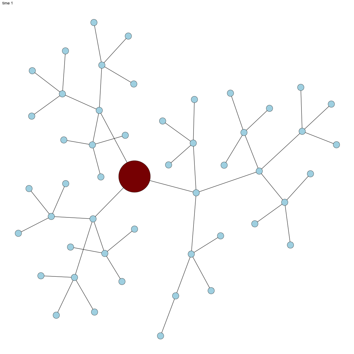
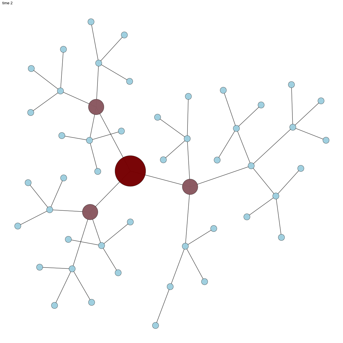
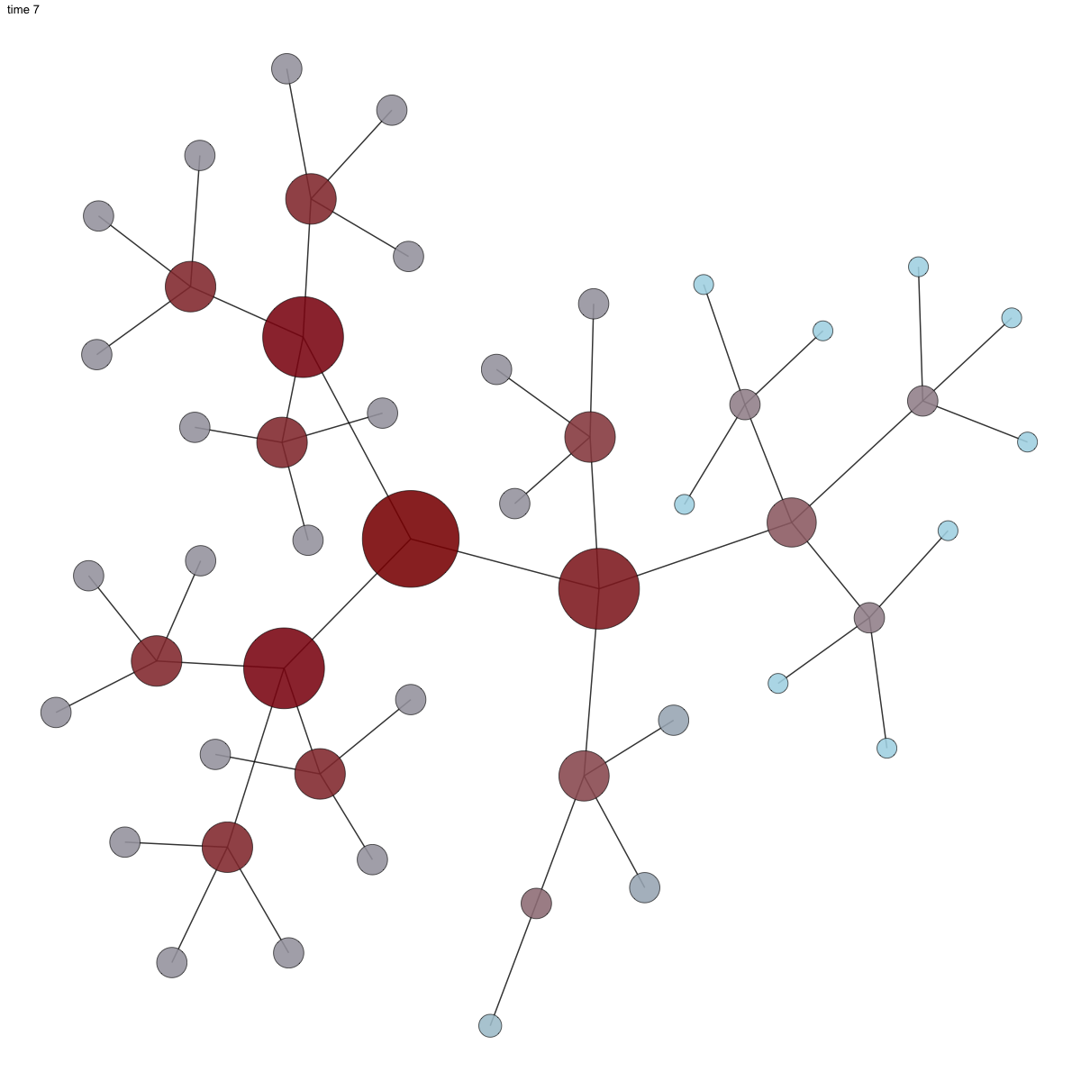
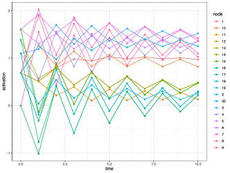
Figure 9: Individual node dynamics across the network. Each line corresponds to an activation level for a specific node over time.

We now define notation necessary for understanding the inputs to this computer simulation. For a network with $n$ nodes, two parameters control the activation spread, known as retention and decay, denoted as $r$ and $d$ respectively.

• $r$ - a scalar or a vector of length $n$ that controls the proportion of activation retained by a node at each time step of the simulation.

• $d$ - a scalar that controls the proportion of activation that is lost at each time step of the simulation.

There are three quantities of interest that define how activation spreads dynamically over time as functions of $r$ and $d$: reservoir, outflow, and inflow. These are defined as follows:

• $\text{reservoir}(t,n)=r\times\text{inflow}(t,n)$.

• $\text{outflow}(t,n)=\dfrac{(1-d)(1-r)\times\text{inflow}(t,n)}{\text{deg}(n)}$.

• $\text{inflow}(t,n)=\sum_{i=1}^{\text{deg}(n)}\text{outflow}(t-1,n_{i})+\text{reservoir}(t-1,n)$, where $\text{deg}(n)$ denotes the number of connections to node $n$.

The computer simulation then computes these quantities for each node in the network, thereby algorithmically generating dynamics. A visualization of the spatiotemporal spreading dynamics is show in Figure 9.

As in the previous section, we use a space-filling design to generate a small collection of plausible values for the parameters, after which we pick a random validation point not included in the training set. Similar to the setting with the PDEs, we see in Table 3 that information is lost when not accounting for spatial structure. Specifically, we see 29.3% and 13.7% improvements in the GRS for the spatial model over the heterogenous model, respectively, using the same computer model runs.

Model	GRS	RMSE	No. of computer model runs
heterogeneous model	1656	0.110	25
spatial model	2142	0.095	25

Table 3: Comparison between heterogeneous spatial model of (17) and fully hierarchical spatial model of (2). Both GRS and RMSE again strongly favor the fully hierarchical spatial model. Though parameter uncertainty is not adequately captured in the seemingly unrelated emulator model, point estimates are similar to the fully hierarchical.

After 10,000 posterior draws, the prior-to-posterior learning is evident in Figure 10 and demonstrates our methodology is capable of calibrating a computer model generating dynamics across a network. Although it is possible to define a Gaussian process over a graph (Venkitaraman et al., 2020), for this application we fix the correlation structure to arise from the adjacency matrix.

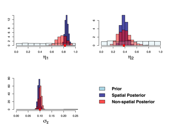
Figure 10: Network diffusion calibration posteriors. The lower uncertainty in the hierarchical model indicates pooling of information across node locations, lost in the heterogeneous model. Posterior mode point estimates are roughly similar.

4 Discussion

We have devised a Bayesian hierarchical framework for the emulation and calibration of dynamically evolving spatiotemporal mechanistic systems. Our approach is broadly applicable across a variety of application areas as demonstrated through a series of examples. Building upon the rich literature on state-space extensions to nonlinear systems (such as nonlinear PDEs explored in Wang et al., 2021, but without melding of field observations) can yield deliver full Bayesian inference using more accurate and flexible emulators. Additionally, the applicability of our model to network-like structures suggests that our methodology could also be applied for calibration of agent-based models evolving over space. Further scalability of our model by making use of spatial partitioning (Gramacy and Lee, 2007). Our dynamic spatiotemporal approach is likely to work well in calibrating computer models with low to medium-dimensional parameter input spaces. For high-dimensional computer simulations, inference of Gaussian process hyperparameters becomes cumbersome due to the Metropolis-Hastings steps required. Therefore, a sequential screening procedure may be employed to identify the most influential parameters (Welch et al., 1992; Merrill et al., 2021). Extensions to generalized dynamic linear models (West et al., 1985) will enable analysis of non-Gaussian data. Lastly, the burgeoning field of sequential Monte Carlo analysis is applicable to build more general statistical emulators within this framework (Hirt and Dellaportas, 2019). We developed our methods in C++ with functions available in R by way of the Rcpp package (Eddelbuettel and François, 2011).

5 Appendix

This appendix provides further details on customizing our model based on knowledge of the underlying dynamical system of which we seek to emulate and calibrate. Additionally, Section 5.2 provides further algorithmic derivation for the backward sampling of the non-Gaussian state-space component in our model. For our example computations, we work with a state-space model of the form

$$\begin{split}\bm{y}_{t}&=\bm{F}_{t}\bm{\theta}_{t}+\bm{\varepsilon}_{t},\quad\bm{\varepsilon}_{t}\stackrel{{\scriptstyle\text{ind.}}}{{\sim}}\mathcal{N}_{N}(0,v_{t}\bm{V})\\ \bm{\theta}_{t}&=\bm{G}\bm{\theta}_{t-1}+\bm{\tau}_{t},\quad\bm{\tau}_{t}\stackrel{{\scriptstyle\text{ind.}}}{{\sim}}\mathcal{N}_{p}(0,v_{t}\bm{W})\\ v_{t}^{-1}&=\dfrac{\gamma_{t}}{\omega}v_{t-1}^{-1},\quad\gamma_{t}\stackrel{{\scriptstyle\text{ind.}}}{{\sim}}\mathcal{B}(\omega n_{t-1},(1-\omega)n_{t-1}),\end{split}$$ (25)

which can easily be connected to the SSGP emulator of (5). Notice the time-invariance of the state transition matrix $\bm{G}$ for illustration purposes.

5.1 Finite Difference Methods for Parameterizing the Emulator

Our parameterization of $\bm{G}$ is inspired through expression (24) and example 2 of Section 3. Consider the heat equation in 1-dimensional space and time

$$\frac{\partial\theta_{t}(s)}{\partial t}=\alpha\frac{\partial^{2}\theta_{t}(s)}{\partial x^{2}}=\alpha\nabla^{2}\theta_{t}(s).$$ (26)

We now discretize time across a grid of $\Delta_{t}$ and form a forward difference approximation of the left-hand side, i.e,.

$$\frac{\partial\theta_{t}(s)}{\partial t}\approx\frac{\theta_{t+\Delta_{t}}(s)-\theta_{t}(s)}{\Delta_{t}}\text{ for small }\Delta_{t}.$$ (27)

Applying the central difference approximation over space twice to the right-hand side of (26) results in the approximate Laplacian

$$\begin{split}\alpha\nabla^{2}\theta_{t}(s)&\approx\frac{\theta_{t}(x+\Delta_{s})-2\theta_{t}(s)+\theta_{t}(x-\Delta_{s})}{\Delta_{s}^{2}}\text{ for small }\Delta_{s}.\end{split}$$ (28)

We now equate (27) and (28) to form the Markov evolution for the latent process and connect to the state-space model of (25), resulting in

$$\begin{split}{\theta_{t+\Delta_{t}}(s)}&=\theta_{t}(s)+\alpha\frac{\Delta_{t}}{\Delta_{s}^{2}}\Big{\{}\theta_{t}(x+\Delta_{s})-2\theta_{t}(s)+\theta_{t}(x-\Delta_{s})\Big{\}}\\ &=(1-2\alpha\frac{\Delta_{t}}{\Delta_{s}})\theta_{t}(s)+\alpha\frac{\Delta_{t}}{\Delta_{s}}\theta_{t}(x+\Delta_{s})+\alpha\frac{\Delta_{t}}{\Delta_{s}}\theta_{t}(x-\Delta_{s})\\ &=g_{1}\theta_{t}(s)+g_{2}\theta_{t}(x+\Delta_{s})+g_{3}\theta_{t}(x-\Delta_{s}).\end{split}$$ (29)

After specifying a Dirichlet boundary condition of zero for boundary points and collecting all spatial locations at time $t$ together, we may write a vectorized version of (29) as $\bm{\theta}_{t+\Delta_{t}}=\bm{G}\bm{\theta}_{t}$, where $\bm{G}$ is a tri-diagonal matrix of the form

$$\bm{G}=\left[\begin{array}[]{cccccc}g_{1}&g_{2}&&&&\\ g_{3}&g_{1}&g_{2}&&&\\ &g_{3}&\ddots&\ddots&&\\ &&\ddots&\ddots&g_{2}&\\ &&&g_{3}&g_{1}&g_{2}\\ &&&&g_{3}&g_{1}\end{array}\right]$$ (30)

We may generalize the previous calculation to different advection-diffusion forms for different applications such as, for example,

$$\begin{split}\frac{\partial\bm{\theta}(s_{1},s_{2})}{\partial t}=\frac{\partial}{\partial s_{1}}\left(a(s_{1},s_{2})\frac{\partial\bm{\theta}(s_{1},s_{2})}{\partial s_{1}}\right)+\frac{\partial}{\partial s_{2}}\left(b(s_{1},s_{2})\frac{\partial\bm{\theta}(s_{1},s_{2})}{\partial s_{2}}\right)\\ +u(s_{1},s_{2})\frac{\partial\bm{\theta}(s_{1},s_{2})}{\partial s_{1}}+v(s_{1},s_{2})\frac{\partial\bm{\theta}(s_{1},s_{2})}{\partial s_{2}},\end{split}$$ (31)

or introduce coefficients that vary over time and space (Gelfand et al., 2003) to induce a time-varying $\bm{G}_{t}$. This flexibility demonstrates the applicability of our emulator framework to broad application areas.

5.2 Non-Gaussian Filtering and Smoothing Algorithm

In this section, we derive the smoothing expressions and algorithm for the non-Gaussian component of our model. Recall the precision is allowed to evolve stochastically through $v_{t}^{-1}={\gamma_{t}}v_{t-1}^{-1}/{\omega}$ where $\gamma_{t}\stackrel{{\scriptstyle\text{}}}{{\sim}}\mathcal{B}(\omega n_{t-1},(1-\omega)n_{t-1})$ and $\omega\in(0,1].$ In this way, $v_{t}^{-1}$ evolves from $v_{t-1}^{-1}$ through a random multiplicative shock with expected value $\mathbb{E}[\gamma_{t}/\omega]=1$. To detail the explicit computation required for sampling, assume first $v_{t-1}^{-1}|\bm{y}_{1:t-1}\stackrel{{\scriptstyle\text{}}}{{\sim}}\mathcal{G}(n_{t-1},d_{t-1})$ and $\gamma_{t}\stackrel{{\scriptstyle\text{}}}{{\sim}}\mathcal{B}(\omega n_{t-1},(1-\omega)n_{t-1})$, the product of these random variates is distributed Gamma. This is quickly shown by representing $\gamma_{t}$ as a ratio of appropriate Gamma random variables and inverting the transformation to subsequently apply standard change of variable calculations. Through induction, this implies the forward filtering operation maintains the Gamma form.

The algorithm for sampling from the smoothing distribution for the precision is now derived. The smoothing distribution in general is written

$$\begin{split}p\left(v_{0:T}^{-1}\mid\bm{y}_{1:T}\right)=\prod_{t=0}^{T}p\left(v^{-1}_{t}\mid v^{-1}_{t+1},\ldots,v^{-1}_{1:T},\bm{y}_{1:T}\right)=p\left(v^{-1}_{t}\mid\bm{y}_{1:T}\right)\prod_{t=1}^{n-1}p\left(v^{-1}_{t}\mid v^{-1}_{t+1},\bm{y}_{t}\right),\end{split}$$ (32)

where it is straightforward to obtain samples from $p(v_{t}^{-1}|v_{t+1}^{-1},\bm{y}_{1:T})$. We first show the multiplicative Markov transition model is proportional to a shifted Gamma distribution by multiplying scaled Beta and Gamma densities:

$$\begin{split}p(v_{t-1}^{-1}&|v_{t}^{-1},\bm{y}_{1:T})\propto p(v_{t}^{-1}|v_{t-1}^{-1},\bm{y}_{1:T})p(v_{t-1}^{-1}|\bm{y}_{1:t-1})\\ &\propto\left(\frac{\omega}{v_{t-1}^{-1}}\right)\left(\dfrac{\omega v_{t}^{-1}}{v_{t-1}^{-1}}\right)^{\omega n_{t-1}-1}\left(1-\dfrac{\omega v_{t}^{-1}}{v_{t-1}^{-1}}\right)^{(1-\omega)n_{t-1}-1}\left(v_{t-1}^{-1}\right)^{n_{t-1}-1}\exp(-d_{t-1}v_{t-1}^{-1})\\ &\propto(v_{t-1}-\omega v_{t}^{-1})^{(1-\omega)n_{t-1}-1}\exp(-d_{t-1}v_{t-1}^{-1})\\ &\propto\text{Shifted-Gamma}(v_{t-1}^{-1};(1-\omega)n_{t},d_{t},\omega v_{t}^{-1}),\end{split}$$ (33)

where $(1-\omega)n_{t-1}$ is the shape, $d_{t}$ is the rate, and $\omega v_{t}^{-1}$ is the shift. This gives a recurrence relation to algorithmicaly sample from the smoothing distribution, once $v_{t}^{-1}$ is obtained due to the shifting property of a Gamma distribution. This representation then justifies the process of Algorithm 5 line 8.

Algorithm 4 Kalman filter

1:Input: Data $\bm{y}_{1:T}$, Kalman filter starting values $n_{0}$, $d_{0}$, $\bm{m}_{0}$, $\bm{M}_{0}$, and discount factor $\omega$

2:Input: Observation and state transition matrices $\bm{F}_{1:T}$ and $\bm{G}_{1:T}$

3:Input: Correlation matrices $\bm{V}$, $\bm{W}$

4:Output: Filtering distribution parameters at time $t=0,\ldots,T$

5:function Filter($\bm{y}_{1:T},n_{0},d_{0},\bm{m}_{0},\bm{M}_{0},\bm{G}_{1:T},\bm{F}_{1:T},\bm{V},\bm{W}$)

6:     for $t=1$ to $T$ do

7:         # Compute prior distribution $p(\bm{\theta}_{t},v_{t}^{-1}|\bm{y}_{1:t-1})\sim\mathcal{NG}(\bm{a}_{t},\bm{A}_{t},n_{t}^{*},d_{t}^{*}):$

8:         $\bm{a}_{t}\leftarrow\bm{G}_{t}\bm{m}_{t-1},\ \bm{A}_{t}\leftarrow\bm{G}_{t}\bm{M}_{t-1}\bm{G}_{t}^{\top}+\bm{W}$

9:         $n_{t}^{*}\leftarrow\omega n_{t-1},d_{t}^{*}\leftarrow\omega d_{t-1}$

10:         # Compute one-step-ahead forecast $p(\bm{y}_{t}|\bm{y}_{1:t-1})\sim\mathcal{T}(\bm{q}_{t},\bm{Q}_{t}\frac{d_{t^{*}}}{n_{t}^{*}},2n_{t}^{*}):$

11:         $\bm{q}_{t}\leftarrow\bm{F}_{t}\bm{a}_{t},\ \bm{Q}_{t}\leftarrow\bm{F}_{t}\bm{A}_{t}\bm{F}_{t}^{\top}+\bm{V}$

12:         # Compute filtering distribution $p(\bm{\theta}_{t},v_{t}^{-1}|\bm{y}_{1:t})\sim\mathcal{NG}(\bm{m}_{t},\bm{M}_{t},n_{t},d_{t}):$

13:         $\bm{m}_{t}\leftarrow\bm{a}_{t}+\bm{A}_{t}\bm{F}_{t}\bm{Q}_{t}^{-1}(\bm{y}_{t}-\bm{q}_{t}),\ \bm{M}_{t}\leftarrow\bm{A}_{t}-\bm{A}_{t}\bm{F}_{t}^{\top}\bm{Q}_{t}^{-1}\bm{F}_{t}\bm{A}_{t}^{\top}$

14:         $n_{t}\leftarrow n_{t}^{*}+\frac{N}{2},\ d_{t}\leftarrow d_{t}^{*}+\frac{1}{2}(\bm{y}_{t}-\bm{q}_{t})^{\top}\bm{Q}_{t}^{-1}(\bm{y}_{t}-\bm{q}_{t})$

15:     end for

16:     return $\left\{n_{t},d_{t},\bm{a}_{t},\bm{A}_{t},\bm{m}_{t},\bm{M}_{t}\right\}_{t=0}^{T}$

17:end function

Algorithm 5 Backward sampler

1:Input: Filtering parameters and inputs from Algorithm 4

2:Output: Posterior sample from $p(\bm{\theta}_{0:T},v_{0:T}|\bm{y}_{1:T})$

3:function BackwardSample($\left\{n_{t},d_{t},\bm{a}_{t},\bm{A}_{t},\bm{m}_{t},\bm{M}_{t},\bm{G}_{t}\right\}_{t=0}^{T}$)

4:     Draw $v_{T}^{-1}\sim\mathcal{G}(n_{T},d_{T})$

5:     Draw $\bm{\theta}_{T}\sim\mathcal{N}(\bm{m}_{T},v_{T}\bm{M}_{T})$

6:     for $t=T-1$ to $0$ do

7:         Draw $v_{t}^{*}\sim\mathcal{G}((1-\omega)n_{t},d_{t})$

8:         $v_{t}^{-1}\leftarrow\omega v_{t+1}^{-1}+v_{t}^{*}$

9:         $\bm{s}_{t}\leftarrow\bm{m}_{t}+\bm{M}_{t}\bm{G}_{t+1}^{\top}\bm{A}_{t+1}^{-1}\left(\bm{s}_{t+1}-\bm{a}_{t+1}\right)$

10:         $\bm{S}_{t}\leftarrow\bm{M}_{t}-\bm{M}_{t}\bm{G}_{t+1}^{\top}\bm{A}_{t+1}^{-1}\left(\bm{A}_{t+1}-\bm{S}_{t+1}\right)\bm{A}_{t+1}^{-1}\bm{G}_{t+1}\bm{M}_{t}$

11:         Draw $\bm{\theta}_{t}\sim\mathcal{N}(\bm{s}_{t},v_{t}\bm{S}_{t})$

12:     end for

13:     return $\{v_{t},\bm{\theta}_{t}\}_{t=0}^{T}$

14:end function

References

- Banerjee (2017) S. Banerjee. High-Dimensional Bayesian Geostatistics. Bayesian Analysis, 2017.
- Banerjee et al. (2008) S. Banerjee, A. Gelfand, A. Finley, and H. Sang. Gaussian Predictive Process Models for Large Spatial Data Sets. Journal of the Royal Statistical Society. Series B, Statistical methodology, 2008.
- Banerjee et al. (2014) S. Banerjee, B. Carlin, and A. Gelfand. Hierarchical Modeling and Analysis for Spatial Data. CRC Press, 2014.
- Bayarri et al. (2009) M. J. Bayarri, J. O. Berger, and F. Liu. Modularization in Bayesian Analysis, with Emphasis on Analysis of Computer Models. Bayesian Analysis, 2009.
- Carpenter et al. (2017) B. Carpenter, A. Gelman, M. Hoffman, D. Lee, B. Goodrich, M. Betancourt, M. Brubaker, J. Guo, P. Li, and A. Riddell. Stan : A Probabilistic Programming Language. Journal of Statistical Software, 2017.
- Carter and Kohn (1994) C. Carter and R. Kohn. On Gibbs Sampling for State Space Models. Biometrika, 1994.
- Chan and Vitevitch (2009) K. Y. Chan and M. S. Vitevitch. The Influence of the Phonological Neighborhood Clustering-Coefficient on Spoken Word Recognition. Journal of Experimental Psychology: Human Perception and Performance, 2009.
- Cockayne et al. (2017) J. Cockayne, C. Oates, T. Sullivan, and M. Girolami. Probabilistic numerical methods for PDE-constrained Bayesian inverse problems. AIP Conference Proceedings, 2017.
- Datta et al. (2016) A. Datta, S. Banerjee, A. Finley, and A. Gelfand. On nearest-neighbor Gaussian process models for massive spatial data: Nearest-neighbor Gaussian process models. Wiley Interdisciplinary Reviews: Computational Statistics, 2016.
- Datta et al. (2016b) A. Datta, S. Banerjee, A. O. Finley, N. A. S. Hamm, and M. Schaap. Non-separable Dynamic Nearest-Neighbor Gaussian Process Models for Large spatio-temporal Data With an Application to Particulate Matter Analysis. Annals of Applied Statistics, 2016b.
- Eddelbuettel and François (2011) D. Eddelbuettel and R. François. Rcpp: Seamless R and C++ integration. Journal of Statistical Software, 2011.
- Eleftheriadis et al. (2017) S. Eleftheriadis, T. F. Nicholson, M. P. Deisenroth, and J. Hensman. Identification of Gaussian Process State Space Models. In Proceedings of the 31st International Conference on Neural Information Processing Systems, 2017.
- Farah et al. (2014) M. Farah, P. Birrell, S. Conti, and D. D. Angelis. Bayesian Emulation and Calibration of a Dynamic Epidemic Model for A/H1N1 Influenza. Journal of the American Statistical Association, 2014.
- Finley et al. (2009) A. Finley, H. Sang, S. Banerjee, and A. Gelfand. Improving the performance of predictive process modeling for large datasets. Computational statistics & data analysis, 2009.
- Finley et al. (2012) A. Finley, S. Banerjee, and A. Gelfand. Bayesian Dynamic Modeling for Large Space–Time Datasets Using Gaussian Predictive Processes. Journal of Geographical Systems, 2012.
- Finley et al. (2019) A. O. Finley, A. Datta, B. C. Cook, D. C. Morton, H. E. Andersen, and S. Banerjee. Efficient algorithms for bayesian nearest neighbor gaussian processes. Journal of Computational and Graphical Statistics, 28(2):401–414, 2019.
- Frankenburg and Banerjee (2022) I. Frankenburg and S. Banerjee. A Compartment Model of Human Mobility and Early Covid-19 Dynamics in NYC. The New England Journal of Statistics in Data Science, 2022.
- Frühwirth-Schnatter (2006) S. Frühwirth-Schnatter. Finite Mixture and Markov Switching Models. Springer New York, 2006.
- Gamerman et al. (2013) D. Gamerman, T. Rezende, and G. Franco. A Non-Gaussian Family Of State-Space Models With Exact Marginal Likelihood. Journal of Time Series Analysis, 2013.
- Gelfand et al. (2003) A. Gelfand, H.-J. Kim, S. C.F, and S. Banerjee. Spatial Modeling With Spatially Varying Coefficient Processes. Journal of the American Statistical Association, 2003.
- Gelman (2004) A. Gelman. Parameterization and Bayesian Modeling. Journal of the American Statistical Association, 2004.
- Gneiting and Raftery (2007) T. Gneiting and A. Raftery. Strictly Proper Scoring Rules, Prediction, and Estimation. Journal of the American Statistical Association, 2007.
- Gramacy and Lee (2007) R. Gramacy and H. Lee. Bayesian Treed Gaussian Process Models With an Application to Computer Modeling. Journal of the American Statistical Association, 2007.
- Heaton et al. (2019) M. Heaton, A. Datta, A. Finley, R. Furrer, J. Guinness, R. Guhaniyogi, F. Gerber, R. Gramacy, D. Hammerling, M. Katzfuss, F. Lindgren, D. Nychka, F. Sun, and A. Zammit-Mangion. Methods for Analyzing Large Spatial Data: A Review and Comparison. Journal of Agricultural, Biological and Environmental Statistics, 2019.
- Hefley et al. (2017) T. Hefley, M. Hooten, R. Russell, D. Walsh, and J. Powell. When mechanism matters: Bayesian forecasting using models of ecological diffusion. Ecology Letters, 2017.
- Hewitt (1917) G. Hewitt. Conservation of Wild Life in Canada. Nature, 1917.
- Higdon et al. (2004) D. Higdon, M. Kennedy, J. Cavendish, J. Cafeo, and R. Ryne. Combining Field Data and Computer Simulations for Calibration and Prediction. SIAM J. Scientific Computing, 2004.
- Higdon et al. (2008) D. Higdon, J. Gattiker, B. Williams, and M. Rightley. Computer Model Calibration Using High-Dimensional Output. Journal of the American Statistical Association, 2008.
- Hirt and Dellaportas (2019) M. Hirt and P. Dellaportas. Scalable Bayesian Learning for State Space Models using Variational Inference with SMC Samplers. In K. Chaudhuri and M. Sugiyama, editors, Proceedings of the Twenty-Second International Conference on Artificial Intelligence and Statistics, Proceedings of Machine Learning Research. PMLR, 2019.
- Hooten et al. (2013) M. Hooten, M. Garlick, and J. Powell. Computationally Efficient Statistical Differential Equation Modeling Using Homogenization. Journal of Agricultural, Biological, and Environmental Statistics, 2013.
- Kalman (1960) R. Kalman. A New approach to Linear Filtering and Prediction Problems. Journal of basic Engineering, 1960.
- Katzfuss and Guinness (2021) M. Katzfuss and J. Guinness. A General Framework for Vecchia Approximations of Gaussian Processes”. Statistical Science, 2021.
- Keeling and Rohani (2008) M. J. Keeling and P. Rohani. Modeling Infectious Diseases in Humans and Animals. Princeton University Press, 2008.
- Kennedy and O’Hagan (2001) M. Kennedy and A. O’Hagan. Bayesian Calibration of Computer Models. Journal of the Royal Statistical Society Series B, 2001.
- Liu and West (2009) F. Liu and M. West. A Dynamic Modelling Strategy for Bayesian Computer Model Emulation. Bayesian Analysis, 2009.
- Liu and Wu (1999) J. Liu and Y. Wu. Parameter Expansion for Data Augmentation. Journal of the American Statistical Association, 1999.
- Merrill et al. (2021) E. Merrill, A. Fern, X. Fern, and N. Dolatnia. An empirical study of bayesian optimization: Acquisition versus partition. Journal of Machine Learning Research, 2021.
- Mozgunov et al. (2018) P. Mozgunov, M. Beccuti, A. Horvath, T. Jaki, R. Sirovich, and E. Bibbona. A review of the deterministic and diffusion approximations for stochastic chemical reaction networks. Reaction Kinetics, Mechanisms and Catalysis, 2018.
- Murray (2003) J. D. Murray. Mathematical Biology II: Spatial Models and Biomedical Applications. Interdisciplinary Applied Mathematics. 2003.
- Noble (1974) J. Noble. Geographic and Temporal Development of Plagues. Nature, 1974.
- Peruzzi et al. (2022) M. Peruzzi, S. Banerjee, and A. Finley. Highly Scalable Bayesian Geostatistical Modeling via Meshed Gaussian Processes on Partitioned Domains. Journal of the American Statistical Association, 117(538):969–982, 2022.
- Petris et al. (2009) G. Petris, S. Petrone, and P. Campagnoli. Dynamic Linear Models with R. Springer New York, 2009.
- Poole and Raftery (2000) D. Poole and A. E. Raftery. Inference for Deterministic Simulation Models: The Bayesian Melding Approach. Journal of the American Statistical Association, 2000.
- Quiñonero-Candela and Rasmussen (2005) J. Quiñonero-Candela and C. E. Rasmussen. A Unifying View of Sparse Approximate Gaussian Process Regression. Journal of Machine Learning Research, 2005.
- Raissi (2018) M. Raissi. Deep Hidden Physics Models: Deep Learning of Nonlinear Partial Differential Equations. Journal of Machine Learning Research, 2018.
- Salter and Williamson (2019) J. M. Salter and D. B. Williamson. Efficient calibration for high-dimensional computer model output using basis methods, 2019.
- Santner et al. (2003) T. Santner, B. Williams, and W. Notz. The Design and Analysis Computer Experiments. Springer New York, 2003.
- Scott (2002) S. L. Scott. Bayesian Methods for Hidden Markov Models. Journal of the American Statistical Association, 2002.
- Siew (2019) C. Siew. spreadr: An R package to simulate spreading activation in a network. Behavior Research Methods, 2019.
- Soetaert and Meysman (2012) K. Soetaert and F. Meysman. Reactive transport in aquatic ecosystems: Rapid model prototyping in the open source software R. Environmental Modelling & Software, 2012.
- Stan Development Team (2021) Stan Development Team. RStan: the R interface to Stan. 2021. URL https://mc-stan.org/. R package version 2.21.3.
- Struthers and Potter (2019) A. Struthers and M. Potter. Differential Equations: For Scientists and Engineers. Springer Cham, 2019.
- Särkkä (2013) S. Särkkä. Bayesian Filtering and Smoothing. Cambridge University Press, 2013.
- Turner et al. (2010) R. Turner, M. Deisenroth, and C. Rasmussen. State-Space Inference and Learning with Gaussian Processes. In Y. W. Teh and M. Titterington, editors, Proceedings of the Thirteenth International Conference on Artificial Intelligence and Statistics, Proceedings of Machine Learning Research, 2010.
- Vecchia (1988) A. V. Vecchia. Estimation and Model Identification for Continuous Spatial Processes. Journal of the Royal Statistical society, Series B, 1988.
- Vega Yon and Valente (2021) G. Vega Yon and T. Valente. netdiffuseR: Analysis of Diffusion and ContagionProcesses on Networks, 2021.
- Venkitaraman et al. (2020) A. Venkitaraman, S. Chatterjee, and P. Handel. Gaussian Processes Over Graphs. In ICASSP 2020 - 2020 IEEE International Conference on Acoustics, Speech and Signal Processing (ICASSP), 2020.
- Vitevitch et al. (2011) M. Vitevitch, G. Ercal, and B. Adagarla. Simulating Retrieval from a Highly Clustered Network: Implications for Spoken Word Recognition. Frontiers in psychology, 2011.
- Wang et al. (2021) J. Wang, J. Cockayne, O. Chkrebtii, T. Sullivan, and C. Oates. Bayesian numerical methods for nonlinear partial differential equations. Statistics and Computing, 2021.
- Watts and Strogatz (1998) D. J. Watts and S. H. Strogatz. Collective dynamics of ‘small-world’ networks. Nature, 1998.
- Welch et al. (1992) W. J. Welch, R. J. Buck, J. Sacks, H. P. Wynn, T. J. Mitchell, and M. D. Morris. Screening, predicting, and computer experiments. Technometrics, 1992.
- West and Harrison (1997) M. West and J. Harrison. Bayesian Forecasting and Dynamic Models (2nd Ed.). Springer-Verlag, 1997.
- West et al. (1985) M. West, P. J. Harrison, and H. S. Migon. Dynamic Generalized Linear Models and Bayesian Forecasting. Journal of the American Statistical Association, 1985.
- Wikle and Hooten (2010) C. Wikle and M. Hooten. A general science-based framework for dynamical spatio-temporal models. TEST, 2010.
- Wikle et al. (2019) C. Wikle, A. Zammit-Mangion, and N. Cressie. Spatio-Temporal Statistics with R. Chapman & Hall/CRC, 2019.
- Wooldridge (2002) J. M. Wooldridge. Econometric Analysis of Cross Section and Panel Data. MIT Press, 2002.
- Zellner and Ando (2010) A. Zellner and T. Ando. Bayesian and non-Bayesian analysis of the seemingly unrelated regression model with Student-errors, and its application for forecasting. International Journal of Forecasting, 2010.
- Zhang and Wang (2014) T. Zhang and W. Wang. Existence of Traveling Wave Solutions for Influenza Model with Treatment. Journal of Mathematical Analysis and Applications, 2014.