New Features of P$3\delta$ Software.
Insights and Demos

Abstract

This paper presents the software entitled “Partial Pole Placement via Delay Action,” or “P$3\delta$” for short. P$3\delta$ is a Python software with a friendly user interface for the design of parametric stabilizing feedback laws with time-delays for dynamical systems. After recalling the theoretical foundation of the so-called “Partial Pole Placement” methodology we propose as well the main features of the current version of P$3\delta$. We illustrate its use in feedback stabilization of several control systems operating under time delays.

1 Introduction

Time delays often occur in controlling dynamical systems, mainly due to the time required for acquiring, propagating, or processing information. It is commonly accepted that a delay in a control loop induces instability, oscillations and bad performance of the overall scheme. For instance, since the 30s, Callender et al. (1936), Hartree et al. (1937) showed the difficulty of handling delays in control loops for second- and third-order linear time-invariant (LTI) dynamical systems and one of the natural ideas was to compensate it by pre-correction (see, e.g., Porter (1952)).

However, as noted and briefly discussed in Sipahi et al. (2011), in some cases, the delay can have a stabilizing effect. Furthermore, it has been emphasized in Suh and Bien (1979) and Atay (1999) that one may replace the classical proportional-derivative controller by a proportional-delayed controller, using the so-called “average derivative action” due to the delay. Finally, regarding the beneficial effect of the delay, closed-loop stability may be guaranteed for some dynamical systems subject to input delays precisely by the existence of such delays, as pointed out in Niculescu et al. (2010) and the references therein in controlling oscillators by delayed output feedback.

The above reasons explain, in part, an abundant literature on such topics, such as Gu et al. (2003); Michiels and Niculescu (2014); Stépán (1989) and the references therein. It should be mentioned that time-delay dynamical systems are infinite-dimensional systems and there exist several ways to represent their dynamics. In the sequel, their dynamics are represented by delay-differential equations (DDEs). For an introduction on DDEs, we refer to Hale and Verduyn Lunel (1993).

The software P3$\delta$ was introduced in Boussaada et al. (2020a, 2021). The main intention of the authors is to help users interested in stability analysis and stabilization of dynamical LTI systems in the presence of a single delay in closed loop. P3$\delta$ makes use of the so-called multiplicity-induced-dominancy (MID) and partial pole placement methods. More precisely, MID is an unexpected spectral property stating that, in some cases, the characteristic root with maximal multiplicity defines the spectral abscissa of the corresponding characteristic function, i.e., the rightmost root of the spectrum. In control, MID opened a new and interesting perspective relying on the idea of a partial pole placement by reinforcing the use of the delay as a control parameter. For a deeper discussion on these methods, we refer to Amrane et al. (2018); Bedouhene et al. (2020); Boussaada and Niculescu (2018); Boussaada et al. (2020b, 2018b); Mazanti et al. (2021, 2020a, 2020b); Boussaada and Niculescu (2016a); Boussaada and Niculescu (2016b); Boussaada et al. (2016, 2018a); Ma et al. (2022).

The software P3$\delta$ covers DDEs of retarded or neutral type with a single time delay, under the form

$$\textstyle y^{(n)}(t)+a_{n-1}y^{(n-1)}(t)+\dotsb+a_{0}y(t)\\ \textstyle+b_{m}y^{(m)}(t-\tau)+\dotsb+b_{0}y(t-\tau)=0,$$ (1)

under appropriate initial conditions, where $\tau>0$ is the positive delay, $y$ is the real-valued unknown function, $n$ and $m$ are nonnegative integers with $n\geq m$, and $a_{0},\dotsc,a_{n-1},b_{0},\dotsc,b_{m}$ are real coefficients.

To address the stability analysis of LTI DDEs, the software P3$\delta$ relies on spectral methods (see, e.g., Hale and Verduyn Lunel (1993); Michiels and Niculescu (2014)), which consist on the study of the complex roots of a characteristic function of the system. The characteristic function $\Delta:\mathbb{C}\to\mathbb{C}$ of (1) is given by

$$\Delta(s)=s^{n}+\sum_{k=0}^{n-1}a_{k}s^{k}+e^{-s\tau}\sum_{k=0}^{m}b_{k}s^{k},$$ (2)

and (1) is exponentially stable if and only if the spectral abscissa $\gamma=\sup\{\operatorname{Re}s\mid\Delta(s)=0\}$ satisfies $\gamma<0$.

P3$\delta$ considers that $b_{0},\dotsc,b_{m}$ are free parameters. In its “Generic” mode, $a_{0},\dotsc,a_{n-1}$ are also assumed to be free and $\tau$ is fixed while, in its “Control-oriented” mode, $a_{0},\dotsc,a_{n-1}$ are assumed fixed and $\tau$ can be assumed either free or fixed. The “Control-oriented” mode is usually suitable for control applications, as illustrated in Section 3.

The strategy used by P3$\delta$ to stabilize a time-delay system is to tune its free parameters to assign finitely many roots while also guaranteeing that the rightmost root on the complex plane is among the chosen ones. Two main properties define such a strategy: (i) first, assigning a real root of maximal multiplicity and proving that this root is necessarily the rightmost root of the characteristic quasipolynomial, a property which has been named multiplicity-induced-dominancy, or MID for short, and (ii) second, assigning a certain amount of real roots, typically equally spaced for simplicity, and proving that the rightmost root among them is also the rightmost root of the characteristic quasipolynomial, a property which has been named coexisting real roots-induced-dominancy, or CRRID for short, in Amrane et al. (2018); Bedouhene et al. (2020).

The MID property for (1) was shown, for instance, in Boussaada et al. (2018b) in the case $(n,m)=(2,0)$, in Boussaada et al. (2020b) in the case $(n,m)=(2,1)$ (see also Boussaada and Niculescu (2018)), in Mazanti et al. (2021) in the case of any positive integer $n$ and $m=n-1$ (see also Mazanti et al. (2020a)), and more recently in Boussaada et al. (2022) for arbitrary $n\geq m$. It was also studied for neutral systems of orders $1$ and $2$ in Ma et al. (2022); Benarab et al. (2020) and extended to complex conjugate roots of maximal multiplicity in Mazanti et al. (2020b). The CRRID property was shown, for instance, in Amrane et al. (2018) in the cases $(n,m)=(2,0)$ and $(n,m)=(1,0)$, and in Bedouhene et al. (2020) in the case of any positive integer $n$ and $m=0$.

In all the above cases, the maximal multiplicity of a real root or, equivalently, the maximal number of coexisting simple real roots is $n+m+1$. The idea to exploit the nature of (real or complex) open-loop roots in control design was proposed for second-order systems in Boussaada et al. (2020b) and extended for arbitrary order systems with real-rooted plants in Balogh et al. (2020, 2022).

As mentioned earlier, P3$\delta$ allows for the parametric design of stabilizing feedback laws with time-delays by exploiting the MID and CRRID properties briefly presented above. The present paper describes the new functionalities of P$3\delta$ and provides some illustrative examples for its use.

2 New features of P3$\delta$

2.1 New features of the online version

After a first iteration of the software, P3$\delta$ Online was completed with new features (Figure 1) that enrich the software and improve user experience. The one-click online version of P3$\delta$ is still hosted on Binder, which provides a personalized computing environment directly from a GitHub repository. The P3$\delta$ team continued to develop the online software in Python, using the dynamic Jupyter Notebook format and with an user interface built using interactive widgets from Python’s ipywidgets module. P3$\delta$ is freely available for download on https://cutt.ly/p3delta, where installation instructions, video demonstrations, and the user guide are also available.

P3$\delta$ Online is based on the program of the executable version and enriched with exclusive features to this version. The online software includes features from the “Generic MID”, “Control-oriented MID”, and “Generic CRRID” modes of P3$\delta$ described in Boussaada et al. (2021, 2020a).

In the “Generic MID” mode, the online version of the software returns the spectrum distribution as well as a normalized quasipolynomial which admits a root of multiplicity $n+m+1$ at the origin. In the “Control-oriented MID” mode, the online version of software returns the admissibility region, a normalized quasipolynomial which admits a root of multiplicity $m+2$ at the origin, and an illustration of the bifurcation of the root of multiplicity $m+2$ with respect to variations of the delay $\tau$.

The first new feature of P3$\delta$ Online is the addition of a “Home” tab that contains information about the project and the software settings. Two settings are currently available: the appearance of notifications and the activation of the software limits.

In the “Generic MID” mode, the spectral distribution analysis now provides two new forms of the output equation, Factorized integral equation and Hypergeometric factorization. In the “Control-oriented MID” mode, it is now possible to choose the value of the discretization step as well as the number of iterations for the $\tau$ sensitivity plot.

Finally, the P3$\delta$ team has developed a new feature to export the results obtained in the software in the format of a report automatically written in a PDF file. The user has the choice of which calculation mode results they want to export and can save the report directly on their computer.

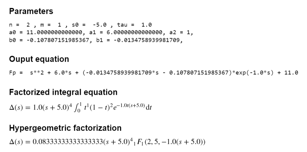
(a)

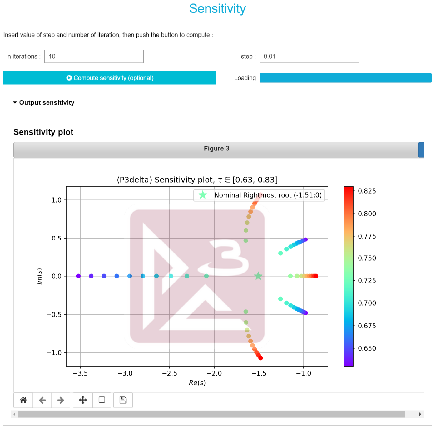
(b)

(c)

Figure 1: Illustration of the different new features of P3$\delta$ Online.

2.2 Assignment admissibility region

Given a system, the definition of valid hyper-parameters ($s_{0}$ and $\tau$) can sometimes be difficult. In order to help users getting a better idea of the admissibility ranges of $s_{0}$ and $\tau$, P3$\delta$ has an admissibility region plotting feature which will be described in this section. Note that this feature is only available when using “Control-oriented MID” as it currently is the only mode with constraints on $(s_{0},\tau)$.

More precisely, given $a_{0},\dotsc,a_{n-1}$, the admissibility region is defined as the set of pairs $(s_{0},\tau)\in\mathbb{R}\times(0,+\infty)$ for which there exist real coefficients $b_{0},\dotsc,b_{m}$ such that $s_{0}$ is a root of $\Delta$ of multiplicity at least $m+2$ when the delay is $\tau$. To compute such a region, we first express the coefficients $(b_{i})_{0\leq i\leq m}$ in terms of $(a_{i})_{0\leq i\leq n-1}$, $s_{0}$, and $\tau$ by using the $m+1$ equations $\Delta^{(k)}(s_{0})=0$, $k\in\{0,\dotsc,m\}$. As those equations are linear in the $m+1$ variables $b_{0},\dotsc,b_{m}$, this linear system admits a unique solution. We then replace these expressions of $(b_{i})_{0\leq i\leq m}$ in the equation $\Delta^{(m+1)}(s_{0})=0$, obtaining an algebraic relation between $s_{0}$, $\tau$, and the coefficients $(a_{i})_{0\leq i\leq n-1}$. By construction, this is a necessary and sufficient condition for $s_{0}$ to be a root of multiplicity at least $m+2$ of $\Delta$ and, since the coefficients $(a_{i})_{0\leq i\leq n-1}$ are known in this mode, this algebraic equation characterizes the admissibility region.

In P3$\delta$, the computations leading to this admissibility region is done by following the previously mentioned steps in a symbolic way using the sympy package. Only the part of the admissibility region in the rectangle $[s_{0,\min},0]\times[0,\tau_{\max}]$ is displayed, where $s_{0,\min}<0$ and $\tau_{\max}>0$ are values selected by the user.

3 Applications of P3$\delta$

To illustrate P3$\delta$, we present some applications of the software.

3.1 Harmonic oscillator

Consider a controlled harmonic oscillator described by

$$y^{\prime\prime}(t)+y(t)=u(t),$$ (3)

where $y(t)\in\mathbb{R}$ is the instantaneous state of the oscillator available to measurement, the control input $u(t)$ corresponds to the applied force, and the coefficients of the equation were normalized. We assume that the control input is given by a delayed proportional-derivative controller

$$u(t)=-\beta y(t-\tau)-\alpha y^{\prime}(t-\tau),$$ (4)

where $\alpha$ and $\beta$ are the coefficients of the controller and $\tau>0$ is the delay. The characteristic equation of the closed-loop system is thus

$$\Delta(s)=s^{2}+1+(\beta+\alpha s)e^{-s\tau}.$$ (5)

The polynomial corresponding to the non-delayed term in (5) is of degree $n=2$, while that corresponding to the delayed term is of degree $m=1$. The degree of the quasipolynomial $\Delta$ is thus $n+m+1=4$.

Let us use P3$\delta$ in order to place a root of multiplicity $m+2=3$ at some $s_{0}\in\mathbb{R}$. One should first input into P3$\delta$ the values of the known coefficients of the quasipolynomial $\Delta$ from (5), i.e., the coefficients of the polynomial corresponding to the non-delayed term. After introducing the data corresponding to (5) into P3$\delta$, one obtains the plot of the admissibility region, as in Figure 2.

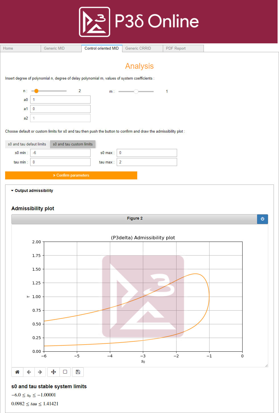
Figure 2: Data input and admissibility plot for the harmonic oscillator.

Based on Figure 2, one observes that the method used by P3$\delta$ allows for the stabilization of the system if the delay is at most approximately $1.4$. After inputting the value of the delay, P3$\delta$ will compute the root $s_{0}$ and the coefficients $\alpha$ and $\beta$, and trace the spectrum distribution of (5) with the derived values. In the present example, the corresponding screen of P3$\delta$ is shown in Figure 3, where, for $\tau=1$, one obtains $s_{0}=-1$, $\alpha=0$, and $\beta\approx-0.7358$.

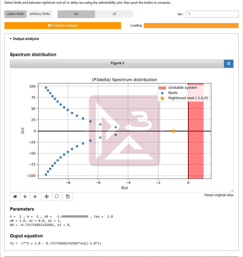
Figure 3: Computed values and spectrum distribution for the harmonic oscillator.

3.2 Inverted pendulum

As a second example of application of P3$\delta$, we consider the stabilization of an inverted pendulum from Figure 4, in which a stick of mass $m$ and length $\ell$ is placed over a cart and can rotate freely around the attachment point $A$. The cart can move along a rail and an external force $F$ is applied on the cart, and we assume that the mass of the cart is negligible compared to the mass of the stick. We denote by $\varphi$ the angle between the stick and the upward vertical direction. In this case, following Molnar et al. (2021), the linearization of the dynamics of $\varphi$ around the unstable equilibrium $\varphi=0$ is

$$\textstyle\varphi^{\prime\prime}(t)-\frac{mg\ell}{2I}\varphi(t)=\frac{\ell}{2I}F(t),$$ (6)

where $I=\frac{1}{12}m\ell^{2}$ is the moment of inertia of the stick and $g$ is the gravitational acceleration. For the numerical application, we will consider $m=10$ kg and $\ell=10$ m, in which case $I\approx 83.33$ kg m².

Figure 4: Inverted pendulum on a cart.

We wish to stabilize the origin of (6) by a delayed PD feedback of the angular position, i.e., we wish to apply

$$F(t)=-K_{p}\varphi(t-\tau)-K_{d}\varphi^{\prime}(t-\tau),$$

yielding a closed-loop system with characteristic equation

$$\textstyle\Delta(s)=s^{2}-\frac{mg\ell}{2I}+\left(\frac{K_{p}\ell}{2I}+\frac{K_{d}\ell}{2I}s\right)e^{-s\tau}.$$ (7)

Note that, here, the delay $\tau$ can be seen as a design parameter, together with $K_{p}$ and $K_{d}$.

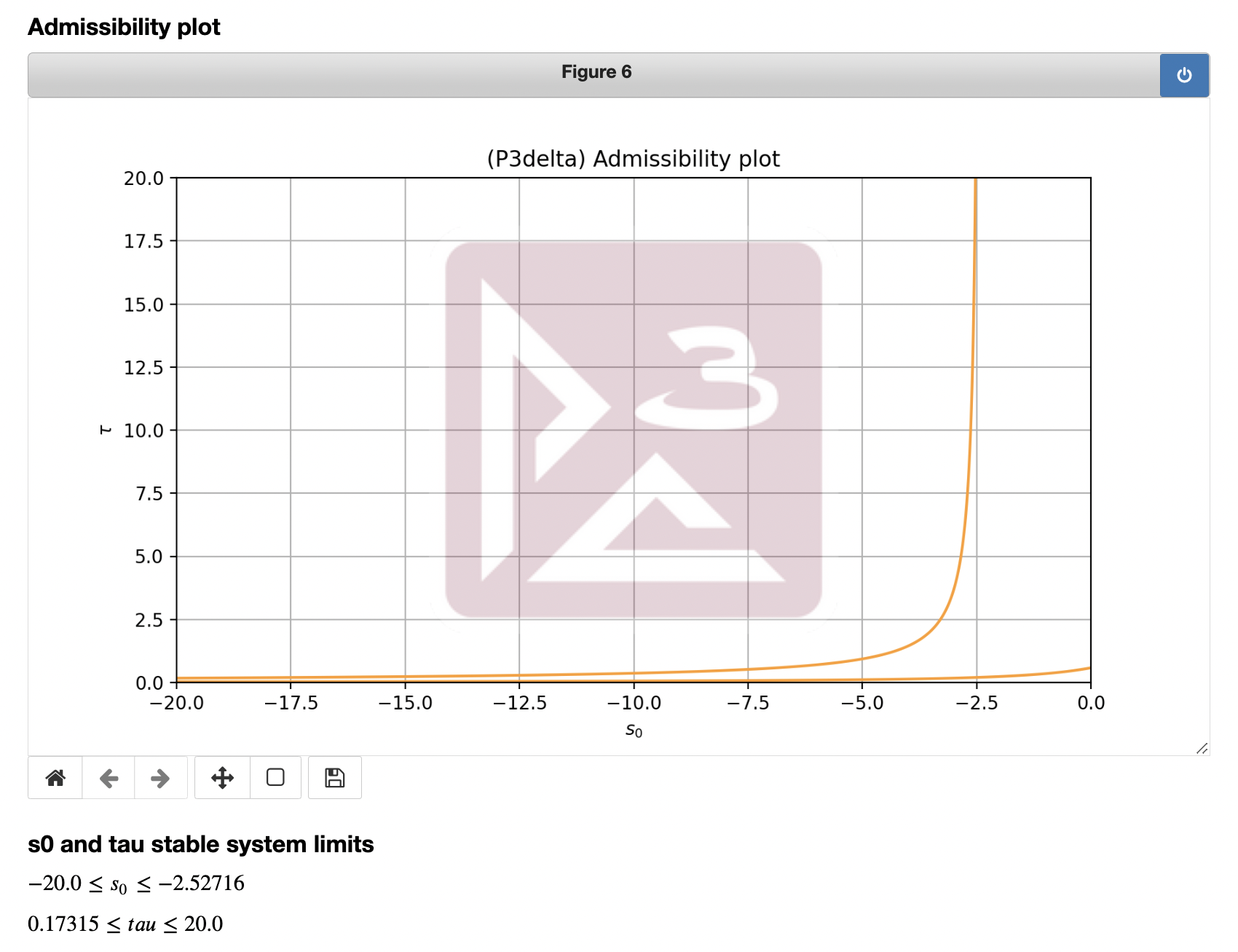
Figure 5: Admissibility plot for the inverted pendulum.

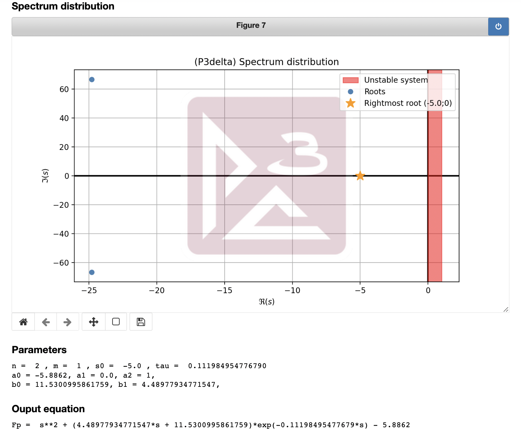
Figure 6: Computed values and spectrum distribution for the inverted pendulum.

By introducing the data corresponding to (7) into P3$\delta$ “Control-oriented MID” mode, we obtain the admissibility plot from Figure 5. Based on this plot, we decide to assign a root of multiplicity $3$ of (7) at $s_{0}=-5$. P3$\delta$ then gives the result shown in Figure 6. From the computed values of the coefficients shown in Figure 6, one deduces that the delay corresponding to $s_{0}=-5$ is $\tau\approx 0.112$ and the coefficients of (7) should be $\frac{K_{p}\ell}{2I}\approx 11.53$ and $\frac{K_{d}\ell}{2I}\approx 4.4898$, yielding the parameters $K_{p}\approx 192.16$ and $K_{d}\approx 74.83$.

3.3 Transonic flow in a wind tunnel

Consider now a wind tunnel in which a cold fluid is set to motion at high speed. The control of the velocity of such a fluid around an equilibrium state can be described by the system

$$\left\{\begin{aligned} \kappa m^{\prime}(t)+m(t)&=k\theta(t-\tau_{0}),\\ \theta^{\prime\prime}(t)+2\zeta\omega\theta^{\prime}(t)+\omega^{2}\theta(t)&=u(t),\end{aligned}\right.$$ (8)

where $m$ denotes the deviation of the Mach number of the fluid with respect to its equilibrium state, $\kappa$ and $k$ are constants depending on the characteristics of the fluid and the desired equilibrium state, $\theta$ is the angle of a guide vane driving the velocity of the fluid, $\tau_{0}>0$ is a delay depending only on the temperature of the fluid, $\zeta$ and $\omega$ are parameters of the dynamics of the guide vane angle, and $u$ is a control input. The above model comes from Armstrong and Tripp (1981) and its stabilization was previously discussed in Mazanti et al. (2021) under the assumption that one may choose $\zeta$ and $\omega$. We consider here a more realistic situation in which $\zeta$ and $\omega$ are fixed, and a feedback law of the form

$$u(t)=-\beta m(t-\tau_{1})-\alpha_{0}\theta(t-\tau_{0}-\tau_{1})-\alpha_{1}\theta^{\prime}(t-\tau_{0}-\tau_{1}),$$

where $\tau_{1}\geq 0$ is a new delay, which can be seen as a design parameter and should be at least equal to the delay for measuring $m$. For simplicity, we denote $\tau=\tau_{0}+\tau_{1}$. Inserting this control law into (8) and performing straightforward algebraic manipulations, one deduces that $\theta$ verifies the third-order differential equation

$$\textstyle\theta^{\prime\prime\prime}(t)+\left(2\zeta\omega+\frac{1}{\kappa}\right)\theta^{\prime\prime}(t)+\left(\omega^{2}+\frac{2\zeta\omega}{\kappa}\right)\theta^{\prime}(t)+\frac{\omega^{2}}{\kappa}\theta(t)\\ \textstyle{}+\alpha_{1}\theta^{\prime\prime}(t-\tau)+\left(\alpha_{0}+\frac{\alpha_{1}}{\kappa}\right)\theta^{\prime}(t-\tau)+\frac{\alpha_{0}+\beta k}{\kappa}\theta(t-\tau)=0,$$

and hence the closed-loop characteristic quasipolynomial $\Delta$ of (8) is

$$\begin{split}\textstyle\Delta(s)={}&\textstyle s^{3}+\left(2\zeta\omega+\frac{1}{\kappa}\right)s^{2}+\left(\omega^{2}+\frac{2\zeta\omega}{\kappa}\right)s+\frac{\omega^{2}}{\kappa}\\ &\textstyle{}+(\gamma_{2}s^{2}+\gamma_{1}s+\gamma_{0})e^{-s\sigma},\end{split}$$ (9)

where $\gamma_{2}=\alpha_{1}$, $\gamma_{1}=\alpha_{0}+\frac{\alpha_{1}}{\kappa}$, and $\gamma_{0}=\frac{\alpha_{0}+\beta k}{\kappa}$.

As a numerical application, we consider the linearization around the steady state with Mach number $0.84$ and air temperature $166$ K, in which case, as reported in Armstrong and Tripp (1981), the system parameters are $\kappa=1.964$ s, $k=-0.67036$ rad^-1, $\tau_{0}=0.33$ s, $\zeta=0.4368$, and $\omega=3.292$ rad s^-1. We can hence insert the known coefficients of (9) into P3$\delta$, as shown in Figure 7, and obtain the admissibility plot from Figure 8.

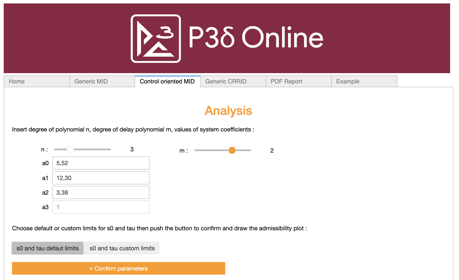
Figure 7: Data input for the transonic flow model.

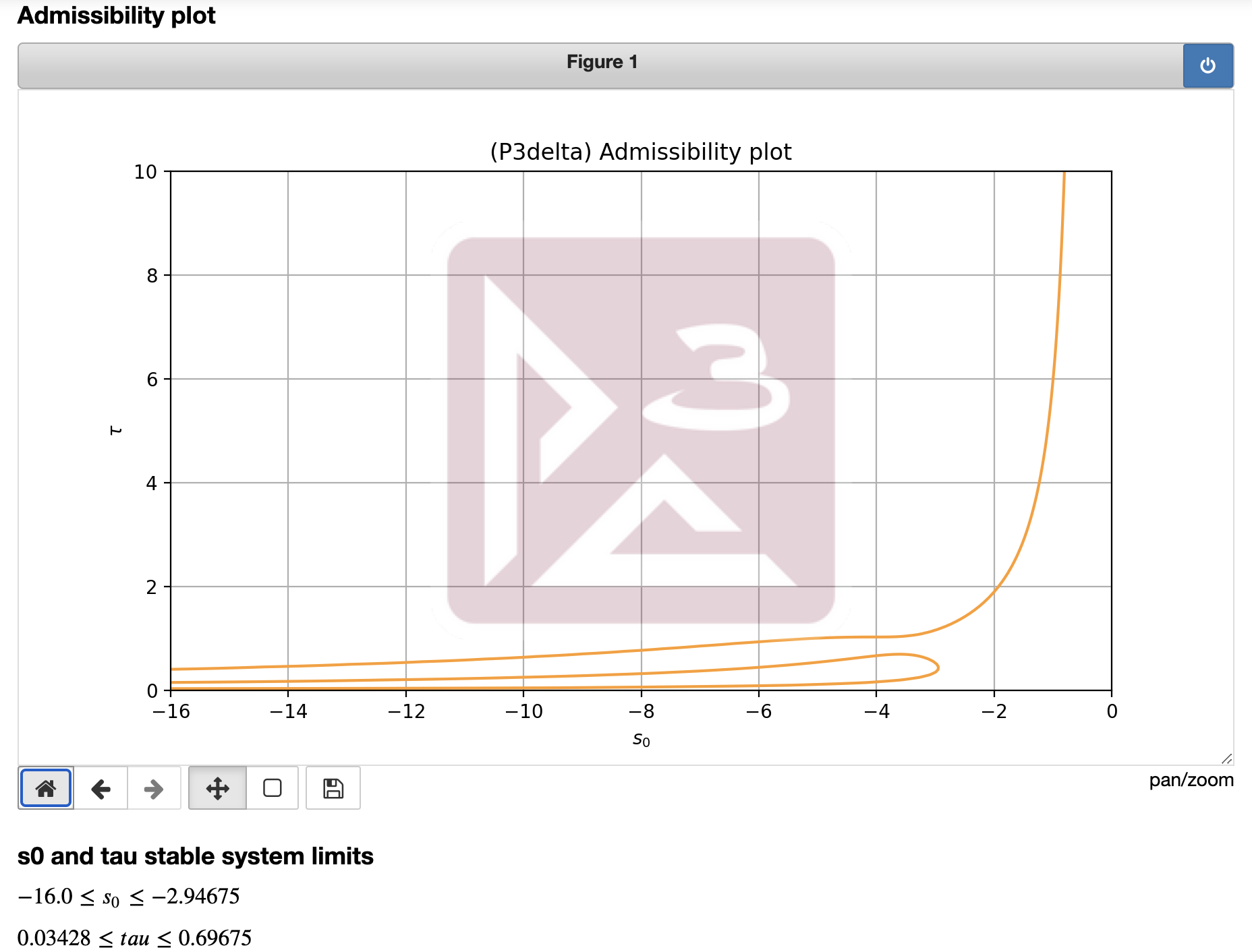
Figure 8: Admissibility plot for the transonic flow model.

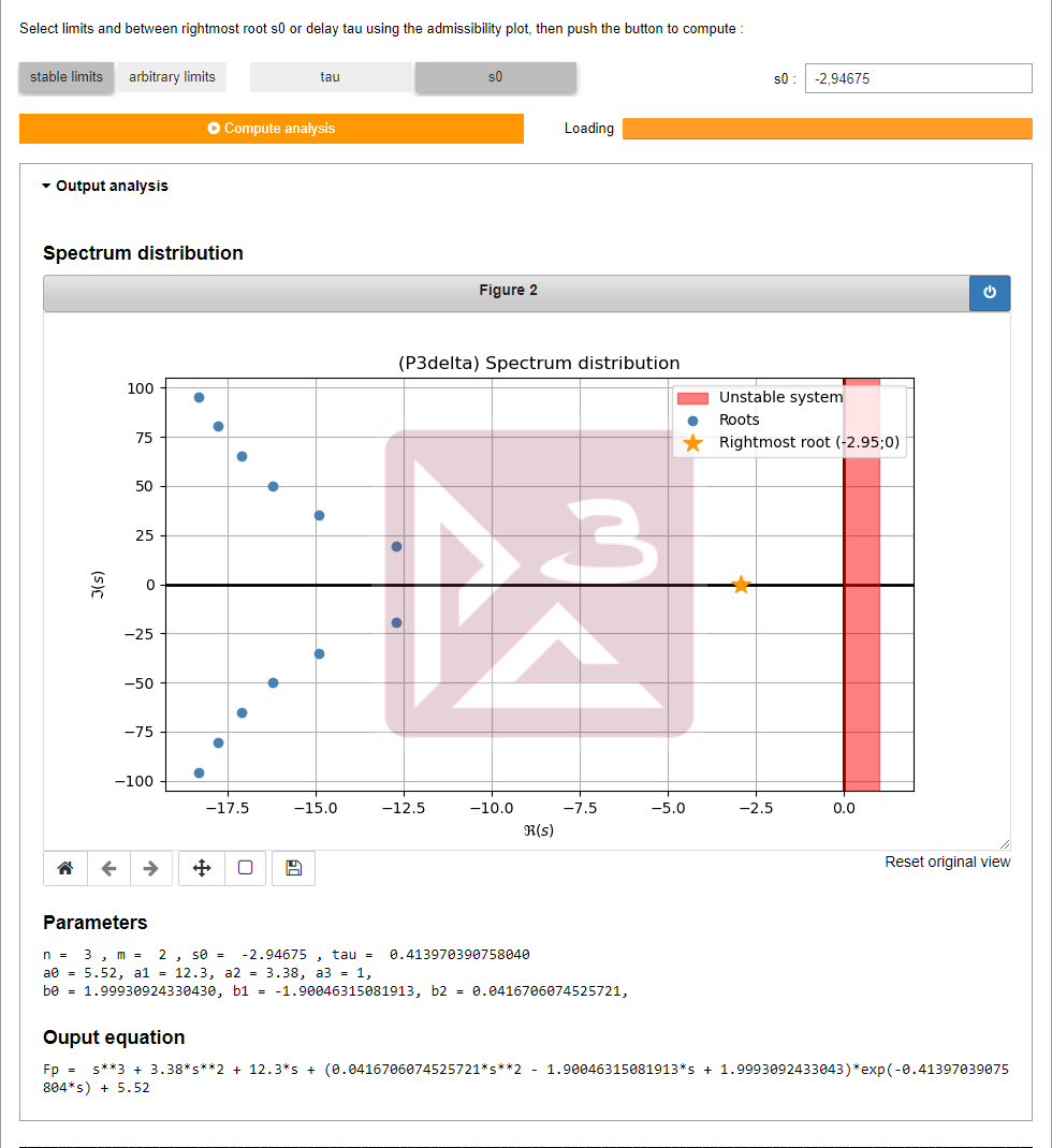
Figure 9: Computed values and spectrum distribution for the transonic flow model.

Based on Figure 8, we choose in this example $s_{0}=-2.94675$ as a root of multiplicity $5$ of the quasipolynomial $\Delta$, and P3$\delta$ provides the output shown in Figure 9. In particular, we deduce the numerical value $\tau\approx 0.4140$ s, yielding $\tau_{1}\approx 0.0840$ s, as well as $\gamma_{2}\approx 0.04167$, $\gamma_{1}\approx-1.9005$, and $\gamma_{0}\approx 1.9993$, yielding $\beta\approx-2.9908$, $\alpha_{0}\approx 1.9217$, and $\alpha_{1}\approx 0.04167$.

4 Concluding remarks and future work

By exploiting the properties of the MID and the CRRID, P3$\delta$ allows for the design of feedback control laws for real applications. The main novelty of the version discussed in the paper is the improvement of the graphic interface for the online version of the software. Inspired by the “Control-oriented MID” mode, the team is working on a “Control-oriented CRRID” mode. In addition, an executable version for macOS is currently under development.

References

- Amrane et al. (2018) Amrane, S., Bedouhene, F., Boussaada, I., and Niculescu, S.I. (2018). On qualitative properties of low-degree quasipolynomials: further remarks on the spectral abscissa and rightmost-roots assignment. Bull. Math. Soc. Sci. Math. Roumanie (N.S.), 61(109)(4), 361–381.
- Armstrong and Tripp (1981) Armstrong, E.S. and Tripp, J.S. (1981). An application of multivariable design techniques to the control of the National Transonic Facility. Technical Report 1887, NASA.
- Atay (1999) Atay, F.M. (1999). Balancing the inverted pendulum using position feedback. Appl. Math. Lett., 12(5), 51–56.
- Balogh et al. (2020) Balogh, T., Insperger, T., Boussaada, I., and Niculescu, S.I. (2020). Towards an MID-based delayed design for arbitrary-order dynamical systems with a mechanical application. IFAC-PapersOnLine, 53(2), 4375–4380. 21th IFAC World Congress.
- Balogh et al. (2022) Balogh, T., Boussaada, I., Insperger, T., and Niculescu, S.I. (2022). Conditions for stabilizability of time-delay systems with real-rooted plant. Internat. J. Robust Nonlinear Control, 32(6), 3206–3224.
- Bedouhene et al. (2020) Bedouhene, F., Boussaada, I., and Niculescu, S.I. (2020). Real spectral values coexistence and their effect on the stability of time-delay systems: Vandermonde matrices and exponential decay. Comptes Rendus. Mathématique, 358(9-10), 1011–1032.
- Benarab et al. (2020) Benarab, A., Boussaada, I., Trabelsi, K., Mazanti, G., and Bonnet, C. (2020). The MID property for a second-order neutral time-delay differential equation. In 2020 24th International Conference on System Theory, Control and Computing (ICSTCC), 202–207.
- Boussaada et al. (2022) Boussaada, I., Mazanti, G., and Niculescu, S.I. (2022). The generic multiplicity-induced-dominancy property from retarded to neutral delay-differential equations: When delay-systems characteristics meet the zeros of Kummer functions. Comptes Rendus. Math., 360, 349–369.
- Boussaada et al. (2020a) Boussaada, I., Mazanti, G., Niculescu, S.I., Huynh, J., Sim, F., and Thomas, M. (2020a). Partial pole placement via delay action: A python software for delayed feedback stabilizing design. In 2020 24th International Conference on System Theory, Control and Computing (ICSTCC), 196–201.
- Boussaada et al. (2021) Boussaada, I., Mazanti, G., Niculescu, S.I., Leclerc, A., Raj, J., and Perraudin, M. (2021). New features of P3delta software: Partial pole placement via delay action. IFAC-PapersOnLine, 54(18), 215–221. 16th IFAC Workshop on Time Delay Systems.
- Boussaada and Niculescu (2016a) Boussaada, I. and Niculescu, S.I. (2016a). Characterizing the codimension of zero singularities for time-delay systems: a link with Vandermonde and Birkhoff incidence matrices. Acta Appl. Math., 145, 47–88.
- Boussaada and Niculescu (2016b) Boussaada, I. and Niculescu, S.I. (2016b). Tracking the algebraic multiplicity of crossing imaginary roots for generic quasipolynomials: a Vandermonde-based approach. IEEE Trans. Automat. Control, 61(6), 1601–1606.
- Boussaada and Niculescu (2018) Boussaada, I. and Niculescu, S.I. (2018). On the dominancy of multiple spectral values for time-delay systems with applications. IFAC-PapersOnLine, 51(14), 55–60. 14th IFAC Workshop on Time Delay Systems.
- Boussaada et al. (2020b) Boussaada, I., Niculescu, S.I., El-Ati, A., Pérez-Ramos, R., and Trabelsi, K. (2020b). Multiplicity-induced-dominancy in parametric second-order delay differential equations: Analysis and application in control design. ESAIM Control Optim. Calc. Var., 26, Paper No. 57.
- Boussaada et al. (2018a) Boussaada, I., Niculescu, S.I., and Trabelsi, K. (2018a). Towards a decay rate assignment based design for time-delay systems with multiple spectral values. In Proceedings of the 23rd International Symposium on Mathematical Theory of Networks and Systems (MTNS), 864–871.
- Boussaada et al. (2018b) Boussaada, I., Tliba, S., Niculescu, S.I., Ünal, H.U., and Vyhlídal, T. (2018b). Further remarks on the effect of multiple spectral values on the dynamics of time-delay systems. Application to the control of a mechanical system. Linear Algebra Appl., 542, 589–604.
- Boussaada et al. (2016) Boussaada, I., Ünal, H.U., and Niculescu, S.I. (2016). Multiplicity and stable varieties of time-delay systems: A missing link. In Proceedings of the 22nd International Symposium on Mathematical Theory of Networks and Systems (MTNS), 188–194.
- Callender et al. (1936) Callender, A., Hartree, D.R., and Porter, A. (1936). Time-lag in a control system. Phil. Trans. Royal Soc. Series A, 235, 415–444.
- Gu et al. (2003) Gu, K., Kharitonov, V.L., and Chen, J. (2003). Stability of time-delay systems. Control Engineering. Birkhäuser Boston, Inc., Boston, MA.
- Hale and Verduyn Lunel (1993) Hale, J.K. and Verduyn Lunel, S.M. (1993). Introduction to functional differential equations. Springer-Verlag, New York.
- Hartree et al. (1937) Hartree, D.R., Porter, A., Callender, A., and Stevenson, A. (1937). Time-lag in a control system. II. Proc. Royal Soc. A, 161, 460–475.
- Ma et al. (2022) Ma, D., Boussaada, I., Chen, J., Bonnet, C., Niculescu, S.I., and Chen, J. (2022). PID control design for first-order delay systems via MID pole placement: Performance vs. robustness. Automatica, 137, 110102.
- Mazanti et al. (2020a) Mazanti, G., Boussaada, I., and Niculescu, S.I. (2020a). On qualitative properties of single-delay linear retarded differential equations: Characteristic roots of maximal multiplicity are necessarily dominant. IFAC-PapersOnLine, 53(2), 4345–4350. 21st IFAC WC.
- Mazanti et al. (2021) Mazanti, G., Boussaada, I., and Niculescu, S.I. (2021). Multiplicity-induced-dominancy for delay-differential equations of retarded type. J. Differential Equations, 286, 84–118.
- Mazanti et al. (2020b) Mazanti, G., Boussaada, I., Niculescu, S.I., and Vyhlídal, T. (2020b). Spectral dominance of complex roots for single-delay linear equations. IFAC-PapersOnLine, 53(2), 4357–4362. 21st IFAC World Congress.
- Michiels and Niculescu (2014) Michiels, W. and Niculescu, S.I. (2014). Stability, control, and computation for time-delay systems: An eigenvalue-based approach. SIAM, Philadelphia, PA, second edition.
- Molnar et al. (2021) Molnar, C.A., Balogh, T., Boussaada, I., and Insperger, T. (2021). Calculation of the critical delay for the double inverted pendulum. J. Vib. Control, 27(3-4), 356–364.
- Niculescu et al. (2010) Niculescu, S.I., Michiels, W., Gu, K., and Abdallah, C.T. (2010). Delay effects on output feedback control of dynamical systems. In F.M. Atay (ed.), Complex time-delay systems, 63–84. Springer, Berlin.
- Porter (1952) Porter, A. (1952). Introduction to servomechanisms. Wiley: London, 2nd edition.
- Sipahi et al. (2011) Sipahi, R., Niculescu, S.I., Abdallah, C.T., Michiels, W., and Gu, K. (2011). Stability and stabilization of systems with time delay: limitations and opportunities. IEEE Control Syst. Mag., 31(1), 38–65.
- Stépán (1989) Stépán, G. (1989). Retarded dynamical systems: stability and characteristic functions, volume 210 of Pitman Research Notes in Mathematics Series. Longman Scientific & Technical, Harlow.
- Suh and Bien (1979) Suh, I.H. and Bien, Z. (1979). Proportional minus delay controller. IEEE Trans. Automat. Control, 24(2), 370–372.