Rigidity of three-dimensional internal waves with constant vorticity

Abstract.

This paper studies the structural implications of constant vorticity for steady three-dimensional internal water waves. It is known that in many physical regimes, water waves beneath vacuum that have constant vorticity are necessarily two dimensional. The situation is more subtle for internal waves that traveling along the interface between two immiscible fluids. When the layers have the same density, there is a large class of explicit steady waves with constant vorticity that are three-dimensional in that the velocity field and pressure depend on one horizontal variable while the interface is an arbitrary function of the other. We prove the following rigidity result: every three-dimensional traveling internal wave with bounded velocity for which the vorticities in the upper and lower layers are nonzero, constant, and parallel must belong to this family. If the densities in each layer are distinct, then in fact the flow is fully two dimensional.

1. Introduction

Depth-varying currents are ubiquitous in the ocean. They can arise from wind-wave interaction, boundary layer effects along the seabed, or tides [25, 30, 17]. Waves riding on currents are essentially rotational, and the interaction of waves with non-uniform currents is described by the vorticity [27, 18]. So far most of the theoretical works on water waves with non-zero vorticity pertains to two-dimensional flows. The early 19th century work of Gerstner [9] furnished a family of exact solutions with a particular nontrivial vorticity distribution that becomes singular at the free surface of the highest wave. Much later, Dubreil-Jacotin [8] proved the existence of small-amplitude waves with a general vorticity distribution. After a surge of activity in this area over the last two decades, initiated by Constantin and Strauss [7], there is now a wealth of small- and large-amplitude existence results for water waves with vorticity; see [14] for a survey.

Despite these advances in the two-dimensional case, the understanding of three-dimensional rotational waves remains comparatively rudimentary. Currently, there are only two regimes in which existence is known: Lokharu, Seth, and Wahlén [20] have constructed small-amplitude three-dimensional waves with Beltrami-type flow, and Seth, Varholm, and Wahlén [28] obtained symmetric diamond waves with small vorticity. The first result is proved using a careful multi-parameter Lyapunov–Schmidt reduction, while the second involves a delicate fixed-point argument inspired by related problems in plasma physics.

Another body of important recent work concerns the rigidity of the governing equations: for certain types of vorticity, the solutions necessarily inherit symmetries of the domain. A number of authors have obtained results of this type for the Euler equations posed in a fixed domain. Moreover, it is known that finite-depth surface water waves beneath vacuum with non-zero constant vorticity are forced to be two dimensional with the vorticity vector pointing in the horizontal direction orthogonal to that of the wave propagation; see [6, 4, 21, 29] for flows beneath surface wave trains and surface solitary waves, [31] for general steady waves, and [22] for an extension to non-steady waves. Flows with geophysical effects are discussed in the survey article [24].

The present paper aims to investigate the structural ramifications of constant vorticity for steady three-dimensional internal water waves. An important feature of waves in the ocean is that the density is heterogeneous due to variations in temperature and salinity. Commonly, this situation is modeled as two immiscible, superposed layers of constant density fluids. The interface dividing these regions is a free boundary along which internal waves can travel. Similar to surface waves, the theoretical study on internal waves has been conducted almost exclusively in two dimensions; see [14, Section 7]. To the authors’ knowledge the only rigorous existence result for genuinely three-dimensional steady internal waves is due to Nilsson [26], where the flow is assumed to be layer-wise irrotational. It is then natural to ask whether the rigidity of surface water waves with constant vorticity has an internal wave counterpart. As the latter system has many additional parameters, in principle we might expect it to support a greater variety of flows. For instance, it can be shown if the vorticity is constant in each layer, then it must be horizontal, but its direction need not be the same in each layer. On the other hand, if the vorticity vectors are parallel and nonvanishing, we are able to prove a rigidity result that completely characterizes the possible flow patterns.

1.1. Formulation

Consider a three-dimensional traveling wave moving along the interface dividing two immiscible fluids of finite depth and under the influence of gravity. Fix a Cartesian coordinate system $(x,y,z)$, where $z$ is the vertical direction and the wave propagates in the $xy$-plane. The fluids are bounded above and below by rigid walls at heights $z=-h_{1}$ and $z=h_{2}$, for $h_{1},h_{2}>0$. Adopting a frame of reference moving with the wave renders the system time independent. Suppose then that the interface between the layers is given by the graph of a $C^{1}$ function $\eta=\eta(x,y)$. The fluid domain is thus $\Omega:=\Omega_{1}\cup\Omega_{2}$, where the upper layer $\Omega_{2}$ and lower layer $\Omega_{1}$ take the form

$$\Omega_{1} :=\left\{(x,y,z)\in\mathbb{R}^{3}:-h_{1}<z<\eta(x,y)\right\}$$

$$\Omega_{2} :=\left\{(x,y,z)\in\mathbb{R}^{3}:\eta(x,y)<z<h_{2}\right\}.$$

See Figure 1 for an illustration.

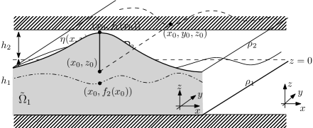
Figure 1. The two-fluid system.

For water waves, it is physically reasonable to model the flow in each region as inviscid and incompressible with constant densities $\rho_{1},\rho_{2}>0$. The motion in $\Omega_{i}$ is described by the (relative) velocity field $\boldsymbol{u}_{i}:=\left(u_{i},v_{i},w_{i}\right)$ and pressure $P_{i}$. In the bulk, we impose the steady incompressible Euler equations:

(1.1a) $$\rho_{i}(\boldsymbol{u}_{i}\cdot\nabla)\boldsymbol{u}_{i} =-\nabla P_{i}+\rho_{i}\boldsymbol{g},$$

(1.1b) $$\nabla\cdot\boldsymbol{u}_{i} =0,$$

where $$\boldsymbol{g}:=(0,0,-g)$$ is the (constant) gravitational acceleration vector. The first of these mandates the conservation of momentum, while the second is the incompressibility condition. The boundary conditions at the interface are the continuity of normal velocity and pressure:

(1.1c) $$u_{i}\eta_{x}+v_{i}\eta_{y} =w_{i}\quad\text{on }z=\eta(x,y),$$

(1.1d) $$P_{1} =P_{2}\quad\text{on }z=\eta(x,y).$$

On the upper and lower rigid boundaries, the kinematic boundary conditions are

(1.1e) $$w_{1} =0 \textrm{on }z=-h_{1}$$

$$w_{2} =0 \textrm{on }z=h_{2}.$$

These say simply that the velocity field is tangential to the rigid walls. Throughout this paper, we consider classical solutions for which $\boldsymbol{u}_{i}\in C^{1}(\overline{\Omega_{i}};\mathbb{R}^{3})$, $P_{i}\in C^{1}(\overline{\Omega_{i}})$, and $\eta\in C^{1}(\mathbb{R}^{2})$. In order to ensure there is a positive separation between the interface and the walls, we further assume that $-h_{1}<\inf{\eta}$ and $\sup{\eta}<h_{2}$.

Recall that the vorticity in the layer $\Omega_{i}$ is defined to be the vector field

(1.2) $$\boldsymbol{\omega}_{i}:=\nabla\times\boldsymbol{u}_{i}=(\partial_{y}w_{i}-\partial_{z}v_{i},\,\partial_{z}u_{i}-\partial_{x}w_{i},\,\partial_{x}v_{i}-\partial_{y}u_{i}).$$

Taking the curl of the momentum equation (1.1a), we find that each $\boldsymbol{\omega}_{i}$ satisfies the so-called steady vorticity equation

(1.3) $$(\boldsymbol{u}_{i}\cdot\nabla)\boldsymbol{\omega}_{i}=(\boldsymbol{\omega}_{i}\cdot\nabla)\boldsymbol{u}_{i}\qquad\textrm{in }\Omega_{i}.$$

Suppose now that the vorticity in each layer is a nonzero constant

(1.4) $$\boldsymbol{\omega}_{i}=(\alpha_{i},\beta_{i},\gamma_{i})\qquad\textrm{for }i=1,2.$$

Then the advection term on the left-hand side of (1.3) vanishes identically, while the vortex stretching term on the right-hand side becomes a constant directional derivative of $\boldsymbol{u}$:

(1.5) $$(\boldsymbol{\omega}_{i}\cdot\nabla)\boldsymbol{u}_{i}=0\qquad\textrm{in }\Omega_{i}.$$

Thus, the velocity $\boldsymbol{u}_{i}$ is constant in the direction of $\boldsymbol{\omega}_{i}$. As (1.1) is invariant under rotation about the $z$-axis, we can without loss of generality assume that $\boldsymbol{\omega}_{2}=(0,\beta_{2},\gamma_{2})$, that is, the vorticity of the upper fluid lies in the $yz$-plane.

From the vector identity

$$(\boldsymbol{u}\cdot\nabla)\boldsymbol{u}+\boldsymbol{u}\times\boldsymbol{\omega}=(\nabla\cdot\boldsymbol{u})\boldsymbol{u}+\frac{1}{2}\nabla(|\boldsymbol{u}|^{2}),$$

one can rewrite (1.1a) as

(1.6) $$\boldsymbol{u}_{i}\times\boldsymbol{\omega}_{i}=\nabla H_{i}$$

where

(1.7) $$H_{i}:=\frac{1}{2}|\boldsymbol{u}_{i}|^{2}+\frac{P_{i}}{\rho_{i}}+gz$$

is called the Bernoulli function. From (1.6) we see that $H_{i}$ is constant along the vortex lines.

1.2. Main results

Our first theorem imposes a dimensionality constraint on the vorticity: if $\boldsymbol{u}_{1}$ and $\boldsymbol{u}_{2}$ are uniformly bounded, then both vorticity vectors $\boldsymbol{\omega}_{1}$ and $\boldsymbol{\omega}_{2}$ are necessarily two-dimensional and lie in the $xy$-plane. A result of this type was first proved by Wahlén [31] for steady gravity and capillary-gravity water waves beneath vacuum. Martin [22] later showed the same holds for the time-dependent case. Adapting Wahlén’s argument to the two-layer case requires some nontrivial new analysis due to the more complicated behavior at the interface. Ultimately, we obtain the following.

Theorem 1.1.

Consider a solution to the internal wave problem (1.1) such that $\|\boldsymbol{u}_{1}\|_{C^{0}},\|\boldsymbol{u}_{2}\|_{C^{0}}<\infty$ and $\boldsymbol{\omega}_{1}$ and $\boldsymbol{\omega}_{2}$ are nonzero constant vectors. Then necessarily the third components of $\boldsymbol{\omega}_{1}$ and $\boldsymbol{\omega}_{2}$ both vanish.

Next, we consider the structure of the velocity field and free surface profile. Under remarkably general conditions, Wahlén [31] proves that for a gravity wave beneath vacuum, if the vorticity is constant, then the flow must be entirely two dimensional: $\boldsymbol{u}_{i}$ lies in the $xz$-plane and depends only on $(x,z)$, while $\eta=\eta(x)$. In other words, genuinely three-dimensional steady surface gravity water waves with non-zero constant vorticity do not exist. Wahlén also proves the same holds for capillary-gravity waves provided the velocity field and free surface profile are uniformly bounded in $C^{1}$, and a Taylor sign condition on the pressure holds. Earlier work by Constantin [4], Constantin and Kartashova [6], and Martin [21] obtain analogous results for gravity and capillary-gravity waves under the more restrictive assumption that $\eta$ is periodic, while Martin treats time-dependent [22] and viscous waves [23] again with a Taylor sign condition; see also the survey in [24]. The moral of this body of work is that in order to find genuinely three-dimensional steady rotational waves beneath vacuum, one must allow for a more complicated vorticity distribution.

However, constant vorticity internal waves are not obliged to be two dimensional. Indeed, a little thought readily leads us to a profusion of explicit three-dimensional solutions to (1.1). Assume that we are in the the Boussinesq setting where $\rho_{1}=\rho_{2}$. Then, taking

(1.8) $$\boldsymbol{u}_{i}=(\beta_{i}z+k_{i},0,0)\quad\textrm{for }i=1,2,\qquad\eta=H(y)$$

gives a steady wave for any $H\in C^{1}(\mathbb{R};(-h_{1},h_{2}))$. Note that the corresponding vorticity vectors $\boldsymbol{\omega}_{i}=(0,\beta_{i},0)$ are parallel. We can visualize (1.8) as two shear flows defined in $\overline{\Omega}$, which when $\rho_{1}=\rho_{2}$ will have the same (hydrostatic) pressure. Any streamline in the $xz$-plane can be viewed as a material interface above which we have the first fluid and below the second. When $v_{1},v_{2}\equiv 0$, we can smoothly vary which streamline is the interface as we change $y$, permitting there to be three-dimensional structure. Essentially, the difference between the situation here and the one-layer case lies in the dynamic condition (1.1d). When the fluid is bounded above by vacuum, the pressure must be constant along the interface, whereas for internal waves it need only be continuous.

Members of the family of solutions (1.8) can be thought of as trivially three-dimensional shear flows when $\eta_{y}\not\equiv 0$. Our main theorem shows that they are in fact the only possible configuration for three-dimensional waves with constant parallel vorticity and bounded velocity.

Theorem 1.2 (Rigidity).

Every solution of the internal wave problem (1.1) for which

1. $\boldsymbol{\omega}_{1}$ and $\boldsymbol{\omega}_{2}$ are constant, parallel, and nonzero, and

2. $\|\boldsymbol{u}_{1}\|_{C^{0}}$, $\|\boldsymbol{u}_{2}\|_{C^{0}}<\infty$,

is either a trivially three-dimensional shear flow of the form (1.8) or two dimensional. If $\rho_{1}\neq\rho_{2}$, then the wave is necessarily two dimensional.

One can interpret this theorem as the statement that the solutions to (1.1) inherit the symmetry of the channel domain in which the problem is posed. Related rigidity results for the two-dimensional Euler equations have been obtained by Hamel and Nadirashvili [11, 12], who prove that all solutions in a strip, half plane, or the whole plane with no stagnation points are shear flows (that is, the vertical velocity vanishes identically and the horizontal velocity depends only on $z$). Under the same no-stagnation assumption, these authors also find that steady Euler configurations confined to circular domains must be radially symmetric [13]. Allowing the presence of stagnation points, Gómez-Serrano, Park, Shi, and Yao [10] show that smooth stationary solution with compactly supported and nonnegative vorticity must be radial. In Theorem 1.2 we avoid making any restrictions on the velocity beyond boundedness, though we only treat the constant vorticity case. Notably, as in [31], we make no a priori assumptions on the far-field behavior of the wave. Thus in the non-Boussinesq case, nontrivial solitary waves, periodic waves, fronts — and all other more exotic waveforms — are excluded all at once. We also mention that it is possible to rule out capillary-gravity internal waves through arguments similar to the one-fluid regime; see Theorem 4.1.

The idea of the proof can be explained as follows. Thanks to Theorem 1.1, when $\boldsymbol{\omega}_{1}$ and $\boldsymbol{\omega}_{2}$ are parallel, the velocity fields are two-dimensional: $\boldsymbol{u}_{i}=(u_{i}(x,z),V_{i},w_{i}(x,z))$ where $V_{i}$ are constants. The same also holds for the pressures, but a priori $\eta$ may depend on both $(x,y)$. If the interface is not independent of $y$, then the projections $\tilde{\Omega}_{i}$ of $\Omega_{i}$ into the $xz$-plane will have non-empty intersection with non-empty interior, and on that set we have two solutions of the two-dimensional Euler equations. Because each point in $\tilde{\Omega}_{1}\cap\tilde{\Omega}_{2}$ corresponds to one or more points on the interface, the dynamic condition applies throughout. The key insight of Wahlén is that, for waves beneath vacuum, this forces the pressure to be constant, and hence by analyticity, it is constant throughout the fluid. As this is not possible, he concludes that for surface waves, the interface must be flat in $y$. For internal waves, however, the dynamic condition tells us instead that there exists a pressure $P=P(x,z)$ that is real analytic on $\tilde{\Omega}_{1}\cup\tilde{\Omega}_{2}$ and whose restriction to $\tilde{\Omega}_{1}$ is $P_{1}$ and whose restriction to $\tilde{\Omega}_{2}$ is $P_{2}$.

The central question therefore turns to one of uniqueness of steady solutions of the two-dimensional Euler equations with a prescribed pressure, but allowing for potentially different densities and different constant vorticities. We have in addition that the kinematic condition (1.1c) holds on the intersection region, which forces a relation between the slopes of the two velocity fields there. Through a novel but elementary argument, we prove that the streamlines (integral curves) of the vector fields $(u_{1},w_{1})$ and $(u_{2},w_{2})$ coincide on $\tilde{\Omega}_{1}\cap\tilde{\Omega}_{2}$. Finally, from the real analyticity of the velocity and pressure and Liouville’s theorem, we are ultimately able to conclude that the pressure must be hydrostatic, and thus the wave is of the form (1.8).

2. Dimension reduction for the vorticity

This section is devoted to the proof of Theorem 1.1 on the two-dimensionality of the vorticity. As mentioned above, it is based on the corresponding work of Wahlén in [31]. The main point is that this argument relies on the structure of the velocity field near the rigid walls, which is not substantially different in the two-fluid setting.

A key observation, both for the present section and the next, is that each component of the velocity is harmonic:

(2.1) $$\Delta u_{i}=\Delta v_{i}=\Delta w_{i}=0\qquad\textrm{in }\Omega_{i}.$$

This follows simply by taking the curl of equation (1.2) and using incompressibility (1.1b). As just one important consequence, $u_{i}$, $v_{i}$, and $w_{i}$ are all real-analytic functions. Taking the divergence of the momentum equation (1.1a), we likewise find that the pressure $P_{i}$ solves a Poisson equation with real-analytic forcing, and hence it too is real analytic. These facts will be crucial to our analysis at several points. In particular, they provide a means to globalize identities that hold on open subsets to the entirety of the fluid domain.

Proof of Theorem 1.1.

Seeking a contradiction, suppose that one of $\gamma_{i}$ is not zero, say, $\gamma_{1}\neq 0$; the argument for the other case $\gamma_{2}\neq 0$ can be treated the same way. Then from the third component of the vorticity equation (1.5) we see that $w_{1}$ is constant in the direction of $\boldsymbol{\omega}_{1}$, which is transverse to the lower boundary at $z=-h_{1}$. From the kinematic condition (1.1e), it follows that $w_{1}$ vanishes identically on the open neighborhood $\mathcal{N}:=\{(x,y,z):-h_{1}<z<\inf\eta\}$ of the bed. As it is real analytic, this forces

$$w_{1}\equiv 0\quad\text{in }\ \Omega_{1}.$$

Reconciling this with (1.4), (1.1b) and (1.1a), we then have

(2.2) $$\partial_{z}u_{1}=\beta_{1},\quad\partial_{z}v_{1}=-\alpha_{1},$$

(2.3) $$\partial_{x}u_{1}+\partial_{y}v_{1}=0,$$

(2.4) $$\partial_{z}P_{1}=-\rho_{1}g$$

in $\Omega_{1}$. By integrating (2.2), we infer that

(2.5) $$u_{1}=\bar{u}_{1}(x,y)+\beta_{1}z,\qquad v_{1}=\bar{v}_{1}(x,y)-\alpha_{1}z,$$

in $\mathcal{N}$ for some functions $\bar{u}_{1}$ and $\bar{v}_{1}$. The reduced incompressibility condition (2.3) then implies that

$$\partial_{x}\bar{u}_{1}+\partial_{y}\bar{v}_{1}=0,$$

which ensures the existence of a reduced stream function $\bar{\psi}_{1}=\bar{\psi}_{1}(x,y)$ defined on $\mathcal{N}$ such that $\nabla^{\perp}\bar{\psi}_{1}=(-\partial_{z}\bar{\psi},\partial_{x}\bar{\psi})=(\bar{u}_{1},\bar{v}_{1})$. From the horizontal momentum equations (1.1a) and the form of the pressure obtained in (2.4), we see in $\mathcal{N}$, $\bar{\psi}_{1}$ satisfies

(2.6) $$\left\{\begin{split}\beta_{1}\partial_{x}\partial_{y}\bar{\psi}_{1}-\alpha_{1}\partial_{y}^{2}\bar{\psi}_{1}&=0\\ -\beta_{1}\partial_{x}^{2}\bar{\psi}_{1}+\alpha_{1}\partial_{x}\partial_{y}\bar{\psi}_{1}&=0\\ \Delta\bar{\psi}_{1}+\gamma_{1}&=0\end{split}\right.\qquad\textrm{in }\mathcal{N}.$$

We consider two cases.

Case 1: $\alpha_{1}^{2}+\beta_{1}^{2}=0$. From (2.2) and (1.4) it follows that

(2.7) $$\partial_{z}u_{1}=\partial_{z}v_{1}=0,\qquad\partial_{x}v_{1}-\partial_{y}u_{1}=\gamma_{1}.$$

We also find from (2.5) and (2.1) that in the neighborhood $\mathcal{N}$, $u_{1}=\bar{u}_{1}$ and $v_{1}=\bar{v}_{1}$ are harmonic functions with domain $\mathbb{R}^{2}$. The boundedness of $\boldsymbol{u}_{1}$, and thus the boundedness of $(\bar{u}_{1},\bar{v}_{1})$, allows one to appeal to the Liouville theorem for harmonic functions to conclude that $u_{1}$ and $v_{1}$ are constants. However this contradicts that fact that $\gamma_{1}\neq 0$.

Case 2: $\alpha_{1}^{2}+\beta_{1}^{2}\neq 0$. In this case, direct computation from (2.6) yields that the second-order derivatives of $\bar{\psi}_{1}$ are all constant:

(2.8) $$\partial_{x}^{2}\bar{\psi}_{1}=-{\alpha_{1}^{2}\gamma_{1}\over\alpha_{1}^{2}+\beta_{1}^{2}}=:A_{1},\quad\partial_{x}\partial_{y}\bar{\psi}_{1}=-{\alpha_{1}\beta_{1}\gamma_{1}\over\alpha_{1}^{2}+\beta_{1}^{2}}=:B_{1},\quad\partial_{y}^{2}\bar{\psi}_{1}=-{\beta_{1}^{2}\gamma_{1}\over\alpha_{1}^{2}+\beta_{1}^{2}}=:C_{1},$$

from which one can solve for $\bar{u}_{1}$ and $\bar{v}_{1}$

$$\bar{u}_{1}=B_{1}x+C_{1}y+a_{1},\qquad\bar{v}_{1}=-A_{1}x-B_{1}y+b_{1}$$

for some constants $a_{1}$ and $b_{1}$. Thus

(2.9) $$u_{1}=B_{1}x+C_{1}y+\beta_{1}z+a_{1},\qquad v_{1}=-A_{1}x-B_{1}y-\alpha_{1}z+b_{1}.$$

Again boundedness of $\boldsymbol{u}_{1}$ forces $A_{1}=B_{1}=C_{1}=0$, leading to $\alpha_{1}=\beta_{1}=0$, a contradiction. ∎

3. Rigidity of internal waves

The purpose of this section is to prove the rigidity result in Theorem 1.2, characterizing three-dimensional internal waves with constant vorticity. Recall that we have, without loss of generality, chosen axes so that $\boldsymbol{\omega}_{2}$ lies in the $xz$-plane. Theorem 1.1 then guarantees that the vorticity in each layer takes the form

(3.1) $$\boldsymbol{\omega}_{1}=(\alpha_{1},\beta_{1},0),\qquad\boldsymbol{\omega}_{2}=(0,\beta_{2},0).$$

Note that the assumption $\boldsymbol{\omega}_{1}$ and $\boldsymbol{\omega}_{2}$ are parallel is equivalent to $\alpha_{1}=0$. More generally, though, the particularly simple form of $\boldsymbol{\omega}_{2}$ allows one us further characterize the flow pattern in the upper layer.

Lemma 3.1.

Let the assumptions of Theorem 1.1 hold. Then, $\boldsymbol{u}_{2}$ and $P_{2}$ are independent of $y$, and $v_{2}$ is constant. Likewise, $\boldsymbol{u}_{1}$ and $P_{1}$ are constant along lines parallel to $\boldsymbol{\omega}_{1}$, while $\alpha_{1}u_{1}+\beta_{1}v_{1}$ is constant.

Proof.

We will only present the argument for the upper fluid as the lower fluid follows through essentially the same reasoning. From (3.1), (1.4) and (1.5) it follows that

$$\partial_{y}u_{2}=\partial_{y}v_{2}=\partial_{y}w_{2}=0,\qquad\partial_{x}v_{2}=\partial_{z}v_{2}=0.$$

In particular, $\nabla v_{2}=0$, and thus $v_{2}$ is a constant throughout $\Omega_{2}$. The momentum equation in $y$-directional momentum equation then becomes

$$\partial_{y}P_{2}=0\qquad\textrm{in }\Omega_{2}.$$

Following the argument as in [31, Lemma 3] using the real analyticity of $P_{2}$ we can show that $P_{2}$ is independent of $y$ in the upper fluid layer $\Omega_{2}$. In fact we see that $P_{2}$ is independent of $y$ in a region sufficiently close to the top boundary $\{z=h_{2}\}$. Therefore for any $y_{1}\neq y_{2}$, there exists a minimal $z_{*}\leq h_{2}$ such that

$$P_{2}(x,y_{1},z)=P_{2}(x,y_{2},z)\quad\text{for}\quad z_{*}\leq z\leq h_{2}.$$

Clearly we know that $z_{*}\geq\max\{\eta(x,y_{1}),\eta(x,y_{2})\}$. Using the real analyticity of $z\mapsto P_{2}(x,y_{1},z)-P_{2}(x,y_{2},z)$ we see that $z_{*}=\max\{\eta(x,y_{1}),\eta(x,y_{2})\}$, which indicates that $P_{2}$ is independent of $y$ in $\Omega_{2}$. The result for $(u_{2},w_{2})$ follows in a similar way. ∎

Let us now proceed to the proof of the main result.

Proof of Theorem 1.2.

Thanks to Lemma 3.1 and the assumption that $\boldsymbol{\omega}_{1}$ and $\boldsymbol{\omega}_{2}$ are parallel and non-vanishing, we have that $v_{1}$ and $v_{2}$ are constants; let them be denoted $V_{1}$ and $V_{2}$, respectively. Moreover, $\boldsymbol{u}_{1},P_{1},\boldsymbol{u}_{2}$, and $P_{2}$ are independent of $y$, so we can write

$$\boldsymbol{u}_{1}(x,y,z) =\tilde{\boldsymbol{u}}_{1}(x,z), \quad P_{1}(x,y,z) =\tilde{P}_{1}(x,z),$$

$$\boldsymbol{u}_{2}(x,y,z) =\tilde{\boldsymbol{u}}_{2}(x,z), \quad P_{2}(x,y,z) =\tilde{P}_{2}(x,z),$$

where $\tilde{\boldsymbol{u}}_{i}$ and $\tilde{P}_{i}$ are defined on the projection

(3.2) $$\tilde{\Omega}_{i}:=\left\{(x,z):\ (x,y,z)\in\Omega_{i}\text{ for some }y\in\mathbb{R}\right\},$$

of $\Omega_{i}$ on the $xz$-plane, for $i=1,2$. It is easy to see that in fact

(3.3) $$\tilde{\Omega}_{1}=\left\{(x,z):\ -h_{1}<z<f_{1}(x)\right\},\quad\tilde{\Omega}_{2}=\left\{(x,z):\ f_{2}(x)<z<h_{2}\right\},$$

where

$$f_{1}(x):=\sup_{y\in\mathbb{R}}\eta(x,y),\quad\text{and}\quad f_{2}(x):=\inf_{y\in\mathbb{R}}\eta(x,y).$$

By definition $f_{2}(x)\leq f_{1}(x)$. The boundedness of $\eta$ implies that $-h_{1}<f_{1}(x)\leq h_{2}$ and $-h_{1}\leq f_{2}(x)<h_{2}$. It is elementary that $f_{1}$ is then lower semicontinuous while $f_{2}$ is upper semicontinuous. The projected planes $\tilde{\Omega}_{i}$ are both open and connected subsets of $\mathbb{R}^{2}$, for $i=1,2$.

Arguing by contrapositive, suppose that $\eta_{y}\not\equiv 0$. Then $\tilde{\Omega}_{1}\cap\tilde{\Omega}_{2}\neq\emptyset$ and there exists some point $(x_{0},y_{0})$ such that $z_{0}:=\eta(x_{0},y_{0})\in(f_{2}(x_{0}),f_{1}(x_{0}))$. The dynamic boundary condition (1.1d) yields

$$\tilde{P}_{1}(x_{0},z_{0})=\tilde{P}_{2}(x_{0},z_{0}).$$

A continuity argument implies that for each $z$ between $z_{0}$ and $f_{1}(x_{0})$ there exists some $y(z)$ such that $z=\eta(x_{0},y(z))$. Therefore on the line segment joining $(x_{0},z_{0})$ and $(x_{0},f_{1}(x_{0}))$ we have

$$\tilde{P}_{1}(x_{0},z)=\tilde{P}_{2}(x_{0},z).$$

See Figure 2.

Figure 2. Projection to $\tilde{\Omega}_{1}$.

Now from the lower semicontinuity of $f_{1}$ and the upper semicontinuity of $f_{2}$ we know that for $x$ sufficiently close to $x_{0}$ it holds that $f_{2}(x)<\eta(x,y_{0})<f_{1}(x)$. Repeating the previous argument it follows that there exists an open subset of $\tilde{\Omega}_{1}$ in which $\tilde{P}_{1}(x,z)=\tilde{P}_{2}(x,z)$. The analyticity of $\tilde{P}_{i}$ then forces $\tilde{P}_{1}=\tilde{P}_{2}$ on $\tilde{\Omega}_{1}\cap\tilde{\Omega}_{2}$, and thus $\tilde{P}_{1}$ and $\tilde{P}_{2}$ are analytic extensions of each other in the entire strip $\tilde{\Omega}:=\left\{(x,z):\ -h_{1}<z<h_{2}\right\}$.

Recall that we say the pressure in $\tilde{\Omega}_{i}$ is hydrostatic provided $\nabla(\tilde{P}_{i}+\rho_{i}z)$ vanishes identically. Suppose that either $\tilde{P}_{1}$ or $\tilde{P}_{2}$ is hydrostatic. Then uniqueness of the analytic extension implies both are hydrostatic and hence $\rho_{1}=\rho_{2}$. The incompressibility of $\tilde{\boldsymbol{u}}_{1}$ and $\tilde{\boldsymbol{u}}_{2}$ permit us to define stream functions $\tilde{\psi}_{i}$ by $\nabla^{\perp}\tilde{\psi}_{i}:=(\tilde{u}_{i},\tilde{w}_{i})$. The Bernoulli equation (1.6) now reads

$$\beta_{i}(-\tilde{w}_{i},0,\tilde{u}_{i})=\nabla\left[\frac{1}{2}({\tilde{u}_{i}}^{2}+V_{i}^{2}+{\tilde{w}_{i}}^{2})\right]\quad\textrm{in }\Omega_{i},$$

which in turn leads to

$$\frac{1}{2}\left(\tilde{u}_{i}^{2}+\tilde{w}_{i}^{2}\right)-\beta_{i}\tilde{\psi}_{i}=Q_{i}\quad\textrm{in }\tilde{\Omega}_{i}$$

for some constant $Q_{i}$. On the bed, $\tilde{w}_{1}\equiv 0$ and $\tilde{\psi}_{1}$ is constant, and so $\tilde{u}_{1}$ is likewise constant there. Thus,

$$\tilde{w}_{1z}=\tilde{u}_{1x}=0\qquad\textrm{on }\{z=-h_{1}\},$$

and, because $\tilde{w}$ is harmonic, it must therefore be that $\tilde{w}_{1}\equiv 0$ in $\tilde{\Omega}_{1}$. The same argument applied on the lid shows that $\tilde{w}_{2}\equiv 0$ in $\tilde{\Omega}_{2}$. Incompressibility then implies that $\tilde{u}_{1}=U_{1}(z)$ and $\tilde{u}_{2}=U_{2}(z)$, meaning we have a shear flow. The constant vorticity then forces $\tilde{u}_{i}=\beta_{i}z+k_{i}$ as in (1.8).

Evaluating the kinematic condition using this fact gives

$$(\beta_{1}\eta+k_{1})\eta_{x}+V_{1}\eta_{y}=0\qquad\textrm{for all }(x,y)\in\mathbb{R}^{2}.$$

If $V_{1}\neq 0$, this is Burgers’ equation with $y$ playing the role of the evolution variable. Because the only global classical solutions are constants, this forces the interface to be perfectly flat. On the other hand, if $V_{1}=0$, we can simply integrate the equation in $x$ to see that $\eta(\,\cdot\,,y)$ is likewise constant. In either case, then, the wave is completely shear with no variation in the $x$-direction.

As the converse of these inferences is obviously true, the conclusions of the previous two paragraphs can be stated succinctly as:

(3.4) $$\text{$\tilde{P}_{1}$ or $\tilde{P}_{2}$ hydrostatic}~{}\Longleftrightarrow~{}\text{$\tilde{P}_{1}$ and $\tilde{P}_{2}$ hydrostatic}~{}\Longleftrightarrow~{}\left\{\begin{aligned} \tilde{u}_{1}&=\beta_{1}z+k_{1},&\tilde{w}_{1}\equiv 0,\\ \tilde{u}_{2}&=\beta_{2}z+k_{2},&\tilde{w}_{2}\equiv 0,\\ \eta&=H(y),&\\ \rho_{1}&=\rho_{2}.&\end{aligned}\right.$$

Our goal in the remainder of the proof is therefore to show that at least one of $\tilde{P}_{1}$ and $\tilde{P}_{2}$ is hydrostatic.

The kinematic condition in the projected domain states that

$$\left\{\begin{aligned} \tilde{u}_{1}(x,z)\eta_{x}(x,y)+V_{1}\eta_{y}(x,y)&=\tilde{w}_{1}(x,z)\\ \tilde{u}_{2}(x,z)\eta_{x}(x,y)+V_{2}\eta_{y}(x,y)&=\tilde{w}_{2}(x,z),\end{aligned}\right.$$

where $(x,z)\in\tilde{\Omega}_{1}\cap\tilde{\Omega}_{2}$ and $y$ is any point such that $z=\eta(x,y)$. Observe that this can be rewritten in terms of the stream functions as

(3.5) $$\left\{\begin{aligned} V_{1}\eta_{y}(x,y)&=\partial_{x}\left(\tilde{\psi}_{1}(x,\eta(x,y))\right)\\ V_{2}\eta_{y}(x,y)&=\partial_{x}\left(\tilde{\psi}_{2}(x,\eta(x,y))\right).\end{aligned}\right.$$

Let us look at two possibilities. First suppose that $V_{1}=V_{2}=0$. Thus from (3.5), we see that each graph $\eta(\,\cdot\,,y)$ is a streamline for both $\tilde{\boldsymbol{u}}_{1}$ and $\tilde{\boldsymbol{u}}_{2}$. It follows that the Poisson bracket of $\tilde{\psi}_{1}$ and $\tilde{\psi}_{2}$ vanishes identically in $\tilde{\Omega}_{1}\cap\tilde{\Omega}_{2}$. By real analyticity, the zero-set of $|\nabla\tilde{\psi}_{1}|^{2}|\nabla\tilde{\psi}_{2}|^{2}$ is either the entirety of $\tilde{\Omega}_{1}\cap\tilde{\Omega}_{2}$ or a closed, nowhere dense subset. In the first case, we would of course have that the flow is hydrostatic, so assume that the latter is true. Then we can find an open set $\mathcal{U}\subset\tilde{\Omega}_{1}\cap\tilde{\Omega}_{2}$ on which $|\nabla\tilde{\psi}_{1}|,|\nabla\tilde{\psi}_{2}|\neq 0$. It follows that there exists some real-analytic function $\Lambda$ such that $\psi_{1}=\Lambda(\psi_{2})$ on $\mathcal{U}$. Taking the Laplacian of both sides then gives the identity

$$\beta_{1}=\Lambda^{\prime\prime}(\tilde{\psi}_{2})|\nabla\tilde{\psi}_{2}|^{2}+\Lambda^{\prime}(\tilde{\psi}_{2})\beta_{2}\qquad\textrm{on }\mathcal{U}.$$

We see then that either $\Lambda^{\prime\prime}(\tilde{\psi}_{2})\equiv 0$, or else $|\nabla\tilde{\psi}_{2}|^{2}$ is constant along the streamlines in some open subset $\mathcal{V}\subset\mathcal{U}$. In the first case, $\lambda:=\Lambda^{\prime}(\tilde{\psi}_{2})$ is constant on $\mathcal{V}$, and so by real analyticity, $(\tilde{u}_{1},\tilde{w}_{1})=\lambda(\tilde{u}_{2},\tilde{w}_{2})$ on all of $\mathcal{U}$. We can thus extend $\tilde{u}_{1}$ and $\tilde{w}_{1}$ as real-analytic (indeed, harmonic) functions defined on the entire closure of $\tilde{\Omega}$ with $\tilde{u}_{1}=\lambda\tilde{u}_{2}$ and $\tilde{w}_{1}=\lambda\tilde{w}_{2}$ on $\tilde{\Omega}_{2}$. The Phragmén–Lindelöf principle and boundary conditions then force $\tilde{w}_{1}\equiv 0$, so by incompressibility $\tilde{u}_{1x}\equiv 0$. Thus $\tilde{P}_{1}$ is hydrostatic, and we can appeal to (3.4) to show that the wave is trivial.

Assume next that $|\nabla\tilde{\psi}_{2}|^{2}$ is constant along the streamlines in $\mathcal{V}$. Bernoulli’s law then implies that the dynamic pressure $p_{2}:=\tilde{P}_{2}-\rho_{2}gz$ is also constant along the streamlines in $\mathcal{V}$, that is, $\nabla p_{2}\cdot\nabla^{\perp}\tilde{\psi}_{2}=0$ in $\mathcal{V}$. By construction, $\nabla^{\perp}\tilde{\psi}_{2}=(\tilde{u}_{2},\tilde{w}_{2})$ has no stagnation points in $\tilde{\Omega}_{2}$. So by analyticity we have $\nabla p_{2}\cdot\nabla^{\perp}\tilde{\psi}_{2}=0$ in $\tilde{\Omega}_{2}$. In particular, $p_{2}$, and thus $\tilde{P}_{2}$, is constant on $z=h_{2}$, which by the argument above forces $\tilde{P}_{2}$ to be hydrostatic.

Next consider the situation where at least one of $V_{1}$ and $V_{2}$ is non-vanishing; for definiteness, say $V_{1}\neq 0$. Unlike the previous case, the graphs of $\eta(\,\cdot\,,y)$ are no longer streamlines, however (3.5) implies that for any $y\in\mathbb{R}$,

$$V_{2}\tilde{\psi}_{1}-V_{1}\tilde{\psi}_{2}\quad\textrm{is constant on }\{\eta(x,y):x\in\mathbb{R}\}.$$

As we have assumed $\eta_{y}\not\equiv 0$, we may let $(x_{0},z_{0})\in\tilde{\Omega}_{1}\cap\tilde{\Omega}_{2}$ be given such that $z=\eta(x_{0},y_{0})$ and $\eta_{y}(x_{0},y_{0})\neq 0$. Let $(a,b)$ be an open interval containing $y_{0}$ on which $\eta(x_{0},\,\cdot\,)$ is monotone. Integrating the kinematic condition (3.5) from $x=x_{0}$ to $x=M$ and from $y=a$ to $y=b$ gives

$$V_{1}\int_{x_{0}}^{M}\left(\eta(x,b)-\eta(x,a)\right)\,dx =\int_{x_{0}}^{M}\int_{a}^{b}\partial_{x}\left(\tilde{\psi}_{1}(x,\eta(x,y))\right)\,dy\,dx$$

$$=\int_{a}^{b}\tilde{\psi}_{1}(M,\eta(M,y))\,dy-\int_{a}^{b}\tilde{\psi}_{1}(x_{0},\eta(x_{0},y))\,dy.$$

The right-hand side above is bounded uniformly in $M$ since

$$\left|\int_{a}^{b}\tilde{\psi}_{1}(M,\eta(M,y))\,dy\right|\leq(b-a)\|\tilde{\psi}_{1}\|_{C^{0}}\lesssim\|\tilde{u}_{1}\|_{C^{0}}.$$

Therefore, we must have that $\inf_{x\geq x_{0}}|\eta(x,b)-\eta(x,a)|=0$, as otherwise, the left-hand side integral would diverge as $M\to\infty$. That is, the distance between the graphs $\eta(\,\cdot\,,y_{1})$ and $\eta(\,\cdot\,,y_{2})$ is in fact $0$ for all for $y_{1},y_{2}\in(a,b)$. It follows that $V_{2}\tilde{\psi}_{1}-V_{1}\tilde{\psi}_{2}$ is constant in the set $\mathcal{W}$ that is bounded above and below by the graphs of $\eta(\,\cdot\,,b)$ and $\eta(\,\cdot\,,a)$. But since $\eta_{y}(x_{0},z_{0})\neq 0$, the inverse function theorem applied to $(x,y)\mapsto(x,\eta(x,y))$ ensures that some open neighborhood $\mathcal{U}\ni(x_{0},z_{0})$ lies in the interior of $\mathcal{W}$.

From here, it is easy to see that the flow must be hydrostatic. If $V_{2}=0$, by analyticity we would have that $(\tilde{u}_{1},\tilde{w}_{1})\equiv(0,0)$, meaning $\beta_{1}=0$ and the flow is hydrostatic. If $V_{2}\neq 0$, then we can write $\psi_{1}=\Lambda(\psi_{2})$ for an affine function $\Lambda$. The argument from the previous case shows that this forces the pressure to be hydrostatic. ∎

4. Discussion

We conclude the paper with some informal discussion of some simple extensions, as well as two open problems stemming from the arguments above.

Capillary-gravity internal waves

One can also consider the question of rigidity for capillary-gravity internal waves, meaning the effects of surface tension on the interface are included in the model. Mathematically, this entails replacing the dynamic condition (1.1d) with

(4.1) $$P_{2}-P_{1}=\sigma\frac{(1+\eta_{y}^{2})\eta_{xx}-2\eta_{x}\eta_{y}\eta_{xy}+(1+\eta_{x}^{2})\eta_{yy}}{(1+\eta_{x}^{2}+\eta_{y}^{2})^{3/2}}\qquad\textrm{on }z=\eta(x,y),$$

where $\sigma>0$ is the coefficient of surface tension. The right-hand side above is the mean curvature of the free boundary, and hence (4.1) enforces the Young–Laplace law for the pressure jump.

Thanks to Theorem 1.1 and Lemma 3.1, a straightforward adaptation of the proof of [31, Theorem 2] quickly yields the following result on the nonexistence of constant vorticity internal capillary-gravity waves.

Theorem 4.1 (Capillary-gravity waves).

Any solution to the internal capillary-gravity wave problem (1.1a)–(1.1c), (1.1e), (4.1) satisfying

1. $\boldsymbol{\omega}_{1}$ and $\boldsymbol{\omega}_{2}$ are constant, parallel, and nonzero,

2. $\|\boldsymbol{u}_{1}\|_{C^{1}}$, $\|\boldsymbol{u}_{2}\|_{C^{1}}$, $\|\eta\|_{C^{2}}<\infty$, and

3. $\sup{(P_{1z}-P_{2z})|_{z=\eta}}<0$,

is necessarily two dimensional.

Notice that the sign requirement on $P_{1z}-P_{2z}$ along the interface is consistent with the two-fluid Rayleigh–Taylor criterion due to Lannes [19], though it is not equivalent to well-posedness like in the one-fluid case.

Non-parallel vorticities

Second, it is natural to ask whether Theorem 1.2 can be extended to the case $\boldsymbol{\omega}_{1}$ and $\boldsymbol{\omega}_{2}$ are non-parallel. For instance, suppose that they are orthogonal with $\boldsymbol{\omega}_{1}$ aligned along the $x$-axis and $\boldsymbol{\omega}_{2}$ aligned along the $y$-axis. In view of Lemma 3.1, this would imply that

$$\boldsymbol{u}_{1} =\left(\tilde{u}_{1}(x,z),V_{1},\tilde{w}_{1}(x,z)\right) \boldsymbol{u}_{2}=\left(U_{2},\tilde{v}_{2}(y,z),\tilde{w}_{2}(y,z)\right),$$

$$P_{1} =\tilde{P}_{1}(x,z) P_{2}=\tilde{P}_{2}(y,z),$$

for constants $V_{1}$ and $U_{2}$. We conjecture that this is not possible if $\rho_{1}\neq\rho_{2}$, and even in the Boussinesq setting it can only be that the flow in both layers is shear — that is, $\nabla\eta$, $\tilde{w}_{1}$, and $\tilde{w}_{2}$ vanish identically, while $\tilde{u}_{1}$ and $\tilde{v}_{2}$ are independent of the horizontal variables. Indeed, the dynamic boundary condition on the interface would then give

$$\tilde{P}_{1}(x,\eta(x,y))=\tilde{P}_{2}(y,\eta(x,y))\qquad\textrm{for all }(x,y)\in\mathbb{R}^{2},$$

which coupled with the kinematic conditions appears to be overdetermined. However, the argument for the parallel vorticity case do not apply directly, as we cannot project into a common two-dimensional domain.

Pressure reconstruction

Lastly, in the proof of Theorem 1.2, we were confronted with the possibility that on some open subset $\mathcal{U}\subset\mathbb{R}^{2}$, there are two solutions to the incompressible steady Euler equations with (potentially different) constant densities and vorticities. That is, the elliptic problem

(4.2) $$\left\{\begin{aligned} \Delta\psi+\beta&=0\\ \nabla\left(\frac{1}{2}|\nabla\psi|^{2}-\beta\psi+gz+\frac{1}{\rho}P\right)&=0\end{aligned}\right.\qquad\textrm{in }\mathcal{U}.$$

was satisfied by the triples $(\psi_{1},\rho_{1},\beta_{1})$ and $(\psi_{2},\rho_{2},\beta_{2})$. In the context of the proof of Theorem 1.2, we had additional information about the level sets of $\psi_{1}$ and $\psi_{2}$ due to the kinematic condition (for the three-dimensional problem), which was how we ultimately found that this situation could not occur unless $\rho_{1}=\rho_{2}$, $\beta_{1}=\beta_{2}$, and $\psi_{1}$ was an affine function of $\psi_{2}$. However, one could reasonably ask whether the same conclusion follows simply from (4.2) if say $\psi_{1}$ and $\psi_{2}$ share a common streamline. This question is of considerable independent interest, both mathematically and to hydrodynamical applications. On the one hand, (4.2) is a parameter-dependent Poisson problem coupled with an unusual gradient constraint. Thus unique solvability falls into the broader category of unique continuation of elliptic PDE. On the other hand, determining $(\psi,\rho,\beta)$ from (4.2) amounts to recovering the flow from pressure data, which has been the subject of a number of papers in the applied literature. Constantin [5] provided an explicit formula for the surface elevation of a two-dimensional irrotational solitary wave in finite-depth water in terms of the trace of the pressure on bed. The central observation of that work is that one can derive from the pressure on the bed and Bernoulli’s principle Cauchy data for an elliptic equation describing the flow. Henry [15] extended this idea to general real-analytic vorticity (assuming the absence of stagnation points) using the Dubreil-Jacotin formulation of the steady water wave problem and Cauchy–Kovalevskaya theory. Chen and Walsh [1] later proved an analogous result with vorticity of Sobolev regularity and allowed for density stratification using strong unique continuation techniques. See also [2, 16, 3] for further results of this variety. Pressure recovery for (4.2) is simpler in that we require constant vorticity and have pressure data on an open set, rather than the boundary. However, it is important that we do not specify a priori the values of $\rho$ or $\beta$, which is a large departure from these earlier works.

References

- [1] R. M. Chen and S. Walsh, Unique determination of stratified steady water waves from pressure, J. Differential Equations, 264 (2018), pp. 115–133.
- [2] D. Clamond and A. Constantin, Recovery of steady periodic wave profiles from pressure measurements at the bed, J. Fluid Mech., 714 (2013), pp. 463–475.
- [3] D. Clamond and D. Henry, Extreme water-wave profile recovery from pressure measurements at the seabed, J. Fluid Mech., 903 (2020), pp. R3, 12.
- [4] A. Constantin, Two-dimensionality of gravity water flows of constant nonzero vorticity beneath a surface wave train, Eur. J. Mech. B Fluids, 30 (2011), pp. 12–16.
- [5] , On the recovery of solitary wave profiles from pressure measurements, J. Fluid Mech., 699 (2012), pp. 376–384.
- [6] A. Constantin and E. Kartashova, Effect of non-zero constant vorticity on the nonlinear resonances of capillary water waves, EPL (Europhysics Letters), 86 (2009), p. 29001.
- [7] A. Constantin and W. A. Strauss, Exact steady periodic water waves with vorticity, Comm. Pure Appl. Math., 57 (2004), pp. 481–527.
- [8] M. Dubreil-Jacotin, Sur la determination rigoureuse des ondes permanentes periodiques d’ampleur finie, J. Math. Pures Appl., 13 (1934), pp. 217–291.
- [9] F. Gerstner, Theorie der wellen, Annalen der Physik, 32 (1809), pp. 412–445.
- [10] J. Gómez-Serrano, J. Park, J. Shi, and Y. Yao, Symmetry in stationary and uniformly rotating solutions of active scalar equations, Duke Mathematical Journal, 170 (2021), pp. 2957–3038.
- [11] F. Hamel and N. Nadirashvili, Shear flows of an ideal fluid and elliptic equations in unbounded domains, Comm. Pure Appl. Math., 70 (2017), pp. 590–608.
- [12] F. Hamel and N. Nadirashvili, A liouville theorem for the euler equations in the plane, Archive for Rational Mechanics and Analysis, 233 (2019), pp. 599–642.
- [13] F. Hamel and N. Nadirashvili, Circular flows for the euler equations in two-dimensional annular domains, and related free boundary problems, Journal of the European Mathematical Society, (2021).
- [14] S. V. Haziot, V. M. Hur, W. A. Strauss, J. F. Toland, E. Wahlén, S. Walsh, and M. H. Wheeler, Traveling water waves—the ebb and flow of two centuries, Quart. Appl. Math., 80 (2022), pp. 317–401.
- [15] D. Henry, On the pressure transfer function for solitary water waves on the pressure transfer function for solitary water waves with vorticity, Math. Ann., 357 (2013), pp. 23–30.
- [16] D. Henry and G. P. Thomas, Prediction of the free-surface elevation for rotational water waves using the recovery of pressure at the bed, Philos. Trans. Roy. Soc. A, 376 (2018), pp. 20170102, 21.
- [17] L. H. Holthuijsen, Waves in oceanic and coastal waters, Cambridge university press, 2010.
- [18] I. G. Jonsson, Wave-current interactions, The Sea, A, 9 (1990), pp. 65–120.
- [19] D. Lannes, A stability criterion for two-fluid interfaces and applications, Arch. Ration. Mech. Anal., 208 (2013), pp. 481–567.
- [20] E. Lokharu, D. S Seth, and E. Wahlén, An existence theory for small-amplitude doubly periodic water waves with vorticity, Archive for Rational Mechanics and Analysis, 238 (2020), pp. 607–637.
- [21] C. I. Martin, Resonant interactions of capillary-gravity water waves, Journal of Mathematical Fluid Mechanics, 19 (2017), pp. 807–817.
- [22] , Non-existence of time-dependent three-dimensional gravity water flows with constant non-zero vorticity, Physics of Fluids, 30 (2018), p. 107102.
- [23] , On flow simplification occurring in viscous three-dimensional water flows with constant non-vanishing vorticity, Appl. Math. Lett., 124 (2022), pp. Paper No. 107690, 7.
- [24] , On three-dimensional free surface water flows with constant vorticity, Commun. Pure Appl. Anal., 21 (2022), pp. 2415–.
- [25] J. W. Miles, On the generation of surface waves by shear flows, J. Fluid Mech., 3 (1957), pp. 185–204.
- [26] D. Nilsson, Three-dimensional internal gravity-capillary waves in finite depth, Math. Methods Appl. Sci., 42 (2019), pp. 4113–4145.
- [27] D. H. Peregrine, Interaction of water waves and currents, Advances in applied mechanics, 16 (1976), pp. 9–117.
- [28] D. S. Seth, K. Varholm, and E. Wahlén, Symmetric doubly periodic gravity-capillary waves with small vorticity, arXiv preprint arXiv:2204.13093, (2022).
- [29] R. Stuhlmeier, On constant vorticity flows beneath two-dimensional surface solitary waves, Journal of Nonlinear Mathematical Physics, 19 (2012), p. 1240004.
- [30] A. F. Teles da Silva and D. H. Peregrine, Steep, steady surface waves on water of finite depth with constant vorticity, J. Fluid Mech., 195 (1988), pp. 281–302.
- [31] E. Wahlén, Non-existence of three-dimensional travelling water waves with constant non-zero vorticity, J. Fluid Mech., 746 (2014), pp. R2, 7.