Characterizing the 3D Kinematics of Young Stars in the Radcliffe Wave

Abstract

We present an analysis of the kinematics of the Radcliffe Wave, a 2.7-kpc-long sinusoidal band of molecular clouds in the solar neighborhood recently detected via 3D dust mapping. With Gaia DR2 astrometry and spectroscopy, we analyze the 3D space velocities of $\sim 1500$ young stars along the Radcliffe Wave in action-angle space, using the motion of the wave’s newly born stars as a proxy for its gas motion. We find that the vertical angle of young stars — corresponding to their orbital phase perpendicular to the Galactic plane — varies significantly as a function of position along the structure, in a pattern potentially consistent with a wave-like oscillation. This kind of oscillation is not seen in a control sample of older stars from Gaia occupying the same volume, disfavouring formation channels caused by long-lived physical processes. We use a “wavy midplane” model to try to account for the trend in vertical angles seen in young stars, and find that while the best-fit parameters for the wave’s spatial period and amplitude are qualitatively consistent with the existing morphology defined by 3D dust, there is no evidence for additional velocity structure. These results support more recent and/or transitory processes in the formation of the Radcliffe Wave, which would primarily affect the motion of the wave’s gaseous material. Comparisons of our results with new and upcoming simulations, in conjunction with new stellar radial velocity measurements in Gaia DR3, should allow us to further discriminate between various competing hypotheses.

1 Introduction

The Radcliffe Wave is a 2.7-kiloparsec-long band of molecular clouds recently discovered (Alves et al., 2020) using new high-resolution 3D dust maps (Zucker et al., 2020; Zucker & Speagle et al., 2019; Green et al., 2019) enabled in part by the unprecedented astrometry of the Gaia mission. With an aspect ratio of $20:1$, the structure contains $\gtrsim 3\times 10^{6}M_{\odot}$ of gas and includes a majority of nearby star-forming regions, such as the Orion, Perseus, Taurus, Cepheus, and Cygnus Molecular Clouds. The structure also aligns well with the densest part of the Local Arm of the Galaxy defined by masers (Reid et al., 2019). As its name suggests, the Radcliffe Wave takes the form of a damped sinusoid with an estimated average period of about 2 kpc, extending above and below the Galactic disk with an amplitude of about 160 pc.

While the structure is clearly wave-like in its 3D morphology, its 3D space motion – and in particular, whether the structure oscillates perpendicular to the Galactic disk – is poorly understood. Full six-dimensional information (three spatial dimensions and three velocity dimensions) is critical for discriminating between various hypotheses for the wave’s origin, such as whether the structure formed due to internal effects (e.g. Kelvin-Helmholtz Instability; Fleck, 2020; Matthews & Uson, 2008) or external ones (e.g. tidal interactions, collisions with high-velocity clouds or dwarf galaxies; Bland-Hawthorn & Tepper-García, 2021).

In addition to enabling significant resolution gains in 3D dust mapping, Gaia also provides an opportunity to study the 3D kinematics of the Radcliffe Wave since thousands of young stars in the vicinity of the Sun have Gaia radial velocity detections. When combined with additional constraints from Gaia on the star’s sky coordinates, proper motion, and parallax, we can fully constrain the properties of a star in six dimensions of position and velocity (i.e. 6D phase space). While we cannot probe the 3D space motion of molecular gas in the Radcliffe Wave directly, we can, as a proxy, rely on available Gaia 3D velocity data of these young stars born in the wave to trace its gas motion. This assumption is warranted for two main reasons:

1. Young stars are unlikely to have strayed far from their birth clouds, so young stars in the vicinity of the Radcliffe Wave probably originated from gas clouds in the wave (see Großschedl et al. 2021 and references therein).

2. Young stars have similar radial velocities to the parental gas cloud in which they were born. This comparison also holds true in our regions of interest: several independent studies have confirmed that in the Orion, Perseus, and Taurus molecular clouds — all constituents of the Radcliffe Wave — stellar radial velocities serve as a good approximation for the gaseous radial velocities obtained from molecular line observations (Galli et al., 2019; Foster et al., 2015; Großschedl et al., 2021; Hacar et al., 2016).

While Gaia provides 6D phase space information for stars with radial velocities, many works have found it advantageous to convert these quantities into 6D action-angle space coordinates (Trick et al., 2019; Beane et al., 2018; Trick et al., 2021; Sanders & Binney, 2016a). Actions are conserved quantities that describe a star’s motion around the Galactic center; they assume a regular, bound orbit, as well as independence of motion in each coordinate. Stellar orbits are most conveniently studied in cylindrical coordinates where the three actions $J_{R},J_{\phi},J_{z}$ characterize a star’s motion in the radial, azimuthal, and vertical directions. Binney & Tremaine (2008) argue that these quantities can be roughly interpreted in the following way:

• $J_{\phi}$ is equivalent to the component $L_{z}$ of the angular momentum, which is proportional to the average radius of a star’s orbit.

• $J_{R}$ describes the eccentricity of an orbit.

• $J_{z}$ describes the star’s maximum displacement from the Galactic midplane.

While actions roughly describe the amplitude of a star’s oscillation along its orbit in a given direction, their conjugate angles (denoted by $\Omega_{R}$, $\Omega_{\phi}$, and $\Omega_{z}$) describe where a star lies along this orbit (always falling between $0$ and $2\pi$). Actions and angles have consequently been used to study the dynamical properties of stars as a function of, e.g., age and metallicity (Bland-Hawthorn et al., 2019; Ness et al., 2019) throughout the Milky Way.

In this paper, we analyze the kinematics of over a thousand pre-main sequence stars in the vicinity of the Radcliffe Wave to investigate whether the results reveal a large-scale oscillation or other systematic motion. We are primarily interested in the vertical motion of stars in the Radcliffe Wave. In action-angle space, a star’s vertical position $z$ varies roughly sinusoidally as a function of time, with the phase of oscillation given by the vertical component of the angle, $\Omega_{z}$. As such, the $\Omega_{z}$ coordinate offers a natural approach to study the almost exclusively vertical undulation of the Radcliffe Wave. By comparing these results to those from older stars in the same volume, we can help to discriminate between various formation channels for the wave: while recent events and/or transient phenomena should only affect the vertical motions of younger stars, stable and long-term processes should impact the vertical motions of older stars as well.

The structure of this paper is as follows. In §2, we present the young stellar sample, the clustering algorithm used to remove potential outliers, and the control sample consisting of older stars. In §3, we discuss how we convert these position-velocity data to action-angle coordinates and the “wavy midplane” model we use to parameterize the vertical components of stellar motion. In §4, we summarize the results from fitting the model to data. In §5, we compare results to the 3D structure of the gaseous Radcliffe Wave and discuss the implications our results have on constraining the origin of the Radcliffe Wave. We conclude in §6.

2 Data

Our primary datasets consist of two populations: a collection of young stars within 500 pc of the Sun, and a “control” sample of older stars with the same spatial selection. We describe the former in §2.1 and the latter in §2.2.

2.1 Young Stars

Our first data set comprises young stars from Zari et al. (2018) within $d<500$ pc of the Sun with astrometric measurements from Gaia DR2 (Gaia Collaboration et al., 2018). Zari et al. (2018) divide these stars into pre-main sequence (PMS) and upper main sequence (UMS) samples using a combination of astrometric and photometric cuts, including analysis of young stellar isochrones in color-magnitude space. Since younger stars more closely follow the motions of their birth clouds, we focus in this work on the younger PMS sample, which contains 43,719 stars with ages of $<20$ Myr.

Furthermore, since radial velocity ($v_{r}$) measurements are necessary to determine a star’s 3D motion and derive orbits, we restrict our analysis to only those stars in the PMS sample with radial velocity measurements. This cut leaves us with 4,346 stars. While ideally we would limit our analysis to only include the youngest stars ($<5$ Myr), we found this drastically reduced the size of our sample and so opted to keep the more permissive $<20$ Myr limit in our subsequent analysis.

From this sample, we then aim to select stars that lie in the vicinity of the Radcliffe Wave. We define this as any star that lies within 240 pc (i.e. twice the estimated 120 pc width) of the best-fit wave model derived from 3D dust in a top-down XY projection (Alves et al., 2020). This is a generous cut intended to include as many potentially associated stars as possible given the relatively small size of the radial velocity sample. We do not make a cut along the $z$-axis since there is no corresponding cut made in Zari et al. (2018). This leaves us with a final sample of 1,522 stars, which we hereafter refer to as the unclustered Radcliffe Wave sample. In Figure 1, we show XZ, YZ, and XY projections of this sample, alongside the best-fit model of the Radcliffe Wave from Alves et al. (2020) used in our selection.

As explained in Zari et al. (2018), the PMS sample likely contains contaminating sources from the binary sequence, in particular unresolved binaries, which are unlikely to have been born in the molecular clouds defining the wave. Young stars tend to be born in clusters (Lada & Lada, 2003), so we apply the Density-Based Spatial Clustering of Applications with Noise (DBSCAN) clustering algorithm (Ester et al., 1996) to clean the Radcliffe Wave sample. The DBSCAN algorithm finds clusters in large spatial datasets by exploring the local density of data points. Following the technique described in Chen et al. (2020), we keep the hyper-parameters the same (eps = 0.5 and min_samples = 20) but perform the analysis in 3D position space rather than 5D position and proper motion space due to the smaller sample size. This procedure removes 383 out of the 1522 stars. We shall refer to this remaining sub-sample of 1139 stars as the clustered Radcliffe Wave sample. We perform a subset of the model fitting using both the clustered and unclustered samples in order to gauge its effect on our results.

As an additional check on the fidelity of the young star sample, we determine whether the sample shows evidence of variability, as given by the variability amplitude metric, $A_{var}$ defined in Deason et al. (2017) (see their Equation 2): $A_{var}=\sqrt{N_{obs}}\times\sigma(F)/F$. The $N_{obs}$ parameter is the number of CCD crossings (we only consider the “good” CCD crossings, $N_{G}AL$ in the Gaia archive) and $F$ and $\sigma(F)$ are the Gaia $G$ band flux and flux error. We find that all but two stars in the “clustered” sample and all but six stars in the “unclustered” sample show evidence of variability $A_{var}$ at a level greater than 1%, validating the sample from Zari et al. (2018).

Finally, we assign each star an associated position “along” the Radcliffe Wave in order to quantify behaviour that may occur more naturally in a Radcliffe Wave-centric coordinate system (rather than an XYZ one). To do so, we divide the portion of the Radcliffe Wave model that overlaps with the Zari et al. (2018) catalog at distances $<500$ pc into bins (such that each bin has approximately 50 stars) and then assign stars to bins based on their projected position. In other words, we measure distance along the red curve in the left panel of Figure 1, which is a projection onto the XY plane and thus independent of $z$ position. A projected position value of 0 pc corresponds to the point $(X,Y)=(-385,-222)$ pc, near the trough of the wave and the position value increases in the positive $x$ and $y$ directions. A position value close to 700 pc corresponds to the peak of the wave with coordinates $(X,Y)=(-67,438)$ pc. See Figure 1 to see where these points lie in XY-space.

2.2 Control Sample

To contextualize our findings based on young stars, we also construct a “control” sample of older stars. This sample, which consists of a random selection of Gaia main sequence stars, is designed to ensure that any trends we uncover are restricted to the young stars, rather than all stars in the vicinity of the Radcliffe Wave.

Before our random selection, we make cuts on the over 7 million Gaia DR2 stars with radial velocity measurements to match the cuts made in Zari et al. (2018). This includes:

• Removing all stars with $d\geq 500$ pc.

• Removing all stars where parallax_over_error $<5$.

• Removing all stars without an inferred $G$-band extinction ($A_{G}$).

We then perform the same spatial selection as in §2.1 to select only stars in the vicinity of the Radcliffe Wave.

From the approximately half a million remaining stars, we finally randomly select a subset of stars to match the number of stars in the unclustered Radcliffe sample. So as not to choose too many stars in regions with very high stellar densities, we perform a stratified subsampling along the Radcliffe wave by dividing it into 100 equally-sized sectors and then sampling $\approx$ 15 stars from each. These stars are then also assigned a corresponding projected position along with Radcliffe Wave, analogous to the young stars in §2.1. Differences between the two samples are further highlighted in Appendix A, which shows the dereddened CMD for the unclustered young stars alongside the main sequence control samples.

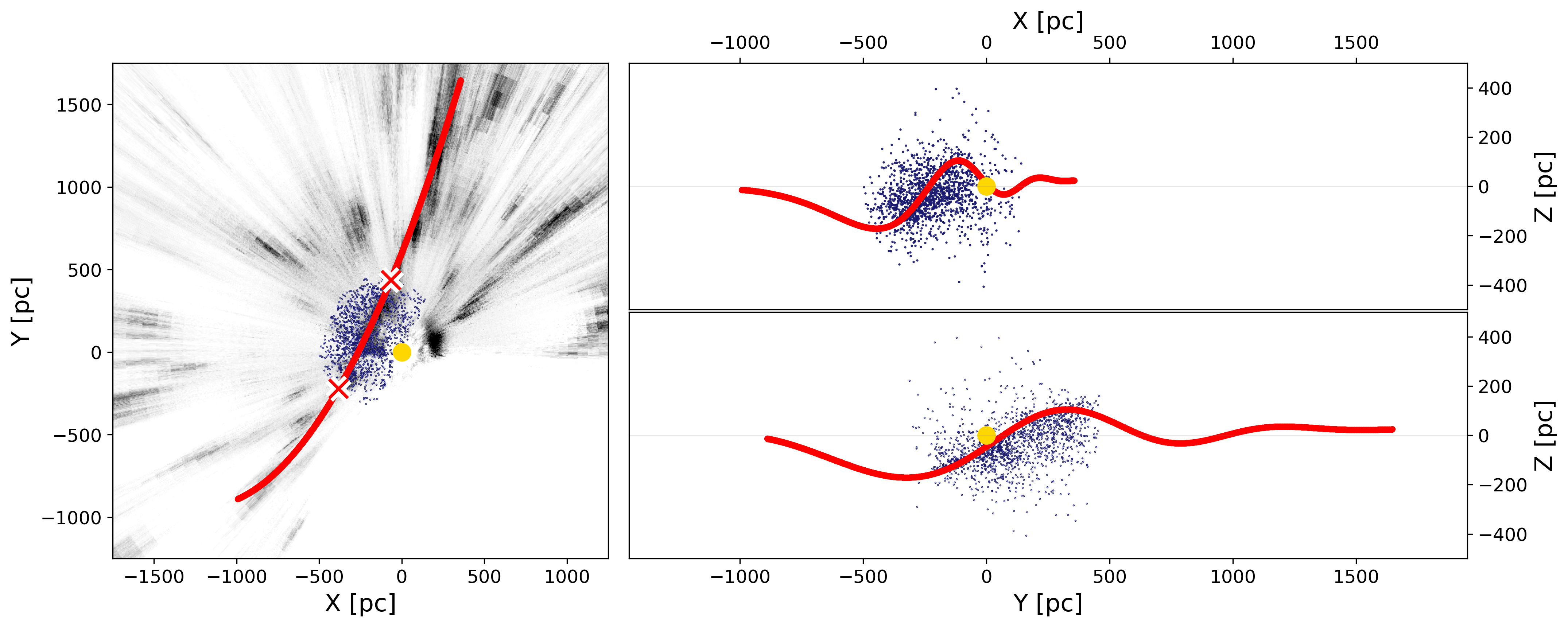
Figure 1: 3D distribution of young stars alongside the the Radcliffe Wave. We show XY (left), XZ (top right), and YZ (bottom right) projections. The navy points represent the pre-main sequence stars (Zari et al., 2018) we use for our primary analysis without any clustering applied. The red line indicates the best-fit model of the Radcliffe Wave (Alves et al., 2020) detected in 3D dust. The 3D dust map from Green et al. (2019) integrated over the range $|Z|<300$ pc is shown in the background gray-scale in the left panel. The position of the Sun is marked with a yellow dot. The two red crosses mark the beginning $(X,Y=-385,-222)$ pc and ending $(X,Y=-67,438)$ pc positions along the wave that we consider in Figure 3.

3 Methods

Our overall methodology is straightforward. First, we convert our 6D phase space measurements (positions and velocities) to associated action-angle coordinates. Then, we want to use the distribution of the vertical angles $\Omega_{z}$ across our samples to constrain possible variations in the orbital midplane that may be associated with the Radcliffe Wave. In §3.1, we describe our approach to computing action-angle coordinates. In §3.2, we provide an overview of our modelling approach.

3.1 Conversion to Action-Angle Space

Computing actions in a known potential is a numerically challenging problem, but several methods are now publicly available (see e.g. Sanders & Binney, 2016b, for a review of different methods). We use three different methods for computing stellar actions in this work. In decreasing order of both accuracy and computational expense they are:

1. direct orbit integration,

2. the Stäckel-Fudge method, and

3. the epicyclic approximation.

We will only use the direct orbit integration to explore general trends in vertical angle (and not for our subsequent model fitting) due to its large computational expense.

The first method we use is direct orbit integration, which we consider our “gold standard” method. After transforming the stars in both the young and old samples to Heliocentric Galactic Cartesian coordinates using the astropy package (Astropy Collaboration et al., 2018), we employ the gala (Price-Whelan, 2017) implementation of the algorithm in Sanders & Binney (2014) to transform the stars to action-angle coordinates. We use gala’s built-in MilkyWayPotential, which is based on the MWPotential2014 in galpy (Bovy, 2015) and includes a Hernquist (1990) bulge and nucleus, a Miyamoto-Nagai disk (Miyamoto & Nagai, 1975), and a Navarro-Frenk-White halo (Navarro et al., 1997). For each orbit, we attempt to integrate with $10,000$ time steps of $0.5\,\text{Myr}$ each ($\sim 5\,\text{Gyr}$, or $\sim 20$ orbits for a Sun-like star) using the Dormand-Prince integrator (Dormand & Prince, 1980). If this procedure fails, we try again with 400,000 timesteps of 0.05 Myr each (after which all stars converge). As a result of this procedure, each star’s 6D position and velocity are now expressed via three action coordinates ($J_{R}$, $J_{\phi}$, $J_{z}$) and three angle coordinates ($\Omega_{R}$, $\Omega_{\phi}$, $\Omega_{z}$).

Next, we use the galpy (Bovy, 2015) implementation of the Stäckel-Fudge method (Binney, 2012). This method relies on locally approximating the potential as a Stäckel potential (de Zeeuw, 1985), and is commonly used as a fast but accurate approximation, especially for disk-like orbits (e.g. Myeong et al., 2018; Trick et al., 2019; Hunt et al., 2019). For our potential we assume the standard axisymmetric and time-invariant MWPotential2014 provided in galpy.

The final method we use to compute actions and angles is through the epicyclic approximation, which makes the assumption that the dynamics in the $R$ and $z$ directions are decoupled (for an introduction, see §3.2.3 of Binney & Tremaine, 2008). Therefore, while the previous two methods computed all three actions and angles at the same time, we can compute the vertical action and angle in isolation here. Following Beane et al. (2019), the vertical motion is assumed to be that of a harmonic oscillator with:

$$z=A_{z}\sin(\nu t+\beta)+z_{0}$$ (1)

$$v_{z}\equiv\frac{{\rm d}z}{{\rm d}t}=A_{z}\nu\cos(\nu t+\beta)+v_{z_{0}}$$ (2)

Here $A_{z}$ is the amplitude of the orbit, $\nu$ is the vertical restoring frequency, $\beta$ is an arbitrary phase, and $z_{0}$ and $v_{z_{0}}$ are the location and velocity of the midplane. Then, the vertical angle can be computed as

$$\Omega_{z}\equiv\nu t+\beta=\tan^{-1}\left(\frac{z-z_{0}}{v_{z}-v_{z_{0}}}\nu\right)$$ (3)

When using the epicyclic approximation for our subsequent modeling, we allow the value of $\nu$ to be a free parameter, although we assume there is no large-scale spatial variation. We also allow the location and velocity of the midplane to vary with position along the Radcliffe Wave.

We use the latter two methods (the Stäckel-Fudge method and the epicyclic approximation) in our model fitting, described in §3.2. We emphasize that these two methods are complementary and have differing sets of advantages and disadvantages. The Stäckel-Fudge method is more accurate than the epicyclic approximation. However, in the epicyclic approximation we do not need to assume a Galactic potential by allowing the vertical restoring frequency $\nu$ (which would depend on an assumed potential) to be a free parameter in our model fitting. Therefore, we use Stäckel-Fudge and the epicyclic approximation in tandem to build confidence in the robustness of our results.

The accuracy of the epicylic approximation (and by extension the Stäckel-Fudge method) is confirmed in Appendix B through comparison with the direct orbit integration results computed from gala. The typical error is $\approx 0.2$ radians ($\approx 3\%$). Online at the Harvard Dataverse, we provide a table summarizing the young star results for the unclustered Radcliffe Wave sample and refer interested readers there for more details (doi:10.7910/DVN/58Z87S).

3.2 Fitting a Model

In order to parameterize potential oscillatory behavior in action-angle space, we need to build a sinusoidal model to describe the structure of the Radcliffe Wave sample in position and velocity space. We will then compare this model to the action-angle data for each star, computed using both the epicylic and Stäckel-Fudge approximations.

The epicyclic approximation (Binney & Tremaine, 2008), which is quite accurate for a thin disk orbit, rests on the assumption that the orbit of a given star follows simple harmonic motion independently in the $R$ and $z$ directions. Following the epicyclic approximation from §3.1, Equation 3 provides a parameterization of the phase of the orbit in the $z$ direction $\Omega_{z}$, as a function of the vertical restoring frequency $\nu$ and the location ($z_{0}$) and velocity ($v_{z_{0}}$) of the midplane. Rather than setting $z_{0}$ and $v_{z_{0}}$ to be constants, we instead assume that they may be spatially varying as a function of position $s$ along the Radcliffe Wave in XY space (see §2) according to the following functional forms:

$$z_{0}(s)=B\sin(\omega s+\gamma)+C$$ (4)

$$v_{z_{0}}(s)=D\cos(\omega s+\gamma)+E$$ (5)

where $B$ represents the amplitude of the positional function, $C$ represents the offset of the positional function, $D$ represents the amplitude of the velocity function, $E$ represents the offset of the velocity function, $\omega$ represents angular frequency, and $\gamma$ represents a phase shift. In other words, we allow for the dynamical midplane to be “wavy” rather than flat.

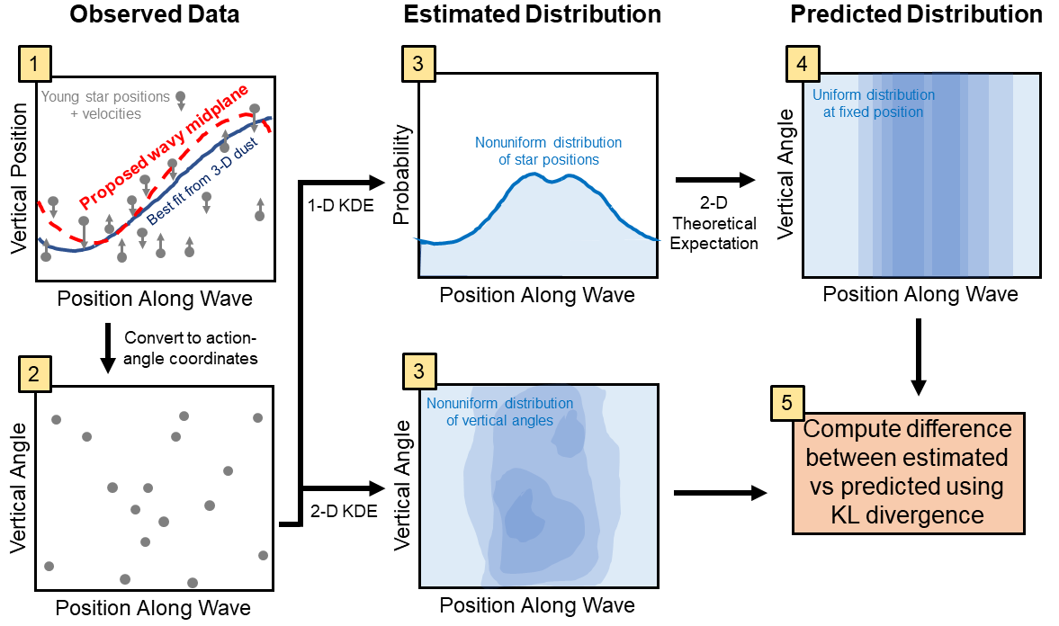
Figure 2: A schematic illustration of our modelling approach. For a proposed wavy midplane model, we take our sample of young stars (selected relative to the best-fit model of the Radcliffe Wave estimated from 3D dust) shown in the top left panel and convert their corresponding 6D positions and velocities to their corresponding action-angle coordinates. This then provides a corresponding distribution of vertical angles, as shown in the bottom left panel. Using kernel density estimation (KDE), we then estimate both the 1-D distribution in projected position along the Radcliffe Wave as well as the 2-D distribution in both projected position and vertical angle (middle panels). Based on the estimated 1-D distribution of projected positions, we then compute the expected 2-D distribution assuming all stars orbit around the proposed midplane (top right panel). We then compare the two distributions using a scaled version of the Kullblack-Leibler (KL) divergence (bottom right panel). See §3.2 for additional details.

Table 1: Priors for the Wavy Midplane Model

Parameter	Description	Prior	Units
$B$	Midplane position amplitude	${\rm Uniform}(0,300)$	pc
$\omega$	Angular frequency	${\rm Uniform}(0,4\pi)$	kpc-1
$\gamma$	Phase shift	${\rm Uniform}(0,2\pi)$	rad
$C$	Midplane position offset	${\rm Uniform}(-200,200)$	pc
$D$	Midplane velocity amplitude	${\rm Uniform}(-15,15)$	km s-1
$E$	Midplane velocity offset	${\rm Uniform}(-15,15)$	km s-1
$\nu$	Epicyclic frequency	${\rm Uniform}(0,200)$	km s-1 kpc-1

Note. — Choice of priors for the model fits described in §3.2, which we assume to be uniform over the listed ranges. Note that the epicyclic frequency $\nu$ is only modeled when using the epicyclic approximation; it is not used with the Stäckel-Fudge approximation, which assumes a known Milky Way potential.

Assuming the epicylic approximation holds, our resulting set of $\{\Omega_{z,i}(\theta)\}_{i=1}^{n}\equiv\{\Omega_{z,1}(\theta),\dots,\Omega_{z,n}(\theta)\}$ values (one for each star $i$ in our sample of $n$ stars) given the parameters $\theta\equiv(B,\omega,\gamma,C,D,E,\nu)$ that correctly describe the dynamical midplane should be uniformly distributed in angle at fixed position along the wave $s$. To determine the degree to which this behaviour holds, we therefore want to compare our observed probability distribution

$$P_{\rm obs}(\Omega_{z},s|\theta)=P_{\rm obs}(\Omega_{z}|s,\theta)\times P_{\rm obs}(s)$$ (6)

to our theoretical prediction that the conditional distribution is uniform, i.e.

$$P_{\rm unif}(\Omega_{z},s|\theta)=\frac{1}{2\pi}\times P_{\rm obs}(s)\quad\Longleftrightarrow\quad P_{\rm obs}(\Omega_{z}|s,\theta)=\frac{1}{2\pi}$$ (7)

where the conditional dependence on $\theta$ arises from the fact that changing $\theta$ affects the distribution of vertical angle ($\Omega_{z}$) but not projected position along the Radcliffe Wave ($s$).

For a given set of parameters $\theta$, we quantify the non-uniformity in the distribution by defining a (pseudo-)log-likelihood $\ln\mathcal{L}_{\rm KL}(\theta)$ based on the Kullback-Leibler (KL) divergence between $P_{\rm obs}(\Omega_{z},s|\theta)$ and $P_{\rm unif}(\Omega_{z},s|\theta)$:

$$\ln\mathcal{L}_{\rm KL}(\theta) \equiv-\xi\int P_{\rm unif}(\Omega_{z},s|\theta)\,\left[\ln P_{\rm unif}(\Omega_{z},s|\theta)-\ln P_{\rm obs}(\Omega_{z},s|\theta)\right]\,{\rm d}\Omega_{z}{\rm d}s$$ (8)

$$=\frac{\xi}{2\pi}\int P_{\rm obs}(s)\,\ln P_{\rm obs}(\Omega_{z}|s,\theta)\,{\rm d}\Omega_{z}{\rm d}s\>+\>{\rm constant}$$ (9)

where $\xi$ is a scaling constant to help ensure appropriate uncertainty estimates. We can interpret this likelihood as a weighted average over the difference in the log-probabilities between $P_{\rm unif}(\Omega_{z},s|\theta)$ (based on our hypothetical, truly uniform sample) and $P_{\rm obs}(\Omega_{z},s|\theta)$ (based on the Radcliffe Wave sample) where the weight as a function of $\Omega_{z}$ and $s$ is specified by the expected theoretical distribution $P_{\rm unif}(\Omega_{z},s)$. This quantity is maximized when the two distributions being compared are identical, i.e. when $P_{\rm unif}(\Omega_{z},s|\theta)=P_{\rm obs}(\Omega_{z},s|\theta)$or, as can be seen in the simplified version, when $P_{\rm obs}(\Omega_{z}|s,\theta)=1/2\pi$. The negative sign ensures that as the KL divergence gets smaller, our likelihood improves.

To evaluate our (pseudo-)log-likelihood function $\ln\mathcal{L}_{\rm KL}(\theta)$, we need to estimate $P_{\rm obs}(s)$ and $P_{\rm obs}(\Omega_{z},s|\theta)$ from the set of $1,000-1,500$ stars in our sample. We use a kernel density estimation (KDE) approach with a Gaussian kernel whose width is chosen to be a few percent of the overall allowed range in $s\in[0,750)$ pc and $\Omega_{z}\in[0,2\pi)$ rad to compute an estimate for $P_{\rm obs}(s)$ (once) and $P_{\rm obs}(\Omega_{z},s|\theta)$ (each time we change $\theta$). To compute an estimate of the integral, we evaluate our KDE-based estimates for a given $\theta$ over a uniformly-spaced grid spanning the same range in $s$ and $\Omega_{z}$; we find a $50\times 50$ grid is accurate enough for our purposes while remaining computationally light.

After finding the best fit value $\theta_{\rm best}$ from the data based on the unclustered young star sample, we simulate $m$ realizations of the $n$ data points using the same estimate for $P_{\rm obs}(s)$ derived previously and assuming a uniform distribution in $P(\Omega_{z}|s,\theta)$. We then compute the best-fit parameters $\{\theta_{{\rm best},j}\}_{j=1}^{m}$ for each realization. After we confirm that the best-fit solutions are unbiased relative to our simulations, we use them to determine $\xi$ so that the $1\sigma$ range in estimated values corresponds to a log-likelihood reduction of $\approx 1$, which is the expected difference assuming the distribution follows a multivariate Gaussian. We find after $m=100$ iterations that $\xi\approx 1000$ largely satisfies this constraint.

A schematic illustration of our modelling approach is shown in Figure 2.

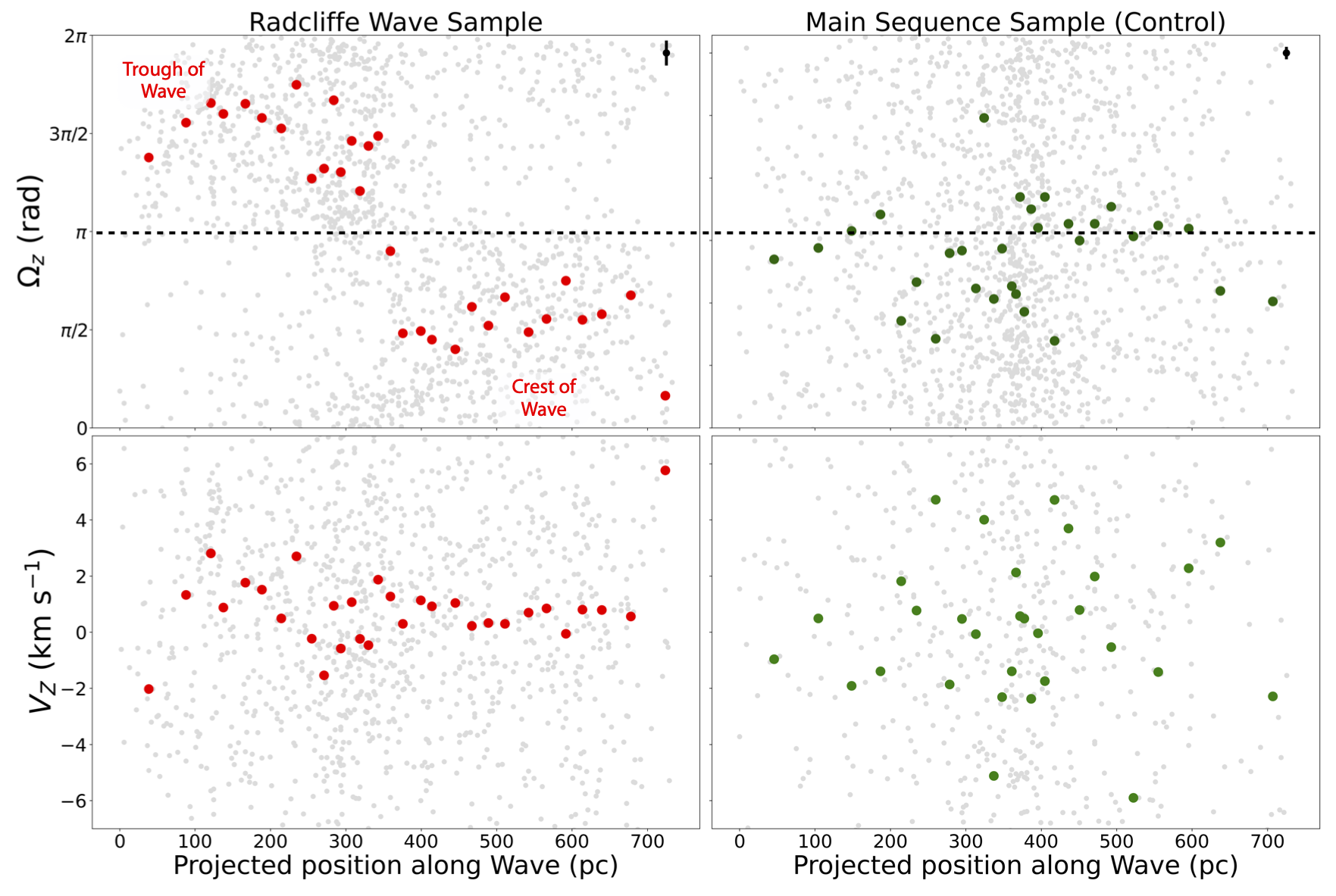
Figure 3: Top: Vertical angle vs. projected position along the Radcliffe Wave for the Radcliffe Wave pre-main sequence star sample (left) and the older Main Sequence control sample (right). The grey points represent the stars in each sample and the colored dots are the binned “phase-marginalized” medians. In the upper right hand corner of each panel we show the typical error on the vertical angle for each sample in black. In the Radcliffe Wave sample of young stars, we see a clear linear trend in phase space consistent with a wave-like oscillation. No such trend exists in the older stellar population, implying that this is not purely due to the cuts used to select both samples. Bottom: Same as the top panel, but for the vertical velocity $v_{z}$ vs. projected position along the Radcliffe Wave. Unlike with the vertical angle, we find no systematic trend in the vertical velocities of the young stars as a function of position along the wave and we detect no fluctuations in the average vertical velocity at a level $\rm\gtrapprox 3\;km\;s^{-1}$.

To estimate uncertainties on the parameters given our observed data $P(\theta|\{s_{i}\},\{\Omega_{z_{i}}\})$, we use Bayes Theorem, which can be written as:

$$P(\theta|\{s_{i}\}_{i=1}^{n},\{\Omega_{z_{i}}\}_{i=1}^{n})\propto P(\{s_{i}\}_{i=1}^{n},\{\Omega_{z_{i}}\}_{i=1}^{n}|\theta)P(\theta)\equiv\mathcal{L}_{\rm KL}(\theta)\pi(\theta)$$ (10)

where $P(\theta|\{s_{i}\}_{i=1}^{n},\{\Omega_{z_{i}}\}_{i=1}^{n})$ is the posterior distribution, $P(\{s_{i}\}_{i=1}^{n},\{\Omega_{z_{i}}\}_{i=1}^{n}|\theta)=\mathcal{L}_{\rm KL}(\theta)$ is our likelihood in Equation (8) and $P(\theta)\equiv\pi(\theta)$ is our prior. We assume flat priors on all parameters, as summarized in Table 1.

We generate samples from the posterior distribution using the nested sampling program $\tt dynesty$ (Speagle, 2020). We use the default configuration and stopping criteria, although we place a periodic boundary condition on the parameter $\gamma$. This fitting process is performed with both the clustered and unclustered Radcliffe Wave samples and with the epicyclic and Stäckel-Fudge approximations. As a control test, we also perform the fit to the older, main sequence control sample with the epicyclic approximation.

4 Results

Table 2: Parameter Estimates from the Wavy Midplane Model

Parameter	Epicyclic (Unclustered)	Epicyclic (Clustered)	Stäckel (Unclustered)	Stäckel (Clustered)
$B$	$68_{-7}^{+6}$ pc	$96_{-18}^{+15}$ pc	$65_{-9}^{+167}$ pc	$79_{-6}^{+12}$ pc
$\omega$	$6.1_{-0.9}^{+1.3}$ kpc-1	$4.6_{-0.9}^{+2.1}$ kpc-1	$5.5_{-4.4}^{+1.5}$ kpc-1	$5.3_{-1.2}^{+0.9}$ kpc-1
$\gamma$	$4.2_{-0.4}^{+0.4}$	$4.6_{-0.6}^{+0.4}$	$4.5_{-0.6}^{+1.6}$	$4.5_{-0.3}^{+0.5}$
C	$-12_{-8}^{+5}$ pc	$-2_{-10}^{+10}$ pc	$-12_{-53}^{+15}$ pc	$-11_{-6}^{+5}$ pc
D	$0.3_{-0.9}^{+0.9}$ km s-1	$1.5_{-1.6}^{+1.9}$ km s-1	$0.2_{-2.9}^{+4.1}$ km s-1	$1.6_{-1.7}^{+1.7}$ km s-1
E	$0.6_{-0.7}^{+0.7}$ km s-1	$-0.5_{-1.6}^{+1.3}$ km s-1	$0.7_{-4.2}^{+2.3}$ km s-1	$-0.4_{-1.5}^{+0.9}$ km s-1
$\nu$	$91_{-8}^{+9}$ km s-1 kpc-1	$119_{-10}^{+11}$ km s-1 kpc-1	—	—

Note. — Results of the model fitting described in §3.2 for both the clustered and unclustered Radcliffe Wave samples, fit using both the epicyclic and Stäckel-Fudge approaches. For each parameter, the median and the $2\sigma$ uncertainties (i.e. 95% credible intervals) are reported, as derived from the dynesty nested sampling results. See Table 1 for a summary of the various parameters and priors used in the analysis.

In the top panel of Figure 3, we plot the vertical angle $\Omega_{z}$ versus each star’s projected position along the wave for the primary (unclustered) young star Radcliffe Wave sample and older Main Sequence control sample, where $\Omega_{z}$ has been computed using the “gold standard” orbit integration with gala as described in §3.1 without any modifications to the orbital midplane. The individual stars in each sample are shown in light gray. The colored dots represent the median phase of the stars in each bin. Projected position is again defined as the two-dimensional distance along the wave when considering only the $x$ and $y$ coordinates. To account for periodic uncertainties in $\Omega_{z}$, we compute a “phase-marginalized” median in each bin by perturbing individual angles based on their estimated measurement uncertainty and also allowing the entire bin to experience random shifts in angle. This helps us account for possible periodic effects that may occur if the vertical angles for some stars vary around $0$ or $2\pi$ rad.

As seen in the top left panel of Figure 3, there is a noticeable trend in the vertical angle of the young star sample as we move along the Radcliffe Wave. The stars nearer to the trough of the wave generally have $\Omega_{z}\approx\frac{3\pi}{2}$, whereas the the stars nearer to the peak of the wave generally have $\Omega_{z}\approx\frac{\pi}{2}$. The trend in vertical angle is noticeably not present in the older Main Sequence sample, as seen in the top right panel of Figure 3. In the bottom panels of Figure 3, we plot vertical velocity as a function of projected position along the Radcliffe Wave for both the young star sample and the main sequence control sample. Unlike with the vertical angle, we observe no significant trend (at a level greater than $\approx$ $\rm 3.0\;km\;s^{-1}$) in the vertical velocities of young stars as a function of position along the Radcliffe Wave.

However, by convention, the vertical velocity $v_{z}$ is negative when the vertical angle is between $\frac{\pi}{2}$ and $\frac{3\pi}{2}$, while the vertical velocity is positive when the vertical angle is between $\frac{3\pi}{2}$ and $\frac{\pi}{2}$. Despite small average variations in the vertical velocity along the wave, the strong trend in vertical angle still suggests that the stars at negative $z$ (below the Galactic plane) are “on their way up” in their vertical motion (transitioning from negative $v_{z}$ to positive $v_{z}$) while the stars at positive $z$ (above the Galactic plane) are “on their way down” (transitioning from positive $v_{z}$ to negative $v_{z}$), which is fully consistent with a wave-like oscillation.

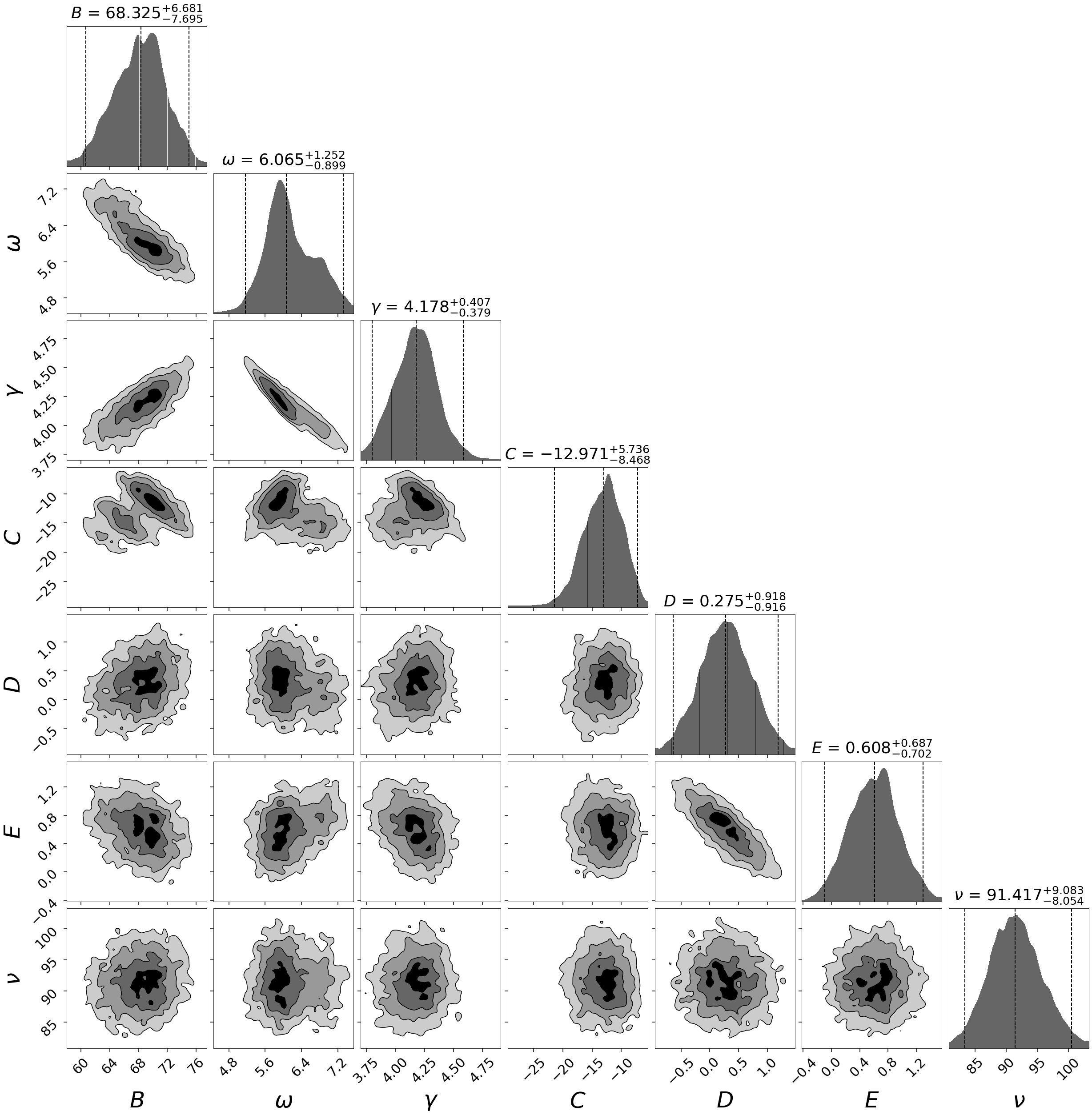
Figure 4: A cornerplot of the model parameters for the wavy midplane analysis using the epicyclic approximation and applied to the unclustered Radcliffe Wave young star sample. In the 1D distributions, the vertical dashed lines indicate the median and $2\sigma$ errors while in the 2D distributions, we demarcate the $0.5\sigma$, $1\sigma$, $1.5\sigma$, and $2\sigma$ contours. See Table 1 for a description of the parameters and associated priors.

We fit this trend in vertical angle apparent in Figure 3 using the model described in §3.2 and the $\tt dynesty$ package. A summary of our results is shown in Table 2, which includes results for both the “clustered” and “unclustered” Radcliffe Wave samples that were fit using both the epicyclic and Stäckel-Fudge approximations. We also include a corner plot for the unclustered young star sample using the epicyclic approximation, which is shown in Figure 4. Additional plots for the other three cases can be found in Appendix C. In Appendix C, we also show the results for the epicyclic fit to the main sequence control sample; the control sample fit is unconstrained, spanning a range of $3-220$ pc with most of the probability for the amplitude $B$ consistent with being $<10$ pc, in contrast to the younger sample fits.

Our best-fit amplitude for the unclustered sample based on the epicyclic approximation is $B$ = 68 pc. However, we find a significantly higher amplitude of $B$ = 96 pc when only the clustered sample is fit, implying that potential interlopers in the unclustered sample have likely been removed. We find good agreement between the epicyclic and Stäckel-Fudge best-fit parameters, with an estimated amplitude of $B$ = 65 pc and $B$ = 79 pc, respectively, for the unclustered and clustered Stäckel-Fudge samples.

We compute the best-fit period of the stellar wave using the best-fit angular frequency $\omega$ parameter, where $P=\frac{2\pi}{\omega}$. We find a best-fit period $P$ = 1.0 kpc for the epiycyclic unclustered sample (or $P$ = 1.1 kpc for the corresponding Stäckel-Fudge approach). Just like the amplitude, the period also increases when restricting the fit to the clustered stars: we obtain a period of $P$ = 1.4 kpc using the epicyclic approximation, or $P$ = 1.2 kpc when using Stäckel-Fudge approach.

Beyond the amplitude and period, we find a small value of the parameter $C$ (quantifying the offset of the midplane), which lies at $C\approx-12$ pc for three of the four fits. The $D$ parameter quantifies the deviation from the average velocity $E$ of the wave. Both of these values are also very small across all fits, on the order of $\lesssim\rm 1\;km\;s^{-1}$, implying there is not a significant velocity gradient or velocity offset of the wavy midplane.

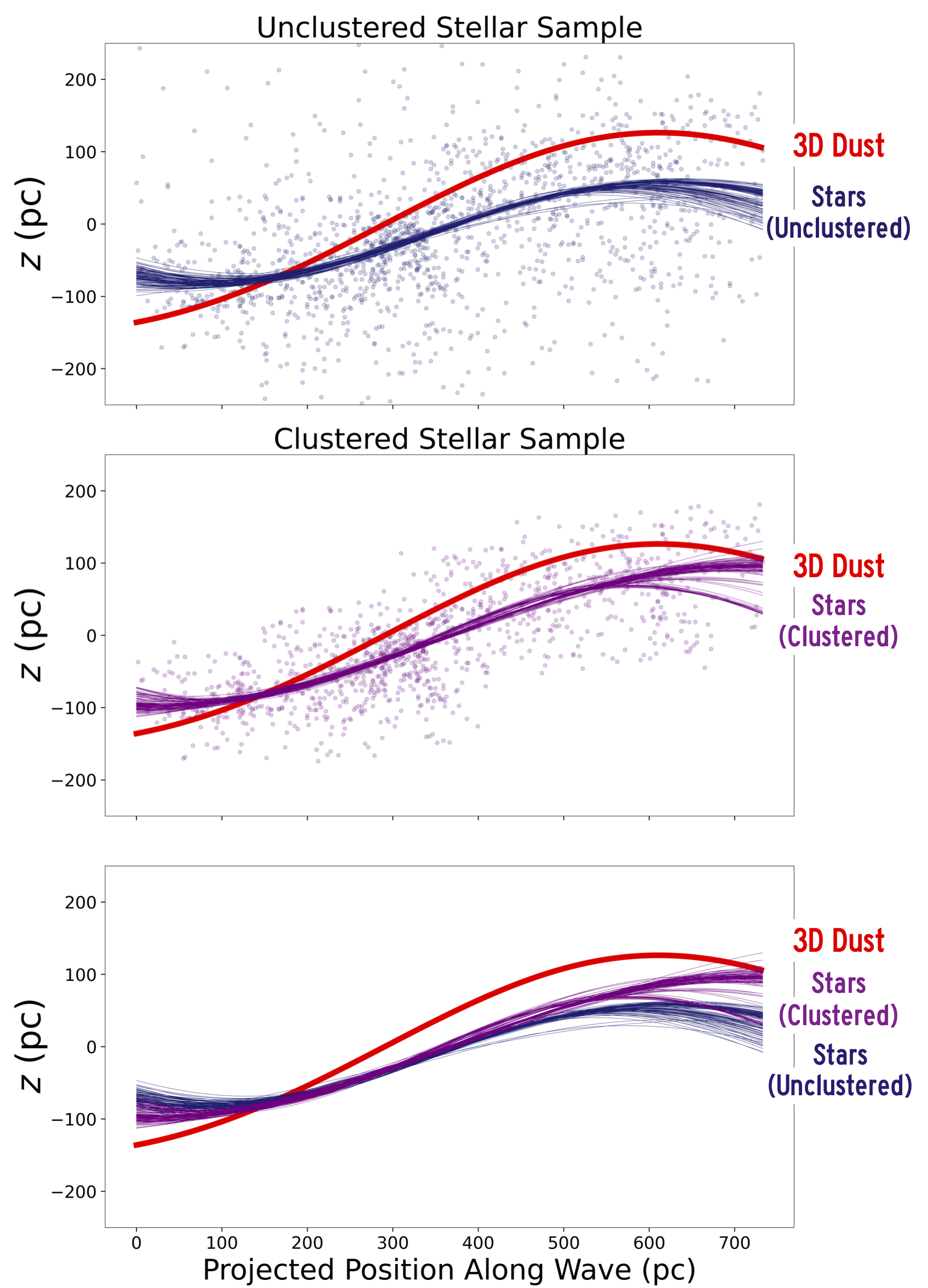
Figure 5: Comparison of the Radcliffe Wave best-fit models derived using 3D dust Alves et al. (2020) and this work. The top panel shows a comparison between the 3D dust Radcliffe Wave (red) and the epicyclic fit to the unclustered stellar wave sample (navy). The middle panel shows a comparison between the 3D dust Radcliffe Wave (red) and the epicyclic fit to the clustered stellar sample (indigo). In the bottom panel, we compare all three model fits.

5 Discussion

The ultimate goal of this work is two-fold. First, we seek to understand the differences between the Radcliffe Wave detected in 3D dust and young stars. And second, we seek to lay the foundation for understanding the Radcliffe Wave’s origin via a detailed study of its 3D kinematics.

5.1 Comparison between Stellar and Gaseous Wave

In Figure 5 we show a comparison between the best-fit model for the Radcliffe Wave defined by 3D dust, as well as our best-fit model for the Radcliffe Wave defined using the epicylic fits to the unclustered and clustered Radcliffe Wave stellar samples. For the latter, we overlay 100 realizations of the stellar sinusoidal model, based on the best-fit parameters and their corresponding errors returned by dynesty.

We find that the amplitude and period of our best-fit model to the stellar wave are smaller than, but still consistent with, the amplitude of the Radcliffe Wave detected in 3D dust. Specifically, in the 3D dust (fit to the distribution of molecular clouds), Alves et al. (2020) obtain an average amplitude and period of 160 pc and 1.9 kpc respectively when computed across the entire structure. However, computing the period and amplitude in the section of the wave overlapping with the Zari et al. (2018) sample using the dampled sinusoidal model from Alves et al. (2020), we obtain a dust-based amplitude of $B$ = 140 pc and a period $P$ = 1.5 kpc in our region of interest. Compared to the best-fit amplitude and period of $B$ = 96 pc and $P$ = 1.4 kpc derived using the clustered epicyclic results, we find overall good agreement between the stellar and interstellar Radcliffe Wave. The smaller than expected amplitude in the stellar wave could be intrinsic, in that the gas is physically leading or trailing the stars in our region of interest. However, the offset could also be due to the range of the Radcliffe Wave over which we fit: including stars only out to 500 pc in distance means our sample barely reaches the trough and crest of the wave compared to the 3D dust, which could bias our results toward lower amplitudes.

Bolstering these results, wave-like structures with similar amplitudes and periods have been detected in the dust lanes of external galaxies. For example, Matthews & Uson (2008) and Narayan et al. (2020) detect corrugations in several edge-on disk galaxies, which have amplitudes between $\approx 70-200$ pc and periods between $\approx 1-5$ kpc, consistent with both the stellar Radcliffe Wave constrained here and the gaseous Radcliffe Wave from Alves et al. (2020).

5.2 Origin of the Radcliffe Wave

The origin of the Radcliffe Wave could stem from a number of physical processes that can induce undulations in the disks of spiral galaxies. These processes can be external or internal to the disk.

Potential external causes include perturbers (dwarf galaxies, dark matter subhaloes) and/or tidal interactions with companion galaxies (e.g. López-Corredoira et al., 2002; Widrow et al., 2014). For example, past studies have discovered wave-like asymmetries in the Galactic disk by analyzing both the number density of stars and their vertical velocities at varying $z$ (Widrow et al., 2012; Bennett & Bovy, 2019), finding that a single external perturber event (occurring between 300 and 900 Myr) is responsible (Antoja et al., 2018) for the disk asymmetries in the solar neighborhood. The favored hypothesis for such a perturbation is a fly-by from a satellite. Various simulations have reproduced the Milky Way’s spiral arms and vertical oscillations with the Sagittarius dwarf galaxy (Sgr), under the constraint that the initial mass of Sgr is more massive than previously assumed (Laporte et al., 2019; Bland-Hawthorn et al., 2019). In contrast, Bennett & Bovy (2021) have argued through a suite of N-body simulations that Sgr could not have produced the vertical waves in Bennett & Bovy (2019).

Building on the work of both Bennett & Bovy (2019) and Antoja et al. (2018), Thulasidharan et al. (2021) explore the possibility that the Radcliffe Wave is indeed associated with a large-scale vertical kinematic oscillation in the disk. Based on a sample of open clusters, Upper Main Sequence (UMS) stars, OB stars, and Red Giant Branch (RGB) stars co-spatial with the Radcliffe Wave, Thulasidharan et al. (2021) find a consistent kinematic wave-like behavior in the vertical velocity (on the order of a few $\rm km\;s\;^{-1}$) in the UMS, OB, and open cluster population, but not in the older RGB population. Running N-body simulations of a satellite as massive as the Sgr dwarf galaxy impacting the galactic disk, Thulasidharan et al. (2021) conclude that the resultant density wave aligns with the Radcliffe Wave, suggesting the wave may be the result of an external perturber. However, Thulasidharan et al. (2021) also note a misalignment between this density wave and the resulting kinematic wave, which will require further follow-up work with Gaia DR3.

In comparison to Thulasidharan et al. (2021), we explore a much younger stellar population (ages of $<20$ Myr) as opposed to $\lesssim 100$ Myr in that work. We find no sinusoidal trend in vertical angle in the older main sequence population. In the case of an external perturber, it is possible that we are simply less sensitive to trends in vertical angle in the main sequence control sample, because the older stars have relaxed in comparison to the younger, dynamically colder pre-main sequence population. However, the trend in vertical angle in the youngest stellar populations $<20$ Myr most strongly associated with the gas could also favor more transitory and/or recent dynamical processes for the formation of the Radcliffe Wave. These transitory processes could include physical mechanisms internal to the disk, which, unlike a perturber, would only affect the motion of the gas, as opposed to all main sequence stars in the vicinity of the Radcliffe Wave. The pre-main sequence stars would then inherit the structure and motion of its natal material, accounting for this discrepancy in vertical angle between the younger and older stellar populations.

For example, in the spirit of Nelson & Tremaine (1995), Fleck (2020) suggests a Kelvin-Helmholtz fluid instability (KHI) arising from the cross-rotation of (i.e. difference in angular velocity between) gas in the Galactic disk and halo could give rise to a wave-like structure. Another scenario includes clustered supernova feedback, which simulations have shown are capable of pushing gas hundreds of parsecs out of the plane (Kim & Ostriker, 2018). However, the supernova-driven scenario would require a high degree of coordination along the wave’s 2.7 kpc length, rendering this mechanism somewhat less plausible than the KHI.

5.3 Velocity Variations along the Radcliffe Wave

Independent of the origin for the spatial undulation in the Radcliffe Wave, we do not detect any bulk velocity structure of the gas, as evidenced by the small values of the $D$ (quantifying the velocity offset of the midplane) and $E$ (quantifying the deviation from the average velocity) parameters in Table 2. The fact that we do not detect any additional velocity structure suggests that the velocity variation must be on the order of a few $\rm km\;s^{-1}$, which is consistent with Thulasidharan et al. (2021). The small scale of the velocity variations is also consistent with the maximum vertical velocity of stars at the midplane of $\rm\lesssim 10\;km\;s^{-1}$ predicted by the epicyclic approximation in Equation 2 ($v_{z_{max}}\approx A_{z}\times\nu$) adopting the restoring frequency $\nu$ from Table 2 and an amplitude of the stellar orbit, $A_{Z}$, equal to the amplitude of the stellar Radcliffe Wave. Any proposed origin for the Radcliffe Wave should thus not require vertical velocity variations across the wave of $\rm>10\;km\;s^{-1}$. Future observations will allow for more sensitive determinations of the velocity variation. Gaia DR3 includes a factor of four more stars with radial velocities compared to our current Gaia DR2 radial velocity sample, and these radial velocities are accompanied by smaller uncertainties. Likewise, recent work exploring the detailed structure of the Radcliffe Wave using complementary tracers, including OB stars (Pantaleoni González et al., 2021) and the youngest open clusters (Donada & Figueras, 2021), provide additional means for understanding the kinematics of the Radcliffe Wave using different stellar populations. The combination of all of the above will enable us to revisit these results in more detail, mitigating the effect of the small sample size and large radial velocity errors in our current analysis.

6 Conclusion

We leverage a sample of $\approx$ 1500 young, pre-main sequence stars (Zari et al., 2018) with radial velocity measurements from Gaia to explore the spatial and kinematic structure of the Radcliffe Wave – a 2.7 kpc band of molecular clouds recently discovered via 3D dust mapping Alves et al. (2020). Our main conclusions are as follows:

• We convert the stars’ positions and velocities to action-angle coordinates and explore trends in the stars’ vertical angle ($\Omega_{z}$) versus their position along the Radcliffe Wave. We uncover a significant trend in vertical angle indicative of a wave-like oscillation, which is not present in a control sample of older main sequence stars. The lack of a trend in vertical angle for older stars may favor a younger dynamical interpretation for the wave’s origin.

• We fit a sinusoidal model to the vertical angle data for the Radcliffe Wave’s young stars. We compare the best-fit results for the stars with the known parameters of the gaseous Radcliffe Wave detected in 3D dust: we find good morphological agreement, albeit with the stellar data favoring a smaller amplitude and period than the 3D-dust-based results.

• We do not detect significant variation in the vertical velocities as a function of position along the wave, suggesting that such variations would need to be smaller than a few kilometers per second. Future work incorporating the abundance of radial velocities in Gaia DR3 will enable more sensitive constraints on the variation in the vertical velocities and its implications for the origin of the Radcliffe Wave.

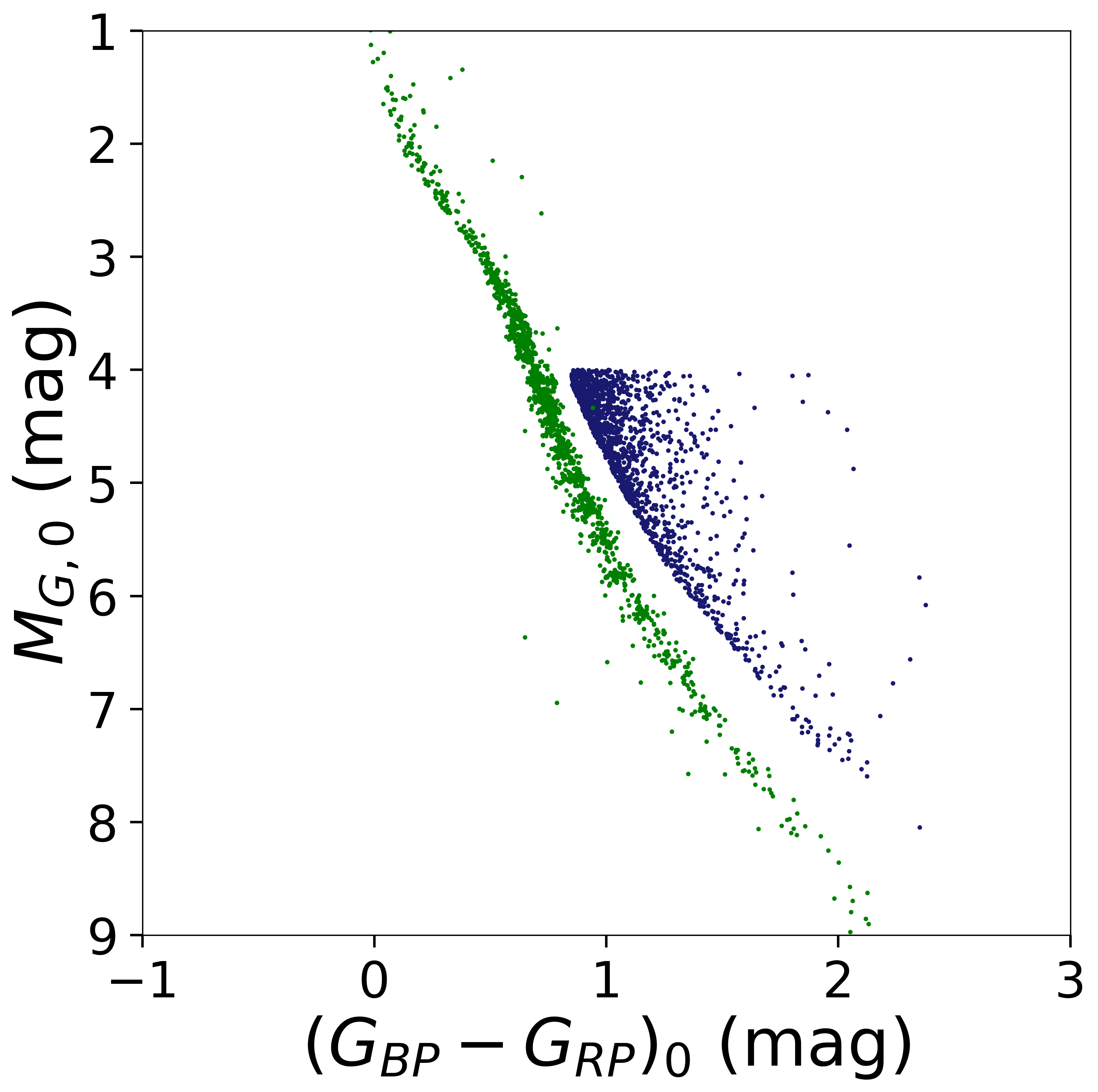
Figure 6: Dereddened Gaia-based color-magnitude diagram showing the primary unclustered pre-main sequence sample (navy) alongside the main sequence control sample (green). The sharp cutoff in $M_{G},0$ for the pre-main sequence sample is stipulated in Zari et al. (2018) and motivated by the need to exclude sources that are located on the main-sequence turn-off and on the faint end of the giant branch.

Appendix A Color-Magnitude Diagrams of Young and Old Stellar Samples

To demonstrate that our control sample truly consists of older stars, we show a dereddened Gaia-based color-magnitude diagram (CMD) in Figure 6. As expected, there is a clear differentiation between the young (PMS) stars and the older control sample, with the PMS sample showing redder $BP-RP$ colors at fixed $G$ band absolute magnitude.

Appendix B Comparisons of action-angle approximation methods: gala orbit integration vs. epicyclic approximation

The gala package uses a computationally expensive algorithm to calculate actions and angles. However, a simpler, albeit less precise, method relies on the epicyclic approximation, which we use for fitting the sinusoidal model described in §3. Here we compare the two methods to determine whether the epicyclic approximation is performing well. Setting the offsets $z_{0}$ and $v_{z_{0}}$ to zero, Equation 3 tells us that vertical angle is approximately:

$$\Omega_{z,\text{epi}}\approx\tan^{-1}\left(\frac{z}{v_{z}}\nu\right).$$ (B1)

The galpy package gives a value of $\nu\approx 75\;\rm km\;s^{-1}$ kpc^-1 as the default vertical frequency of its MWPotential2014. For each star in the Radcliffe sample, we compute the epicyclic value $\Omega_{\rm z,epi}$, then compare it to the gala-computed value $\Omega_{z,\text{gala}}$. The ratios are shown in a histogram in Figure 7. We find a that the histogram peaks around zero with a relatively small scatter ($\lesssim 0.25$) indicating that the epicyclic approach is consistent with the more expensive gala approach for our sample.

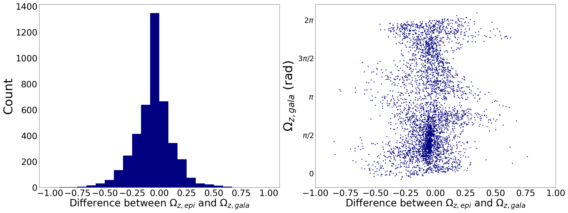
Figure 7: Left: Distribution of the difference in vertical angle value between the epicyclic approximation and direct integration of the orbit with gala for each of the stars with radial velocities in the unclustered pre-main sequence sample from Zari et al. (2018). A difference of zero denotes a perfect match. Right: The difference instead plotted against the vertical angle calculated from gala, highlighting that the greatest discrepancies occur near $0$, $\pi$, and $2\pi$.

Appendix C Additional Wavy Midplane Model Results

In the main text we summarized the overall parameter estimates derived from our four model fits to the young, pre-main sequence Radcliffe Wave sample and highlighted a summary of the results using the epicyclic approximation over the unclustered sample in Figure 4. The corner plots for the epicyclic approximation over the clustered sample, the Stäckel-Fudge approximation over the unclustered sample, and the Stäckel-Fudge approximation over the clustered sample can be found in Figures 8, 9, and Figure 10, respectively. In Figure 11, we also show the results of fitting the wavy midplane model to a sample of randomly selected, older main sequence stars occupying the same volume as the younger Radcliffe Wave sample. Unlike for the younger Radcliffe Wave sample, we find the control sample fit to be unconstrained and encompassing the most of the prior bounds. For example, $2\sigma$ error range on the amplitude $B$ spans $3-220$ pc, with most of the probability consistent with an amplitude $B<10$ pc.

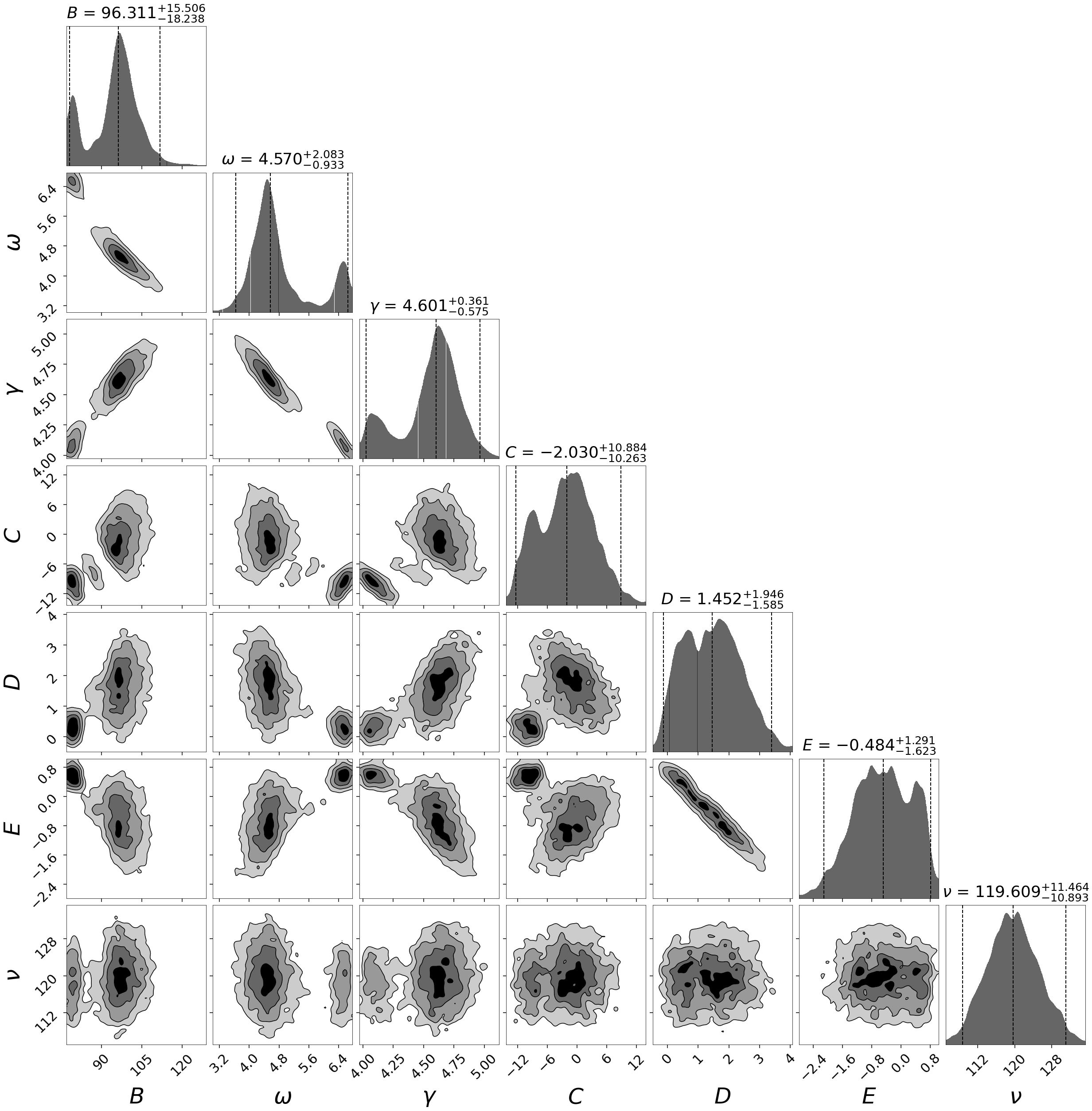
Figure 8: Same as Figure 4, but for the epicyclic approximation applied to the clustered Radcliffe Wave sample.

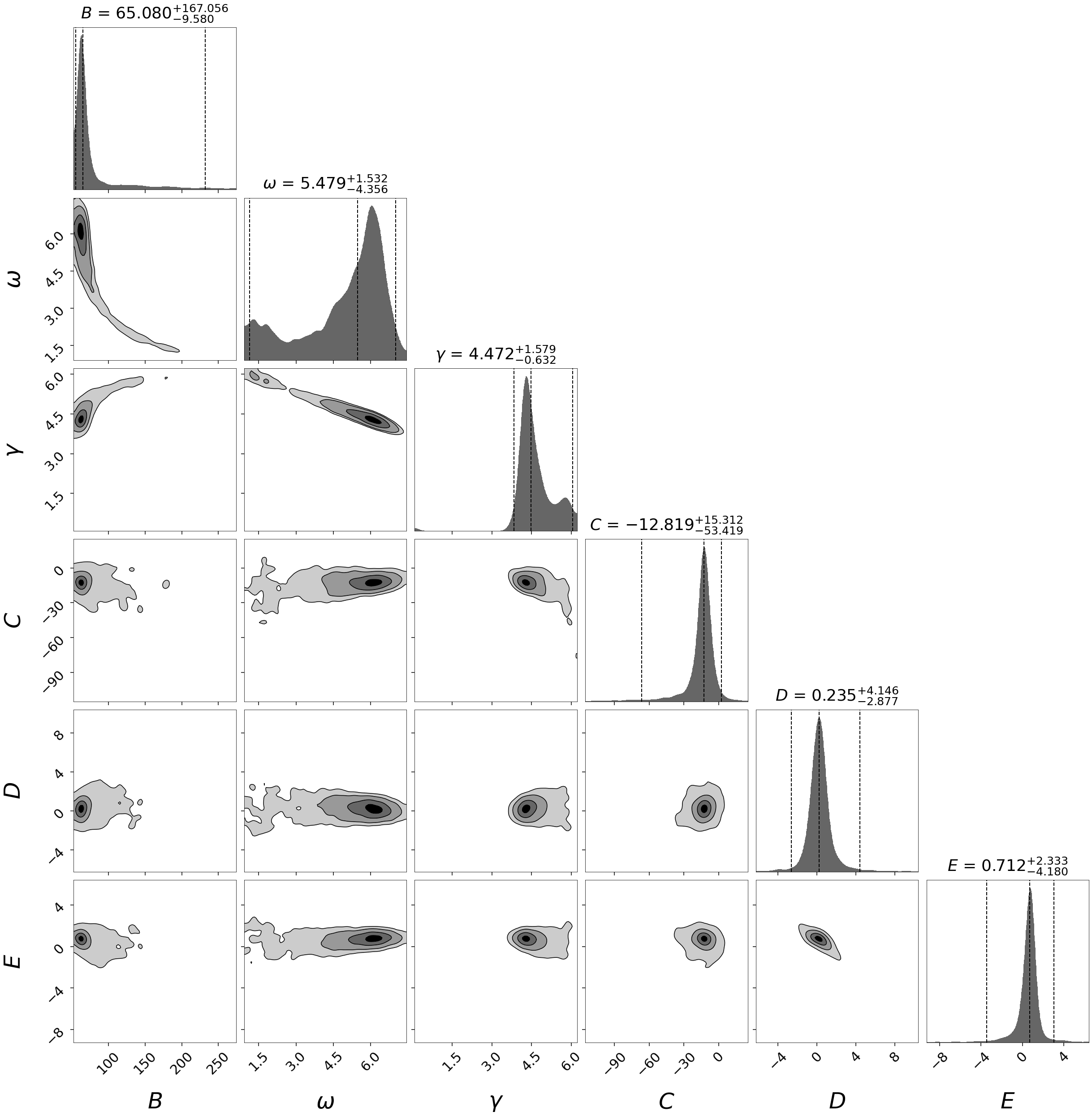
Figure 9: Same as Figure 4, but for the Stäckel-Fudge approach applied to the unclustered Radcliffe Wave sample.

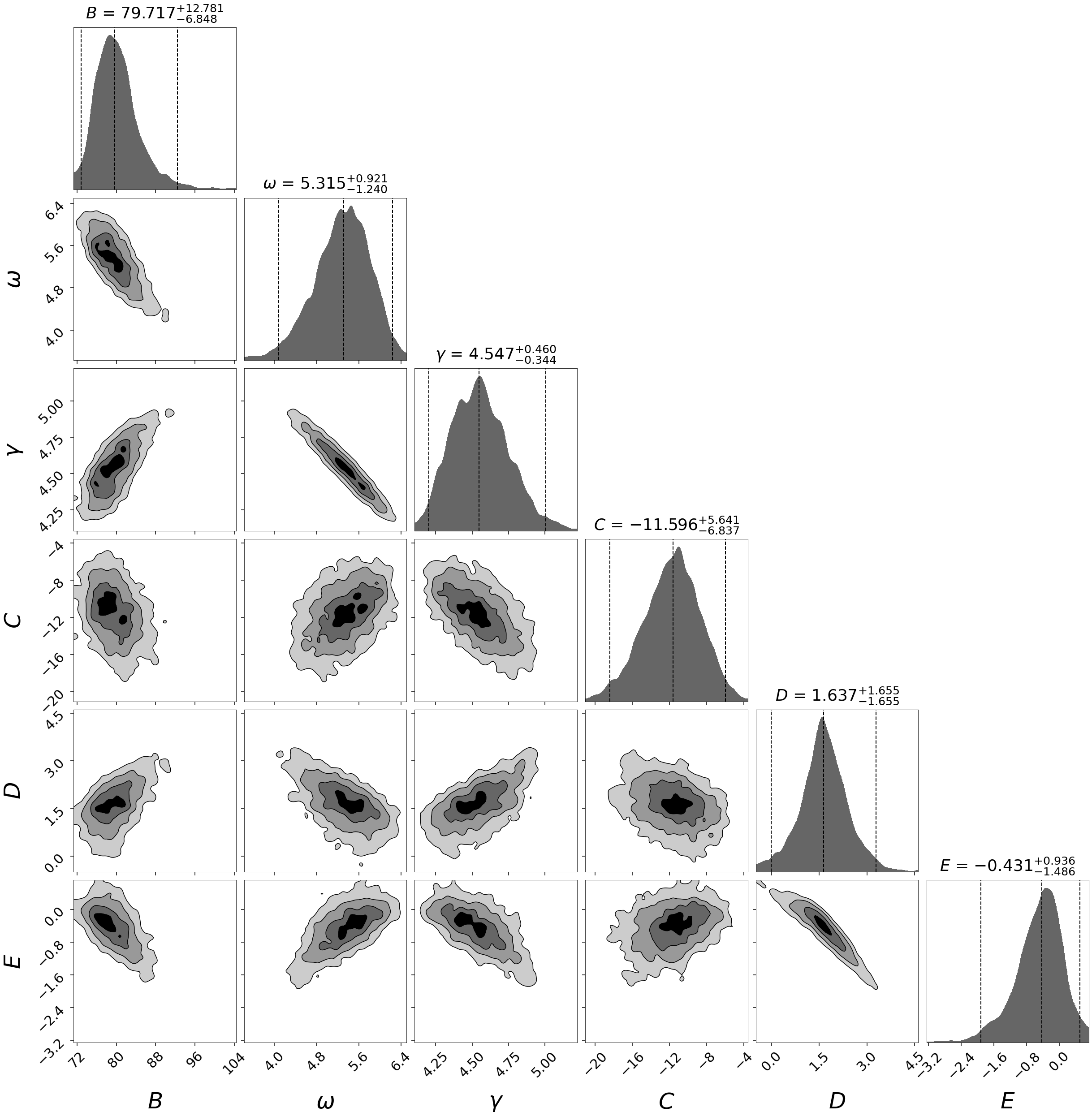
Figure 10: Same as Figure 4, but for the Stäckel-Fudge approach applied to the clustered Radcliffe Wave sample.

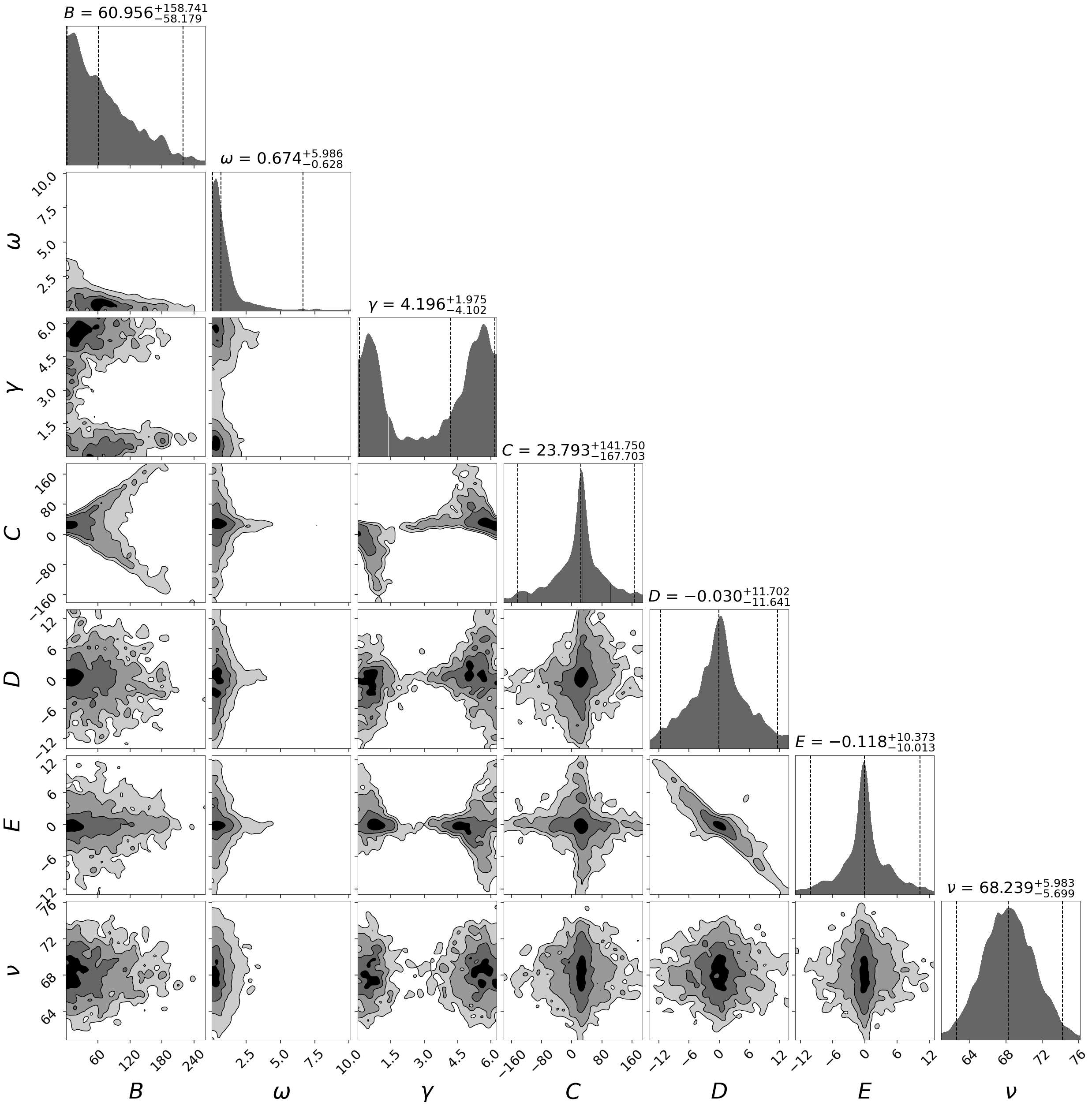
Figure 11: Same as Figure 4, but for the epicyclic approach applied to a random control sample of older, main sequence stars occupying the same volume as the younger, Radcliffe Wave sample.

References

- Alves et al. (2020) Alves, J., Zucker, C., Goodman, A. A., et al. 2020, Nature, 578, 237, doi: 10.1038/s41586-019-1874-z
- Antoja et al. (2018) Antoja, T., Helmi, A., Romero-Gómez, M., et al. 2018, Nature, 561, 360, doi: 10.1038/s41586-018-0510-7
- Astropy Collaboration et al. (2013) Astropy Collaboration, Robitaille, T. P., Tollerud, E. J., et al. 2013, A&A, 558, A33, doi: 10.1051/0004-6361/201322068
- Astropy Collaboration et al. (2018) Astropy Collaboration, Price-Whelan, A. M., Sipőcz, B. M., et al. 2018, AJ, 156, 123, doi: 10.3847/1538-3881/aabc4f
- Beane et al. (2018) Beane, A., Ness, M. K., & Bedell, M. 2018, ApJ, 867, 31, doi: 10.3847/1538-4357/aae07f
- Beane et al. (2019) Beane, A., Sanderson, R. E., Ness, M. K., et al. 2019, ApJ, 883, 103, doi: 10.3847/1538-4357/ab3d3c
- Beaumont et al. (2015) Beaumont, C., Goodman, A., & Greenfield, P. 2015, in Astronomical Society of the Pacific Conference Series, Vol. 495, Astronomical Data Analysis Software an Systems XXIV (ADASS XXIV), ed. A. R. Taylor & E. Rosolowsky, 101
- Bennett & Bovy (2019) Bennett, M., & Bovy, J. 2019, MNRAS, 482, 1417, doi: 10.1093/mnras/sty2813
- Bennett & Bovy (2021) —. 2021, MNRAS, 503, 376, doi: 10.1093/mnras/stab524
- Binney (2012) Binney, J. 2012, MNRAS, 426, 1324, doi: 10.1111/j.1365-2966.2012.21757.x
- Binney & Tremaine (2008) Binney, J., & Tremaine, S. 2008, Galactic Dynamics: Second Edition
- Bland-Hawthorn & Tepper-García (2021) Bland-Hawthorn, J., & Tepper-García, T. 2021, MNRAS, doi: 10.1093/mnras/stab704
- Bland-Hawthorn et al. (2019) Bland-Hawthorn, J., Sharma, S., Tepper-Garcia, T., et al. 2019, MNRAS, 486, 1167, doi: 10.1093/mnras/stz217
- Bovy (2015) Bovy, J. 2015, ApJS, 216, 29, doi: 10.1088/0067-0049/216/2/29
- Chen et al. (2020) Chen, B., D’Onghia, E., Alves, J., & Adamo, A. 2020, A&A, 643, A114, doi: 10.1051/0004-6361/201935955
- de Zeeuw (1985) de Zeeuw, T. 1985, MNRAS, 216, 273, doi: 10.1093/mnras/216.2.273
- Deason et al. (2017) Deason, A. J., Belokurov, V., Erkal, D., Koposov, S. E., & Mackey, D. 2017, MNRAS, 467, 2636, doi: 10.1093/mnras/stx263
- Donada & Figueras (2021) Donada, J., & Figueras, F. 2021, arXiv e-prints, arXiv:2111.04685. https://arxiv.org/abs/2111.04685
- Dormand & Prince (1980) Dormand, J., & Prince, P. 1980, Journal of Computational and Applied Mathematics, 6, 19, doi: https://doi.org/10.1016/0771-050X(80)90013-3
- Ester et al. (1996) Ester, M., Kriegel, H.-P., Sander, J., & Xu, X. 1996, in Proceedings of the Second International Conference on Knowledge Discovery and Data Mining, KDD’96 (AAAI Press), 226–231
- Fleck (2020) Fleck, R. 2020, Nature, 583, E24, doi: 10.1038/s41586-020-2476-5
- Foster et al. (2015) Foster, J. B., Cottaar, M., Covey, K. R., et al. 2015, ApJ, 799, 136, doi: 10.1088/0004-637X/799/2/136
- Gaia Collaboration et al. (2018) Gaia Collaboration, Brown, A. G. A., Vallenari, A., et al. 2018, A&A, 616, A1, doi: 10.1051/0004-6361/201833051
- Galli et al. (2019) Galli, P. A. B., Loinard, L., Bouy, H., et al. 2019, A&A, 630, A137, doi: 10.1051/0004-6361/201935928
- Green et al. (2019) Green, G. M., Schlafly, E., Zucker, C., Speagle, J. S., & Finkbeiner, D. 2019, ApJ, 887, 93, doi: 10.3847/1538-4357/ab5362
- Großschedl et al. (2021) Großschedl, J. E., Alves, J., Meingast, S., & Herbst-Kiss, G. 2021, A&A, 647, A91, doi: 10.1051/0004-6361/202038913
- Hacar et al. (2016) Hacar, A., Alves, J., Forbrich, J., et al. 2016, A&A, 589, A80, doi: 10.1051/0004-6361/201527805
- Hernquist (1990) Hernquist, L. 1990, ApJ, 356, 359, doi: 10.1086/168845
- Hunt et al. (2019) Hunt, J. A. S., Bub, M. W., Bovy, J., et al. 2019, MNRAS, 490, 1026, doi: 10.1093/mnras/stz2667
- Hunter (2007) Hunter, J. D. 2007, Computing in Science & Engineering, 9, 90, doi: 10.1109/MCSE.2007.55
- Kim & Ostriker (2018) Kim, C.-G., & Ostriker, E. C. 2018, ApJ, 853, 173, doi: 10.3847/1538-4357/aaa5ff
- Lada & Lada (2003) Lada, C. J., & Lada, E. A. 2003, ARA&A, 41, 57, doi: 10.1146/annurev.astro.41.011802.094844
- Laporte et al. (2019) Laporte, C. F. P., Minchev, I., Johnston, K. V., & Gómez, F. A. 2019, MNRAS, 485, 3134, doi: 10.1093/mnras/stz583
- López-Corredoira et al. (2002) López-Corredoira, M., Betancort-Rijo, J., & Beckman, J. E. 2002, A&A, 386, 169, doi: 10.1051/0004-6361:20020229
- Matthews & Uson (2008) Matthews, L. D., & Uson, J. M. 2008, ApJ, 688, 237, doi: 10.1086/592086
- Miyamoto & Nagai (1975) Miyamoto, M., & Nagai, R. 1975, PASJ, 27, 533
- Myeong et al. (2018) Myeong, G. C., Evans, N. W., Belokurov, V., Sanders, J. L., & Koposov, S. E. 2018, ApJ, 856, L26, doi: 10.3847/2041-8213/aab613
- Narayan et al. (2020) Narayan, C. A., Dettmar, R.-J., & Saha, K. 2020, MNRAS, 495, 3705, doi: 10.1093/mnras/staa1400
- Navarro et al. (1997) Navarro, J. F., Frenk, C. S., & White, S. D. M. 1997, ApJ, 490, 493, doi: 10.1086/304888
- Nelson & Tremaine (1995) Nelson, R. W., & Tremaine, S. 1995, MNRAS, 275, 897, doi: 10.1093/mnras/275.4.897
- Ness et al. (2019) Ness, M. K., Johnston, K. V., Blancato, K., et al. 2019, ApJ, 883, 177, doi: 10.3847/1538-4357/ab3e3c
- Pantaleoni González et al. (2021) Pantaleoni González, M., Maíz Apellániz, J., Barbá, R. H., & Reed, B. C. 2021, MNRAS, 504, 2968, doi: 10.1093/mnras/stab688
- Pedregosa et al. (2011) Pedregosa, F., Varoquaux, G., Gramfort, A., et al. 2011, Journal of Machine Learning Research, 12, 2825
- Price-Whelan (2018) Price-Whelan, A. 2018, doi: 10.5281/zenodo.1228136
- Price-Whelan (2017) Price-Whelan, A. M. 2017, Journal of Open Source Software, 2, 388, doi: 10.21105/joss.00388
- Reid et al. (2019) Reid, M. J., Menten, K. M., Brunthaler, A., et al. 2019, ApJ, 885, 131, doi: 10.3847/1538-4357/ab4a11
- Sanders & Binney (2014) Sanders, J. L., & Binney, J. 2014, MNRAS, 441, 3284, doi: 10.1093/mnras/stu796
- Sanders & Binney (2016a) —. 2016a, MNRAS, 457, 2107, doi: 10.1093/mnras/stw106
- Sanders & Binney (2016b) —. 2016b, MNRAS, 457, 2107, doi: 10.1093/mnras/stw106
- Speagle (2020) Speagle, J. S. 2020, MNRAS, 493, 3132, doi: 10.1093/mnras/staa278
- Thulasidharan et al. (2021) Thulasidharan, L., D’Onghia, E., Poggio, E., et al. 2021, arXiv e-prints, arXiv:2112.08390. https://arxiv.org/abs/2112.08390
- Trick et al. (2019) Trick, W. H., Coronado, J., & Rix, H.-W. 2019, MNRAS, 484, 3291, doi: 10.1093/mnras/stz209
- Trick et al. (2021) Trick, W. H., Fragkoudi, F., Hunt, J. A. S., Mackereth, J. T., & White, S. D. M. 2021, MNRAS, 500, 2645, doi: 10.1093/mnras/staa3317
- Widrow et al. (2014) Widrow, L. M., Barber, J., Chequers, M. H., & Cheng, E. 2014, Monthly Notices of the Royal Astronomical Society, 440, 1971, doi: 10.1093/mnras/stu396
- Widrow et al. (2012) Widrow, L. M., Gardner, S., Yanny, B., Dodelson, S., & Chen, H.-Y. 2012, ApJ, 750, L41, doi: 10.1088/2041-8205/750/2/L41
- Zari et al. (2018) Zari, E., Hashemi, H., Brown, A. G. A., Jardine, K., & de Zeeuw, P. T. 2018, A&A, 620, A172, doi: 10.1051/0004-6361/201834150
- Zucker et al. (2020) Zucker, C., Speagle, J. S., Schlafly, E. F., et al. 2020, A&A, 633, A51, doi: 10.1051/0004-6361/201936145
- Zucker & Speagle et al. (2019) Zucker & Speagle, C. . J. S., Schlafly, E. F., Green, G. M., et al. 2019, ApJ, 879, 125, doi: 10.3847/1538-4357/ab2388