Skyrme-Hartree-Fock-Bogoliubov mass models on a 3D mesh: II. time-reversal symmetry breaking.

Abstract

Models based on nuclear energy density functionals can provide access to a multitude of observables for thousands of nuclei in a single framework with microscopic foundations. Such models can rival the accuracy of more phenomenological approaches, but doing so requires adjusting parameters to thousands of nuclear masses. To keep such large-scale fits feasible, several symmetry restrictions are generally imposed on the nuclear configurations. One such example is time-reversal invariance, which is generally enforced via the Equal Filling Approximation (EFA). Here we lift this assumption, enabling us to access the spin and current densities in the ground states of odd-mass and odd-odd nuclei and which contribute to the total energy of such nuclei through so-called ‘time-odd’ terms. We present here the Skyrme-based BSkG2 model whose parameters were adjusted to essentially all known nuclear masses without relying on the EFA, refining our earlier work [G. Scamps et al., EPJA 57, 333 (2021)]. Moving beyond ground state properties, we also incorporated information on the fission barriers of actinide nuclei in the parameter adjustment. The resulting model achieves a root-mean-square (rms) deviation of (i) 0.678 MeV on 2457 known masses, (ii) 0.027 fm on 884 measured charge radii, (iii) 0.44 MeV and 0.47 MeV, respectively, on 45 reference values for primary and secondary fission barriers of actinide nuclei, and (iv) 0.49 MeV on 28 fission isomer excitation energies. We limit ourselves here to a description of the model and the study the impact of lifting the EFA on ground state properties such as binding energies, deformation and pairing, deferring a detailed discussion of fission to a forthcoming paper.

1 Introduction

Nucleosynthesis simulations, and in particular those dealing with the r-process, require nuclear data across the nuclear chart for several different quantities Arnould20 . For the overwhelming majority of nuclei, experimental information on observables such as the binding energy is unavailable due to the difficulty of synthesising and detecting short-lived neutron-rich nuclei in accelerators and laboratories. Even for nuclei close to stability, more complex quantities such as nuclear level densities and the $\gamma$-ray strength function can be either difficult or just very expensive to measure.

Nuclear theory needs to fill this knowledge gap by constructing models capable of providing reliable extrapolations for nuclei at the extremes of energy, angular momentum and isospin. The complexity of the nuclear many-body problem implies that such systematic modelling of multiple thousands of (mostly heavy) nuclei cannot be tackled from first principles, despite the recent successes of ab initio approaches Hergert20 . Some degree of phenomenology in a global nuclear model is thus unavoidable, but too much of it negatively impacts the reliability of extrapolations to exotic nuclei.

Methods based on energy density functionals (EDFs) provide an attractive compromise: they provide access to many different quantities of interest in a consistent framework with microscopic foundations, while calculations for thousands of nuclei remain feasible Bender03 ; Goriely16 . A nuclear EDF links the energy of a nucleus to the precise configuration of its nucleonic densities through coupling constants, which are the main source of phenomenology in these approaches. Theory offers little a priori information on the values of these (often numerous) constants, such that they need to be fitted to experimental data. Many different fitting strategies for several different types of EDFs have been suggested in the literature Dutra12 ; Dutra14 , aimed at producing models with differing goals and regions of applicability.

If furnishing data to applications is the goal, it is natural to impose an excellent global reproduction of nuclear masses, as these set the energy scales involved in nuclear reactions and decays. The Brussels-Montréal (BSk) models, based on EDFs of the Skyrme type, have shown that incorporating essentially all known masses in the fit protocol leads to an excellent description of masses. The members of the BSk-family achieve a root-mean-square (rms) deviation typically below 800 keV, and often close to 500 keV Goriely16 ; Goriely13a , which is competitive with the global nuclear models that have less microscopic foundations Moller16 . Furthermore, this accuracy for the masses is combined with (i) a global description of other properties of finite nuclei such as charge radii and fission barriers, and (ii) a description of infinite nuclear matter that is generally comparable to ab-initio calculations.

While central to the success of the strategy, the inclusion of thousands of masses renders the fit computationally demanding. Out of necessity, nuclei are thus typically not treated in the most general way possible during the parameter adjustment. For the BSk-family, the computational demands resulted in two practical restrictions: the nuclear configurations were (i) highly restricted by symmetry assumptions and (ii) numerically represented through an expansion of the single-particle wavefunctions in a limited number of harmonic oscillator states. These two restrictions greatly lower the computational complexity of a fit, but the first restriction limits the generality of the resulting model while the second limits its numerical accuracy.

To provide nuclear data free of these limitations, we developed in Ref. Scamps21 the first Brussels-Skyrme-on-a-Grid model, BSkG1. This model was adjusted using the MOCCa code Ryssens16 , which relies on a numerical representation of the nucleus in three-dimensional coordinate space. Such a representation allows for an improved control of numerical accuracy Ryssens15b , while imposing less stringent symmetry conditions. Where the BSk models considered all nuclei to be axially symmetric, the BSkG1 model offers a more general description of nuclear ground states by allowing for triaxial deformation. It retains the overall quality of the older models in terms of the global description of masses, charge radii and infinite nuclear matter properties. BSkG1 was but a first step in this direction, as its parameter adjustment was still limited in a number of ways Scamps21 . First, the nuclear configurations allowed for were not the most general possible, but restricted by the assumption of time-reversal invariance and reflection symmetry. Secondly, we restricted our study to nuclear ground states, ignoring the quality of the model with respect to other properties of atomic nuclei that impact astrophysical applications.

Allowing for reflection-asymmetric shapes is not a priority for a description of masses, as in a mean-field approach octupole correlations are known to impact nuclear ground states for only a very limited number of nuclei in a few isolated regions of the nuclear chart Robledo11 ; Chen21 . The situation is very different for odd-mass and odd-odd nuclei which constitute roughly three quarters of the chart of nuclei and whose ground states all have finite angular momentum, and hence break time-reversal symmetry. An internally consistent EDF-based description of such nuclei requires a many-body state that has non-vanishing time-odd spin and current densities. Through the so-called time-odd terms of the EDF Duguet2001a ; Hellemans12 , these densities also contribute to the binding energy of the nucleus.

In fact, self-consistent mean-field calculations of the ground states of even-even nuclei are among the very few exceptional cases for which breaking of time-reversal symmetry and the consideration of time-odd terms in the EDF is not necessary. For instance, time-odd terms appear naturally in methods to describe nuclear dynamics, such as time-dependent mean-field Maruhn06 and RPA approaches Bender02 ; Kortelainen15 . They also contribute in beyond-mean-field approaches like the restoration of spatial symmetries and the mixing of states with different shapes in the Generator Coordinate Method (GCM) Bonche90 or Adiabatic time-dependent HFB Hinohara06a ; Kluepfel08a ; Petrik18 ; Washiyama21a , although in most other published work on the latter the time-odd terms are usually neglected. The vast majority of excited states of all nuclei, including even-even ones, exhibit non-zero angular momentum and are affected as well, independently of the nature of the excitation: the description of rotational states through self-consistent cranking calculations introduces an external field that breaks time-reversal symmetry Bonche87 ; Dobaczewski95 , while the modelling of non-collective states breaks time-reversal through the creation of one or more quasiparticle excitations Robledo14 . Degrees of freedom that break time-reversal invariance affect other observables beyond masses, such as magnetic moments Sassarini21 .

The relevance of the time-odd terms is also not limited to finite nuclei: the time-odd spin-spin interaction terms contribute to the equation of state of spin- and spin-isospin polarised infinite homogeneous nuclear matter. Their contribution can be expected to influence the composition of neutron star crusts in the presence of strong magnetic fields Pena11 , and even induce a phase transition to homogeneous polarised matter Margueron02 ; Chamel09 ; Chamel10b ; Cao10 . Similarly, gradients of spin densities in the EDF can induce finite-size instabilities that lead to a phase transition to inhomogeneous infinite polarised matter Hellemans12 ; Pastore13 ; Pastore15 . The absence of indications of such phase transitions in finite nuclei and stellar objects however limits the range of possible coupling constants for the spin terms in the EDF.

Despite their relevance to the properties of finite nuclei and infinite matter, systematic studies of the time-odd channel of EDFs are scarce. Truly global approaches that study its impact in finite nuclei up to the drip lines are to the best of our knowledge non-existent. Most large-scale calculations employ the equal filling approximation (EFA) instead, which, eliminates all contributions of the time-odd terms by construction Perez08 . This approximation is popular for two reasons: (i) the absence of consensus in the literature on the optimal treatment of the time-odd terms, at least for EDFs of the Skyrme type and (ii) the complexity of solving the EDF equations for odd-mass and odd-odd nuclei. The technical complexity is related to practical considerations about CPU time and memory, but also due to the difficulty of reliably converging such calculations Schunck10 .

We present here the next entry in the BSkG-series, BSkG2, which moves beyond the limitations of its predecessor in two ways. First, we allow for more general nuclear configurations by lifting the assumption of time-reversal invariance, allowing for finite angular momentum in the nuclear ground state and exploring for the first time the influence of time-odd terms on the properties of finite nuclei in the context of a global EDF-based model. The resulting model offers a description of odd-mass and odd-odd nuclei that is on par with that of even-even nuclei, i.e. without invoking the EFA.

Secondly, we incorporate information on the fission barriers of actinides in the parameter readjustment in order to control the properties of the model at large deformation. Indeed, fitting a model to nuclear masses does not explore all regions of deformation space, such that a good mass fit will not necessarily guarantee accurate fission barriers. As in Ref. Goriely07 , we show it is possible to obtain drastically improved fission barriers while retaining the quality of the mass fit, through the adjustment of a phenomenological vibrational term that we did not include in the earlier BSkG1 fit. Our calculation of fission barriers, performed to adjust this vibrational term, included octupole and triaxial degrees of freedom for systems with both even and off numbers of nucleons. Due to this complexity, we postpone discussion of all our material related to fission to a forthcoming paper Ryssens22 . Here, we limit our discussion to the construction of the BSkG2 model and its description of both the ground state of finite nuclei and infinite nuclear matter.

This paper is organized as follows: we start by explaining the ingredients of the mass-model as well as the technical aspects of the calculations and parameter adjustment in Sec. 2. In Sec. 3, we discuss the models ground state and infinite nuclear matter properties. Our conclusions and outlook are presented in Sec. 4.

2 Construction of the mass model

2.1 The nuclear mass

To describe an atomic nucleus, we employ an auxiliary state of the Bogoliubov type: $|\Phi\rangle$. As for the earlier BSkG1 model Scamps21 , we define the total energy $E_{\rm tot}$ of this state:

$$E_{\rm tot} =E_{\rm HFB}+E_{\rm corr}\,.$$ (1)

The total energy consists of two parts: $E_{\rm HFB}$ is the self-consistent mean-field energy, while $E_{\rm corr}$ is a set of perturbative corrections. The total energy $E_{\rm tot}$ models minus the nuclear binding energy, $B_{\text{nuc}}(Z,N)=-E_{\rm tot}$, of a nucleus with mass number $A$, composed out of $Z$ protons and $N$ neutrons. Mass tables, however, list atomic masses, which include $Z$ bound electrons. In units of MeV, these are given by

$$M(N,Z)=E_{\rm tot}+NM_{n}+Z(M_{p}+M_{e})-B_{\rm el.}(Z)\,,$$ (2)

where $M_{n}$ and $M_{p}$ are the masses of bare nucleons, $M_{e}$ is the mass of an electron and $B_{\rm el.}(Z)$ is a simple analytical estimate for the binding energy of the electrons Lunney03 ; Wan21 . The mass excess can then be obtained by subtracting $A$ times the atomic mass unit from Eq. (2).

The mean-field energy is constructed from five contributions

$$E_{\rm HFB} =E_{\rm kin}+E_{\rm Sk}+E_{\rm pair}+E_{\rm Coul}+E^{(1)}_{\rm cm}\,,$$ (3)

which are, respectively, the contributions of the kinetic energy, the Skyrme effective interaction, a zero-range pairing interaction with appropriate cutoffs Krieger90 , the Coulomb force Goriely08 , and the one-body part of the centre-of-mass correction Bender00 . The correction energy $E_{\rm corr}$ consists of four parts:

$$E_{\rm corr} =E_{\rm rot}+E_{\rm vib}+E^{(2)}_{\rm cm}+E_{\rm W}\,,$$ (4)

which are, respectively, the rotational correction Tondeur00 , the vibrational correction Goriely13b , the two-body part of the centre-of-mass correction Bender00 , and the Wigner energy Goriely03 .

Most ingredients of the total energy are identical to those we employed in the BSkG1 model; the only exceptions are (i) the time-odd contributions to the Skyrme energy $E_{\rm Sk}$ and pairing energy $E_{\rm pair}$ and (ii) the inclusion of the vibrational correction. We will discuss these in detail below; for our treatment of all other terms, we refer the reader to Ref. Scamps21 .

2.1.1 Time-odd densities and terms

We write the Skyrme energy as an integral over an energy density, composed out of four parts $\mathcal{E}_{t,\rm e/o}$:

$$E_{\rm Sk} =\int d^{3}\mathbb{r}\sum_{t=0,1}\left[\mathcal{E}_{t,\rm e}(\mathbb{r})+\mathcal{E}_{t,\rm o}(\mathbb{r})\right]\,,$$ (5)

where $t=0,1$ is an isospin index. All contributions to the Skyrme energy are constructed from a set of five local one-body densities that characterize the auxiliary state $|\Phi\rangle$. Three of these already figured in Ref. Scamps21 : $\rho_{t}(\mathbb{r}),\tau_{t}(\mathbb{r})$ and $\mathbb{J}_{t}(\mathbb{r})$. We employ two additional densities, $\mathbb{s}_{t}(\mathbb{r})$ and $\mathbb{j}_{t}(\mathbb{r})$, which are the spin and current density respectively. Their definition in terms of the single-particle wavefunctions are standard in the literature and can be found for instance in Ref. Ryssens19 .

All five densities transform in a straightforward way under time-reversal. Using a superscript $T$ to indicate a density characterizing the time-reversed auxiliary state $\check{T}|\Phi\rangle$, we have

$$\rho_{t}^{T}(\mathbb{r}) =+\rho_{t}(\mathbb{r})\,,$$ (6a)

$$\tau_{t}^{T}(\mathbb{r}) =+\tau_{t}(\mathbb{r})\,,$$ (6b)

$$\mathbb{J}_{t}^{T}(\mathbb{r}) =+\mathbb{J}_{t}(\mathbb{r})\,,$$ (6c)

$$\mathbb{s}_{t}^{T}(\mathbb{r}) =-\mathbb{s}_{t}(\mathbb{r})\,,$$ (6d)

$$\mathbb{j}_{t}^{T}(\mathbb{r}) =-\mathbb{j}_{t}(\mathbb{r})\,.$$ (6e)

The three densities $\rho_{t}(\mathbb{r}),\tau_{t}(\mathbb{r})$ and $\mathbb{J}(\mathbb{r})$ are time-even, while $\mathbb{s}_{t}(\mathbb{r})$ and $\mathbb{j}(\mathbb{r})$ are time-odd. If we assume time-reversal invariance, meaning that the time-reversed auxiliary state is equal to the auxiliary state up to a phase, then Eqs. (6d) and (6e) imply that the spin and current density vanish identically.

The Skyrme energy densities $\mathcal{E}_{t,\rm e}(\mathbb{r})$ and $\mathcal{E}_{t,\rm o}(\mathbb{r})$ of Eq. (5) are built from suitable bilinear combinations of either time-even or time-odd local densities. The energy densities themselves are necessarily even under time-reversal, but we will follow common practice in the literature and refer to them as time-even and time-odd energy densities, respectively.

The time-even energy densities are given by

$$\mathcal{E}_{t,\rm e}(\mathbb{r}) =C^{\rho\rho}_{t}\,\rho_{t}^{2}(\mathbb{r})+C^{\rho\rho\rho^{\gamma}}_{t}\rho_{0}^{\gamma}(\mathbb{r})\,\rho_{t}^{2}(\mathbb{r})$$

$$+C^{\rho\tau}_{t}\,\rho_{t}(\mathbb{r})\,\tau_{t}(\mathbb{r})+C^{\rho\Delta\rho}_{t}\,\rho_{t}(\mathbb{r})\,\Delta\rho_{t}(\mathbb{r})$$

$$+C^{\rho\nabla\cdot J}_{t}\rho_{t}(\mathbb{r})\,\boldsymbol{\nabla}\cdot\mathbb{J}_{t}(\mathbb{r})\,,$$ (7)

which are identical to the ones of Ref. Scamps21 . The set of ten time-even coupling constants $\{C_{t}\}$ consists of combinations of ten model parameters: $t_{0-3},x_{0-3},W_{0}$ and $W_{0}^{\prime}$ Scamps21 .

The expression of Eq. (2.1.1) is very similar, but not identical, to the energy density that can be obtained as expectation value of a density-dependent two-body Skyrme interaction. The differences between the EDF used by us and such an interaction-generated functional are (i) the absence of any term bilinear in the spin-current density $J_{t,\mu\nu}(\mathbb{r})$, and (ii) the inclusion of a generalized spin-orbit term involving a second spin-orbit parameter $W_{0}^{\prime}$ as in the Skyrme models of Refs. Sharma95 ; Reinhard95 . For the reasons recalled in Ref. Lesinski07 , the former is common practice for many widely-used parameterizations of the Skyrme EDF, while the latter has become popular in recent parameter fits as it allows for better fine-tuning of spin-orbit effects by relaxing the relation $W_{0}=W_{0}^{\prime}$ of the standard spin-orbit interaction and thereby leads to linearly independent coefficients $C^{\rho\nabla\cdot J}_{0}$ and $C^{\rho\nabla\cdot J}_{1}\neq 3\,C^{\rho\nabla\cdot J}_{0}$ of the EDF. The time-even energy density of Eq. (2.1.1) is similar to the one of Refs. Klupfel09 ; Kortelainen10 ; Kortelainen14 and consists of a subset of the terms employed by later BSk models Goriely16 ; Goriely15 , omitting, however, the density-dependence of the $\rho_{t}(\mathbb{r})\tau_{t}(\mathbb{r})$ and $\rho_{t}(\mathbb{r})\Delta\rho_{t}(\mathbb{r})$ terms introduced in Ref. Chamel09 . A parameter fit of the more complete EDF of Goriely16 ; Goriely15 with the tools described here will be the subject of future work.

There is less consensus in the literature on the time-odd part of the functional, and different strategies to set-up the functional form in the time-odd channel and to determine its coupling constants have been proposed in the literature Hellemans12 ; Bender02 ; Pototzky10 ; Schunck10 . Motivated both by physical and practical arguments, we employ the following expression

$$\mathcal{E}_{t,\rm o}(\mathbb{r}) =C^{ss}_{t}\,\mathbb{s}_{t}(\mathbb{r})\cdot\mathbb{s}_{t}(\mathbb{r})+C^{ss\rho^{\gamma}}_{t}\rho_{0}^{\gamma}(\mathbb{r})\,\mathbb{s}_{t}(\mathbb{r})\cdot\mathbb{s}_{t}(\mathbb{r})$$

$$+C^{jj}_{t}\,\mathbb{j}_{t}(\mathbb{r})\cdot\mathbb{j}_{t}(\mathbb{r})+C^{j\nabla s}_{t}\,\mathbb{j}_{t}(\mathbb{r})\cdot\nabla\times\mathbb{s}_{t}(\mathbb{r})\,.$$ (8)

We will refer to the terms on the first line collectively as spin terms, while the second line is composed of the current terms and the time-odd spin-orbit terms. The expression of Eq. (2.1.1) is again close to the form generated by a density-dependent two-body Skyrme interaction, with modifications that (i) guarantee Galilean invariance for the EDF as a whole and (ii) eliminate the major source of spurious finite-size instabilities.

Galilean invariance of a non-relativistic EDF ensures that the binding energy is the same in all inertial frames. Without respecting this invariance, one cannot do meaningful calculations of nuclear dynamics. In order to impose this symmetry Dobaczewski95 , we (i) do not include terms of the form $\mathbb{s}_{t}(\mathbb{r})\cdot\mathbb{T}_{t}(\mathbb{r})$ in Eq. (2.1.1), which reflects our choice to omit terms that are bilinear in the spin-current tensor density $J_{t,\mu\nu}(\mathbb{r})$ in the time-even energy density Hellemans12 ; Lesinski07 , and; (ii) we set $C^{jj}_{t}=-C^{\rho\tau}_{t}$ and $C^{j\nabla s}_{t}=C^{\rho\nabla\cdot J}_{t}$ Dobaczewski95 . Taking Eq. (2.1.1) as the time-even energy density and imposing Galilean invariance, determines all coupling constants in Eq. (2.1.1) with the exception of those of the spin terms, $C^{ss}_{t}$ and $C^{ss\rho^{\gamma}}_{t}$.

We have not included terms of the form $\mathbb{s}_{t}(\mathbb{r})\cdot\Delta\mathbb{s}_{t}(\mathbb{r})$. For large positive values of the coupling constants $C^{s\Delta s}_{t}$ of these terms, their contribution leads to diverging calculations as they give rise to spurious finite-size spin instabilities of nuclear matter Hellemans12 ; Pastore13 ; Davesne15 in spite of their contribution to the total binding energy remaining on the order of a few hundreds of keV when the instability sets in Hellemans13 . Such instabilities in either the spin or spin-isospin channel are found for the vast majority of Skyrme interactions, but they can be artificially hidden by either imposing symmetry restrictions on the auxiliary many-body state or by using an inappropriately coarse numerical representation Hellemans13 . In a three-dimensional coordinate space representation such as ours, such instabilities are virtually guaranteed to spoil the calculations if present, which would make the parameter adjustment of the model impossible. Techniques to avoid such instabilities during the adjustment process exist Pastore13 ; Pastore15 , but we have opted to remove the offending terms; this simple recipe has historically often been used to stabilise time-reversal breaking calculations Hellemans12 ; Bonche87 ; Pototzky10 . In any case, their contribution to to ground-state energies will be significantly smaller than the typical size of the other time-odd terms Hellemans12 .

While spurious instabilities due to other terms of the EDF could not be ruled out a priori, we have not encountered any sign of them during the parameter adjustment process, the production of the mass table or any other calculation presented here.

2.1.2 Time-odd terms in the pairing interaction

In the particle-particle channel, we employ the following simple pairing EDF

$$E_{\rm pair} =\int\,d^{3}\mathbb{r}\sum_{q=p,n}g_{q}(\mathbb{r})\,\tilde{\rho}_{q}^{*}(\mathbb{r})\tilde{\rho}_{q}(\mathbb{r})\,,$$ (9a)

$$g_{q}(\mathbb{r}) =\frac{V_{\rm\pi q}}{4}\left[1-\eta\left(\frac{\rho_{0}(\mathbb{r})}{\rho_{\rm ref}}\right)^{\alpha}\right]\,,$$ (9b)

where $\tilde{\rho}_{q}(\mathbb{r})$ is the local pair density of nucleon species $q$ and we take $\rho_{\rm ref}=0.16$ fm^-3. The parameters $\eta$ and $\alpha$ of the spatial form factor and the pairing strengths $V_{\pi q}$($q=p,n$) of each nucleon species are the adjustable parameters of this EDF that is formally identical to the pairing energy density employed for BSkG1 in Ref. Scamps21 . We also employ the same cutoff procedure as described there to avoid the divergence of the zero-range pairing energy (9a) with increasing model space.

The energy density of Eq. (9a) can be separated into a time-even and time-odd energy density along the same lines as the particle-hole channel. While not often mentioned in the literature, the pair density $\tilde{\rho}_{q}(\mathbb{r})$ is in general a complex function and its real and imaginary parts are even and odd under time-reversal, respectively Perlinska04 . The pairing energy of nuclei with odd proton and/or neutron number thus contains a contribution due to $\text{Im}\left[\tilde{\rho}_{q}(\mathbb{r})\right]$ taking non-zero values. This contribution is generally small but reaches a few tens of keV for a handful of nuclei in our calculations.

2.1.3 The vibrational correction

Another new ingredient of the model is the phenomenological vibrational correction:

$$E_{\rm vib} =-\sum_{\mu=x,y,z}f_{\mu,\rm vib}\frac{\langle\hat{J}_{\mu}^{2}\rangle}{2\mathcal{I}^{\rm B}_{\mu}}\,,$$ (10a)

$$f_{\mu,\rm vib} =dB_{\mu}e^{-l\left(B_{\mu}-B_{0}\right)^{2}}\,,$$ (10b)

$$B_{\mu} =\frac{\mathcal{I}^{\rm B}_{\mu}}{\mathcal{I}_{c}}\,.$$ (10c)

where $d,l$ and $B_{0}$ are adjustable parameters and $\mathcal{I}_{c}=\frac{2}{15}mR^{2}A$ is one third of the MOI of a rigid rotor of radius $R=1.2A^{1/3}$ comprised of $A$ nucleons. $\mathcal{I}^{\rm B}_{\mu}$ is the Belyaev moment of inertia (MOI) around the Cartesian axis $\mu=x,y,z$ Belyaev61 , which we discuss below in more detail in Sec. 2.3.

Equation (10a) has the same form as the rotational correction: an expectation value of the angular momentum squared divided by the MOI modulated by a dimensionless factor. This form was inspired by the vibrational correction of Ref. Goriely07 , but generalized for systems without axial symmetry. It should be stressed that Eq. (10a) only takes account of the deformation dependence of the vibrational correction. Since it vanishes for spherical nuclei, the vibrational correction for such nuclei is absorbed into the fitted force parameters. For a more detailed discussion of this term, which is crucial to our description of fission, we refer the reader to the accompanying paper Ryssens22 .

2.2 Numerical treatment of ground states

2.2.1 General comments

In this section, we describe our treatment of nuclear ground states: how we represent Bogoliubov states and how we find among them the configuration that minimizes the total energy $E_{\rm tot}$. The core of our approach is identical to that described in Ref. Scamps21 : we use the MOCCa code Ryssens16 to solve the Skyrme-Hartree-Fock-Bogoliubov (HFB) equations on a three-dimensional Cartesian Lagrange mesh Baye86 . We employ identical values for the mesh parameters ($N_{x},N_{y},N_{z},dx$) and the total number of proton ($N_{Z}$) and neutron ($N_{N}$) single-particle wavefunctions that are iterated.

Fission barrier heights can only be obtained from potential energy surfaces, which requires many calculations as a function of one or more collective coordinates. Even individual calculations on such surfaces are more costly than a typical ground state calculation, as coordinate meshes should be enlarged to accomodate very elongated shapes Ryssens15b and reflection symmetry cannot be assumed along the entire fission path. The MOCCa code offers all the tools necessary for such calculations, whose technical aspects will be presented in the accompanying paper Ryssens22 . We will thus limit the present discussion to those technical aspects of the treatment of ground states that are different from the adjustment of BSkG1 as described in Ref. Scamps21 .

2.2.2 Self-consistent symmetries

Specific to the MOCCa code is its flexibility with respect to the symmetries imposed on the auxiliary state $|\Phi\rangle$. If the corresponding operator is linear, imposing a symmetry implies a conserved quantum number for the many-body state, which can be exploited to significantly reduce the computational cost of calculations.

Similar to our approach in Ref. Scamps21 , we consider configurations that respect three plane-reflection symmetries. The shapes of the nuclear density that respect these symmetries are all reflection symmetric and invariant under rotations of $180^{\circ}$ with respect to any Cartesian axis. These symmetry assumptions allow us to chose single-particle states $|\psi_{i}\rangle$ ($i=1,\ldots N_{N}+N_{Z}$) with the following symmetry properties:

$$\hat{R}_{z}|\psi_{i}\rangle =\eta_{i}|\psi_{i}\rangle\,,$$ (11a)

$$\check{S}^{T}_{y}|\psi_{i}\rangle =\phantom{+}|\psi_{i}\rangle\,,$$ (11b)

$$\hat{P}|\psi_{i}\rangle =p_{i}|\psi_{i}\rangle\,,$$ (11c)

where $\hat{R}_{z}$ and $\check{S}^{T}_{y}\equiv\check{T}\,\hat{P}\,\hat{R}_{y}$ are the one-body $z$-signature and $y$-time-simplex operators, respectively, while $\hat{P}$ is the parity operator Doba00 . Besides the nucleon’s isospin, the eigenvalues $\eta_{i}=\pm i$ of $\hat{R}_{z}$ and $p_{i}=\pm 1$ of $\hat{P}$ are the only remaining conserved quantum numbers of the single-particle states. The operator $\check{S}^{T}_{y}$ is anti-linear, a property we indicate by the inverted hat. As a consequence, Eq. (11b) is not an eigenvalue equation, but fixes the relative phases of the single-particle wavefunctions through a symmetry relation instead Doba00 . Exploiting these spatial symmetries allows us to perform calculations on an effective mesh with only $(N_{x}/2,N_{y}/2,N_{z}/2)$ points, reducing the computational burden in memory and CPU time by a factor of eight. We reiterate that this set of symmetry assumptions does not allow for reflection-asymmetric shapes: we did not explore octupole deformation for nuclear ground states during the parameter adjustment of BSkG2.

Time-reversal symmetry is less intuitive than the spatial symmetries in Eqs. (11a) - (11c): imposing it does not impact the shape of the nuclear density. Instead, conserved time-reversal symmetry implies that spin and current densities are zero everywhere, resulting in vanishing expectation values of angular momentum

$$\langle\hat{\mathbb{J}}\rangle=\hbar\int\!d^{3}r\big{[}\mathbb{r}\times\mathbb{j}_{0}(\mathbb{r})+\tfrac{1}{2}\mathbb{s}_{0}(\mathbb{r})\big{]}\,,$$ (12)

and other time-odd quantities.

In addition to being antilinear, the single-particle time-reversal operator $\check{T}$ is also an antihermitian operator. Both properties combined imply that this operator does not have eigenstates and no associated single-particle quantum number. Instead it allows us to group states into pairs $(k,\bar{k})$ that are connected by time-reversal with the phase convention Wigner60

$$\check{T}|\phi_{k}\rangle =+|\phi_{\bar{k}}\rangle\,,$$ (13a)

$$\check{T}|\phi_{\bar{k}}\rangle =-|\phi_{k}\rangle\,.$$ (13b)

When $z$-signature is conserved, the members of time-reversal pairs have opposite signature quantum number; our conventions result in $(\eta_{k},\eta_{\bar{k}})=(+i,-i)$.

Conserved time-reversal symmetry dictates that both members of a pair of single-particle states contribute with equal weights to all observables: for time-even quantities it implies that their contributions add, whereas for time-odd quantities their contributions cancel exactly. If time-reversal is conserved, it suffices to numerically represent only one state of each pair, such that calculations can be restricted to only $N_{Z}/2$ and $N_{N}/2$ single-particle states.

2.2.3 Blocking and the EFA

Bogoliubov many-body states can be separated into four categories, following the number parity ($\pi_{n},\pi_{p}$) = $(\pm 1,\pm 1)$ of each nucleon species Banerjee74 ; RingSchuck ; Bertsch09 . For a given configuration of the nuclear mean-field potentials, the Bogoliubov state with lowest total energy generally has even number parity for both neutrons and protons . This state is easy to recognize among all possible quasiparticle vacua: it corresponds to choosing all quasiparticle energies to be strictly positive BenderEDF3 . We will call such a state a reference (quasiparticle) vacuum.

For the ground states of even-even nuclei, one searches for the state with even proton and neutron number parity of lowest total energy: this is evidently a reference vacuum. For non-pathological interactions, this state is also time-reversal invariant: its spin and current densities vanish exactly, resulting in vanishing expectation values of all angular momentum components $\hat{J}_{x/y/z}$. To not waste computational resources, we assumed time-reversal symmetry for even-even systems from the start, restricting our numerical representation to the $\eta_{i}=+i$ single-particle states for such nuclei.

For odd-mass or odd-odd nuclei, the situation is different: one requires that the number parity of the nucleon species with odd number is negative BenderEDF3 . Such states can be constructed through the creation of one or more quasiparticle excitation(s) with respect to the reference quasiparticle vacuum. An excited quasiparticle is generally referred to as a blocked state in the literature RingSchuck ; Bertsch09 ; BenderEDF3 . For the calculations we report on here, these states can be labelled by the parity and $z$-signature quantum numbers $p$ and $\eta$, but not by an angular momentum quantum number. Independent of the quantum numbers of the blocked quasiparticle(s), the resulting auxiliary state will in general not be invariant under time-reversal symmetry; a complete calculation then requires representing in memory all $N_{N}$ and $N_{Z}$ states. One iteration in a such calculation requires twice the amount of CPU time and memory compared to an iteration in a time-reversal conserving one.

A simple way to sidestep the increase of computational requirements is the EFA: this approximation replaces the pure Bogoliubov state by a statistical mixture of two auxiliary states of odd number parity, which modifies the Skyrme-HFB equations only slightly Perez08 . While each of these states breaks time-reversal individually, the statistical mixture of both does not; in this way the blocking effect of the odd neutron and/or proton can be taken into account while retaining the computational simplicity of time-reversal-conserving calculations. For this reason, the EFA is very popular in the literature: for instance, the entire BSk-family of models Goriely16 and the BSkG1 model Scamps21 relied on it to simplify calculations. We mention in particular that, for time-even observables an EFA calculation is entirely equivalent to a complete time-reversal breaking calculation in the absence of time-odd terms in the EDF . Despite this practical advantage, this approximation cannot be employed to study any time-odd quantities – such as angular momentum or the time-odd terms of the EDF – as they all vanish by construction.

2.2.4 Converging blocking calculations

In practice, the computational requirements are not the main obstacle to systematic blocking calculations without the assumption of time-reversal symmetry. Whether employing the EFA or not, the chief difficulty lies in the selection of the quasiparticle excitation(s) one should construct. For a given reference vacuum, there are usually many possible excitations with comparable quasiparticle energies. The need to choose between these possibilities gives rise to two problems. The first is of a physical nature: blocking the quasiparticle with lowest quasiparticle energy at the current iteration is not guaranteed to lead to the many-body state with lowest total energy at convergence. The second problem is more practical: if the blocked quasiparticle changes dramatically from one iteration to the next, the convergence of the self-consistent procedure is unlikely. This problem is particularly serious (a) when many different quasiparticles with identical quantum numbers are close in energy or (b) when we are dealing with light nuclei, where polarization effects can be large.

We will refer to the most widely-spread technique to solve the (Skyrme-)HFB equations as direct diagonalisation: at each iteration of the self-consistent procedure, this strategy consists of completely diagonalising the HFB Hamiltonian Heenen95 ; Doba09 ; Perez17 . Using the sign of the quasiparticle energies, one constructs the relevant reference vacuum and then uses some (predetermined) quasiparticle selection procedure to construct excitation(s) on top of it. When quasiparticles can be labelled by a sufficient amount of quantum numbers, i.e. when multiple symmetries are imposed on the nuclear configuration, a consistent choice of blocked state(s) can be made at every iteration. In such conditions the calculation will generally converge, particularly when dealing with heavy, well-deformed systems. In less ideal conditions, the quasiparticle selection procedure can result in discontinuous changes in the many-body state from one iteration to the next, rendering convergence impossible.

The direct diagonalisation technique is the one we used to construct the BSkG1 model using the EFA Scamps21 . Initial efforts to employ the same numerical technique without the EFA failed systematically: the polarising effects of time-odd terms on the nucleus render convergence of the self-consistent procedure much more difficult. To solve this issue, we developed an approach based on the gradient method to solve the HFB equations RingSchuck ; Egido95 ; Robledo11b . This technique relies on Thouless transformations to update the auxiliary state, thus ensuring a continuous connection between many-body states from one iteration to the next. We have implemented this approach in the MOCCa code, taking care to retain its stability in an approach relying on the two-basis method Ryssens19 ; Gall94 and developing acceleration strategies based on the heavy-ball method Ryssens19b . The resulting iterative process is much more robust than direct diagonalisation and sufficiently reliable for large-scale automated blocked calculations in odd-mass and odd-odd nuclei. Further details on this implementation will be presented elsewhere.

An important difference between the direct diagonalisation approach and the gradient method is the nature of the many-body state that can be targeted. The direct diagonalisation approach allows for the selection of one or more blocked quasiparticles at every iteration. Depending on the selection strategy and with a careful implementation, one can use the direct diagonalisation strategy to construct multiple auxiliary states with a given set of conserved quantum numbers. The gradient method, on the other hand, solves for the state with the lowest overall energy among all states that are not orthogonal to the starting point of the evolution Robledo11 ; this means that the gradient method can only construct one state among all those sharing a complete set of quantum numbers. While this limits the gradient method’s use in spectroscopic applications, it makes it the ideal tool for large-scale calculations of ground states: a single calculation is guaranteed to find the state of lowest energy with given quantum number(s), while a direct diagonalisation approach offers no such guarantee.

2.2.5 Searching for the ground states

The mean-field energy can be varied in a straightforward way in the variational space spanned by Bogoliubov states, but the collective correction energy can not. We adopt here the semivariational strategy of Ref. Scamps21 : in any single MOCCa calculation, we perform a consistent minimization of $E_{\rm HFB}$ and add the correction energy $E_{\rm corr}$ perturbatively. For any given nucleus, we perform a number of such calculations constrained to combinations of both quadrupole moments $\beta_{20}$ and $\beta_{22}$ that scan the relevant part of the energy surface. Among these calculations, we select the overall minimum of the total energy as our final result for the ground state energy. Our search in quadrupole deformation was performed with a resolution of $\Delta\beta_{20}=\Delta\beta_{22}=0.005$ and was restricted to values of $\beta_{2}<0.6$ and $\gamma\in[0,60]^{\circ}$ . By scanning the energy surfaces we do not only find the minima of the total energy including the corrections, but also ensure that we locate the global minimum when a nucleus exhibits shape coexistence.

For odd-mass and odd-odd nuclei, this search is performed for quasiparticle excitations of both positive and negative parity, but only for quasiparticle excitations with $z$-signature $\eta=+i$ to reduce the total computational effort. During the search for the optimal quadrupole deformation, we perform two (four) MOCCa calculations for odd-mass (odd-odd) nuclei. For odd-mass nuclei, this restriction does not impact the generality of our results: all many-body states for such nuclei come in pairs connected by time-reversal that have identical energy but angular momentum pointing in opposite direction. For odd-odd nuclei however, the relative orientation of the angular momenta of the odd neutron and proton matters since the four possible combinations of neutron and proton $z$-signature are only related pairwise by time-reversal, such that configurations with $\eta_{n}\eta_{p}=\pm 1$ will not have exactly the same energy. Experiment strongly favours the intrinsic spins of the odd neutron and proton to be parallel, as evidenced by the success of the Gallagher-Moskowski coupling rules for strongly deformed odd-odd nuclei Gallagher58 ; Boisson78 . In rare-earth nuclei, the observed splitting can be on the order of 100-400 keV Boisson78 , but we have opted to not search this degree of freedom for the first exploration presented here. In any case, it has been pointed out in Ref. Robledo14 that the standard forms of both Skyrme and Gogny EDFs might be unsuited to correctly model this effect.

Another limitation of our strategy that is not immediately apparent is our restriction to values of $\gamma\in[0^{\circ},60^{\circ}]$. For time-reversal conserving calculations, values of $\gamma$ outside this range represent different orientations of the nucleus with respect to the Cartesian axes of the simulation volume. This is not the case for odd-mass or odd-odd nuclei: the imposed $z$-signature $\hat{R}_{z}$ and $y$-time-simplex $\check{S}^{T}_{y}$ symmetries imply that the energy of a nucleus with given shape is not entirely independent of its orientation in the simulation volume due to the angular momentum of the blocked quasiparticle(s). This orientation effect can in in some cases also be of the order of 100 keV for odd-mass nuclei and can be discussed in terms of the so-called ‘alispin’ of the quasiparticle(s) Schunck10 .

2.3 Moments of inertia and cranking calculations

In Sec. 3, we will discuss the properties of BSkG2 concerning the rotational motion of deformed nuclei in terms of several quantities. To clarify our terminology, we discuss here briefly the three different kinds of moment of inertia (MOI) we employ below, as well as the concept of self-consistent cranking calculations.

The first and simplest MOI is the Belyaev MOI $\mathcal{I}^{\rm B}_{\mu}$ Belyaev61 . An expression for this quantity in terms of Bogoliubov quasiparticles can be derived through the application of simple first-order perturbation theory RingSchuck ; Scamps21 , meaning that this MOI can be obtained from a mean-field calculation without significant additional effort. For this reason, it is the Belyaev MOI we employ in the expressions for the rotational and vibrational correction.

However, a simple perturbative calculation cannot capture the response of the mean-fields, both time-even and time-odd, to rotation. The Thouless-Valatin MOI $\mathcal{I}^{\rm TV}_{\mu}$ does encode this information Thouless62 , and is generally somewhat larger than the Belyaev one Petrik18 . However, calculating $\mathcal{I}^{\rm TV}_{\mu}$ requires more effort: one approach is to extract it from the spurious rotational modes obtained in (Q)RPA calculations for deformed nuclei Petrik18 ; Thouless62 ; Hinohara15 . Such calculations have only rarely been performed for large numbers of nuclei and, to the best of our knowledge, never for odd-mass or odd-odd nuclei. Instead, this effect is often accounted for by a simple multiplication of the Belyaev MOI by a factor 1.32 Libert99 .

One can also model the rotational properties of nuclei on a mean-field level with self-consistent cranking calculations Hellemans12 ; Gall94 ; Thouless62 : instead of the energy $E_{\rm tot}$, one variationally optimizes the Routhian $R$

$$R\equiv E_{\rm tot}-\omega_{z}\langle\hat{J}_{z}\rangle\,,$$ (14)

where $\omega_{z}$ is a Lagrange multiplier and $\hat{J}_{z}$ is the angular momentum operator around the $z$-axis. For non-zero values of $\omega_{z}$, the last term in Eq. (14) can be interpreted as an external field that explicitly breaks time-reversal invariance, such that the minimum of Eq. (14) will have a finite angular momentum and all time-odd densities will generally not vanish. For a deformed nucleus, this angular momentum can be identified with collective rotation around the z-axis at a frequency of $\hbar\omega_{z}$. By solving Eq. (14) for different values of $\omega_{z}$ or, equivalently, for different values of $\langle\hat{J}_{z}\rangle$, one can compare calculations to experimental data on collective rotational bands. For cranking calculations, we orient the nucleus such that the z-axis coincides with the intermediate axis of the nucleus, whose MOI is the relevant one for collective rotation of even-even nuclei at low spin.

In particular, the Thouless-Valatin MOI is equivalent to the kinematical moment of inertia $\mathcal{I}^{(1)}$ obtained from cranking calculations at infinitesimally small frequencies $\omega_{z}$:

$$\mathcal{I}^{\rm TV}_{z}=\lim_{\omega_{z}\rightarrow 0}\mathcal{I}^{(1)}_{z}=\lim_{\omega_{z}\rightarrow 0}\frac{\langle\hat{J}_{z}\rangle}{\omega_{z}}\,.$$ (15)

This way, obtaining $\mathcal{I}^{\rm TV}_{z}$ for a given ground state requires just one (time-reversal breaking) mean-field calculation at some small value of $\omega_{z}$.

The Belyaev and Thouless-Valatin MOI characterize the moment of inertia of the ground state. Another quantity of interest that characterizes the variation of rotational properties along an entire rotational band is the dynamical moment of inertia $\mathcal{I}^{(2)}$ Bohr81 ; Dudek92 . This quantity is defined as the inverse of the derivative of the energy with respect to the frequency, i.e. $\mathcal{I}^{(2)}\equiv(dE/d\omega)^{-1}$ Hellemans12 ; Gall94 . Experimental information on this quantity can be obtained through taking finite differences of in-band $\gamma$-ray transitions Singh02 .

2.4 Construction of the model

2.4.1 Ingredients of the objective function

Four properties of finite nuclei enter the objective function of the parameter adjustment; two of these concern ground states. The most important ingredient is the set of 2457 known masses of nuclei with $Z\geq 8$ tabulated in AME2020 Wan21 . As discussed already in Ref. Scamps21 for BSkG1 and in the context of the BSk models (particularly Ref. Goriely06 ), fitting only the masses results in excessively large neutron pairing strengths that result in unrealistic predictions for observables other than masses, such as pairing gaps, fission barriers and level densities Goriely06 . To control the neutron pairing strength, we also adjust the calculated $uv$-averaged pairing gaps $\langle\Delta\rangle_{n}$ Bender00b ; Scamps21 to the known values of the five-point neutron mass gaps $\Delta^{(5)}_{n}$

$$\Delta^{(5)}_{n}(N,Z)\equiv -\frac{(-1)^{N}}{8}\bigg{[}M(N+2,Z)$$

$$-4M(N+1,Z)+6M(N,Z)$$

$$-4M(N-1,Z)+\phantom{4}M(N-2,Z)\bigg{]}\,.$$ (16)

Since all discontinuities in the systematics of binding energies such as shell effects contribute to the experimental gap Bender00b ; Duguet2001b , we restrict our fit of pairing gaps to nuclei at least four neutrons away from a magic number. As we will discuss in more detail below, we consider this to be a more satisfactory way to control the pairing strength than the inclusion of the rotational MOI of heavy nuclei that were included in the objective function of BSkG1.

Aside from information on ground states, we include two properties of nuclear fission into the parameter adjustment: (i) empirical values for the primary and secondary fission barriers of twelve even-even actinide nuclei tabulated in the RIPL-3 database Capote09 and (ii) the excitation energy of the fission isomer for seven even-even actinide nuclei from Ref. Goriely07 . Both the RIPL-3 database and Ref. Goriely07 contain data on more nuclei than those we included in the fit; we restrict ourselves to nuclei with barriers modelled as double-humped in RIPL-3, i.e. $Z\geq 90$. These nuclei generally have primary fission barriers below 10 MeV and are thus much more of interest to astrophysical applications than lighter nuclei. We also exclude the Th isotopes, as we did not know a priori whether or not their calculated ground states would exhibit a static octupole deformation Ryssens19b , which could lead to inconsistencies between the assumptions we made for the calculation of ground states and barriers, respectively. Finally, we restrict ourselves to even-even nuclei for simplicity. In summary, we use primary and secondary barriers of ^{232-234-236-238}U, ^{238-240-242-244}Pu and ^{242-244-246-248}Cm, as well as the isomer excitation energies of ^236-238U, ^238-240-244Pu and ^242-244Cm.

Following the Brussels-Montréal protocol Goriely16 , we also include several properties of infinite nuclear matter. We (i) fix the symmetry coefficient $J=32$ MeV to ensure a moderately stiff neutron-matter equation of state (EOS) to support neutron stars of moderate mass, (ii) set the coefficient of the density-dependent term $\gamma=0.3$ to obtain a reasonable incompressibility of charge-symmetric nuclear matter, $K_{\nu}\in[230,250]$ MeV Chabanat97 ; Colo04 and (iii) enforced an isoscalar effective mass $M^{*}_{s}/M\approx 0.84$ Cao06 ; Zuo02 . We also include qualitatively the description of charge radii by optimizing the Fermi momentum $k_{F}$ to the data in the compilation of Ref. Angeli13 .

In summary, the data employed for the parameter adjustment of BSkG2 is very similar to that used for BSkG1 Scamps21 , but not identical. We have (i) updated the masses to those of AME2020, (ii) replaced the rotational properties of heavy nuclei from the objective function by the average pairing gaps, and (iii) added information on fission properties.

2.4.2 Two-step optimization with neural networks

The optimization of the objective function described above is an enormous computational challenge: twenty-five parameters need to be adjusted on thousands of data points. We employ again the machine learning technique we developed for the parameter adjustment of Ref. Scamps21 : we train individual neural networks on a growing library of Skyrme-HFB calculations, such that they can propose candidate parameter sets at little to no computational cost. Using a committee of hundreds of such networks, we can avoid the bias of any given network and explore the parameter space efficiently.

Here, we facilitate the learning of the individual networks in a few ways compared to Ref. Scamps21 . First, we now provide the networks with the value of $N_{\rm m}(N)$ and $N_{\rm m}(Z)$, where $N_{\rm m}(n)$ counts the number of magic numbers smaller than $n$. Such an input helps the networks recognize and emulate the discontinuous changes in nuclear structure arising near magic numbers. Second, we provide the networks with all products out of any two of the 25 model parameters, to highlight possible correlations between parameters. Finally, we do not train on the absolute value of any observable, but rather on the difference of said observable with respect to the BSkG1 value. This reduces the complexity of the training, as we expect the difference between models to be a smoother function than the difference between either of the models and experiment.

The inclusion of fission data in the objective function of our optimization procedure is straightforward. Several aspects of the calculation of the fission properties that enter the objective function, however, are much more involved than the calculation of ground state properties: data on ground states are extracted from a single EDF calculation, whereas fission barrier heights are differences between multiple EDF calculations. Worse, to determine the latter one has to identify a fission path in a multi-dimensional energy surface that allows for more general shapes than our ground state calculations. Aside from the inherent computational cost of performing such calculations for any given interaction, there is also the issue of reliably repeating such calculations with little to no human intervention for multiple nuclei and candidate interactions. Finally, it is not a priori clear if the neural networks can reliably learn fission and ground state properties at the same time.

We have opted to sidestep these issues by employing a two-stage fitting procedure, similar to the one of Ref. Goriely07 . In a first stage, we adjusted the parameters of the model without any reference to the fission data, producing an initial set of model parameters that optimizes the performance of the model on masses and pairing gaps while being subject to the infinite nuclear matter constraints. As an intermediate step, we calculated the full potential energy surfaces of the twelve selected actinide nuclei using this parameter set. In a second phase of the parameter optimization, we adjusted the nine parameters of the correction energy $E_{\rm corr}$ to the complete objective function while freezing all other parameters. This second step was not more computationally expensive than the first, as the variation of the fission properties could be obtained by recalculating the collective correction from the values of $\langle J_{\mu}^{2}\rangle$ and $\mathcal{I}^{\rm B}_{\mu}$ tabulated in our calculation of the surfaces.

Key to the success of this strategy is the observation that our fit protocol already yields almost realistic surface properties in the first step; this is illustrated below by the fact that the BSkG1 model provides a decent description of actinide fission barriers without them being included in its objective function. For such a starting point, the fine-tuning of the correction energy in the second step suffices to systematically improve on our description of fission properties. That such a two-step procedure works is far from being automatically the case; in fact, many widely used parameterisations of the Skyrme EDF overestimate fission barriers by up to 10 MeV Jodon16 , which cannot be corrected for by the fine-tuning a collective correction whose variation between ground state and saddle points is typically of the order of a few MeV. One of the keys to finding reasonable agreement for fission barriers already without including them in the objective function is the inclusion of the two-body part of the centre-of-mass correction in the EDF Bender00 ; daCosta22 , as we do here.

3 The BSkG2 mass model

Table 1: The BSkG2 parameter set: sixteen parameters determining the self-consistent mean-field energy $E_{\rm HFB}$ and nine determining the correction energy $E_{\rm corr}$. For comparison, we include the values of the BSkG1 parameter set Scamps21 . Note that instead of parameter $x_{2}$ we list the values of the product $x_{2}\,t_{2}$.

Parameters	BSkG1	BSkG2
$t_{0}$ [MeV fm3]	$-1882.36$	$-1885.74$
$t_{1}$ [MeV fm5]	$344.79$	$343.59$
$t_{2}$ [MeV fm5]	$-2.43198$	$-8.04132$
$t_{3}$ [MeV fm3+3γ]	$12322.0$	$12358.4$
$x_{0}$	$0.196276$	$0.181775$
$x_{1}$	$-0.580308$	$-0.584003$
$x_{2}t_{2}$ [MeV fm5]	$-170.203$	$-162.003$
$x_{3}$	$0.120751$	$0.101596$
$W_{0}$ [MeV fm5]	$123.922$	$108.655$
$W_{0}^{\prime}$ [MeV fm5]	$83.519$	$108.603$
$\gamma$	$0.3$	$0.3$
$V_{\pi n}$ [MeV]	$-644.921$	$-483.366$
$V_{\pi p}$ [MeV]	$-682.559$	$-503.790$
$\eta$	$0.692$	$0.486$
$\alpha$	$0.77$	$0.796$
$E_{\rm cut}$ [MeV]	$7.42$	$7.998$
$b$	$0.930$	$0.878$
$c$	$5.000$	$8.293$
$d$		$0.595$
$l$		$4.555$
$\beta_{\rm vib}$		$0.788$
$V_{W}$ [MeV]	$-1.905$	$-1.805$
$\lambda$	$272.2$	$252.17$
$V_{W}^{\prime}$ [MeV]	$0.671$	$0.745$
$A_{0}$	$36.211$	$35.496$

Table 2: Root-mean-square (rms) deviation $\sigma$ and mean deviation $\bar{\epsilon}$ calculated from the sum over $O_{\text{expt}}-O_{\text{model}}$ for nuclear ground-state properties (first block) and fission properties (second block) for the BSkG1 and BSkG2 models. These values were calculated with respect to 2457 known masses $M$ Wan21 of nuclei with $Z$, $N\geq 8$, 2309 neutron separation energies $S_{n}$, 2173 $\beta$-decay energies $Q_{\beta}$, 884 measured charge radii $R_{c}$ Angeli13 , 45 reference values for primary ($E_{I}$) and secondary ($E_{II}$) fission barrier heights Capote09 and 28 fission isomer excitation energies $E_{\rm iso}$ of actinide nuclei Goriely07 .

Results	BSkG1	BSkG2
$\sigma_{\rm mod}(M)$ [MeV]	$0.734$	$0.668$
$\sigma(M)$ [MeV]	$0.741$	$0.678$
$\bar{\epsilon}(M)$ [MeV]	$-0.026$	$+0.026$
$\sigma(S_{n})$ [MeV]	$0.466$	$0.500$
$\bar{\epsilon}(S_{n})$ [MeV]	$+0.000$	$-0.006$
$\sigma(Q_{\beta})$ [MeV]	$0.645$	$0.619$
$\bar{\epsilon}(Q_{\beta})$ [MeV]	$+0.000$	$-0.019$
$\sigma(R_{c})$ [fm]	$0.0239$	$0.0274$
$\bar{\epsilon}(R_{c})$ [fm]	$-0.0008$	$-0.007$
$\sigma(E_{\rm I})$ [MeV]	$0.88$	$0.44$
$\bar{\epsilon}(E_{\rm I})$ [MeV]	$+0.80$	$+0.24$
$\sigma(E_{\rm II})$ [MeV]	$0.87$	$0.47$
$\bar{\epsilon}(E_{\rm II})$ [MeV]	$+0.71$	$+0.10$
$\sigma(E_{\rm iso})$ [MeV]	$1.00$	$0.49$
$\bar{\epsilon}(E_{\rm iso})$ [MeV]	$+0.67$	$-0.36$

3.1 Parameter values and global performance

Table 1 presents the values of all 25 parameters of the mass model, where the first group parametrizes the Skyrme energy, the second the pairing energy, the third the collective corrections and the last the Wigner energy. For comparison, we also give the corresponding BSkG1 parameters Scamps21 . Note that the BSkG2 values of $W_{0}^{\prime}$ and $W_{0}$ are almost identical, meaning that the parameter adjustment does not significantly exploit the liberty offered by the extended form of the spin-orbit EDF.

We show in Table 2 the mean ($\bar{\epsilon}$) and rms ($\sigma$) deviations of the BSkG2 model for all available experimental data for masses, neutron separation energies $S_{n}$, $\beta$-decay energies $Q_{\beta}$ and charge radii $R_{c}$. The performance of BSkG2 is essentially comparable to that of the BSkG1 model for all quantities, although the rms error on the absolute masses has improved, from 734 keV to 678 keV. The inclusion of the time-odd terms in BSkG2 is not solely responsible for this modest improvement, since the inclusion of the vibrational correction introduces more parameters compared to BSkG1. We note that the accuracy of both models for absolute binding energies is not as good as the one achieved by the later models in the BSk-family; for example the BSk27 model achieves an rms error $\sigma(M)=0.517$ MeV on the AME2020 masses Goriely13a . We do not reach a similar accuracy here, mainly because we impose the symmetry coefficient $J=32$ MeV. For Skyrme EDFs of the standard form, choosing a lower value of $J$ around 30 MeV tends to improve the overall systematics of masses Goriely13b ; Kortelainen10 , but results in an EOS for neutron matter that is incompatible with the most massive known neutron stars. The later BSk models employ an extended form of the EDF that allows for a reconciliation of both constraints; we choose here the compromise value $J=32$ MeV Chamel09 . The BSk models also differ from the approach here in the use of different pairing strengths for even and odd systems. Despite the difference in accuracy for the total masses, BSkG2 achieves a description of neutron separation energies and $\beta$-decay energies that is only slightly worse than that of BSk27, with $\sigma(S_{n})=0.429$ MeV and $\sigma(Q_{\beta})=0.524$ MeV for the AME2020 dataset.

To verify the fission properties of the model, we extended our calculation of fission barriers and isomer excitation energies from the twelve nuclei included in the parameter adjustment to the complete set of forty-five $Z\geq 90$ nuclei for which the RIPL-3 database lists reference values. The mean and rms errors for these fission quantities are given in the second part of Table 2. Even though no information on fission properties entered its parameter adjustment, the BSkG1 model describes fission barriers in this region rather well, with rms errors on the primary and secondary barriers below 1 MeV. The model is perhaps less suited to provide data for applications and extrapolation to neutron-rich nuclei, as it systematically underestimates both primary and secondary barriers with mean deviations for both quantities on the order of 0.8 MeV. BSkG2 on the other hand achieves rms errors below 0.5 MeV for primary and secondary barriers as well as isomers, while drastically reducing the mean deviations. This accuracy with respect to the RIPL-3 reference values is to the best of our knowledge unprecedented: other large-scale models achieve at best an rms deviation of about 0.6 MeV on the primary barriers for the same set of nuclei, with generally larger deviations between 0.7 and 1 MeV for secondary barriers and isomers Moller16 ; Goriely07 ; Mamdouh01 ; Giuliani18 . A more detailed analysis and discussion of the fission properties of BSkG2 will be presented in a forthcoming paper Ryssens22 .

3.2 Nuclear masses

We show the difference between experimentally known masses and the calculated masses in Fig. 1 as a function of neutron number (top panel) and proton number (bottom panel). Globally, the BSkG2 model achieves a good fit to the data with only a handful of nuclei exhibiting a deviation that is larger than 2 MeV. The largest deviations concern either light nuclei or nuclei close to the magic numbers; these patterns are similar to those of BSkG1 and the BSk-family of models Goriely16 .

The difference between the masses obtained with BSkG1 and BSkG2 for all nuclei within the drip lines for $8\leq Z\leq 110$ are shown in Fig. 2 as a function of neutron number. The newer model produces binding energies that are, on average, larger than the ones obtained from the BSkG1 model. This is reflected in the total number of nuclei: BSkG1 predicts the existence of 6573 nuclei between proton- and neutron-drip line with $Z\leq 110$ while BSkG2 predicts slightly more, 6719. The difference between both models exceeds two MeV systematically only for very heavy systems, beyond $N=184$.

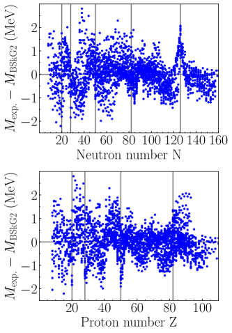
Figure 1: (Color online) Difference of masses calculated with BSkG2 and known values of Ref. Wan21 , as a function of neutron number (top panel) and as a function of proton number (bottom panel). Gray bands indicate the magic numbers.

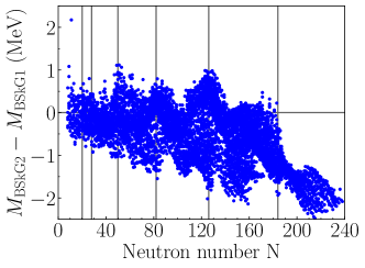
Figure 2: (Color online) Difference between masses obtained with BSkG1 and BSkG2 as function of neutron number. All nuclei $8\leq Z\leq 110$ that lie between the drip lines of both interactions are included. Gray vertical lines indicate the neutron magic numbers, including $N=184$.

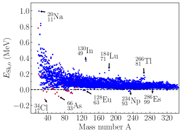
Figure 3: (Color online) Time-odd energy $E_{\rm Sk,o}$ as a function of mass number $A$ for all nuclei with odd neutron and/or proton number within the calculated drip lines. $N=Z$ nuclei are indicated in red, all others in blue. Some nuclei with particularly large or small time-odd energies are pointed out.

The contributions of the time-odd terms to the nuclear masses are shown in Fig. 3. Globally, the effects are small, although a few outliers can be seen. The largest contributions occur for light nuclei, with a global maximum of about 1 MeV for odd-odd ¹⁸Na. For heavy nuclei, the largest effects are on the order of 200 keV. Nevertheless, in all regions of the nuclear chart there are many nuclei for which the time-odd contribution to the energy is very small. For odd-odd nuclei, the average contribution of time-odd terms is about 100 keV while that for odd-mass nuclei is slightly more than half that, roughly 60 keV. The time-odd energy in even-$Z$, odd-$N$ nuclei is only slightly larger than that in odd-$Z$, even-$N$ nuclei with on average 65 keV and 50 keV, respectively. Averaged over all nuclei affected, odd-mass and odd-odd, the time-odd terms reduce the binding energy by about 70 keV. These averages hide significant variations, as can be seen in Fig. 3.

While the total time-odd energy is never very large, we note that the contributions of individual terms in the energy density need not be so small themselves, particularly for light nuclei. For ³⁴Cl for example, the total time-odd energy of about $-0.13$ MeV results from a cancellation between the contribution of spin terms (about +0.34 MeV) and the time-odd spin-orbit term (about $-0.42$ MeV) that are both a few times larger than the net effect. The current terms contribute very little for that nucleus.

A particularly striking aspect of Fig. 3 is that the total time-odd energy is almost always positive, i.e. it reduces the total binding energy in virtually all nuclei that it contributes to. This can be easily understood in terms of the coupling constants of these terms that are listed in Table 3. In both isospin channels, the coupling constant $C^{ss}_{t}$ of the density-independent term is large and positive, while the coupling constant of the density-dependent term $C^{ss\rho^{\gamma}}_{t}$ is of similar size but opposite sign. The net effect is that for all densities encountered in nuclei the spin terms are repulsive. On the one hand, this is consistent with empirical knowledge about collective spin- and spin-isospin response of nuclei, see Ref. Bender02 and references therein, but on the other hand it is also known that specific proton-neutron matrix elements of the spin terms have to be attractive in order to reproduce the empirical Gallagher-Moszkowski rule Robledo14 . The coupling constants $C^{j\nabla s}_{t}$ of the time-odd spin-orbit contributions are both negative, but they multiply an integral that can have either sign depending on the relative orientations of spin and orbital angular momenta of the nucleons. Similarly, the contribution of the current terms can be of either sign. It often will remain small, however. For odd-mass nuclei, the current terms are dominated by the contribution from the blocked particle, for which the strictly positive integral over $\mathbb{j}^{2}_{q}(\mathbb{r})$ is multiplied by the very small sum of coupling constants $C^{jj}_{0}+C^{jj}_{1}=-4.264\,\text{MeV}\,\text{fm}^{3}$. For odd-odd nuclei, the proton-neutron contribution will dominate as it is multiplied by the comparatively large difference $2\,(C^{jj}_{0}-C^{jj}_{1})=-38.554\,\text{MeV}\,\text{fm}^{3}$ of isoscalar and isovector coupling constants, but depending on the relative size and direction of the orbital angular momenta of the two blocked particles it multiplies an integral that can have either sign, such that this term is also not necessarily attractive. In any event, the coupling constants of the current terms remain smaller than those of the spin terms.

Table 3: Values of the isoscalar ($t=0$) and isovector ($t=1$) coupling constants of the time-odd terms in the Skyrme EDF (2.1.1) found for BSkG2. The $C^{ss}_{t}[n_{0}]$ are the effective spin-spin coupling constants at saturation density $n_{0}$, see A.

Coupling constant	$t=0$	$t=1$
$C^{ss}_{t}$ [MeV fm3]	$150.023$	$235.718$
$C^{ss\rho^{\gamma}}_{t}$ [MeV fm3+3γ]	$-205.152$	$-257.468$
$C^{ss}_{t}[n_{0}]$ [MeV fm3]	$32.153$	$87.791$
$C^{jj}_{t}$ [MeV fm5]	$-21.409$	$17.145$
$C^{j\nabla s}_{t}$ [MeV fm5]	$-81.478$	$-27.151$

Further trends can be found by more detailed inspection of Fig. 3. For instance, the effects of the time-odd terms are in general larger for nuclei with odd proton and odd neutron number than for odd-mass nuclei. Furthermore, the outliers with largest positive $E_{\rm Sk.,o}$ are odd-odd nuclei with both $N$ and $Z$ close to magic numbers. ¹³⁰In and ¹⁸⁴Lu are remarkable: in both cases the isovector current term is comparably large (roughly $100$ and $60$ keV respectively), due to the the large angular momenta of the odd proton and neutron oriented in opposite directions.

The size of the time-odd contribution to the nuclear binding energy and its trend with mass number is consistent with the existing literature on Skyrme parameterizations. The results of those that have been studied earlier, however, do not agree among each other. For some, the effect has been reported as being generally attractive, while for others it is generally repulsive or of varying sign. The comparison is also complicated by different groups having different strategies to choose the coupling constants of the spin terms that are not fixed by Galilean invariance Hellemans12 ; Bender02 ; Pototzky10 ; Schunck10 . By contrast, the size of coupling constants of the current terms is determined by the effective mass of the parameterization, as these terms are linked to the time-even $\rho_{t}\tau_{t}$-terms of Eq. (2.1.1) by Galilean invariance. For example, $C^{jj}_{0}$ will vanish for a parameterization with isoscalar effective mass $M^{*}_{s}/M=1.0$, and become increasingly negative when lowering $M^{*}_{s}/M$.

Our results are comparable to those of the large-scale HF+BCS study of odd nuclei with three Skyrme parameterizations reported in Ref. Pototzky10 : in particular the authors find that including the time-odd spin terms, as we do here, generally leads to a decrease in the total binding energy. The authors of Ref. Schunck10 find time-odd energies of about 100 keV in systematic calculations of both ground-state and excited states of odd-mass nuclei in the rare earth region. For different parameterizations and different treatments of time-odd terms, this effect can be either repulsive or attractive. Results for smaller sets of nuclei paint a similar picture; the time-odd terms of the popular SLy4 parameterization Chabanat98 lead to a decrease of binding energies of Ce isotopes by about 100-200 keV Duguet2001a , but to a few hundred keV for light nuclei Satula99 .

The overall situation is different for relativistic EDF models: for the ones that have been used in time-reversal-breaking calculations of odd- and odd-odd nuclei so far, the time-odd terms always increase the binding energy by about 100-300 keV, almost independent of the parameterization employed Afanasjev10a . The main difference to the non-relativistic approach that we use here is that the EDFs used in Ref. Afanasjev10a are constructed as Hartree models that target the time-even terms, and for which only those time-odd terms appear that are necessary to conserve the Lorentz-invariance of the EDF Vretenar05 . As a consequence, the time-odd sector of these models only contains current and spin-orbit terms, but no spin terms, as can be easily seen when constructing their non-relativistic limit Sulaksono07 . In fact, in order to describe spin- and spin-isospin response within these models, one is obliged to add additional phenomenological spin terms Paar04a that are not considered when calculating ground states. As relativistic EDF models all have comparatively low effective mass Vretenar05 , the isoscalar current terms fixed by Lorentz invariance are large and attractive, which explains the global energy gain from time-odd terms. Nevertheless, the overall size of the effect and its decrease with mass number compares well to our results. We are not aware of any systematic study of the effect of time-odd terms for EDFs of the Gogny type.

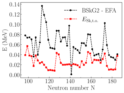
Figure 4: (Color online) Differences in $E_{\rm tot}$ as a function of neutron number for all bound odd-mass Pb isotopes between the complete calculation and a calculation employing the EFA (black circles). The total energy shift due to time-odd terms in the complete calculation (red squares) is also shown.

3.3 Quality of the equal filling approximation

We discuss in this section the quality of the EFA for absolute masses and their differences. We will distinguish between two effects here: (i) the direct contribution of the time-odd terms to the total binding energy and (ii) the polarisation effect, i.e. the change in the time-even part of the energy due to the presence of the time-odd mean-fields. We will visualize the direct effect by plotting the size of the time-odd terms and explore the second one by calculating mass differences between calculations employing the full EDF of Eq. (5) and those employing the EFA.

Figure 4 shows the difference in $E_{\rm tot}$ for all bound odd-mass Pb isotopes between the BSkG2 drip lines as a function of neutron number, as well as the time-odd contribution to the energy. First we note, as we already concluded from Fig. 3, that the EFA produces larger binding energies such that the difference plotted in Fig. 4 is positive across the entire isotopic chain. The time-odd terms show only a modest amount of variation with neutron number and remain small everywhere. The complete effect can be several times larger than just the contribution of the time-odd terms, but it remains on the level of about a hundred keV. Compared to the rms deviation of the model on the total masses, $\sigma(M)=0.668$ MeV, it seems unlikely the parameter adjustment was significantly influenced by the inclusion of the time-odd terms.

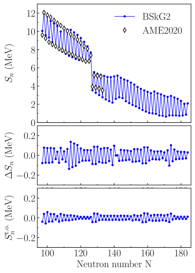
Figure 5: (Color online) Top panel: neutron separation energies $S_{n}$ along the Pb isotopic chain as calculated with BSkG2 up to the last neutron-bound isotope (blue circles) and as tabulated in AME2020 Wan21 (open diamonds). Middle panel: difference in neutron separation energies $\Delta S_{n}$ between full and EFA calculations. Bottom panel: contribution of the time-odd terms to the neutron separation energy, Eq. (17).

We show the calculated BSkG2 neutron separation energies for Pb isotopes in the top panel Fig. 5, as well as the data of AME2020. As expected from the global accuracy of the model, the reproduction of the experimental separation energies is quite good for isotopes up to the $N=126$ shell closure, while for the heavier ones their staggering is somewhat overestimated. Calculation in EFA result in a curve that is indistinguishable from the one shown on the top panel of Fig. 5. Instead, we show the difference between the complete and an EFA calculation, $\Delta S_{n}=S^{\rm BSkG2}_{n}-S^{\rm EFA}_{n}$, separately in the middle panel. The bottom panel of Fig. 5 shows the contribution of the time-odd terms to the neutron separation energies:

$$S^{\rm t.o.}_{n}(Z,N) =E_{\rm Sk,o}(Z,N-1)-E_{\rm Sk,o}(Z,N)\,.$$ (17)

As the time-odd terms are zero for even-even nuclei, for an even-even isotope this quantity equals the total time-odd Skyrme energy of its odd neighbor with one neutron less, while for an odd-mass isotope this is minus the time-odd Skyrme energy of the nucleus itself. When plotting this quantity, two consecutive values therefore have the same size, but opposite sign, which explains the symmetric pattern found in Fig. 5. A few things are readily apparent: first, the differences between complete and EFA calculations are small. Second, these differences always enhance the staggering between even and odd systems, i.e. they enlarge the separation energy for even-$N$ nuclei and reduce it for odd-$N$ nuclei. Third, the bare value of the time-odd energy is responsible for only roughly half of this effect; it accounts for a few tens of keV only, although its contribution is somewhat larger for lighter nuclei. The remaining part of the complete difference between EFA and complete calculations is therefore due to the polarising effect induced by the time-odd mean-fields. Fourth, all of these effects remain roughly constant in size for all values of $N$, although their relative importance changes: near the drip line the separation energies become smaller and hence the time-odd fields become comparatively more important. The smallest separation energy in Fig. 5 is about 660 keV for ²⁵³Pb, about 5% of which is due to the time-odd terms.

We show the effect of the inclusion of time-odd terms on the calculated five-point mass differences $\Delta^{(5)}_{n}$ of Eq. (16) in the top panel of Fig. 6 for the Pb isotopes. For the BSkG2 parameter set at least, accounting for time-reversal symmetry breaking results an increase of the value of the five-point gap between 5% and 10% compared to an EFA calculation, as shown on the bottom panel of Fig. 6. This increase remains constant from stability to the drip line. If one adjusts the pairing strength for a local study, i.e. limited to a handful of nuclei, an effect of this size can be meaningful. In the context of global calculations however, this difference is minor: a simple rescaling by a few percent will not bring the global models closer to the experimental data in a systematic way, as can clearly from the qualitative rather than quantitative agreement between calculated and experimental values for the neutron-deficient Pb isotopes in Fig. 6.

The authors of Ref. Pototzky10 report an effect on the gaps of comparable size, though whether they increase or decrease depends on the details of the treatment of the time-odd terms. A much larger effect for a relativistic approach was reported in Ref. Rutz99 for spherical Sn isotopes. There is a qualitative difference between these results and ours, though: As already mentioned above, the time-odd terms increases the binding energies of odd-mass nuclei in the relativistic approach of Ref. Rutz99 , such that at given pairing strength they decrease the pairing gaps, while in our calculations they increase the gaps. Conversely, to obtain a given value for the pairing gap, in the relativistic approach of Ref. Rutz99 one has to increase the pairing strength when including the effects of time-odd terms, whereas in ours the pairing strength has to be decreased. This can have a sizeable impact on many other observables.

A study employing a Gogny-type EDF found almost no effect on pairing gaps when including time-odd terms Robledo12 .

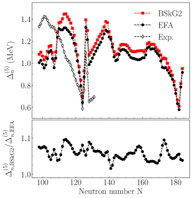
Figure 6: (Color online) Top panel: neutron five-point pairing gaps $\Delta^{(5)}_{n}$ along the Pb isotopic chain as calculated with BSkG2: the complete calculation (black circles) or when using the EFA (black circles). Experimental data was taken from AME2020 Wan21 (open diamonds). Bottom panel: ratio of the $\Delta^{(5)}_{n}$ from the complete and EFA calculations.

3.4 Pairing properties

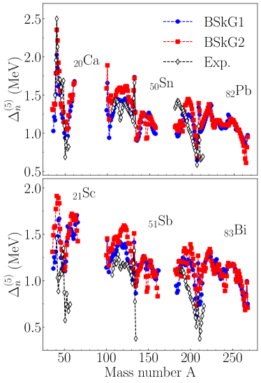
Figure 7: (Color online) Five-point neutron pairing gaps $\Delta_{n}^{(5)}$ for selected even-$Z$ isotopic chains (top panel: Ca, Sn, Pb) and neighbouring odd-$Z$ isotopic chains (bottom panel: Sc, Sb and Bi) obtained with BSkG1 (blue circles), BSkG2 (red squares) as well as experimental data (black triangles).

The top panel of Fig. 7 shows the five-point neutron gap $\Delta^{(5)}_{n}$ as defined in Eq. (16) for the even-$Z$ Ca ($Z=20$), Sn ($Z=50$) and Pb ($Z=82$) chains (top panel) as well as the odd-$Z$ Sc ($Z=21$), Sb ($Z=51$) and Bi ($Z=83$) chains (bottom panel). This quantity is generally indicative of the strength of pairing correlations in nuclei, but other effects such as time-odd terms (see the discussion around Fig. 6) and structural changes along the isotopic chain contribute as well Duguet2001a ; Bender00b ; Duguet2001b . For the even-$Z$ nuclei, the overall size of the gaps is very reasonably reproduced, but not all details of their evolution with neutron number. For example, the calculated gaps increase much quicker than the experimental ones when going away from the $N=82$ and $N=126$ neutron shell closures in the Sn and Pb chains, respectively, which for the latter could also be clearly seen on Fig. 6. In addition, the calculations miss some local features such as the dip observed near $A\simeq 115$ in the Sn isotopes and produce an arch-like structure around $A\simeq 195$ in the Pb isotopes that is not present in the experimental data. Many of these local differences can be expected to be related to imperfections in the description of the bunching of single-particle levels around the Fermi energy, rather than to deficiencies of the modelling of pairing. For neutron-rich Pb isotopes beyond $N=126$, the model appears to overestimate the neutron pairing gaps. The available data for the latter are limited however, such that it cannot be entirely ruled out that this large difference is an artifact from the already mentioned too quick increase of the gaps around shell closures. This quality of global reproduction is about typical for even-$Z$ nuclei across the nuclear chart and is entirely comparable to the performance of BSkG1. As already discussed in Ref. Scamps21 , this quality of description of nuclear pairing can only be achieved by controlling it in the parameter adjustment; we did so here by fitting the calculated average pairing gap to five-point differences, as explained in Sec. 2.4.1.

For odd-$Z$ chains, however, BSkG2 systematically overestimates the $\Delta^{(5)}_{n}$, as can be seen in the bottom panel of Fig. 7 for the examples of the Sc, Sb and Bi isotopic chains. The global trends of the $\Delta^{(5)}_{n}$ are very similar to the ones found for the Ca, Sn, and Pb chains, but compared to experiment the values are systematically higher. The same effect is also present for the proton gaps: experimental values are well-described for even-$N$ isotonic chains, but are somewhat too large for odd-$N$ chains. This deficiency is not a particularity of BSkG2: BSkG1 exhibits the same systematic effect. We do not interpret this mismatch between experiment and our models as a flaw of the adjustment of the pairing strengths but as the sign of a missing physical ingredient: in the BSkG models, we miss a mechanism to produce extra binding energy due to the residual interaction between the odd neutron and odd proton in odd-odd nuclei Jensen84 ; Friedman07 ; Wu16 . It is this additional binding energy which is thought to be at the origin of the observed systematic difference in three- or five-point gaps between both adjacent even-$Z$ and odd-$Z$ isotopic chains and adjacent even-$N$ and odd-$N$ isotonic chains. The microscopic-macroscopic approach of Ref. Moller16 includes a simple analytic term to account for this effect: adding such a contribution here would shift the calculated curves on the bottom panel of Fig. 7 downwards, improving our description of experiment. For the older BSk-models, this effect was partially mimicked by adopting different pairing strengths for even-even, odd-even, even-odd and odd-odd nuclei Goriely16 .

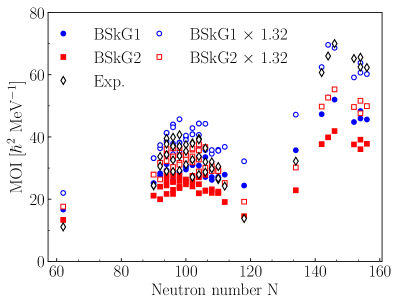
Figure 8: Belyaev moments of inertia (MOI) as a function of neutron number as obtained from BSkG1 and BSkG2 calculations (full blue circles and red squares, respectively). MOI multiplied with 1.32 are shown for both models as open symbols of the corresponding colors. These results are compared to experimental data for medium to heavy nuclei (open black diamonds) from Refs. Zeng94 ; Afanasjev00 ; Pearson91 .

Another quantity that is indicative of the pairing strength in nuclei are the rotational moments of inertia (MOI): this quantity becomes systematically smaller with increasing pairing strength, leading to a larger spread between energy levels in a rotational band Hellemans12 ; Belyaev61 . The Belyaev MOI for 48 even-even nuclei were included in the BSkG1 objective function as a means to control the pairing strengths for protons and neutrons. This approach is not entirely satisfactory: the Belyaev MOI captures only the perturbative first-order response to collective rotation and does not describe the entirety of the nucleus’ response to rotation as discussed in Sec. 2.3. As outlined in Sect. 2.3, the more reliable Thouless-Valatin approach to calculate the MOI systematically yields values that typically are larger than the Belyaev MOI by about $30\,\%$. Hence, a better way would be to include either a calculation of the Thouless-Valatin MOI in the objective function (which is computationally much more demanding) or rescale the Belyaev MOI with an ad-hoc factor (which adds a phenomenological ingredient to our model). Instead, we opted to drop the Belyaev MOI from the objective function, including the five-point gaps instead as (i) they are more directly connected to the neutron pairing strength and (ii) large amounts of experimental data is readily available.

In Fig. 8, we show the bare and rescaled Belyaev MOI for both BSkG1 and BSkG2. The bare BSkG1 values underestimate the experimental ones by about 10% for medium-heavy nuclei and an even larger percentage for actinide nuclei. Rescaling with the factor of 1.32 of Ref. Libert99 fixes the discrepancy for the actinides, but renders the MOI for rare-earth nuclei somewhat too large by about 20% on average. The Belyaev MOI calculated with BSkG2 are systematically smaller than the BSkG1 values. The bare values therefore significantly underestimate the experimental ones for all nuclei across the nuclear chart. The rescaled MOI obtained with BSkG2, however, agree quite well with data for nuclei in the rare-earth region. Like with BSkG1, however, data for medium-heavy and actinide nuclei are not described simultaneously with BSkG2 either.

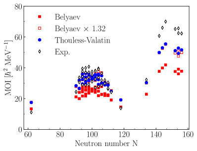
Figure 9: (Color online) Thouless-Valatin (blue circles), Belyaev (full red squares) and rescaled Belyaev (open red squares) moments of inertia obtained with BSkG2 for the nuclei already shown in Fig. 8. Experimental data (open black diamonds) from Refs. Zeng94 ; Afanasjev00 ; Pearson91 .

Having fixed the time-odd terms in the parameter fit of BSkG2, we also performed self-consistent cranking calculations minimizing the Routhian of Eq. (14) at the small rotational frequency of $\hbar\omega_{z}=0.01$ MeV for the same set of nuclei as shown in Fig. 8. For these calculations, we imposed an additional constraint to keep the quadrupole deformation of each nucleus fixed at its ground state value. We show the Thouless-Valatin MOI obtained in this way, as well as the Belyaev and rescaled Belyaev MOI in Fig. 9. The agreement between experiment and Thouless-Valatin MOI is rather good, again with the exception of the actinides. Altogether, these findings for the MOI indicate that the parameter adjustment of BSkG2 led to overall slightly smaller and thereby slightly more realistic effective pairing strengths than the ones of BSkG1, at least for not too heavy nuclei. We note though that the different values for $V_{\pi n}$ and $V_{\pi p}$ of BSkG1 and BSkG2 as listed in Tab. 1 are not directly indicative of the relative pairing strength of the models, as also the ratio $\eta$ between volume and surface contributions to the pairing energy is quite different.

Figure 9 also confirms that rescaling the Belyaev MOI by a factor 1.32 is a good approximation to the Thouless-Valatin MOI for the well-deformed nuclei with $\beta\geq 0.26$ that we consider here.

Figure 10: (Color online) Calculated quadrupole deformation $\beta$ (top panel) and triaxiality angle $\gamma$ (bottom panel) with BSkG1 (blue circles) and BSkG2 (red squares), compared to experimental information (open black diamonds). Top panel: quadrupole deformation $\beta$ with experimental information from Nudat nudat for ⁶⁶Zn Rocchini21 , ⁷⁰Ge Sugawara03 , ⁷²Ge Ayange16 , ⁷⁴Ge Toh00 , ⁷⁶Ge Ayange19 , ^74,76Kr Clement07 , ^76,80,82Se Kavka95 , ⁹⁸Sr Clement16 , ⁹⁶Mo ZielinskaPhD , ⁹⁸Mo Zielinska02 , ¹⁰⁰Mo Wrzosek12 , ¹⁰⁴Ru Srebrny06 , ¹¹⁰Cd Wrzosek20 , ¹¹⁴Cd Fahlander88 , ^106,108,110Pd Svensson95 , ¹³⁰Xe Morrison20 , ^{186,188,190,192}Os and ¹⁹⁴Pt Wu96 . Bottom panel: triaxiality angle $\gamma$, with experimental data points extracted from measured sets of transitional and diagonal $E2$ matrix elements Magda_priv for the same nuclei.

3.5 Shape: deformation and charge radii

The shapes of nuclear ground states predicted by BSkG2 are very similar to the ones obtained with BSkG1. The new model reproduces about equally well the global systematics of (total) quadrupole deformation of even-even nuclei as deduced from measured $B(E2)$ transition rates Raman01 . The systematics of nuclear charge radii also do not differ strongly between both models, as could have been expected from the comparable rms and mean deviations reported in Tab. 2. We have also found the more fine-grained evolution of the radii with neutron or proton number in many regions to be similar. Plots of deformation and charge radii compared to the experimental information on these quantities are close to Figs. 6 and 9 of Ref. Scamps21 , we omit them here.

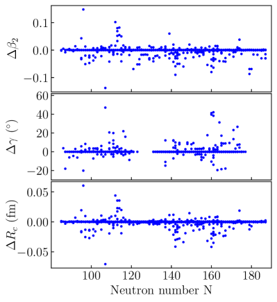
Figure 11: Difference in quadrupole deformation and rms charge radius between a complete calculation and one employing the EFA (full - EFA) for odd-mass and odd-odd nuclei with $76\leq Z\leq 88$ between the BSkG2 drip lines. Top panel: difference in $\beta$. Middle panel: difference in $\gamma$ for nuclei with $\beta\geq 0.1$. Bottom panel: difference in rms charge radius.

This similarity between the models also extends to triaxial deformation: Fig. 10 shows the total quadrupole deformation $\beta$ (top panel) and the triaxiality angle $\gamma$ (bottom panel) for 26 even-even nuclei. We compare (i) the calculated triaxiality angle with the mean value of $\gamma$ as obtained through the analysis of Coulomb excitation experiments Kumar72 ; Cline86 ; Magda_priv and (ii) the calculated deformation $\beta$ with data from Nudat nudat . For the heavier nuclei, and in particular the Os and Pt isotopes, both models yield almost identical results. For lighter nuclei, BSkG2 does not produce as large deformations for the two Kr isotopes, in better agreement with experiment than BSkG1. On the other hand, the $\gamma$ values calculated with BSkG2 for $A<80$ compare less favorably with experiment than those of BSkG1. With the limitations of this type of comparison in mind Scamps21 , we conclude that both models compare roughly equally well to the experimental data.

This discussion of the global aspects of deformation and radii makes one suspect that the polarisation due to the time-odd terms does not strongly modify the nuclear shape. In order to quantify this effect, we show in Fig. 11 the difference in nuclear shape due to the time-odd terms for 830 odd-mass and odd-odd nuclei with $76\leq Z\leq 88$. More precisely, we show the difference in total quadrupole deformation $\beta$ (top panel), triaxiality angle $\gamma$ (middle panel) and charge radius $R_{c}$ (bottom panel) between the complete calculation with time-odd terms included and another one employing the equal filling approximation.

The change in total deformation due to polarisation is generally speaking limited, with $\Delta\beta$ exceeding $0.05$ only for about twenty nuclei. Only three outliers show $|\Delta\beta|\geq 0.1$: ^177,187Tl and ¹⁹⁵Bi. All three lie in a region where multiple mean-field minima with different deformations but almost identical energies coexist; a small change in the conditions of the calculations (i.e. presence versus absence of time-odd polarisation) can have a large impact on the nuclear shape by inverting the order of the minima. Experimentally, this region of neutron-deficient isotopes with $Z\simeq 82$ is known for dramatic changes in charge radii with neutron number that are generally interpreted in terms of such closely-balanced minima Sels19 ; Barzakh21 . Changes in deformation in the top panel of Fig. 11 correspond one-to-one to changes in charge radius, as shown in the bottom panel. Note that a change $\Delta R_{c}$ of about $0.05$ fm in this region of the nuclear chart corresponds to a change in isotopic shift of about $0.25$ fm², which is about the size of the anomalous odd-even staggering in the neutron-deficient Hg isotopes Sels19 . Our conclusion is similar for the changes in triaxiality angle $\gamma$: few nuclei exhibit a change larger than $10^{\circ}$ between a complete calculation and one employing the EFA. Around $N=160$, a small clump of Tl and Bi isotopes stands out which change from nearly oblate to nearly prolate with $\Delta\gamma\approx 40^{\circ}$.

Table 4: Infinite nuclear matter properties for BSkG1 Scamps21 and BSkG2 parameterizations. See Refs. Goriely16 ; Margueron02 ; Chamel10 for the various definitions.

Properties	BSkG1	BSkG2
$k_{F}$ [fm]	$1.3280$	$1.3265$
$n_{0}$ [fm-3]	$0.1582$	$0.1577$
$a_{v}$ [MeV]	$-16.088$	$-16.070$
$J$ [MeV]	$32.0$	$32.0$
$L$ [MeV]	$51.7$	$53.0$
$M_{s}^{*}/M$	$0.860$	$0.860$
$M_{v}^{*}/M$	$0.769$	$0.773$
$K_{v}$ [MeV]	$237.8$	$237.5$
$K_{\text{sym}}$ [MeV]	$-156.4$	$-150.6$
$K^{\prime}$ [MeV]	$376.7$	$376.3$
$G_{0}$	$0.35$	$0.36$
$G_{0}^{\prime}$	$0.98$	$0.98$

3.6 Infinite nuclear matter properties

The nuclear matter properties of the BSkG1 and BSkG2 parameterizations are summarized in Table 4. We repeat that, for both models, the isoscalar effective mass $M_{s}^{*}/M$ and the symmetry energy $J$ were enforced during the parameter adjustment, while a reasonable value for the incompressibility $K_{\nu}$ was guaranteed by our choice of the density-dependence parameter $\gamma=0.3$ Chabanat97 . Additionally, the Fermi momentum $k_{F}$ was adjusted to qualitatively reproduce the global trend of charge radii.

The Landau parameters $G_{0}$ and $G^{\prime}_{0}$ represent the effective spin-spin interaction between nucleons at the Fermi surface of infinite symmetric matter. Their BSkG2 values being positive is a consequence of our finding that the spin terms are repulsive at all densities encountered in nuclei. Making the same assumptions as outlined in Sec. 2.1.1 for the time-odd terms, we obtain very similar values of the Landau parameters $G_{0}$ and $G_{0}^{\prime}$ for BSkG1. Including the time-odd sector in the parameter adjustment thus did not significantly impact the Landau parameters $G_{0}$ and $G^{\prime}_{0}$; both BSkG1 and BSkG2 values are compatible with the recommended values ($G_{0}=0.4,G^{\prime}_{0}=1.2$) of Ref. Bender02 .

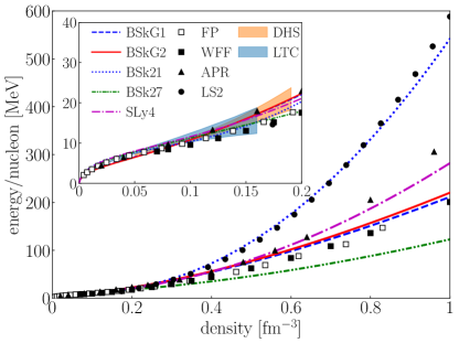
Figure 12: (Color online) Zero-temperature EOS for pure neutron matter with BSkG2, compared to ab-initio calculations referred to as FP, WFF, APR, LS2, DHS and LTC, as well as the BSkG1 Scamps21 , BSk21 Goriely10 , BSk27 Goriely13a and SLy4 Chabanat98 Skyrme parameterizations. FP corresponds to the calculation of Friedman & Pandharipande Friedman81 , WFF to “UV14 plus TNI” of Ref. Wiringa88 , APR of “A18 + $\delta\,v$ + UIX^∗" in Ref. Akmal98 and LS2 to V18 in Ref. Li08 . The bands labelled LTC and DHS refer to predictions based on chiral interactions from Refs. Lynn16 and Drischler19 respectively. The upper left insert is a zoom in view of densities below 0.2 fm^-3.

In Fig. 12, we compare the neutron matter equation of state (EOS) of BSkG2 with that predicted by other EDF-based models (BSkG1, BSk27, BSk21 and SLy4) and different types of ab-initio calculations. The BSkG2 EOS is virtually identical to the EOS predicted by BSkG1, and only at extreme densities a small difference is visible. This means that BSkG2 shares the qualities and flaws of BSkG1: at low densities the models fall just below the uncertainty bands of the recent chiral EFT-based predictions of Ref. Lynn16 and Ref. Drischler19 , see the inset of Fig. 12. At high densities the BSkG2 EOS is moderately stiff due to the enforced value of the symmetry energy $J=32$ MeV and qualitatively agrees with the WFF Wiringa88 and FP Friedman81 calculations, but is much less stiff than the LS2 prediction Li08 . Both the BSkG1 and BSkG2 models are intermediate in stiffness between BSk27 and BSk21 and close to the EOS obtained with SLy4 that itself has been adjusted to reproduce the “UV14+UVII” results of Ref. Wiringa88 . We note in particular that an EOS of moderate stiffness is at odds with the observation of massive pulsars like PSR J0740+66220 Fonseca21 .

We do not discuss explicitly other properties of unpolarised infinite nuclear matter, as BSkG1 and BSkG2 are nearly identical in these respects. In particular, we do not show the decomposition of the potential energy per nucleon among the four two-body spin-isospin $(S,T)$ channels, nor the neutron and proton effective masses in symmetric nuclear matter, as the resulting figures are virtually identical to Figs. 13 and 14 of Ref. Scamps21 . Calculations of polarised infinite neutron matter are discussed in Sec. 3.7.3.

3.7 Testing the time-odd terms

Time-odd terms also impact other quantities besides masses and the nuclear shape. We report here on some further benchmarks of the model for a limited amount of observables and nuclei. Aside from calculations with the BSkG2 parameterization as described above, we also employ three different variations of BSkG2 that have identical time-even parts but treat the time-odd channel differently:

• BSkG2_even: the BSkG2 parameterization with all time-odd coupling constants set to zero.

• BSkG2_GI: the BSkG2 parameterization with all coupling constants of the spin terms set to zero, but with current and time-odd spin-orbit terms unchanged.

• BSkG2_double: the BSkG2 parameterization with all coupling constants of the spin terms doubled, but with current and time-odd spin-orbit terms unchanged.

We remark that setting all time-odd coupling constants to zero implies that calculations with BSkG2_even are not Galilean invariant, and should hence be taken as purely illustrative. The two other parameterizations are manifestly Galilean invariant, as is BSkG2 itself.

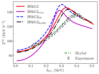
Figure 13: (Color online) Dynamical moment of inertia $\mathcal{I}^{(2)}$ as a function of cranking frequency $\hbar\omega_{z}$ for the superdeformed band of ¹⁹⁴Hg as calculated with BSkG2 and three variations (see text). These are compared the experimental ‘SD-1’ band of Ref. Singh02 (open diamonds) and the SLy5s1 results of Ref. Ryssens19b (green dash-dot-dotted line).

3.7.1 Superdeformed rotational band: ¹⁹⁴Hg

As a first example, we performed self-consistent cranking calculations of the superdeformed yrast band of ¹⁹⁴Hg (see Sec. 2.3). In Fig. 13, we compare BSkG2 results for the dynamical MOI $\mathcal{I}^{(2)}$ along this band to experimental information from Ref. Singh02 and the SLy5s1 results of Ref. Ryssens19b . Note that (i) we did not employ the semivariational strategy for these cranking calculations, treating the collective correction perturbatively and (ii) we employed the stabilisation procedure of Ref. Erler08 to avoid the disappearance of pairing correlations.

The unmodified BSkG2 parameterization offers a fair description of the rotational band, although it slightly underestimates the moment of inertia at low frequency and the maximum of the curve does not occur at the same location. The agreement with experiment is strictly worse than that obtained with the SLy5s1 parameterization, but we recall that (i) the pairing strengths used in Ref. Ryssens19b were optimized to describe superdeformed bands in this region Rigollet99 and (ii) we did not employ the Lipkin-Nogami procedure that was used in Ref. Ryssens19b . In fact, a calculation with SLy5s1 and the pairing strengths of Ref. Ryssens19b , but replacing the Lipkin-Nogami method with the same stabilisation procedure as used here, results in values for $\mathcal{I}^{(2)}$ (not shown) that are similar to those obtained with BSkG2.

Among all variants, only BSkG2_even produces results that are dramatically different from those of BSkG2: at low spin this parameterization severely underestimates the moment of inertia. Among the three Galilean-invariant parameterizations the differences are smaller, but enlarging the spin coupling constants (i) reduces slightly the moment of inertia at low angular momentum and (ii) moves the maximum of the curve towards higher frequencies, i.e. delays the onset of the quasiparticle alignment in the band. We note the value of the Belyaev MOI of the superdeformed configuration is $\mathcal{I}^{\rm B}\approx 67$ $\hbar^{2}$ MeV^-1. This value is about 25% lower of the Thouless-Valatin MOI, $\mathcal{I}^{\rm TV}\approx 86$ $\hbar^{2}$ MeV^-1, which is consistent with what has been found for the MOI of normal-deformed states in Sect. 3.4. The time-odd terms play a large role in this difference, as the Thouless-Valatin MOI for BSkG2_even is only about $73$ $\hbar^{2}$ MeV^-1.

Finally, these calculations serve the secondary purpose of testing the stability of the BSkG2 parameterization with respect to spurious finite-size instabilities Hellemans13 . The highest rotational frequencies shown in Fig. 13 correspond to large angular momenta of about $50\hbar$, hence to large spin and current densities. Even in such conditions, we have seen no sign of spurious finite-size instabilities in the spin channels.

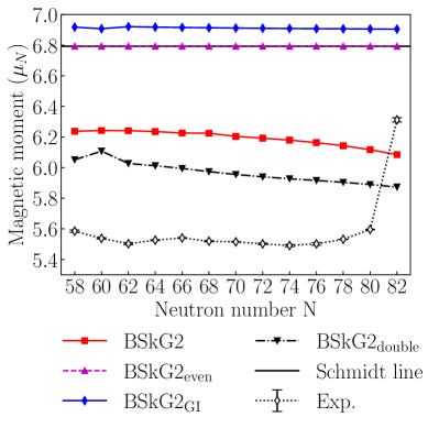
Figure 14: Magnetic moments of $\tfrac{9}{2}^{+}$ states in odd-mass In isotopes, calculated with BSkG2 and three variations (see text), as well as experimental data from Refs. Eberz87 and Vernon22 .

3.7.2 Magnetic moments: In isotopes

As second example of observables impacted by the time-odd terms, we study the magnetic moments of a limited set of nuclei. Following Bohr and Mottelson Bohr69 , the magnetic moment $\mu$ of a nucleus in a state with spin $J$ is defined as

$$\mu=\langle JM=J|\hat{M}_{1z}|JM=J\rangle\,,$$ (18)

where the expectation value is taken with respect to the substate with largest possible projection of the angular momentum $M=J$ on the $z-$axis in the laboratory frame. $\hat{M}_{1z}$ is the $z$-component of the $M1$ operator, that is given by

$$\hat{\boldsymbol{M}}_{1}=\sum_{i}\big{(}g_{\ell,i}\,\hat{\boldsymbol{\ell}}_{i}+g_{s,i}\,\hat{\mathbb{s}}_{i}\big{)}\,,$$ (19)

where $\hat{\mathbb{\ell}}_{i}$ and $\hat{\mathbb{s}}_{i}$ are the one-body operators for orbital and spin angular momentum, respectively. The $\hat{\boldsymbol{M}}_{1}$ operator is evidently time-odd and, when summed over all nucleons, probes the current ($\boldsymbol{\ell}$) and spin ($\boldsymbol{s}$) densities in the nuclear ground state. We take the bare values for the orbital and spin gyromagnetic factors of protons and neutrons:

$$g_{\ell,p} =\mu_{N}, g_{\ell,n} =0\,,$$ (20)

$$g_{s,p} =+5.586\mu_{N}, g_{s,n} =-3.826\mu_{N}\,,$$

where $\mu_{N}$ is the nuclear magneton.

For quasiparticle vacua that respect axial symmetry, it is possible to connect expectation values of $\hat{M}_{1}$ calculated in the intrinsic frame to the observed $\mu$, a quantity in the laboratory frame Bohr75 ; Bonneau15 ; Peru21 . For more general symmetry-broken states, there exists to the best of our knowledge no simple recipe to make the connection between both frames without resorting to full-fledged symmetry restoration approaches Sassarini21 ; Vernon22 ; Bally22 . Since our aim is an initial study of the effect of time-odd terms, we limited ourselves to one isotopic chain of (near-)spherical isotopes. In that simple case, the magnetic moment of the state with spin $J$ can be calculated directly from the quasiparticle vacuum $|\Phi\rangle$ as $\mu\approx\langle\Phi|\hat{M}_{1z}|\Phi\rangle$, provided this auxiliary state is constructed by blocking a quasiparticle with maximal alignment along the $z$-axis, i.e. whose angular momentum projection on the $z$-axis is close to $J$.

Motivated by recent experimental results Vernon22 , we selected the $J=\tfrac{9}{2}^{+}$ ground state of odd In ($Z=49$) isotopes as a testing ground. To construct near-spherical quasiparticle vacua, we (i) started the calculations from a carefully prepared spherically symmetric initial guess, (ii) used the direct diagonalization approach to the HFB problem to select a positive parity quasiparticle of the appropriate angular momentum near the Fermi energy at every iteration and (iii) used a cranking constraint, Eq. (14), to keep the total angular momentum along the $z$-axis equal to $\frac{9}{2}\hbar$. Finally, we did not execute a semivariational search for the minimum of $E_{\rm tot.}$, i.e. we took the correction energy $E_{\rm corr}$ as a perturbation.

In Fig. 14, we compare the magnetic moments obtained in this way with BSkG2 and its variants to experimental data from Refs. Vernon22 ; Eberz87 . From $N=58$ to $N=80$, the measured values show a quite strong and systematic deviation from the Schmidt line, which represents the magnetic moment of a non-interacting nucleon orbiting around a perfectly spherical core Schmidt34 . This reduction of the magnetic moment is generally taken to be a sign of current and spin distributions induced in the $Z=50$ core by the odd proton hole. The dramatic change of the magnetic moment for the heaviest isotope indicates that such polarisation is significantly less strong for a core with 82 neutrons.

A calculation with the original BSkG2 model leads to significant core polarisation, although not enough to match the experimental results. This polarisation is completely absent in a calculation with BSkG2_even, i.e. without time-odd terms, which matches exactly the Schmidt line. Considering only the coupling constants of time-odd terms dictated by Galilean invariance, we see that a small amount of polarization appears for BSkG2_GI though with the wrong sign, indicating that the spin terms induce most of the core polarisation found with the original BSkG2. Doubling the coupling constants of the spin terms enhances the polarisation further beyond the BSkG2 results.

While not being entirely satisfying, the overall level of agreement with data found for BSkG2 is similar, if not better than what is typically found for other (unaltered) parameterisations of the nuclear EDF Sassarini21 ; Bonneau15 ; Peru21 ; Vernon22 . To improve on the situation, it has recently been suggested to adjust the time-odd terms of Skyrme EDFs to experimental data on magnetic moments Sassarini21 ; Vernon22 . While our results in Fig. 14 confirm that varying the time-odd terms can resolve at least partially the tension with experiment, several questions remain to be solved before magnetic moments can be incorporated into large-scale models likes ours. First: what part of the observed polarisation should be reproduced by a symmetry-broken mean-field calculation? Given the constraints of a large-scale parameter adjustment, the symmetry restoration techniques used in Refs. Sassarini21 ; Vernon22 are likely out of reach for the immediate future. This question is particularly relevant in view of the dramatic difference between the magnetic moment of ¹³¹In and all other isotopes: BSkG2 and its variants produce smooth curves while symmetry-restored calculations with the UNEDF1 Skyrme parameterization are able to reproduce the discontinuity Vernon22 .

While probably a necessary ingredient of calculations of magnetic moments of the majority of deformed nuclei, from the few published studies it remains difficult to quantify the role and impact of symmetry-restoration for the description of the magnetic moments of spherical nuclei as the ones discussed here, and more analyses of the interplay of all modelling ingredients are clearly needed. For example, the calculations of Ref. Sassarini21 ; Vernon22 did not include pairing correlations; their absence can be expected to enhance core polarisation effects.

Finally, we mention that it is not entirely clear if Eq. (18) represents the entire $M1$ operator, as on very general grounds one can expect additional contributions from two-body currents Ericson88a and possibly other corrections from the consistent mapping of the full-many body problem onto an EDF approach, see the discussion in Ref. Bally22 and references therein. This issue is different from any empirical modification of the $g$-factors $g_{\ell/s}$ that could be justified by limitations of the model space employed. Since we treat all nucleons equally, instead of differentiating between a core and a valence space, we use the bare $g$-factors in Eq. (20).

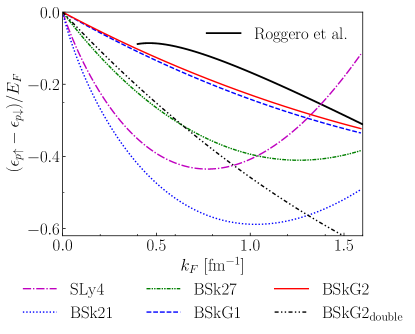
Figure 15: (Color online) Energy difference of between a spin-up and spin-down proton impurity in fully polarised neutron matter (see text) in units of the Fermi energy of the spin-up neutrons, and as a function of the Fermi momentum $k_{F}$. We show the predictions by the BSkG2 and BSkG2_double parameterization and by ab-initio calculations (full black line) of Ref. Roggero15 . For comparison, we also plot the predictions of the BSkG1 Scamps21 , BSk21 Goriely10 , BSk27 Goriely13a and SLy4 Chabanat98 Skyrme parameterizations.

3.7.3 Polarised neutron matter

All infinite matter constraints that impact the parameter adjustment concern unpolarized matter, whose properties only directly impact the time-even part of the functional. Recently, it has been suggested that ab-initio calculations of polarised neutron matter can be used to constrain the time-odd parts of the functional as well Roggero15 . A particular quantity that is affected only by the coupling constants of the time-odd terms in the EDF is the difference in the energy of a single spin-up and a single spin-down proton in a sea of of spin-up neutrons. We compare the predictions of several Skyrme parameterizations to the results of the ab-initio Monte Carlo calculations in Fig. 15. Although we did not constrain specifically the time-odd part of the EDF to reproduce this quantity, the BSkG1 and BSkG2 models are generally the closest to the ab-initio results. The BSkG2_double variant is wildly off and the BSkG2_even and BSkG2_GI variants result in zero energy difference between spin-up and spin-down impurities (curves not shown). As concluded in Ref. Roggero15 , it is clear that none of the parameterizations, including BSkG2, can reproduce even qualitatively the shape of the black full line, indicating the need to extend (the time-odd part of) the Skyrme EDF beyond the form we employ here.

4 Conclusion and outlook

4.1 Conclusion

We have presented a new entry in the series of Brussels-Skyrme-on-a-Grid (BSkG) models, which improves on the BSkG1 model of Ref. Scamps21 in two main ways. First: we removed the assumption of time-reversal symmetry and consistently employed the entire Skyrme EDF, including the time-odd terms. Second, we incorporated information on the fission properties of twelve actinide nuclei in the fitting protocol. The resulting model achieves an excellent description of ground-state properties with rms deviations of 0.668 MeV and 0.0274 fm on known masses and charge radii. Compared to the earlier BSkG1, the description of all observables entering the objective function slightly improves, such as the rms deviation of the AME2020 masses that is reduced by 63 keV. The infinite nuclear matter properties of the model remain close to those of BSkG1. BSkG2 reproduces reference values for primary and secondary fission barriers of 45 actinide nuclei with an rms deviation of 0.44 MeV and 0.47 MeV respectively, significantly improving on the BSkG1 deviations (0.88 MeV and 0.91 MeV, respectively). To the best of our knowledge, this is the best agreement with the reference data of RIPL-3 that is available in the literature; we will present our fission calculations in detail in a forthcoming paper Ryssens22 .

The parameter adjustment itself constitutes a major technical achievement: during the parameter adjustment we performed an enormous number of constrained Skyrme-HFB calculations for thousands of odd-mass and odd-odd nuclei with full inclusion of time-reversal breaking in 3D coordinate space. We managed to eliminate a large part of the convergence problems that plague this kind of calculations by using the gradient method to iterate the auxiliary states.

The changes brought by the time-odd terms to observables at fixed coupling constants have to be distinguished from the changes brought by the presence of the time-odd terms to the same observables after the readjustment of the parameters. For the majority of nuclei, switching the time-odd terms on for a given set of coupling constants changes the masses of odd- and odd-nuclei by a larger amount than the actual size of the time-odd terms, indicating sizeable polarization effects. In the parameter adjustment the change of binding energy brought by the presence of time-odd terms is then, however, counteracted for by changes of the other terms in the EDF.

For BSkG2, the total contribution of the time-odd terms to the masses of odd-mass and odd-odd nuclei is small (typically below 0.2 MeV in absolute value), although outliers for light nuclei can reach 1 MeV. These values are compatible with what has been observed in earlier studies, with the coupling constants of the time-odd terms also being fairly consistent with what is expected from phenomenology. Including or not the time-odd terms then typically alters separation energies by less than 200 keV, which for weakly-bound nuclei can, however, present a large relative change. When calculating five-point pairing gaps $\Delta^{(5)}$, including or not the time-odd terms, results in changes by $5$ to $10\%$. Nuclear deformation and charge radii are in general not strongly affected, although in exceptional situations the presence of the the time-odd terms can change the relative balance of coexisting minima. We have verified these conclusions across the entire nuclear chart, i.e. further than any previous study, and have established that these effects are roughly constant up to the neutron drip line. All of these results also present a large-scale benchmark of the EFA.

Since the overall effect of time-reversal symmetry breaking remains small, especially when compared to the typical deviation between calculations and experiment, the full inclusion of time-odd terms into the fitting procedure only leads to a small improvement of masses and mass differences compared to the use of the EFA as in BSkG1.

The effect of time-odd terms is not necessarily small for other quantities that are typically not included in large-scale parameter adjustments. We have illustrated the effect of time-odd terms on magnetic moments in In isotopes and on the superdeformed rotational band of ¹⁹⁴Hg. We have also compared our results to ab initio results for polarised infinite nuclear matter and shown the difference between Belyaev and Thouless-Valatin moments of inertia.

It should be kept in mind that our study chose one specific treatment for the time-odd terms that does not introduce additional free coupling constants. Other choices are possible, although the requirement of Galilean invariance will always link at least some of the time-odd terms to the time-even ones. Furthermore, we did not explore all possible orientations of the blocked quasiparticles. It seems unlikely however that modifying our treatment of time-odd terms or exploring more general nuclear configurations would alter any of our conclusions significantly.

4.2 Outlook

BSkG2 shares some of the weaknesses of BSkG1 already pointed out in Ref. Scamps21 . Both models predict only a relatively soft EOS for neutron matter, which is not compatible with the observation of pulsars of up to two solar masses. One possibility to remedy this issue without deteriorating the description of the properties of finite nuclei is to adopt the extended Skyrme form of Ref. Chamel09 .

Secondly, our treatment of correlation energy from rotational and vibrational motion remains schematic. Ideally, we should move beyond our symmetry-broken mean-field treatment and incorporate systematically symmetry restoration and configuration mixing techniques. Doing so requires both technical and formal developments. Technical work is necessary to make these techniques computationally feasible at the scale of the nuclear chart and in particular for systems with both even and odd numbers of nucleons. The formal challenge consists of finding a form of the Skyrme EDF based on multi-nucleon interactions which can rival the performance of the standard form using density dependent coupling constants Duguet09a . Simpler approaches can be tried first, to be used as stepping stones towards that ultimate goal. One such direction would be the use of the Thouless-Valatin rotational MOI in the collective correction, instead of the perturbative Belyaev MOI. With the current extension of our models to the time-odd sector, we can now access this MOI by way of self-consistent cranking calculations.

An issue of the BSkG1 and BSkG2 models we discovered during this work is our systematic overestimation of three- and five-point mass differences in odd-$Z$ isotopic and odd-$N$ isotonic chains, despite the quality of our description of the same quantity in adjacent chains with an even number of protons or neutrons, repectively.

Concerning the time-odd terms of the EDF: one could amend the fitting protocol with additional quantities that are sensitive to them, such as the magnetic moments and rotational MOI. Detailed preliminary studies are in our opinion indispensable, in particular to benchmark the size of beyond-mean-field effects. Time-odd observables are generally sensitive to the details of single-particle structure, meaning that it is not guaranteed that they can simultaneously be described in a global fashion using the standard form of the Skyrme EDF. In fact, that this is likely impossible can be deduced from Refs. Robledo14 ; Roggero15 : the traditional form fails to describe even qualitatively ab initio results for polarised neutron matter and often predicts relative spin orientations in ground states of odd-odd nuclei that are opposite to the empirical Gallagher-Mozkowski rules. Before attempting the construction of a new model, it would be desireable to establish a functional form that is better suited to satisfy these constraints.

Appendix A Coupling constants of $E_{\rm Sk}$

The Skyrme energy density $\mathcal{E}$ of Eq. (5) is determined by ten coupling constants, which are determined by the model parameters $t_{0-3},x_{0-3},W_{0}$ and $W_{0}^{\prime}$. The formulae relating these parameters to the coupling constants of the time-even part of the energy density were already presented in the appendices of Ref. Scamps21 . The coupling constants figuring in the time-odd part of the functional are

$$C^{ss}_{0} =-\tfrac{1}{4}t_{0}\left(\tfrac{1}{2}-x_{0}\right)\,,$$ (21a)

$$C^{ss}_{1} =-\tfrac{1}{8}t_{0}\,,$$ (21b)

$$C^{ss\rho^{\gamma}}_{0} =-\tfrac{1}{24}t_{3}\left(\tfrac{1}{2}-x_{3}\right)\,,$$ (21c)

$$C^{ss\rho^{\gamma}}_{1} =-\tfrac{1}{48}t_{3}\,,$$ (21d)

$$C^{jj}_{0} =-\tfrac{3}{16}t_{1}-\tfrac{1}{4}t_{2}\left(\tfrac{5}{4}+x_{2}\right)\,,$$ (21e)

$$C^{jj}_{1} =+\tfrac{1}{8}t_{1}\left(\tfrac{1}{2}+x_{1}\right)+t_{2}\left(\tfrac{1}{2}+x_{2}\right)\,,$$ (21f)

$$C^{j\nabla s}_{0} =-\frac{W_{0}}{2}-\frac{W_{0}^{\prime}}{4}\,,$$ (21g)

$$C^{j\nabla s}_{1} =-\frac{W_{0}^{\prime}}{4}\,.$$ (21h)

To facilitate the analysis of the effective sign and size of the spin-spin interaction at the densities encountered in nuclei and nuclear matter, it is useful to combine $C^{ss}_{t}$ and $C^{ss\rho^{\gamma}}_{t}$ into a density-dependent effective coupling constant Hellemans12 ; Bender02

$$C^{ss}_{t}[\rho_{0}]=C^{ss}_{t}+C^{ss\rho^{\gamma}}_{t}\,\rho_{0}^{\gamma}\,.$$ (22)

Appendix B Functional in the notation of Ref. Ryssens21

In Ref. Ryssens21 a new notation for local mean-field densities was developed to facilitate current and future efforts to generalize the form of the Skyrme functional. For various reasons, the numerical implementation of mean-field densities in MOCCa follows this new convention, instead of the more traditional notation of Sec. 2.1.1. To make the link with the practical implementation, we include here the formulation of both parts of the Skyrme energy, Eqs. (2.1.1) and (2.1.1), as well as the pairing energy, Eq. (9a), in the notation of Ref. Ryssens21 .

$$\mathcal{E}_{t,\rm e}(\mathbb{r}) =C^{\rho\rho}_{t}\,[D^{1,1}_{t}(\mathbb{r})]^{2}+C^{\rho\rho\rho^{\gamma}}_{t}[D^{1,1}_{0}(\mathbb{r})]^{\gamma}\,[D^{1,1}_{t}(\mathbb{r})]^{2}$$

$$+C^{\rho\tau}_{t}\,D^{1,1}_{t}(\mathbb{r})\,D^{(\nabla,\nabla)}_{t}(\mathbb{r})$$

$$+C^{\rho\Delta\rho}_{t}\,D^{1,1}_{t}(\mathbb{r})\,\Delta D^{1,1}_{t}(\mathbb{r})$$

$$+C^{\rho\nabla\cdot J}_{t}D^{1,1}_{t}(\mathbb{r})\,\boldsymbol{\nabla}\cdot\mathbb{C}^{1,\nabla\times\sigma}_{t}(\mathbb{r})\,,$$ (23)

$$\mathcal{E}_{t,\rm o}(\mathbb{r}) =C^{ss}_{t}\,\mathbb{D}^{1,\sigma}_{t}(\mathbb{r})\cdot\mathbb{D}^{1,\sigma}_{t}(\mathbb{r})$$

$$+C^{ss\rho^{\gamma}}_{t}\,[D^{1,1}_{0}(\mathbb{r})]^{\gamma}\,\mathbb{D}^{1,\sigma}_{t}(\mathbb{r})\cdot\mathbb{D}^{1,\sigma}_{t}(\mathbb{r})$$

$$+C^{jj}_{t}\,\mathbb{C}^{1,\nabla}_{t}(\mathbb{r})\cdot\mathbb{C}^{1,\nabla}_{t}(\mathbb{r})$$

$$+C^{j\nabla s}_{t}\,\mathbb{C}^{1,\nabla}_{t}(\mathbb{r})\cdot\nabla\times\mathbb{D}^{1,\sigma}_{t}(\mathbb{r})\,,$$ (24)

$$\mathcal{E}_{\rm pair}(\mathbb{r}) =\sum_{q=p,n}g_{q}(\mathbb{r})\,\Big{[}\tilde{D}_{q}^{1,1}(\mathbb{r})\,\tilde{D}_{q}^{1,1}(\mathbb{r})$$

$$\phantom{\sum_{q=p,n}g_{q}(\mathbb{r})\,\Big{[}}+\tilde{C}_{q}^{1,1}(\mathbb{r})\,\tilde{C}_{q}^{1,1}(\mathbb{r})\Big{]}\,,$$ (25)

where the functions $g_{q}(\mathbb{r})$ are defined in Eq. (9b). This notation unambiguously separates the time-even contribution $\propto\tilde{D}_{q}^{1,1}(\mathbb{r})\,\tilde{D}_{q}^{1,1}(\mathbb{r})$ to the pairing EDF from the time-odd contribution $\propto\tilde{C}_{q}^{1,1}(\mathbb{r})\,\tilde{C}_{q}^{1,1}(\mathbb{r})$.

Appendix C Explanation of the supplementary material

We provide as supplementary material the file
Mass_Table_BSkG2.dat, which contains the calculated ground state properties of all nuclei with $8\leq Z\leq 110$ lying between the proton and neutron drip lines. Its contents follows the same conventions as the supplementary material of Ref. Scamps21 , but we repeat the contents of the columns in Table. 5 for convenience. For clarity we mention that (i) we defined $M(N,Z)$ in Eq. (2) as the atomic mass, while columns 3 and 4 of the file list mass excesses and (ii) we report only the largest value among the three Belyaev MOIs $\mathcal{I}^{\rm B}_{x/y/z}$ in column 16.

Column	Quantity	Units	Explanation
1	Z	$-$	Proton number
2	N	$-$	Neutron number
3	$M_{\rm exp}$	MeV	Experimental atomic mass excess
4	$M_{\rm th}$	MeV	BSkG1 atomic mass excess
5	$\Delta M$	MeV	$M_{\rm exp}-M_{\rm th}$
6	$E_{\rm tot}$	MeV	Total energy, Eq. (1)
7	$\beta_{20}$	$-$	Quadrupole deformation
8	$\beta_{22}$	$-$
9	$\beta$	$-$
10	$E_{\rm rot}$	MeV	Rotational correction
11	$\langle\Delta\rangle_{n}$	MeV	Average neutron gap
12	$\langle\Delta\rangle_{p}$	MeV	Average proton gap
13	$r_{\rm BSkG2}$	fm	Calculated rms charge radius
14	$r_{\rm exp}$	fm	Experimental rms charge radius
15	$\Delta r$	fm	$r_{\rm exp}-r_{\rm BSkG2}$
16	$\mathcal{I}^{B}$	$\hbar^{2}$ MeV-1	Calculated Belyaev MOI.
17	par(p)	$-$	Parity of proton qp. excitation
18	par(n)	$-$	Parity of neutron qp. excitation

Table 5: Contents of the Mass_Table_BSkG2.dat file.

References

- (1) M. Arnould and S. Goriely, Astronuclear Physics: A tale of the atomic nuclei in the skies, Prog. Part. Nucl. Phys. 112, 103766 (2020).
- (2) H. Hergert, A Guided Tour of ab initio Nuclear Many-Body Theory, Frontiers in Physics 8, 379 (2020).
- (3) M. Bender, P.-H. Heenen, and P.-G. Reinhard, Self-consistent mean-field models for nuclear structure, Rev. Mod. Phys. 75, 121 (2003).
- (4) S. Goriely, N. Chamel, and J. M. Pearson, Further explorations of Skyrme-Hartree-Fock-Bogoliubov mass formulas. XVI. Inclusion of self-energy effects in pairing., Phys. Rev. C 93, 034337 (2016).
- (5) M. Dutra et al., Skyrme interaction and nuclear matter constraints, Phy. Rev. C 85, 035201 (2012).
- (6) M. Dutra et al., Relativistic mean-field hadronic models under nuclear matter constraints, Phys. Rev. C 90, 055203 (2014).
- (7) S. Goriely, S. Hilaire, M. Girod, and S. Péru, First Gogny-Hartree-Fock-Bogoliubov Nuclear Mass Model, Phys. Rev. Lett. 102, 242501 (2009).
- (8) D. Peña-Arteaga, S. Goriely, and N. Chamel, Relativistic mean-field mass models, Eur. Phys. J. A 52, 320 (2016).
- (9) S. Goriely, N. Chamel, and J. M. Pearson, Further explorations of Skyrme-Hartree-Fock-Bogoliubov mass formulas. XIII. The 2012 atomic mass evaluation and the symmetry coefficient, Phys. Rev. C 88, 061302(R) (2013).
- (10) P. Möller, A. J. Sierk, T. Ichikawa, and H. Sagawa, Nuclear ground-state masses and deformations: FRDM(2012), At. Data Nucl. Data Tables, 109, 1-204 (2016).
- (11) G. Scamps, S. Goriely, E. Olsen, M. Bender, and W. Ryssens, Skyrme-Hartree-Fock-Bogoliubov mass models on a 3D mesh: Effect of triaxial shape, Eur. Phys. J. A 57, 333 (2021).
- (12) W. Ryssens, Symmetry breaking in nuclear mean-field models, Ph.D. thesis, Université Libre de Bruxelles, (2016).
- (13) W. Ryssens, P.-H. Heenen, and M. Bender, Numerical accuracy of mean-field calculations in coordinate space, Phys. Rev. C 92, 064318 (2015).
- (14) L. M. Robledo and G. F. Bertsch, Global systematics of octupole excitations in even-even nuclei, Phys. Rev. C 84, 054302 (2011).
- (15) M. Chen, T. Li, J. Dobaczewski and W. Nazarewicz, Microscopic origin of reflection-asymmetric nuclear shapes, Phys. Rev. C 103, 034303 (2021).
- (16) T. Duguet, P. Bonche, P.-H. Heenen, and J. Meyer, Pairing correlations. I. Description of odd nuclei in mean-field theories, Phys. Rev. C 65, 014310 (2001).
- (17) V. Hellemans, P.-H. Heenen, and M. Bender, Tensor part of the Skyrme energy density functional. III. Time-odd terms at high spin, Phys. Rev. C 85, 014326 (2012).
- (18) J. A. Maruhn, P.-G. Reinhard, P. D. Stevenson, and M. R. Strayer, Spin-excitation mechanisms in Skyrme-force time-dependent Hartree-Fock calculations, Phys. Rev. C 74, 027601 (2006).
- (19) M. Bender, J. Dobaczewski, J. Engel, and W. Nazarewicz, Gamow-Teller strength and the spin-isospin coupling constants of the Skyrme energy functional, Phys. Rev. C 65, 054322 (2002).
- (20) M. Kortelainen, N. Hinohara, and W. Nazarewicz, Multipole modes in deformed nuclei within the finite amplitude method, Phys. Rev. C 92, 051302 (2015).
- (21) P. Bonche, J. Dobaczewski, H. Flocard, P.-H. Heenen, and J. Meyer, Analysis of the generator coordinate method in a study of shape isomerism in 194Hg, Nucl. Phys. A 510, 466 (1990).
- (22) N. Hinohara, T. Nakatsukasa, M. Matsuo, and K. Matsuyanagi, Effects of time-odd components in mean field on large amplitude collective dynamics, Prog. Theoret. Phys. 115, 567, (2006)
- (23) P. Klüpfel, Skyrme’s Interaction Beyond the Mean-Field: The DGCM+GOA Hamiltonian of Nuclear Quadrupole Motion, Thesis, Friedrich-Alexander-Universität Erlangen-Nürnberg (2008).
- (24) K. Petrík and M. Kortelainen, Thouless-Valatin rotational moment of inertia from linear response theory, Phys. Rev. C 97, 034321 (2018).
- (25) K. Washiyama, N. Hinohara, and T. Nakatsukasa, Finite-amplitude method for collective inertia in spontaneous fission, Phys. Rev. C 103, 014306 (2021).
- (26) P. Bonche, H. Flocard, and P.-H. Heenen, Self-consistent calculation of nuclear rotations: The complete yrast line of 24Mg, Nucl. Phys. A 467, 115-135 (1987).
- (27) J. Dobaczewski and J. Dudek, Time-odd rotating superdeformed nuclei, Phys. Rev. C 52, 1827 (1995).
- (28) L. M. Robledo, R. N. Bernard, and G. F. Bertsch, Spin constraints on nuclear energy density functionals, Phys. Rev. C 89, 021303 (2014).
- (29) P. L. Sassarini, J. Dobaczewski, J. Bonnard, and R. F. G. Ruiz, Global analysis of electromagnetic moments in odd near doubly magic nuclei, arxiv.org/abs/2111.04675.
- (30) D. Peña Arteaga, M. Grasso, E. Khan, and P. Ring, Nuclear structure in strong magnetic fields: Nuclei in the crust of a magnetar, Phys. Rev. C 84, 045806 (2011).
- (31) J. Margueron, J. Navarro, and N. Van Giai, Instabilities of infinite matter with effective Skyrme-type interactions, Phys. Rev. C 66, 014303 (2002).
- (32) N. Chamel, S. Goriely and J. M. Pearson, Further explorations of Skyrme-Hartree-Fock-Bogoliubov mass formulas. XI. Stabilizing neutron stars against a ferromagnetic collapse, Phys. Rev. C 80, 065804 (2009).
- (33) N. Chamel and S. Goriely, Spin and spin-isospin instabilities in asymmetric nuclear matter at zero and finite temperatures using Skyrme functionals, Phys. Rev. C 82, 045804 (2010).
- (34) L.-G. Cao, G. Colò, and H. Sagawa, Spin and spin-isospin instabilities and Landau parameters of Skyrme interactions with tensor correlations, Phys. Rev. C 81, 044302 (2010).
- (35) A. Pastore, D. Davesne, K. Bennaceur, J. Meyer, and V. Hellemans, Fitting Skyrme functionals using linear response theory, Phys. Scr. T154, 014014 (2013).
- (36) A. Pastore, D. Tarpanov, D. Davesne, and J. Navarro, Spurious finite-size instabilities in nuclear energy density functionals: Spin channel, Phys. Rev. C 92, 024305 (2015).
- (37) K. J. Pototzky, J. Erler, P.-G. Reinhard, and V. O. Nesterenko, Properties of odd nuclei and the impact of time-odd mean fields: A systematic Skyrme-Hartree-Fock analysis, Eur. Phys. J. A 46, 299-313 (2010).
- (38) A. V. Afanasjev, and H. Abusara, Time-odd mean fields in covariant density functional theory: Nonrotating systems, Phys. Rev. C 81, 014309 (2010).
- (39) S. Perez-Martin and L. M. Robledo, Microscopic justification of the equal filling approximation, Phys. Rev. C 78, 014304 (2008).
- (40) N. Schunck et al., One-quasiparticle states in the nuclear energy density functional theory, Phys. Rev. C 81, 024316 (2010).
- (41) S. Goriely, M. Samyn, and J. M. Pearson, Further explorations of Skyrme-Hartree-Fock-Bogoliubov mass formulas. VII. Simultaneous fits to masses and fission barriers, Phys. Rev. C 75, 064312 (2007).
- (42) W. Ryssens, G. Scamps, S. Goriely, and M. Bender, Skyrme-Hartree-Fock-Bogoliubov mass models on a 3D mesh: fission barriers with BSkG2, in preparation.
- (43) D. Lunney, J. M. Pearson, and C. Thibault, Recent trends in the determination of nuclear masses., Rev. Mod. Phys. 75, 1021-1082 (2003).
- (44) M. Wang et al., The AME 2020 atomic mass evaluation (II). Tables, graphs and references, Chin. Phys. C 45, 030003 (2021).
- (45) S. J. Krieger, P. Bonche, H. Flocard, P. Quentin, and M. S. Weiss, An improved pairing interaction for mean field calculations using Skyrme potentials, Nucl. Phys. A 517, 275 (1990).
- (46) S. Goriely and J. M. Pearson, Further explorations of Skyrme-Hartree-Fock-Bogoliubov mass formulas. VIII. Role of Coulomb exchange, Phys. Rev. C 77, 031301 (2008).
- (47) M. Bender, K. Rutz, P.-G. Reinhard, and J. A. Maruhn, Consequences of the center-of-mass correction in nuclear mean-field models, Eur. Phys. J. A 7, 467-478 (2000).
- (48) F. Tondeur, S. Goriely, J. M. Pearson, and M. Onsi, Towards a Hartree-Fock mass formula, Phys. Rev. C 62, 024308 (2000).
- (49) S. Goriely, N. Chamel, and J. M. Pearson, Further explorations of Skyrme-Hartree-Fock-Bogoliubov mass formulas. XIII. The 2012 atomic mass evaluation and the symmetry coefficient, Phys. Rev. C 88, 024308 (2013).
- (50) S. Goriely, M. Samyn, M. Bender, and J. M. Pearson, Further explorations of Skyrme-Hartree-Fock-Bogoliubov mass formulas. II. Role of the effective mass, Phys. Rev. C 68, 054325 (2003).
- (51) W. Ryssens, M. Bender and P.-H. Heenen, Iterative approaches to the self-consistent nuclear energy density functional problem: Heavy ball dynamics and potential preconditioning, Eur. Phys. J. A 55, 93 (2019).
- (52) M. M. Sharma, G. Lalazissis, J. König, and P. Ring, Isospin Dependence of the Spin-Orbit Force and Effective Nuclear Potentials, Phys. Rev. Lett. 74, 3744-3747 (1995).
- (53) P.-G. Reinhard and H. Flocard, Nuclear effective forces and isotope shifts, Nucl. Phys. A 584, 467-488 (1995).
- (54) T. Lesinski, M. Bender, K. Bennaceur, T. Duguet, and J. Meyer, Tensor part of the Skyrme energy density functional: Spherical nuclei, Phys. Rev. C 76, 014312 (2007).
- (55) P. Klüpfel, P.-G. Reinhard, T. J. Bürvenich, and J. A. Maruhn, Variations on a theme by Skyrme: A systematic study of adjustments of model parameters, Phys. Rev. C 79, 034310 (2009).
- (56) M. Kortelainen et al., Nuclear energy density optimization, Phys. Rev. C 82, 024313 (2010).
- (57) M. Kortelainen et al., Nuclear energy density optimization: Shell structure, Phys. Rev. C 89, 054314 (2014).
- (58) S. Goriely, Further explorations of Skyrme–Hartree–Fock–Bogoliubov mass formulas. XV: The spin-orbit coupling, Nucl. Phys. A 933, 68-81 (2015).
- (59) D. Davesne, A. Pastore, and J. Navarro, Linear response of homogeneous nuclear matter with energy density functionals, Phys. Rep. 563, 1 (2015).
- (60) V. Hellemans et al., Spurious finite-size instabilities in nuclear energy density functionals, Phys. Rev. C 88, 064323 (2013).
- (61) D. Davesne, A. Pastore, and J. Navarro, Linear response theory with finite-range interactions, Prog. Part. Nucl. Phys. 120, 103870 (2021).
- (62) M. Martini, A. De Pace, and K. Bennaceur, Spurious finite-size instabilities with Gogny-type interactions, Eur. Phys. J. A 55, 150 (2019).
- (63) C. Gonzalez-Boquera, M. Centelles, X. Viñas, and L. M. Robledo, Finite-size instabilities in finite-range forces, Phys. Rev. C 103, 064314 (2021).
- (64) E. Perlińska, S. G. Rohoziński, J. Dobaczewski, and W. Nazarewicz, Local density approximation for proton-neutron pairing correlations: Formalism, Phys. Rev. C 69, 014316 (2004).
- (65) S. T. Belyaev, Concerning the calculation of the nuclear moment of inertia, Nucl. Phys. 24, 322-325 (1961).
- (66) D. Baye and P.-H. Heenen, Generalised meshes for quantum mechanical problems, J. Phys. A. Math. Gen. 19, 2041 (1986).
- (67) J. Dobaczewski, J. Dudek, S. G. Rohoziński, and T. R. Werner, Point symmetries in the Hartree-Fock approach. I. Densities, shapes, and currents, Phys. Rev. C 62, 014310 (2000).
- (68) E. P. Wigner, Normal form of antiunitary operators., J. Math. Phys. 1, 409-413 (1960).
- (69) B. Banerjee, P. Ring, and H. J. Mang, On the character of the Hartree-Fock-Bogoliubov solutions in a rotating frame, Nucl. Phys. A 221, 564-572 (1974).
- (70) P. Ring and P. Schuck, The Nuclear Many-Body Problem, (Springer Verlag, 1980).
- (71) G. Bertsch, J. Dobaczewski, W. Nazarewicz, and J. Pei, Hartree-Fock-Bogoliubov theory of polarized Fermi systems, Phys. Rev. A 79, 043602 (2009).
- (72) M. Bender, N. Schunck, J.-P. Ebran, and T. Duguet, Chapter 3: Single-Reference and Multi-Reference Formulation, In Energy Density Functional Methods for Atomic Nuclei, Nicolas Schunck [ed.], IoP Publishing Ltd (2019).
- (73) P.-H. Heenen, P. Bonche, and H. Flocard, Microscopic study of superdeformation in 193Hg, Nucl. Phys. A 588, 490-500 (1995).
- (74) J. Dobaczewski et al., Solution of the Skyrme-Hartree-Fock-Bogolyubov equations in the Cartesian deformed harmonic-oscillator basis. (VI) hfodd (v2.40h): A new version of the program, Comp. Phys. Comm. 180, 2361-2391 (2009).
- (75) R. N. Perez, N. Schunck, R.-D. Lasseri, C. Zhang, and J. Sarich, Axially deformed solution of the Skyrme-Hartree-Fock-Bogolyubov equations using the transformed harmonic oscillator basis (III) hfbtho (v3.00): A new version of the program, Comp. Phys. Comm. 220, 363-375 (2017).
- (76) N. D. Woods, M. C. Payne, and P. J. Hasnip, Computing the self-consistent field in Kohn–Sham density functional theory, J. Phys. Condens. Matter 31, 453001 (2019).
- (77) J. L. Egido, J. Lessing, V. Martin, and L. M. Robledo, On the solution of the Hartree-Fock-Bogoliubov equations by the conjugate gradient method, Nucl. Phys. A 594, 70-86 (1995).
- (78) L. M. Robledo and G. F. Bertsch, Application of the gradient method to Hartree-Fock-Bogoliubov theory, Phys. Rev. C 84, 014312 (2011).
- (79) B. Gall, P. Bonche, J. Dobaczewski, H. Flocard, and P.-H. Heenen, Superdeformed rotational bands in the mercury region. A cranked Skyrme-Hartree-Fock-Bogoliubov study, Z. Phys. A 348, 183-197 (1994).
- (80) W. Ryssens, M. Bender, K. Bennaceur, P.-H. Heenen, and J. Meyer, Impact of the surface energy coefficient on the deformation properties of atomic nuclei as predicted by Skyrme energy density functionals, Phys. Rev. C 99, 044315 (2019).
- (81) C. J. Gallagher and S. A. Moszkowski, Coupling of angular momenta in odd-odd nuclei, Phys. Rev. 111, 1282-1290 (1958).
- (82) J. P. Boisson, R. Piepenbring, and W. Ogle, The effective neutron-proton interaction in rare-earth nuclei, Phys. Rep. 26, 99-147 (1978).
- (83) D. J. Thouless and J. G. Valatin, Time-dependent Hartree-Fock equations and rotational states of nuclei, Nucl. Phys. 31, 211-230 (1962).
- (84) N. Hinohara, Collective inertia of the Nambu-Goldstone mode from linear response theory, Phys. Rev. C 92, 034321 (2015).
- (85) J. Libert, M. Girod, and J. P. Delaroche, Microscopic descriptions of superdeformed bands with the Gogny force: Configuration mixing calculations in the A 190 mass region, Phys. Rev. C 60, 054301 (1999).
- (86) A. Bohr and B. R. Mottelson, Single-Particle and Collective Aspects of Nuclear Rotation, Phys. Scr. 24, 71-76 (1981).
- (87) J. Dudek, Nuclear superdeformation at high spins, Prog. Part. Nucl. Phys. 28, 131-185 (1992).
- (88) B. Singh, R. Zywina and R. B. Firestone, Table of Superdeformed Nuclear bands and Fission Isomers, Nucl. Data Sheets 97, 241-592 (2002).
- (89) S. Goriely, N. Samyn, and J. M. Pearson, Further explorations of Skyrme-Hartree-Fock-Bogoliubov mass formulas; VI: Weakened pairing, Nucl. Phys. A 773, 279 (2006).
- (90) M. Bender, K. Rutz, P.-G. Reinhard, and J. A. Maruhn, Pairing gaps from nuclear mean-field models, Eur. Phys. J. A, 8, 59-75 (2000).
- (91) T. Duguet, P. Bonche, P.-H. Heenen, and J. Meyer, Pairing correlations. II. Microscopic analysis of odd-even mass staggering in nuclei, Phys. Rev. C 65, 014311 (2001).
- (92) R. Capote et al., RIPL - Reference Input Parameter Library for Calculation of Nuclear Reactions and Nuclear Data Evaluation, Nucl. Data Sheets 110, 3107-3214 (2009).
- (93) E. Chabanat, P. Bonche, P. Haensel, J. Meyer and R. Schaeffer, A Skyrme parametrization from subnuclear to neutron star densities., Nucl. Phys. A 627, 710 (1997).
- (94) G. Colò, N. V. Giai, J. Meyer, K. Bennaceur, and P. Bonche, Microscopic determination of the nuclear incompressibility within the nonrelativistic framework, Phys. Rev. C 70, 024307 (2004).
- (95) L. G. Cao, U. Lombardo, and P. Schuck, Screening effects in superfluid nuclear and neutron matter within Brueckner theory, Phys. Rev. C 74, 064301 (2006).
- (96) W. Zuo, A. Lejeune, U. Lombardo, and J.-F. Mathiot, Interplay of three-body interactions in the EOS of nuclear matter, Nucl. Phys. A 706, 418 (2002).
- (97) I. Angeli and K. P. Marinova, Table of experimental nuclear ground state charge radii: An update, At. Data Nucl. Data Tables 99, 69 (2013).
- (98) R. Jodon, M. Bender, K. Bennaceur, and J. Meyer, Constraining the surface properties of effective Skyrme interactions, Phys. Rev. C 94, 024335 (2016).
- (99) Ph. Da Costa, M. Bender, K. Bennaceur, J. Meyer, and W. Ryssens, in preparation.
- (100) A. Mamdouh, J. M. Pearson, M. Rayet, and F. Tondeur, Fission barriers of neutron-rich and superheavy nuclei calculated with the ETFSI method, Nuc. Phys. A 679, 337-358 (2001).
- (101) S. A. Giuliani, G. Martínez-Pinedo, and L. M. Robledo, Fission properties of superheavy nuclei for r-process calculations, Phys. Rev. C 97, 034323 (2018).
- (102) E. Chabanat, P. Bonche, P. Haensel, J. Meyer, and R. Schaeffer, A Skyrme parametrization from subnuclear to neutron star densities Part II. Nuclei far from stabilities, Nucl. Phys. A635, 231 (1998).
- (103) W. Satuła, Wigner energy, odd-even mass staggering and the time-odd mean-fields, AIP Conference Proceedings 141, 141-150 (1999).
- (104) D. Vretenar, A. V. Afanasjev, G. A. Lalazissis, and P. Ring, Relativistic Hartree-Bogoliubov theory: Static and dynamic aspects of exotic nuclear structure, Phys. Rep. 409, 101-259 (2005).
- (105) A. Sulaksono, P.-G. Reinhard, T. J. Bürvenich, P. O. Hess, and J. A. Maruhn, From self-consistent covariant Effective Field Theories to their Galilean-invariant counterparts, Phys. Rev. Lett. 98, 262501 (2007).
- (106) N. Paar, T. Nikšić, D. Vretenar, and P. Ring, Quasiparticle random phase approximation based on the relativistic Hartree-Bogoliubov model. II. Nuclear spin and isospin excitations, Phys. Rev. C 69, 054303 (2004).
- (107) K. Rutz, M. Bender, P.-G. Reinhard, and J. A. Maruhn, Pairing gap and polarisation effects, Phys. Lett. B 468, 1-6 (1999).
- (108) L. M. Robledo, R. Bernard, and G. F. Bertsch, Pairing gaps in the Hartree-Fock-Bogoliubov theory with the Gogny D1S interaction, Phys. Rev. C 86, 064313 (2012).
- (109) A. S. Jensen, P. G. Hansen, and B. Jonson, New mass relations and two- and four-nucleon correlations, Nucl. Phys. A 431, 393-418 (1984).
- (110) W. A. Friedman and G. F. Bertsch, Neutron-proton pairing reexamined, Phys. Rev. C 76, 057301 (2007).
- (111) Z. Wu, S. A. Changizi, and C. Qi, Empirical residual neutron-proton interaction in odd-odd nuclei, Phys. Rev. C 93, 034334 (2016).
- (112) J. Y. Zeng, T. H. Jin, and Z. J. Zhao, Blocking effect and odd-even differences in the moments of inertia of rare-earth nuclei, Phys. Rev. C 50, 1388 (1994).
- (113) A. V. Afanasjev, J. König, P. Ring, L. M. Robledo, and J. L. Egido, Moments of inertia of nuclei in the rare earth region: A relativistic versus nonrelativistic investigation, Phys. Rev. C 62, 054306 (2000).
- (114) J. M. Pearson, Y. Aboussir, A. K. Dutta, R. C. Nayak, M. Farine, and F. Tondeur, Thomas-Fermi approach to nuclear mass formula, Nucl. Phys. A 528, 1 (1991).
- (115) National Nuclear Data Center, Nuclear structure and decay data on-line library, Nudat 2.8, 2018. https://www.nndc.bnl.gov/nudat2/.
- (116) M. Rocchini et al., Onset of triaxial deformation in 66Zn and properties of its first excited state studied by means of Coulomb excition, Phys. Rev. C 103, 014311 (2021).
- (117) M. Sugawara et al., Multiple Coulomb excitation of a 70Ge beam and the interpretation of the state as a deformed intruder, Eur. Phys. J. A 16, 409 (2003).
- (118) A. D. Ayangeakaa et al., Shape coexistence and the role of axial asymmetry in 72Ge, Phys. Lett. B 754, 254 (2016).
- (119) Y. Toh et al., Coulomb excitation of 74Ge beam, Eur. Phys. J. A 9, 353 (2000).
- (120) A. D. Ayangeakaa et al., Evidence for rigid triaxial deformation in 76Ge from a model-independent analysis, Phys. Rev. Lett. 123, 102501 (2019).
- (121) E. Clément et al., Shape coexistence in neutron-deficient krypton isotopes, Phys. Rev. C 75, 054313 (2007).
- (122) A. E. Kavka et al., Coulomb excitation of 76,80,82Se, Nucl. Phys. A 593, 177 (1995).
- (123) E. Clément et al., Spectroscopic quadrupole moments in 96-98Sr: evidence for shape coexistence in neutron-rich Strontium isotopes at , Phys. Rev. C 94, 054326 (2016).
- (124) M. Zielińska, Electromagnetic structure of molybdenum isotopes studied using Coulomb excitation method, Ph.D. thesis, Warsaw University, (2005).
- (125) M. Zielińska et al., Electromagnetic structure of 98Mo, Nucl. Phys. A 712, 3 (2002).
- (126) K. Wrzosek-Lipska et al., Electromagnetic properties of 100Mo: Experimental results and theoretical description of quadrupole degrees of freedom, Phys. Rev. C 86, 064305 (2012).
- (127) J. Srebrny et al., Experimental and theoretical investigations of quadrupole collective degrees of freedom in 104Ru, Nucl. Phys. A 766, 25 (2006).
- (128) K. Wrzosek-Lipska et al., Quadrupole Deformation of 110Cd studied with coulomb excitation, Acta Phys. Pol. B 51, 789 (2020).
- (129) C. Fahlander et al., Quadrupole collective properties of 114Cd, Nucl. Phys. A 485, 327 (1988).
- (130) L. E. Svensson et al., Multiphonon vibrational states in 106,108Pd, Nucl. Phys. A 584, 547 (1995).
- (131) L. Morrison et al., Quadrupole deformation of 130Xe measured in a Coulomb-excitation experiment, Phys. Rev. C 102, 054304 (2020).
- (132) C. Y. Wu et al., Quadrupole collectivity and shapes of Os-Pt nuclei, Nucl. Phys. A 607, 178 (1996).
- (133) M. Zielinska, private communication.
- (134) S. Raman, C. W. Nestor, and P. Tikkanen, Transition probability from the ground to the first-excited state of even-even nuclides, At. Data Nucl. Data Tables, 78, 1 (2001).
- (135) K. Kumar, Intrinsic quadrupole moments and shapes of nuclear ground states and excited states, Phys. Rev. Lett. 28, 249 (1972).
- (136) D. Cline, Nuclear shapes studied by Coulomb excitation, Ann. Rev. Nucl. Part. Sci. 36, 683 (1986).
- (137) S. Sels et al., Shape staggering of midshell mercury isotopes from in-source laser spectroscopy compared with density-functional-theory and Monte Carlo shell-model calculations, Phys. Rev. C 99, 044306 (2019).
- (138) A. Barzakh, et al., Large Shape Staggering in Neutron-Deficient Bi Isotopes, Phys. Rev. Lett. 127, 192501 (2021).
- (139) N. Chamel, Self-interaction errors in nuclear energy density functionals, Phys. Rev. C 82, 061307 (2010).
- (140) S. Goriely, N. Chamel, and J. M. Pearson, Further explorations of Skyrme-Hartree-Fock-Bogoliubov mass formulas. XII. Stiffness and stability of neutron-star matter, Phys. Rev. C 82, 035804 (2010).
- (141) B. Friedman and V. R. Pandharipande, Hot and cold, nuclear and neutron matter, Nucl. Phys. A 361, 502 (1981).
- (142) R. B. Wiringa, V. Fiks, and A. Fabrocini, Equation of state for dense nucleon matter, Phys. Rev. C 38, 1010 (1988).
- (143) A. Akmal, V. R. Pandharipande, and D. G. Ravenhall, Equation of state of nucleon matter and neutron star structure, Phys. Rev. C 58, 1804 (1998).
- (144) Z. H. Li and H.-J. Schulze, Neutron star structure with modern nucleonic three-body forces, Phys. Rev. C 78, 028801 (2008).
- (145) J. E. Lynn et al., Chiral three-nucleon interactions in light nuclei, neutron- scattering, and neutron matter, Phys. Rev. Lett. 116, 062501 (2016).
- (146) C. Drischler, K. Hebeler, and A. Schwenk, Chiral interactions up to next-to-next-to-next-to-leading order and nuclear saturation, Phys. Rev. Lett. 122, 042501 (2019).
- (147) E. Fonseca et al., Refined Mass and Geometric Measurements of the High-mass PSR J0740+6620, Astr. J. Lett. 915, L12 (2021).
- (148) J. Erler, P. Klüpfel, and P.-G. Reinhard, A stabilized pairing functional, Eur. Phys. J. A 37, 81-86 (2008).
- (149) C. Rigollet, P. Bonche, H. Flocard, and P.-H. Heenen, Microscopic study of the properties of identical bands in the mass region, Phys. Rev. C 59, 3120-3127 (1999).
- (150) J. Eberz et al., Spins, moments and mean square charge radii of 104-127In determined by laser spectroscopy, Nucl. Phys. A 464, 9-28 (1987).
- (151) A. R. Vernon et al., Nuclear moments of indium isotopes reveal abrupt change at magic number 82, Nature 607, 260-265 (2022).
- (152) A. Bohr and B. Mottelson, Nuclear structure, Vol. I: Single-Particle motion, (Benjamin, New York, 1969).
- (153) A. Bohr and B. Mottelson, Nuclear structure, Vol II: Nuclear Deformations, (Benjamin, New York, 1975).
- (154) L. Bonneau, N. Minkov, D. D. Duc, P. Quentin and J. Bartel, Effect of core polarization on magnetic dipole moments in deformed odd-mass nuclei, Phys. Rev. C 91, 054307 (2015).
- (155) S. Péru, S. Hilaire, S. Goriely and M. Martini, Description of magnetic moments within the Gogny Hartree-Fock-Bogolyubov framework: Application to Hg isotopes, Phys. Rev. C 104, 024328 (2021).
- (156) B. Bally, G. Giacalone, and M. Bender, Structure of 128,129,130Xe through multi-reference energy density functional calculations, http://arxiv.org/abs/2207.13576.
- (157) T. Schmidt, Über die magnetischen Momente der Atomkerne, Z. Phys. 106, 358-361 (1934).
- (158) T. Ericson and W. Weise, Pions and Nuclei, Clarendon Press (Oxford, 1988).
- (159) A. Roggero, A. Mukherjee, and F. Pederiva, Constraining the Skyrme energy density functional with quantum Monte Carlo calculations, Phys. Rev. C 92, 054303 (2015).
- (160) T. Duguet, M. Bender, K. Bennaceur, D. Lacroix, and T. Lesinski, Particle-number restoration within the energy density functional formalism: Non-vialibility of terms depending on non-integer powers of the density matrices, Phys. Rev. C 79, 044320 (2009).
- (161) W. Ryssens and M. Bender, Skyrme pseudopotentials at next-to-next-to-leading order: Construction of local densities and first symmetry-breaking calculations, Phys. Rev. C 104, 044308 (2021).