Heterogeneity extends criticality
Abstract
Criticality has been proposed as a mechanism for the emergence of complexity, life, and computation, as it exhibits a balance between robustness and adaptability. In classic models of complex systems where structure and dynamics are considered homogeneous, criticality is restricted to phase transitions, leading either to robust (ordered) or adaptive (chaotic) phases in most of the parameter space. Many real-world complex systems, however, are not homogeneous. Some elements change in time faster than others, with slower elements (usually the most relevant) providing robustness, and faster ones being adaptive. Structural patterns of connectivity are also typically heterogeneous, characterized by few elements with many interactions and most elements with only a few. Here we take a few traditionally homogeneous dynamical models and explore their heterogeneous versions, finding evidence that heterogeneity extends criticality. Thus, parameter fine-tuning is not necessary to reach a phase transition and obtain the benefits of (homogeneous) criticality. Simply adding heterogeneity can extend criticality, making the search/evolution of complex systems faster and more reliable. Our results add theoretical support for the ubiquitous presence of heterogeneity in physical, social, and technological systems, as natural selection can exploit heterogeneity to evolve complexity “for free”. In artificial systems and biological design, heterogeneity may also be used to extend the parameter range that allows for criticality.
1 Introduction
Phase transitions have been studied extensively to describe changes in states of physical matter (Stanley, 1987), and are typically characterized by symmetry breaking (Anderson, 1972). They have also been studied more generally in dynamical systems, such as vehicular traffic (Chowdhury et al., 2000; Helbing, 2001). Near phase transitions, critical dynamics are known to occur (Mora and Bialek, 2011). These are also associated with scale invariance and complexity (Christensen and Moloney, 2005). There are several examples of criticality in biological systems (Muñoz, 2018), including neural dynamics (Beggs, 2008; Chialvo, 2010), genetic regulatory networks (Shmulevich et al., 2005; Balleza et al., 2008), and collective motion (Vicsek and Zafeiris, 2012).
It is often argued that critical dynamics are prevalent or desirable in a broad variety of systems because they offer a balance between robustness and adaptability (Langton, 1990; Kauffman, 1993; Hidalgo et al., 2016). If dynamics are too ordered, then information and functionality can be preserved, but it is difficult to adapt. The opposite occurs with chaotic dynamics: change allows for adaptability, but it also leads to fragility, as small changes percolate through the system. Thus, for phenomena such as life, computation, and complex systems in general, critical dynamics should be favored by evolutionary processes (Gershenson, 2012; Torres-Sosa et al., 2012; Roli et al., 2018).
There are different ways in which one can measure criticality, many of which are related to entropies. For example, Fisher information maximizes at phase transitions (Wang et al., 2011; Prokopenko et al., 2011). Still, it rapidly decreases and it is difficult to evaluate how far a system is from criticality. In this work, we use a measure of complexity (Fernández et al., 2014; Santamaría-Bonfil et al., 2016) based on Shannon information that also maximizes at phase transitions, but reduces its value more gradually and is straightforward to calculate compared to Fisher information, as the latter requires to measure the effects of controlled perturbations. There are several definitions and measures of complexity (Lloyd, 2001), but, crucially, the one we use here is highly correlated with criticality.
If criticality is found only near a phase transition, then most of a parameter space would have “undesirable” solutions. Thus, how can a search procedure find the right parameters for criticality? Self-organized criticality (Bak et al., 1987; Adami, 1995; Hesse and Gross, 2014; Vidiella et al., 2020) has been proposed as an answer. Although interesting and useful for specific cases, it is not universal and has hidden variables. In general, one can think of different mechanisms that will find or adjust parameters so that criticality is achieved. But, could criticality be more prevalent than previously thought?
In previous work where we have studied rank dynamics in a variety of systems (Cocho et al., 2015; Morales et al., 2016, 2018; Iñiguez et al., 2022), we observe that the most relevant elements change more slowly than less relevant elements. We hypothesized that heterogeneous temporality equips systems with robustness and adaptability at the same time. Here we explore the role of heterogeneity in different dynamical systems. We show that different types of heterogeneity extend the parameter region where critical dynamics are observed. Thus, we can say that heterogeneity results in “criticality for free”, reducing the problem of fine-tuning parameters.
2 Results
We first present results of a heterogeneous version of the Ising model, where elements have different temperatures. We then explore structural and temporal heterogeneity in random Boolean networks. Afterwards, we abstract the specific dynamics of a system and investigate under which conditions heterogeneity promotes criticality. Finally, we provide a general solution, independent of any measure, using Jensen’s inequality.
2.1 Value heterogeneity: the Ising model
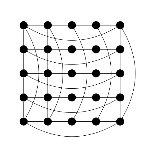
We can consider a system of interacting atoms arranged in a network-like structure (Fig. 1). The state of an atom is defined by its dipole nuclear magnetic moment: a two-valued spin representing the orientation of the magnetic field produced by the atom. Intuitively, neighboring atoms with the same spin value contribute less to the total energy of the system than atoms with different spin values. Systems of this kind evolve preferentially to states with the lowest possible energy. When the temperature of the environment is increased, the system heats, and we can observe a sudden change in a global property of the system, namely loss of magnetization. A theoretical model of such a system of atoms is the Ising model (Ising, 1925; Glauber, 1963).
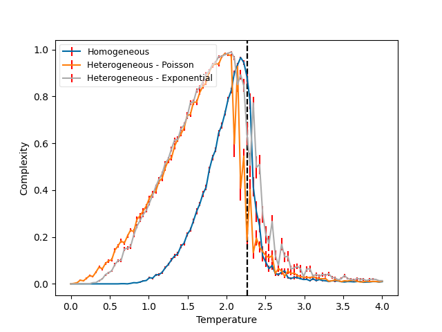
The Ising model is usually homogeneous: all cells have the same temperature, and one explores different properties as the temperature varies. This is a good assumption when all atoms can be considered to behave in a similar way. However, if we are modeling an Ising-like biological system (Hopfield, 1982), then each element might have slightly different properties. In the proposed heterogeneous case, each cell has a temperature taken from a Poisson distribution with a mean equal to the temperature of the homogeneous case (see Sec. 4.1 for details).
Following Lopez-Ruiz et al. (1995), we have proposed a measure of complexity (Fernández et al., 2014) based on Shannon’s information (Shannon, 1948),
| (1) |
where is a positive constant and is the length of the alphabet (for all the cases considered in this paper, ). This measure is equivalent to the Boltzmann-Gibbs entropy. To normalize to , we use
| (2) |
is maximal when the probabilities are homogeneous, i.e. there is the same probability of observing any symbol along a string. is minimal when only one symbol is found in a string (so it has a probability of one, and all the rest have a probability of zero). Chaotic dynamics are characterized by a high , while ordered (static) dynamics are characterized by a low . Inspired by Lopez-Ruiz et al. (1995), we define complexity as the balance between ordered and chaotic dynamics,
| (3) |
where the constant 4 is added to normalize the measure to (Santamaría-Bonfil et al., 2017).
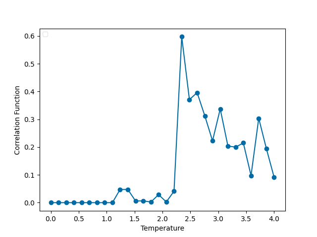
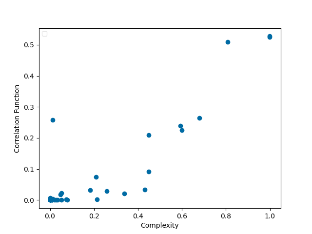
Figure 1 shows the correlation of the Ising model for varying temperature. This is maximal in the phase transition at , i.e. criticality. Figure 1 shows that there is a correspondence between the correlation and the complexity measure in Eq. 3. Figure 1 shows results of average complexity as increases. Complexity is maximal near the phase transition for the homogeneous case. Heterogeneity shifts the expected maximum complexity (that reflects criticality), but it also expands it, in the sense that the area under the curve is broadened. In other words, critical-like dynamics (one can assume arbitrarily complexity values greater than 0.8, just for comparison) are found for a broader range of values.
2.2 Temporal and structural heterogeneity: random Boolean networks
A gene is a part of the genomic sequence that encodes how to produce (synthesise) either a protein or some RNA (gene products). Gene product synthesis is called gene expression. Because not all gene products are synthesised at the same time, the regulation of gene expression is constantly taking place within a cell. In fact, the expression of each gene is regulated (among many things) by the expression of other genes in the genome. This gives rise to an interaction structure known as a genetic regulatory network. Boolean networks are a theoretical model of genetic regulatory networks. In random Boolean networks (RBNs) (Kauffman, 1969, 1993), traditionally there is homogeneous topology and updating. In this case, critical dynamics are found close to a phase transition between ordered and chaotic phases (Derrida and Pomeau, 1986; Luque and Solé, 1997; Wang et al., 2010).
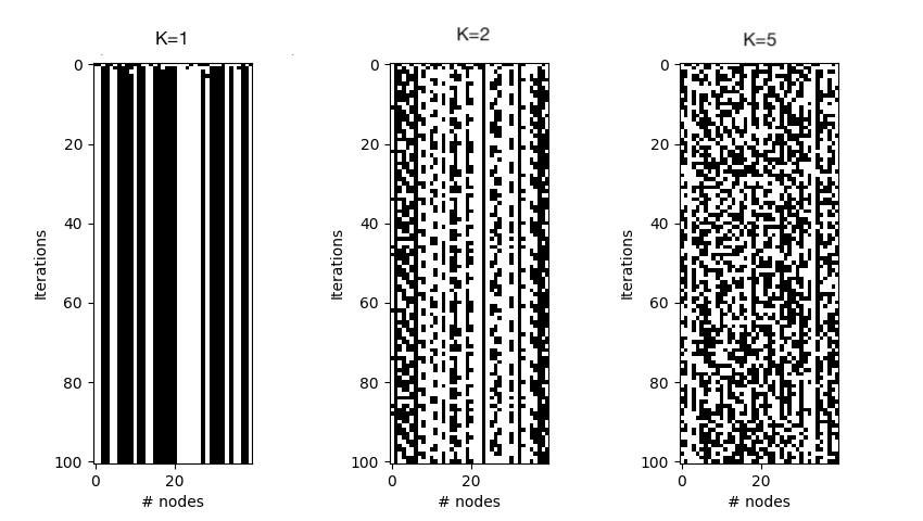
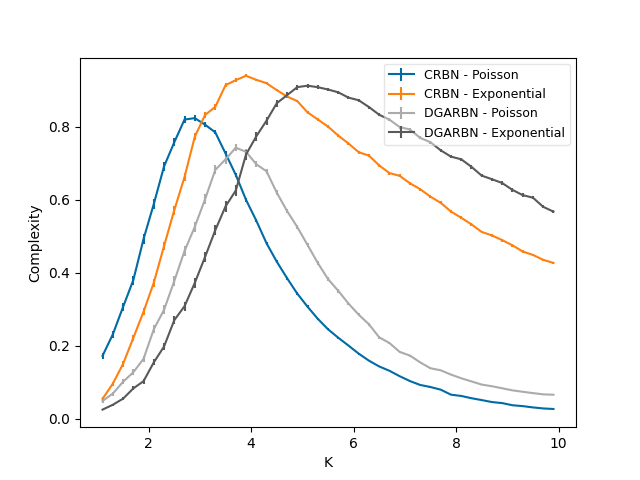
Figure 2 shows an example of the topology of a RBN with seven nodes () and two connections (inputs ) each. Each node has a lookup table where all possible combinations of their inputs are specified (e.g. Figure 2). Using an ensemble approach, for each parameter combination, we randomly generate topologies (structure) and lookup tables (function), and then evaluate them in simulations. Depending on different parameters, the dynamics of RBNs can be classified as ordered, critical (near a phase transition), and chaotic. Figure 2 shows example of these dynamics for different values.
One can have heterogeneous topology in different ways (Oosawa and Savageau, 2002; Aldana, 2003), as genetic regulatory networks are not homogeneous: few genes affect many genes, and many genes affect few genes. Here, we use Poisson and exponential distributions. Strictly speaking, both are heterogeneous, but exponential is more heterogeneous than Poisson, which here we consider as “homogeneous”. The technical reason for using a Poisson distribution is that it allows us to explore non-integer average connectivity in the network.
We can also have heterogeneous updating schemes (Gershenson, 2002), as it can be argued that not all genes in a network “march in step” (Harvey and Bossomaier, 1997). Classical RBNs (CRBNs) have synchronous, homogeneous temporality, while in here we use Deterministic Generalized Asynchronous RBNs (DGARBNs) for heterogeneous temporality. In particular, each node is updated every number of time steps equal to its out-degree, so the more nodes one node affects, the slower it will be updated (see Sec 4.2 for details).
Fig. 2 compares the average complexity as the average connectivity is increased. Structural and temporal homogeneity (CRBN-Poisson) has a classical complexity profile, maximizing near the phase transition ( for the thermodynamical limit, i.e., ). It can be seen that only structural heterogeneity (CRBN-Exponential) extends criticality more than only temporal heterogeneity (DGARBN-Poisson), that basically shifts the curve to the right. Still, having both structural and temporal heterogeneity (DGARBN-Exponential) extends criticality even more than having only structural heterogeneity.
2.3 Arbitrary complexity
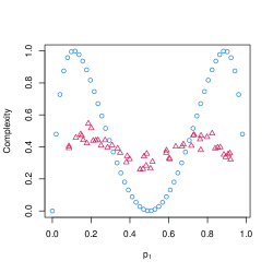
Abstracting the results from the previous subsections, and trying not to depend on any model in particular, we can explore exhaustively the measure of complexity (Eq. 3) in homogeneous and heterogeneous settings, to observe when each case yields a higher average complexity. So we simply vary the probability of having ones in a binary string directly as shown in Figure 3.
In the homogeneous case, we calculate directly the complexity as a function of using Eq. 3, assuming that we are averaging the complexities of several elements with the same . For the heterogeneous case, we generate a collection of probabilities with mean and standard deviation of 0.2 (truncating to zero negative values and to one values greater than one), calculate their complexity, and then average it. Heterogeneity achieves higher complexities for roughly . One might wonder why all heterogenous complexities avoid extreme values, even when heterogeneous RBNs can have complexities close to zero and one. This is because of the standard deviation of the distributions from which the means are generated. Smaller standard deviations yield curves closer to the heterogeneous case.
By assuming that heterogeneity sometimes will be better than homogeneity and vice versa, we can further generalize our results to be independent of any measure or function. If we have homogeneity of a variable , all elements will have the same value for , and thus the mean will be equal to any . Thus, the average of any function will be equal to any . If we have heterogeneity, then the mean will be given by some distribution of different values of , and similarly for .
We can then say that heterogeneity is preferred when the function of the average is greater than the average of the function,
| (4) |
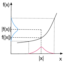
Jensen’s inequality (McShane, 1937) tells us already that heterogeneity will be “better” than homogeneity for concave functions, as illustrated in Figure 3. For more complex functions, their concave parts will benefit from heterogeneity and their convex parts will benefit from homogeneity (as it can be seen for in Figure 3).
For linear functions, it can be shown that there is no difference between homogeneity and heterogeneity, as will always be equal to (see proof in Section 4.3). Thus, it can be concluded that the difference between homogeneity and heterogeneity is relevant only for nonlinear functions.
3 Discussion
There are several recent examples of heterogeneity offering advantages when compared to homogeneous systems in the literature. For example, in public transportation systems, theory tells us that passengers are served optimally (wait at stations for a minimum time) if headways are equal, i.e., homogeneous. However, equal headways are unstable (Gershenson and Pineda, 2009; Chen et al., 2021). Still, adaptive heterogeneous headways can deliver supraoptimal performance through self-organization (Gershenson, 2011; Carreón et al., 2017), due to the slower-is-faster effect (Gershenson and Helbing, 2015): passengers do wait more time at stations, but once they board a vehicle, on average they will reach faster their destination, as the idling required to maintain equal headways is avoided.
There are other examples where heterogeneity promotes synchronization (see Zhang et al. (2021) and references therein). In particular, Zhang et al. (2021) shows that random parameter heterogeneity among oscillators can consistently rescue the system from losing synchrony. In related work, Molnar et al. (2021) finds that heterogeneous generators improve stability in power grids. Recently, Ratnayake et al. (2021) explored complex networks with heterogeneous nodes, observing that these have a greater robustness as compared to networks with homogeneous nodes. In social networks, Zhou et al. (2020) finds that heterogeneity of social status may drive the network evolution towards self-optimization. Also, structural heterogeneity has been shown to favor the evolution of cooperation (Santos et al., 2006, 2008).
These examples suggest that heterogenous networks improve information processing. With heterogeneity, elements can in principle process information differently, potentially increasing the computing power of a heterogeneous system over an homogeneous one with similar characteristics. This is related to Ashby’s law of requisite variety (Ashby, 1956; Gershenson, 2015), which states that an active controller should have at least the same variety (number of states) as the controlled. It is straightforward to see with random Boolean networks that temporal heterogeneity increases the variety of the system: the state space (of size for homogeneous temporality) can explode once we have to include the precise periods and phases of all nodes (in heterogeneous temporality), as different combinations of the temporal substates may lead a transition from the same node substate to different node substates. Also in random Boolean networks, higher implies more possible nets. Even if there are evolutionary pressures for efficiency (smaller networks), if heterogeneity shifts criticality to higher , then it will be easier for an evolutionary search to find critical dynamics in larger spaces.
Shannon’s (1948) information, equivalent to Boltzmann-Gibbs entropy, is maximal when the probability of every symbol or state is the same, i.e. homogeneous. Thus, one can measure heterogeneity as an inverse of entropy (one minus the normalized Shannon’s information) (Fernández et al., 2014). It is clear that maximum heterogeneity (as measured here, it would occur when only one symbol or state has a probability of one and all the rest a probability of zero) has its limitations. Thus, we can assume that there will be an “optimal” balance between minimum and maximum heterogeneities. The precise balance will probably depend on the system, its context, and may even change in time. If we want heterogeneity to take the dynamics towards criticality (or somewhere else), then the precise “optimal” heterogeneity will depend on how far we are from criticality (Gershenson, 2012; Pineda et al., 2019). In this sense, a potential relationship with no-free-lunch theorems (Wolpert and Macready, 1995, 1997) seems an interesting area of further research.
When homogeneous systems are analyzed in terms of their symmetries, heterogeneity is a type of symmetry breaking. Still, in converse symmetry breaking (Nishikawa and Motter, 2016), only heterogeneity leads to stability, i.e. the system symmetry is broken to preserve the state symmetry. This idea can be used to control the stability of complex systems using heterogeneity (Nicolaou et al., 2021). A further avenue of research is the relationship between heterogeneity and Lévy flights (Iñiguez et al., 2022). Lévy flights are heterogeneous, since they consist of many short jumps and few large ones. They offer a balance between exploration and exploitation, and seem advantageous for foraging (Ramos-Fernández et al., 2004), preventing extinctions (Dannemann et al., 2018), and search algorithms (Martínez-Arévalo et al., 2020). Another interesting relationship to study is the one between heterogeneity and non-reciprocal systems (Fruchart et al., 2021).
Network science (Albert and Barabasi, 2002; Newman, 2003; Barabási, 2016) has demonstrated the relevance of structural heterogeneity. This should be complemented with a systematic exploration of temporal (Barabási, 2005) and other types of heterogeneity. For example, it would be interesting to study heterogeneous adaptive (Gross and Sayama, 2009) and temporal (Holme and Saramäki, 2012; Holme, 2015) networks, where each node has a different speed for its dynamics. Temporal heterogeneity enables a system to match the requisite variety of their environment at different timescales. If systems can adapt at the scales at which their environments change, then they will better do so if they have a variety of timescales, i.e., heterogeneous temporality. Recently, Sormunen et al. (2022) have shown that adaptive networks have critical manifolds that can be navigated as parameters change. In other words, criticality is not restricted to a single value, but can be associated to a manifold in a multidimensional system.
Further research is required to better understand the role of heterogeneity in the criticality of complex systems. The present work is limited and many open questions remain. We encourage the reader to experiment with a heterogeneous version of their favorite homogeneous complex system model, be it structural, temporal, or other type of heterogeneity. We could learn more from heterogeneous models of collective motion, opinion formation, financial markets, urban growth, and more. This could contribute to a broader understanding of heterogeneity and its relationship with criticality.
4 Methods
A graph consists of a set of vertices and a set of edges , where an edge is an unordered pair of distinct vertices of . We write to denote that is an edge and in this case we say that and are adjacent. If is a graph with vertex set and edge set , we say that is a subgraph of . A graph is said to be connected if for every pair of distinct vertices and , there is a finite sequence of distinct vertices such that , , and for each . A connected component of is a connected subgraph of . A graph is said to be finite just in case its vertex set is finite. A graph is called -regular if every vertex is adjacent to exactly distinct vertices.
A directed graph consists of a set of elements called the nodes of and a set of ordered pairs of nodes called the arcs of . We use the symbol to represent the arc . If is in the arc set of , then we say that is an incoming neighbour (or in-neighbour) of , and also that is a outgoing neighbour (or out-neighbour) of . We say that is -in regular () if every node has exactly in-neighbours: for every node there are distinct nodes , such that for . In other words, is -in regular just in case the set of in-neighbours of any node has exactly elements, all distinct, and possibly including itself. The out-degree of a node is the number of nodes such that the arc is in the arc set of . Thus the out-degree of is the number of out-neighbours of . Similarly, the in-degree of a node is the number of nodes such that . Thus the in-degree of is the number of in-neighbours of .
4.1 The Ising model with individual temperatures
It is quite common to study the Ising model on a finite, connected -regular graph where the number of edges is twice the number of vertices. This graph is usually introduced as a finite lattice of two-dimensional points on the surface of a three-dimensional torus. An example of such a graph with vertices and edges is shown in Figure 1.
4.1.1 The Ising model
We start with a finite graph . We identify the vertex set of with a system of interacting atoms. Each vertex is assigned a spin which can take the value or . The energy of a configuration of spins is
The energy increases with the number of pairs of adjacent vertices having different spins. The Ising model is a way to assign probabilities to the system configurations. The probability of a configuration is proportional to , where is a variable inversely proportional to the temperature.
More precisely, the Ising model with inverse temperature is the probability measure on the set of configurations defined by
where is a normalizing constant. This constant can be computed explicitly as
where denotes the cardinality of a finite set , and the number of connected components of the (spanning) subgraph of . Then
where and so, for any configuration , we have that
As the temperature increases (and hence ), converges to the uniform measure over the space of configurations. When the temperature decreases, increases, and assigns greater probability to configurations that have a large number of pairs of adjacent vertices with the same spin.
4.1.2 Simulation
Most simulations of the Ising model use either the Glauber dynamics or the Metropolis algorithm for constructing a Markov chain with stationary measure . Here we only describe the Metropolis chain for the Ising model.
Given two configurations , let denote the probability that the Metropolis chain for the Ising model moves from to . For every , we write to denote the configuration obtained from by flipping the sign of the value that assigns to and leaving all the other spins the same. In other words, is the unique configuration which agrees everywhere with except for the spin assigned to vertex : for every , if and if . We let the transition probabilities to be positive just in case or for some . In the latter case, the Metropolis chain moves from to with probability
where denotes the minimum of the quantities and . The probability that the chain stays at the same configuration is then
A key property about these transition probabilities is that they only depend on the ratios . Therefore, to simulate the Metropolis chain it is not necessary to compute the normalizing constant of the Ising measure .
To summarize, we have constructed a transition matrix that defines a reversible Markov chain with stationary measure .
Proposition 1.
The Metropolis chain for the Ising model has stationary measure .
Proof.
It is sufficient to prove that the probability measure and the transition matrix satisfy the detailed balance equations
| (5) |
for all . To show this, it suffices to verify that the equation (5) holds when for some . After cancellation of and distributing and accordingly, it suffices to check
or equivalently
which is obvious. ∎
4.1.3 Individual temperatures
In the previous section, we described how to construct a transition matrix that defines a reversible Markov chain with stationary measure . Starting at a configuration , the probability that the chain moves to a new configuration for any , is given by
where
Thus, the transition probability from to of the Metropolis chain for the Ising model with parameter is determined by the quantity
We now turn to study a situation where each vertex has its own parameter . In other word, we shall describe a Markov chain that moves from to with probability depending on
where is a individual (possibly distinct) parameter for each . More precisely, the probability that the new chain moves from to is defined as
The probability that the chain stays at the same configuration is
Hence, all the configurations that differ from in at least two vertices are not reachable from . That is to say, if and only if for any .
Definition 1 (Ising measure with individual temperatures).
Let be a finite, connected graph and a collection of non-negative real numbers. The probability measure on is defined by
where is a normalizing constant.
Remark 1.
We can think of as an heterogenous Ising model as opposed to the homogeneous version defined in Section 4.1.1 by
Remark 2.
It is cleat that the probability measure is a stationary measure of the Markov chain defined by the transition matrix just in case we have for all . In other words, if and only if the individual parameters in the definition of are all equal to the single parameter of the homogeneous Ising model.
Proposition 2.
The probability measure is the stationary measure of the Markov chain defined by the transition matrix .
Proof.
In order to satisfy the detailed balanced equations
we must have
for all and , because
Now, if then , and hence , so
Otherwise, if then , and so , hence
In both cases, we arrive at the conclusion that in order for to be the stationary measure of the chain defined by , we must have
| (6) |
for every and .
Now we proceed to prove that equation (6) holds. After cancellation of and using properties of the exponential function, it suffices to check
By inspection,
Therefore, the probability measure and the transition matrix satisfy the detailed balance equations and the result follows. ∎
4.2 Random Boolean networks
4.2.1 Homogeneous random Boolean networks
Let be a directed graph. We identify the nodes of with the genes in a gene regulatory network. Suppose is a -in regular directed graph. Figure 2 is an example of a -in regular digraph with nodes, i.e. .
A family of functions is called a Boolean network on . Figure 2 is an example of a Boolean network on a graph with nodes, and with the parameter of “connectivity” equal to . A Boolean network is called random if the assignment is made at random by sampling independently and uniformly from the set of all the Boolean functions with inputs. A function , is called a state of the random Boolean network on . The value is called the state of . The updating function of a state is the function defined as
For every , we have a sequence of states such that each state is the updating function of the previous state in the sequence: , and so on. The sequence of states is called the time series of .
4.2.2 Heterogeneous random Boolean networks
The description given in 4.2.1 corresponds to the case where the structure and the updating scheme of the random Boolean network are homogeneous. Here we describe the two versions of heterogeneous random Boolean networks that were used in the simulations. The first of these heterogeneous descriptions is structural, while the second gives rise to some sort of asynchronous dynamics.
The definition of Boolean network above makes the assumption that every node in the directed graph has the same in-degree. Now we consider Boolean networks over arbitrary (not necessarily -in regular, directed) graphs. A generalized Boolean network on a directed graph consists of a family of functions with the in-degree . Thus a heterogeneous random Boolean network is a generalized Boolean network chosen uniformly at random.
For talking about temporal heterogeneity we need to introduce asynchronous updating schemes (Gershenson, 2002). The heterogeneous updating function of a state of a random heterogeneous Boolean network on is the function , defined by
where is called the discrete time-step, and is the out-degree of : there are nodes all distinct, such that for .
4.3 Linear functions
Here we observe that for linear functions, there is no difference between homogeneity and heterogeneity. Indeed a function with is called linear if for all and all , we have
For , it can be shown, by induction on the number of points , that
Thus, in the context of linear functions, average value (heterogeneity) is the same as value of the average (homogeneity).
Acknowledgments
O. Z. acknowledges support from CONACyT-SNI (Grant No. 620178). G.I. acknowledges support from AFOSR (Grant No. FA8655-20-1-7020), project EU H2020 Humane AI-net (Grant No. 952026), and CHIST-ERA project SAI (Grant No. FWF I 5205-N). C.G. acknowledges support from UNAM-PAPIIT (IN107919, IV100120, IN105122) and from the PASPA program from UNAM-DGAPA.
Author contributions
All authors conceived and designed the study. F.S.P., O.Z., and O.K.P. performed numerical simulations and derived mathematical results. All authors wrote the paper.
Competing interest statement
All authors declare no competing interest.
References
- Adami (1995) Adami, C. (1995). Self-organized criticality in living systems. Phys. Lett. A 203: 29–32. URL http://arxiv.org/abs/adap-org/9401001.
- Albert and Barabasi (2002) Albert, R. and Barabasi, A.-L. (2002). Statistical mechanics of complex networks. Reviews of Modern Physics 74: 47–97.
- Aldana (2003) Aldana, M. (2003). Boolean dynamics of networks with scale-free topology. Physica D 185 (1): 45–66. URL http://dx.doi.org/10.1016/S0167-2789(03)00174-X.
- Anderson (1972) Anderson, P. W. (1972). More is different. Science 177: 393–396.
- Ashby (1956) Ashby, W. R. (1956). An Introduction to Cybernetics. Chapman & Hall, London. URL http://pcp.vub.ac.be/ASHBBOOK.html.
- Bak et al. (1987) Bak, P., Tang, C., and Wiesenfeld, K. (1987). Self-organized criticality: An explanation of the 1/f noise. Phys. Rev. Lett. 59 (4) (July): 381–384. URL http://dx.doi.org/10.1103/PhysRevLett.59.381.
- Balleza et al. (2008) Balleza, E., Alvarez-Buylla, E. R., Chaos, A., Kauffman, S., Shmulevich, I., and Aldana, M. (2008). Critical dynamics in genetic regulatory networks: Examples from four kingdoms. PLoS ONE 3 (6) (06): e2456. URL http://dx.plos.org/10.1371%2Fjournal.pone.0002456.
- Barabási (2005) Barabási, A.-L. (2005). The origin of bursts and heavy tails in human dynamics. Nature 435 (7039): 207–211. URL https://doi.org/10.1038/nature03459.
- Barabási (2016) Barabási, A.-L. (2016). Network Science. Cambridge University Press, Cambridge, UK. URL http://barabasi.com/networksciencebook/.
- Beggs (2008) Beggs, J. M. (2008). The criticality hypothesis: how local cortical networks might optimize information processing. Philosophical Transactions of the Royal Society A: Mathematical, Physical and Engineering Sciences 366 (1864): 329–343. URL https://royalsocietypublishing.org/doi/abs/10.1098/rsta.2007.2092.
- Carreón et al. (2017) Carreón, G., Gershenson, C., and Pineda, L. A. (2017). Improving public transportation systems with self-organization: A headway-based model and regulation of passenger alighting and boarding. PLOS ONE 12 (12) (12): 1–20. URL https://doi.org/10.1371/journal.pone.0190100.
- Chen et al. (2021) Chen, T., Quek, W. L., Chung, N. N., Saw, V.-L., and Chew, L. Y. (2021). Analysis and simulation of intervention strategies against bus bunching by means of an empirical agent-based model. Complexity 2021: 2606191. URL https://doi.org/10.1155/2021/2606191.
- Chialvo (2010) Chialvo, D. R. (2010). Emergent complex neural dynamics. Nature Physics 6 (10): 744–750. URL https://doi.org/10.1038/nphys1803.
- Chowdhury et al. (2000) Chowdhury, D., Santen, L., and Schadschneider, A. (2000). Statistical physics of vehicular traffic and some related systems. Physics Reports 329 (4-6): 199 – 329. URL http://dx.doi.org/10.1016/S0370-1573(99)00117-9.
- Christensen and Moloney (2005) Christensen, K. and Moloney, N. R. (2005). Complexity and criticality. World Scientific, Singapore.
- Cocho et al. (2015) Cocho, G., Flores, J., Gershenson, C., Pineda, C., and Sánchez, S. (2015). Rank diversity of languages: Generic behavior in computational linguistics. PLoS ONE 10 (4) (04): e0121898. URL http://dx.doi.org/10.1371%2Fjournal.pone.0121898.
- Dannemann et al. (2018) Dannemann, T., Boyer, D., and Miramontes, O. (2018). Lévy flight movements prevent extinctions and maximize population abundances in fragile lotka–volterra systems. Proceedings of the National Academy of Sciences 115 (15): 3794–3799. URL https://www.pnas.org/content/115/15/3794.
- Derrida and Pomeau (1986) Derrida, B. and Pomeau, Y. (1986). Random networks of automata: A simple annealed approximation. Europhys. Lett. 1 (2): 45–49.
- Fernández et al. (2014) Fernández, N., Maldonado, C., and Gershenson, C. (2014). Information measures of complexity, emergence, self-organization, homeostasis, and autopoiesis. In Guided Self-Organization: Inception, M. Prokopenko, (Ed.). Emergence, Complexity and Computation, vol. 9. Springer, Berlin Heidelberg, 19–51. URL http://arxiv.org/abs/1304.1842.
- Fruchart et al. (2021) Fruchart, M., Hanai, R., Littlewood, P. B., and Vitelli, V. (2021). Non-reciprocal phase transitions. Nature 592 (7854): 363–369. URL https://doi.org/10.1038/s41586-021-03375-9.
- Gershenson (2002) Gershenson, C. (2002). Classification of random Boolean networks. In Artificial Life VIII: Proceedings of the Eight International Conference on Artificial Life, R. K. Standish, M. A. Bedau, and H. A. Abbass, (Eds.). MIT Press, Cambridge, MA, USA, pp. 1–8. URL http://arxiv.org/abs/cs/0208001.
- Gershenson (2011) Gershenson, C. (2011). Self-organization leads to supraoptimal performance in public transportation systems. PLoS ONE 6 (6): e21469. URL http://dx.doi.org/10.1371/journal.pone.0021469.
- Gershenson (2012) Gershenson, C. (2012). Guiding the self-organization of random Boolean networks. Theory in Biosciences 131 (3) (September): 181–191. URL http://arxiv.org/abs/1005.5733.
- Gershenson (2015) Gershenson, C. (2015). Requisite variety, autopoiesis, and self-organization. Kybernetes 44 (6–7): 866–873.
- Gershenson and Helbing (2015) Gershenson, C. and Helbing, D. (2015). When slower is faster. Complexity 21 (2): 9–15. URL http://dx.doi.org/10.1002/cplx.21736.
- Gershenson and Pineda (2009) Gershenson, C. and Pineda, L. A. (2009). Why does public transport not arrive on time? The pervasiveness of equal headway instability. PLoS ONE 4 (10): e7292. URL http://dx.doi.org/10.1371/journal.pone.0007292.
- Glauber (1963) Glauber, R. J. (1963). Time-dependent statistics of the Ising model. Journal of Mathematical Physics 4 (2): 294–307. URL http://dx.doi.org/10.1063/1.1703954.
- Gross and Sayama (2009) Gross, T. and Sayama, H., Eds. (2009). Adaptive networks: Theory, Models and Applications. Understanding Complex Systems. Springer, Berlin Heidelberg. URL http://dx.doi.org/10.1007/978-3-642-01284-6.
- Harvey and Bossomaier (1997) Harvey, I. and Bossomaier, T. (1997). Time out of joint: Attractors in asynchronous random Boolean networks. In Proceedings of the Fourth European Conference on Artificial Life (ECAL97), P. Husbands and I. Harvey, (Eds.). MIT Press, pp. 67–75. URL http://tinyurl.com/yxrxbp.
- Helbing (2001) Helbing, D. (2001). Traffic and related self-driven many-particle systems. Reviews of modern physics 73 (4): 1067.
- Hesse and Gross (2014) Hesse, J. and Gross, T. (2014). Self-organized criticality as a fundamental property of neural systems. Frontiers in systems neuroscience 8: 166.
- Hidalgo et al. (2016) Hidalgo, J., Grilli, J., Suweis, S., Maritan, A., and Muñoz, M. A. (2016). Cooperation, competition and the emergence of criticality in communities of adaptive systems. Journal of Statistical Mechanics: Theory and Experiment 2016 (3) (mar): 033203. URL https://doi.org/10.1088/1742-5468/2016/03/033203.
- Holme (2015) Holme, P. (2015). Modern temporal network theory: a colloquium. Eur. Phys. J. B 88 (9): 1–30.
- Holme and Saramäki (2012) Holme, P. and Saramäki, J. (2012). Temporal networks. Physics Reports 519 (3): 97 – 125. URL http://arxiv.org/abs/1108.1780.
- Hopfield (1982) Hopfield, J. J. (1982). Neural networks and physical systems with emergent collective computational abilities. Proceedings of the National Academy of Sciences 79 (8): 2554–2558. URL https://www.pnas.org/doi/abs/10.1073/pnas.79.8.2554.
- Iñiguez et al. (2022) Iñiguez, G., Pineda, C., Gershenson, C., and Barabási, A.-L. (2022). Dynamics of ranking. Nature Communications 13 (1): 1646. URL https://doi.org/10.1038/s41467-022-29256-x.
- Ising (1925) Ising, E. (1925). Beitrag zur theorie des ferromagnetismus. Zeitschrift für Physik 31 (1): 253–258.
- Kauffman (1969) Kauffman, S. A. (1969). Metabolic stability and epigenesis in randomly constructed genetic nets. Journal of Theoretical Biology 22: 437–467.
- Kauffman (1993) Kauffman, S. A. (1993). The Origins of Order. Oxford University Press, Oxford, UK.
- Langton (1990) Langton, C. G. (1990). Computation at the edge of chaos: Phase transitions and emergent computation. Physica D 42: 12–37.
- Lloyd (2001) Lloyd, S. (2001). Measures of complexity: a non-exhaustive list. Department of Mechanical Engineering, Massachusetts Institute of Technology. URL http://web.mit.edu/esd.83/www/notebook/Complexity.PDF.
- Lopez-Ruiz et al. (1995) Lopez-Ruiz, R., Mancini, H. L., and Calbet, X. (1995). A statistical measure of complexity. Physics Letters A 209 (5-6): 321–326. URL http://dx.doi.org/10.1016/0375-9601(95)00867-5.
- Luque and Solé (1997) Luque, B. and Solé, R. V. (1997). Phase transitions in random networks: Simple analytic determination of critical points. Physical Review E 55 (1): 257–260. URL http://tinyurl.com/y8pk9y.
- Martínez-Arévalo et al. (2020) Martínez-Arévalo, Y. I., Rodríguez-Vazquez, K., and Gershenson, C. (2020). Temporal heterogeneity improves speed and convergence in genetic algorithms. arXiv:2203.13194.
- McShane (1937) McShane, E. J. (1937). Jensen’s inequality. Bulletin of the American Mathematical Society 43 (8): 521–527.
- Molnar et al. (2021) Molnar, F., Nishikawa, T., and Motter, A. E. (2021). Asymmetry underlies stability in power grids. Nature Communications 12 (1): 1457. URL https://doi.org/10.1038/s41467-021-21290-5.
- Mora and Bialek (2011) Mora, T. and Bialek, W. (2011). Are biological systems poised at criticality? Journal of Statistical Physics 144 (2): 268–302. URL https://doi.org/10.1007/s10955-011-0229-4.
- Morales et al. (2018) Morales, J. A., Colman, E., Sánchez, S., Sánchez-Puig, F., Pineda, C., Iñiguez, G., Cocho, G., Flores, J., and Gershenson, C. (2018). Rank dynamics of word usage at multiple scales. Frontiers in Physics 6: 45. URL https://www.frontiersin.org/article/10.3389/fphy.2018.00045.
- Morales et al. (2016) Morales, J. A., Sánchez, S., Flores, J., Pineda, C., Gershenson, C., Cocho, G., Zizumbo, J., Rodríguez, R. F., and Iñiguez, G. (2016). Generic temporal features of performance rankings in sports and games. EPJ Data Science 5 (1): 33. URL http://dx.doi.org/10.1140/epjds/s13688-016-0096-y.
- Muñoz (2018) Muñoz, M. A. (2018). Colloquium: Criticality and dynamical scaling in living systems. Rev. Mod. Phys. 90: 031001. URL https://link.aps.org/doi/10.1103/RevModPhys.90.031001.
- Newman (2003) Newman, M. E. J. (2003). The structure and function of complex networks. SIAM Review 45: 167–256. URL http://arxiv.org/abs/cond-mat/0303516.
- Nicolaou et al. (2021) Nicolaou, Z. G., Case, D. J., Wee, E. B. v. d., Driscoll, M. M., and Motter, A. E. (2021). Heterogeneity-stabilized homogeneous states in driven media. Nature Communications 12 (1): 4486. URL https://doi.org/10.1038/s41467-021-24459-0.
- Nishikawa and Motter (2016) Nishikawa, T. and Motter, A. E. (2016). Symmetric states requiring system asymmetry. Phys. Rev. Lett. 117: 114101. URL https://link.aps.org/doi/10.1103/PhysRevLett.117.114101.
- Oosawa and Savageau (2002) Oosawa, C. and Savageau, M. A. (2002). Effects of alternative connectivity on behavior of randomly constructed Boolean networks. Physica D 170: 143–161.
- Pineda et al. (2019) Pineda, O. K., Kim, H., and Gershenson, C. (2019). A novel antifragility measure based on satisfaction and its application to random and biological Boolean networks. Complexity 2019: 10. URL https://doi.org/10.1155/2019/3728621.
- Prokopenko et al. (2011) Prokopenko, M., Lizier, J. T., Obst, O., and Wang, X. R. (2011). Relating Fisher information to order parameters. Phys. Rev. E 84: 041116. URL http://dx.doi.org/10.1103/PhysRevE.84.041116.
- Ramos-Fernández et al. (2004) Ramos-Fernández, G., Mateos, J., Miramontes, O., Cocho, G., Larralde, H., and Ayala-Orozco, B. (2004). Lévy walk patterns in the foraging movements of spider monkeys (Ateles geoffroyi). Behavioral Ecology and Sociobiology 55 (3): 223–230. URL https://doi.org/10.1007/s00265-003-0700-6.
- Ratnayake et al. (2021) Ratnayake, P., Weragoda, S., Wansapura, J., Kasthurirathna, D., and Piraveenan, M. (2021). Quantifying the robustness of complex networks with heterogeneous nodes. Mathematics 9 (21). URL https://www.mdpi.com/2227-7390/9/21/2769.
- Roli et al. (2018) Roli, A., Villani, M., Filisetti, A., and Serra, R. (2018). Dynamical criticality: Overview and open questions. Journal of Systems Science and Complexity 31 (3): 647–663. URL https://doi.org/10.1007/s11424-017-6117-5.
- Santamaría-Bonfil et al. (2016) Santamaría-Bonfil, G., Fernández, N., and Gershenson, C. (2016). Measuring the complexity of continuous distributions. Entropy 18 (3): 72. URL http://www.mdpi.com/1099-4300/18/3/72.
- Santamaría-Bonfil et al. (2017) Santamaría-Bonfil, G., Gershenson, C., and Fernández, N. (2017). A package for measuring emergence, self-organization, and complexity based on Shannon entropy. Frontiers in Robotics and AI 4: 10. URL http://journal.frontiersin.org/article/10.3389/frobt.2017.00010.
- Santos et al. (2006) Santos, F. C., Pacheco, J. M., and Lenaerts, T. (2006). Evolutionary dynamics of social dilemmas in structured heterogeneous populations. Proc. Natl. Acad. Sci. USA 103: 3490–3494. URL http://www.pnas.org/content/103/9/3490.long.
- Santos et al. (2008) Santos, F. C., Santos, M. D., and Pacheco, J. M. (2008). Social diversity promotes the emergence of cooperation in public goods games. Nature 454 (7201): 213–216. URL http://www.nature.com/nature/journal/v454/n7201/full/nature06940.html.
- Shannon (1948) Shannon, C. E. (1948). A mathematical theory of communication. Bell System Technical Journal 27 (3 and 4) (July and October): 379–423 and 623–656. URL http://dx.doi.org/10.1002/j.1538-7305.1948.tb01338.x.
- Shmulevich et al. (2005) Shmulevich, I., Kauffman, S. A., and Aldana, M. (2005). Eukaryotic cells are dynamically ordered or critical but not chaotic. Proceedings of the National Academy of Sciences 102 (38): 13439–13444. URL https://www.pnas.org/doi/abs/10.1073/pnas.0506771102.
- Sormunen et al. (2022) Sormunen, S., Gross, T., and Saramäki, J. (2022). Critical drift in a neuro-inspired adaptive network. arXiv:2206.10315v1.
- Stanley (1987) Stanley, H. E. (1987). Introduction to phase transitions and critical phenomena. Oxford University Press, Oxford, UK.
- Torres-Sosa et al. (2012) Torres-Sosa, C., Huang, S., and Aldana, M. (2012). Criticality is an emergent property of genetic networks that exhibit evolvability. PLoS Comput Biol 8 (9) (09): e1002669. URL http://dx.doi.org/10.1371%2Fjournal.pcbi.1002669.
- Vicsek and Zafeiris (2012) Vicsek, T. and Zafeiris, A. (2012). Collective motion. Physics Reports 517: 71–140. URL http://dx.doi.org/10.1016/j.physrep.2012.03.004.
- Vidiella et al. (2020) Vidiella, B., Guillamon, A., Sardanyés, J., Maull, V., Conde-Pueyo, N., and Solé, R. (2020). Engineering self-organized criticality in living cells. bioRxiv 2020.11.16.385385. URL https://www.biorxiv.org/content/early/2020/11/17/2020.11.16.385385.
- Wang et al. (2011) Wang, X., Lizier, J., and Prokopenko, M. (2011). Fisher information at the edge of chaos in random Boolean networks. Artificial Life 17 (4): 315–329. Special Issue on Complex Networks. URL http://dx.doi.org/10.1162/artl_a_00041.
- Wang et al. (2010) Wang, X. R., Lizier, J., and Prokopenko, M. (2010). A Fisher information study of phase transitions in random Boolean networks. In Artificial Life XII Proceedings of the Twelfth International Conference on the Synthesis and Simulation of Living Systems, H. Fellermann, M. Dörr, M. M. Hanczyc, L. L. Laursen, S. Maurer, D. Merkle, P.-A. Monnard, K. Sty, and S. Rasmussen, (Eds.). MIT Press, Odense, Denmark, 305–312. URL http://tinyurl.com/37qxgtn.
- Wolpert and Macready (1995) Wolpert, D. H. and Macready, W. G. (1995). No free lunch theorems for search. Tech. Rep. SFI-WP-95-02-010, Santa Fe Institute. URL http://tinyurl.com/yz274ej.
- Wolpert and Macready (1997) Wolpert, D. H. and Macready, W. G. (1997). No Free Lunch Theorems for Optimization. IEEE Transactions on Evolutionary Computation 1 (1): 67–82.
- Zhang et al. (2021) Zhang, Y., Ocampo-Espindola, J. L., Kiss, I. Z., and Motter, A. E. (2021). Random heterogeneity outperforms design in network synchronization. Proceedings of the National Academy of Sciences 118 (21). URL https://www.pnas.org/content/118/21/e2024299118.
- Zhou et al. (2020) Zhou, B., Lu, X., and Holme, P. (2020). Universal evolution patterns of degree assortativity in social networks. Social Networks 63: 47–55. URL https://www.sciencedirect.com/science/article/pii/S0378873320300253.