Supplemental Material for “Topological spin excitations in non-Hermitian spin chains with a generalized kernel polynomial algorithm”

I Details of the NHKPM method

We derived in the main text that the spectral function

$$f(\omega)=\langle\psi_{\text{L}}|\delta^{2}(\omega-H)|\psi_{\text{R}}\rangle$$ (S1)

can be computed with

$$f(\omega)=\frac{1}{\pi}\partial_{\omega^{*}}G(E=0)$$ (S2)

where

$$G(E)=\langle\text{L}|(E-\mathcal{H})^{-1}|\text{R}\rangle$$ (S3)

is an entry of the Green’s function of the Hermitrized Hamiltonian $\mathcal{H}$ (Eq. (6) in the main text) with

$$|\text{L}\rangle=\left(\begin{array}[]{c}0\\ |\psi_{\text{L}}\rangle\end{array}\right),|\text{R}\rangle=\left(\begin{array}[]{c}|\psi_{\text{R}}\rangle\\ 0\end{array}\right).$$ (S8)

Since $G(E)$ is a function of a single variable, we can apply KPM to compute $G(E)$, let

$$G(E)=B(E)-iA(E),$$ (S9)

where $A(E)=\langle\text{L}|\delta(E-\mathcal{H})|\text{R}\rangle$ and $B(E)$ is its Hilbert transform:

$$B(E)=\frac{1}{\pi}\mathcal{P}\int_{-\infty}^{\infty}\text{d}E^{\prime}\frac{A(E^{\prime})}{E-E^{\prime}},$$ (S10)

where $\mathcal{P}$ denotes the Cauchy principal value. Performing a scaling on $\mathcal{H}$: $\mathcal{H}\to\mathcal{H}/\Delta$ such that its spectrum lies in $(-1,1)$, we can perform a Chebyshev expansion on $A(E)$:

$$A(E)=\frac{1}{\pi\sqrt{1-E^{2}}}\left(\mu_{0}+2\sum_{n=1}^{\infty}\mu_{n}T_{n}(E)\right),$$ (S11)

where

$$\mu_{n}=\int_{-1}^{1}\text{d}EA(E)T_{n}(E)=\langle\text{L}|T_{n}(\mathcal{H})|\text{R}\rangle,$$ (S12)

and $T_{n}(x)=\cos(n\arccos{x})$ satisfying the following recursion relation:

$$\begin{aligned} T_{0}(x)=1,T_{1}(x)=x,\\ T_{n+1}(x)=2xT_{n}(x)-T_{n-1}(x).\end{aligned}$$ (S13)

Using

$$\mathcal{P}\int_{-1}^{1}\frac{T_{n}(y)\text{d}y}{(y-x)\sqrt{1-y^{2}}}=\pi U_{n-1}(x),$$ (S14)

together with Eqs. (S10) and (S11), we have

$$B(E)=\frac{2}{\pi}\sum_{n=1}^{\infty}\mu_{n}U_{n-1}(E)$$ (S15)

where $U_{n}(x)=\sin[(n+1)\arccos{x}]/\sin[\arccos{x}]$. Combining Eqs. (S9),(S11) and (S15), we have

$$G(E=0)=\frac{2}{\pi}\sum_{n=1}^{\infty}(-1)^{n+1}\mu_{2n-1},$$ (S16)

which can be computed by noting that $\mu_{n}=0$ for even $n$ and $T_{n}(0)=U_{n}(0)=0$ for odd $n$. Combining Eq. (S2), Eq. (S12) and Eq. (S16), we have Eq. (8) in the main text:

$$f(\omega)=\frac{2}{\pi^{2}}\sum_{n=1}^{\infty}(-1)^{n+1}\langle\text{L}|\partial_{\omega^{*}}T_{2n-1}(\mathcal{H})|\text{R}\rangle,$$ (S17)

with the recursion relation

$$\begin{aligned} \partial_{\omega^{*}}T_{n+1}(\mathcal{H})=&2\left(\begin{array}[]{cc}&0\\ 1&\end{array}\right)T_{n}(\mathcal{H})\\ &+2\mathcal{H}\partial_{\omega^{*}}T_{n}(\mathcal{H})-\partial_{\omega^{*}}T_{n-1}(\mathcal{H}).\end{aligned}$$ (S18)

We now elaborate on the numerical details in the computation of $f(\omega)$. Let

$$|A_{n}\rangle=T_{n}(\mathcal{H})|\text{R}\rangle$$ (S19)

and

$$|\Psi_{n}\rangle=\partial_{\omega^{*}}T_{n}(\mathcal{H})|\text{R}\rangle.$$ (S20)

We can verify that

$$\begin{aligned} |A_{0}\rangle=\left(\begin{array}[]{c}|\psi_{\text{R}}\rangle\\ 0\end{array}\right)&,|A_{1}\rangle=\left(\begin{array}[]{c}0\\ (\omega^{*}-H^{\dagger})|\psi_{\text{R}}\rangle\end{array}\right)\\ |\Psi_{0}\rangle=\left(\begin{array}[]{c}0\\ 0\end{array}\right)&,|\Psi_{1}\rangle=\left(\begin{array}[]{c}0\\ |\psi_{\text{R}}\rangle\end{array}\right)\end{aligned}$$ (S21)

with recursion relation

$$\begin{aligned} |A_{n+1}\rangle&=2\mathcal{H}|A_{n}\rangle-|A_{n-1}\rangle\\ |\Psi_{n+1}\rangle&=2\left(\begin{array}[]{cc}&0\\ 1&\end{array}\right)|A_{n}\rangle+2\mathcal{H}|\Psi_{n}\rangle-|\Psi_{n-1}\rangle.\end{aligned}$$ (S22)

Let

$$\begin{aligned} |A_{2n}\rangle=\left(\begin{array}[]{c}|\alpha_{2n}\rangle\\ 0\end{array}\right)&,|A_{2n+1}\rangle=\left(\begin{array}[]{c}0\\ |\alpha_{2n+1}\rangle\end{array}\right)\\ |\Psi_{2n}\rangle=\left(\begin{array}[]{c}|\psi_{2n}\rangle\\ 0\end{array}\right)&,|\Psi_{2n+1}\rangle=\left(\begin{array}[]{c}0\\ |\psi_{2n+1}\rangle\end{array}\right)\end{aligned}$$ (S23)

where $n\in\mathbb{Z}$ and $n\geq 0$. We thus arrive at the following recursion relation

$$\begin{aligned} |\alpha_{2n}\rangle&=2(\omega-H)|\alpha_{2n-1}\rangle-|\alpha_{2n-2}\rangle\\ |\alpha_{2n+1}\rangle&=2(\omega^{*}-H^{\dagger})|\alpha_{2n}\rangle-|\alpha_{2n-1}\rangle\\ |\psi_{2n}\rangle&=2(\omega-H)|\psi_{2n-1}\rangle-|\psi_{2n-2}\rangle\\ |\psi_{2n+1}\rangle&=2|\alpha_{2n}\rangle+2(\omega^{*}-H^{\dagger})|\psi_{2n}\rangle-|\psi_{2n-1}\rangle\end{aligned}$$ (S24)

with

$$\begin{aligned} |\alpha_{0}\rangle=|\psi_{\text{R}}\rangle&,|\alpha_{1}\rangle=(\omega^{*}-H^{\dagger})|\psi_{\text{R}}\rangle\\ |\psi_{0}\rangle=0&,|\psi_{1}\rangle=|\psi_{\text{R}}\rangle,\end{aligned}$$ (S25)

and Eq.(S17) becomes

$$f(\omega)=\frac{2}{\pi^{2}}\sum_{n=1}^{\infty}(-1)^{n+1}\langle\psi_{L}|\psi_{2n-1}\rangle.$$ (S26)

In practice, we do a truncation of Eq. (S26) to order $N$:

$$f_{\text{KPM}}(\omega)=\frac{2}{\pi^{2}}\sum_{n=1}^{N}(-1)^{n+1}g^{2N}_{2n-1}\langle\psi_{L}|\psi_{2n-1}\rangle.$$ (S27)

where

$$\begin{aligned} g^{2N}_{n}=\frac{(2N-n+1)\cos\frac{n\pi}{2N+1}+\sin\frac{n\pi}{2N+1}\cot\frac{\pi}{2N+1}}{2N+1}\quad\quad\end{aligned}$$ (S28)

is the Jackson kernel to suppress Gibbs oscillations and improve the accuracy[2]. We note that Eq. (S27) can also be written as:

$$f_{\text{KPM}}(\omega)=\frac{1}{\pi}\partial_{\omega^{*}}G_{\text{KPM}}(E=0)$$ (S29)

where

$$G_{\text{KPM}}(E=0)=\frac{2}{\pi}\sum_{n=1}^{N}(-1)^{n+1}g_{2n-1}\mu_{2n-1}$$ (S30)

is a finite-series approximation to Eq. (S16) with the Jackson kernel $g_{n}$. The truncation to the $N^{\text{th}}$ order polynomial with a Jackson kernel is known to provide a Gaussian approximation to the Dirac delta function[2]:

$$\left(\delta(x)\right)_{\text{Jackson}}\approx\frac{1}{\sqrt{2\pi\sigma^{2}}}e^{-\frac{x^{2}}{2\sigma^{2}}},$$ (S31)

where $\sigma=\pi/N$. Performing a Hilbert transform on both sides of Eq. (S31), we have:

$$\left(\frac{1}{x}\right)_{\text{Jackson}}\approx\frac{2}{\sqrt{2\sigma^{2}}}F\left(\frac{x}{\sqrt{2\sigma^{2}}}\right)$$ (S32)

where $F(x)=\exp(-x^{2})\int_{0}^{x}\exp(t^{2})dt$ is the Dawson function[3]. Eq. (S32) provides a good approximation for $1/x$ for $x\gtrsim 2\sigma$. Now, for $G(E=0)$, the KPM procedure provides an approximation:

$$\begin{aligned} G(E=0)&=-\langle\text{L}|\mathcal{H}^{-1}|\text{R}\rangle\\ &=-\sum_{n}\langle\text{L}|\varphi_{n}\rangle\mathcal{E}_{n}^{-1}\langle\varphi_{n}|\text{R}\rangle\\ &\approx-\sum_{n}\langle\text{L}|\varphi_{n}\rangle\left(\mathcal{E}_{n}^{-1}\right)_{\text{Jackson}}\langle\varphi_{n}|\text{R}\rangle,\end{aligned}$$ (S33)

where $\mathcal{E}_{n}$ and $|\varphi_{n}\rangle$ are the eigen-decomposition of $\mathcal{H}$. Eq. (S33) is a good approximation as long as

$$\sigma\lesssim\frac{\min(\mathcal{E}_{n})}{2\Delta},$$ (S34)

where $\Delta$ is the factor we divide $\mathcal{H}$ with to keep its spectrum in $(-1,1)$. A sufficiently small $\sigma$ can be achieved by increasing $N$ in our computation.

Due to the derivative in Eq. (S2), a quantitative analysis of the approximation we did for $f(\omega)$ is difficult. Qualitatively, delta functions in $f(\omega)$ are smeared in $f_{\text{KPM}}(\omega)$ with a width $d\approx\frac{\pi\Delta}{N}$, where $\Delta$ is the scaling factor to $\mathcal{H}$ to make its spectrum in $(-1,1)$. For $L=8$, $\Delta=6$ is sufficient in our computation, and for $L=24$, we take $\Delta=16$.

For $L=8$, the low-energy spectra computed with NHKPM agree with results obtained with exact diagonalization (ED) qualitatively (Fig.S1). An exact correspondence does not exist here since in ED the delta function is approximated with a Gaussian, whereas with NHKPM it is approximated with another peaked function as discussed above.

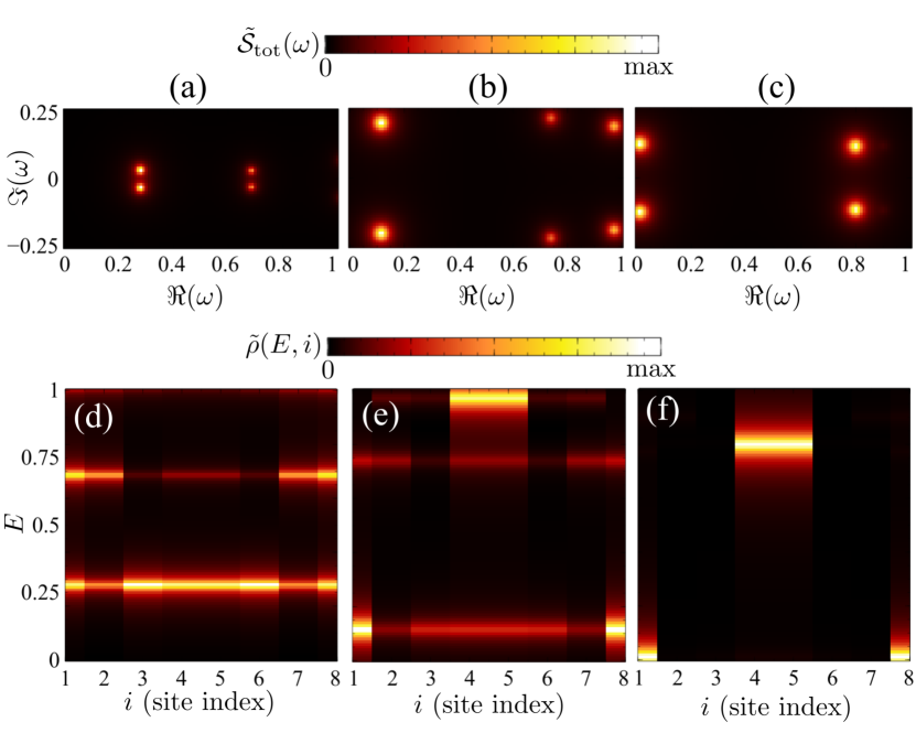
Figure S1: Spectral functions in Fig.1 in the main text, computed with exact diagonalization.

II Total density of states in Hatano-Nelson model with NHKPM

To show that the NHKPM faithfully computes spectral functions in the single particle case in the presence of non-Hermitian skin effect (NHSE), we consider the Hatano-Nelson model[4]:

$$H_{\text{HN}}=\sum_{l=1}^{L-1}(t+\gamma)c^{\dagger}_{l}c_{l+1}+(t-\gamma)c^{\dagger}_{l+1}c_{l},$$ (S35)

which exhibits NHSE when $\gamma\neq 0$. We compute the total density of states of the model:

$$\rho_{\text{tot}}(\omega)=\sum_{n}\delta(\Re(\omega-E_{n}))\delta(\Im(\omega-E_{n})).$$ (S36)

For simplicity we take $L=8$, and we note that analogous results can be obtained for larger $L$. The spectrum of $H_{\text{HN}}$ computed with ED with $t=1$ and $\gamma=0.4$ under periodic boundary condition (PBC) and open boundary condition (OBC) are shown in Figs.S2(a) and (d). We see that the PBC spectrum features a point gap, whereas the OBC spectrum is purely real. The spectrum computed with NHKPM in both cases are shown in Figs.S2(b) and (e), demonstrating the capability of NHKPM to provide faithful results in both cases. As discussed in the main text, the reason that NHKPM provides a faithful OBC spectrum in this case is due to the contribution of the zero modes of $\mathcal{H}$ to $G(E=0)$ when $\omega$ lies in the point gap of $H$. Due to finite-size effects, these zero modes have an exponentially small finite energy: $\mathcal{E}_{0}\propto\exp(-L/L_{0})$ where $L_{0}$ is a constant. According to Eq. (S34), to accurately capture the contribution of this zero mode to $G(E=0)$, we require:

$$\sigma=\frac{\pi}{N}\lesssim\frac{\mathcal{E}_{0}}{2\Delta},$$ (S37)

which for the exponentially small $\mathcal{E}_{0}$ requires an exponentially large $N$, hence the large $N$ in Figs.S2(e). When smaller $N$ is used, the computed spectrum becomes a pseudo-spectrum[5] under OBC (Fig.S2(f)) due to inaccurately accounting for the contribution of the zero mode to $G(E=0)$, while the spectrum under PBC only gets broadened (Fig.S2(c)). For comparison we also show the OBC spectrum computed with $\gamma=0$ (Fig.S2(g-i)), where only a broadening is observed for smaller $N$ due to the absence of NHSE.

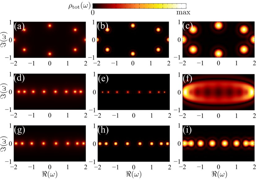
Figure S2: Total density of states $\rho_{\text{tot}}(\omega)$ defined in Eq. (S36) for $H_{\text{HN}}$ with $L=8$ and $t=1$, with (a) $\gamma=0.4$, under PBC, computed with ED, (b) $\gamma=0.4$, under PBC, computed with NHKPM with $N=100$, (c) $\gamma=0.4$, under PBC, computed with NHKPM with $N=50$, (d) $\gamma=0.4$, under OBC, computed with ED, (e) $\gamma=0.4$, under OBC, computed with NHKPM with $N=1000$, (f) $\gamma=0.4$, under OBC, computed with NHKPM with $N=50$, (g) $\gamma=0$, under OBC, computed with ED, (h) $\gamma=0$, under OBC, computed with NHKPM with $N=100$, and (i) $\gamma=0$, under OBC, computed with NHKPM with $N=50$.

III Entanglement entropy growth during the recursive calculations

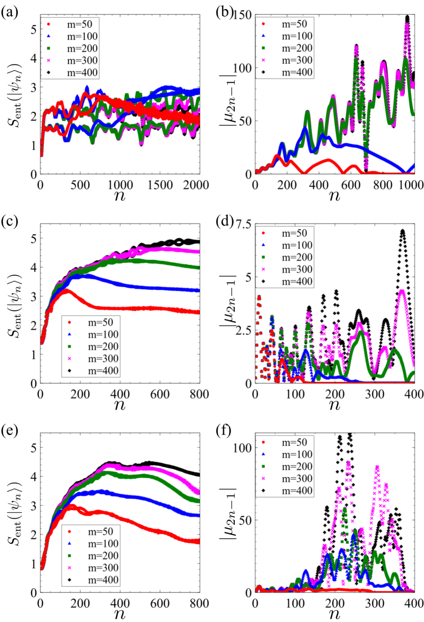
Figure S3: (a) Entanglement entropy of $|\psi_{n}\rangle$ and (b) the coefficients $|\mu_{2n-1}|$ in the iterative calculation Eq. (S24) for $H$ in Eq. (9) in main text with $h_{z}=\gamma=0$ and $\omega=0.1$. (c,d) Same as (a,b), but with $h_{z}=J$, $\gamma=0$ and $\omega=0.23i$. (e,f) Same as (a,b), but with $h_{z}=J$, $\gamma=0.1J$ and $\omega=0.23i$.

The updating of the states $|\psi_{n}\rangle$ in Eq. (S24) can result in states with large entanglement for large $n$ even if the initial state $|\psi_{\text{R}}\rangle$ is not much entangled. A largely entangled state would require larger bond dimensions in the matrix-product state (MPS) representation of the states, which increases computational cost. We analyze this entanglement increase in our calculation of the spectral function Eq.(4) for the Hamiltonian Eq.(9) in the main text, and we focus on the case $L=24$. For concreteness we choose $|\psi_{\text{L,R}}\rangle=S_{l}^{x}|\text{GS}_{\text{L,R}}\rangle$ with $l=12$, and the choice of $\omega$ is different in each specific case. We note that the results are qualitatively independent of the choice of site index $l$ and $\omega$.

The entanglement of a certain state $|\psi\rangle$ is characterized by the entanglement entropy at the middle of the chain $S_{\text{ent}}$, defined as

$$S_{\text{ent}}(|\psi\rangle)=\text{Tr}(\rho_{\text{A}}\log\rho_{\text{A}})$$ (S38)

$$\rho_{\text{A}}=\text{Tr}_{\text{B}}(|\psi\rangle\langle\psi|),$$ (S39)

where A and B are the left half and right half of the chain. The entanglement entropy defined in this way is meant to measure the numerical complexity to capture the wavefunction. In particular, for an MPS, it provides a lower bound for the bond dimension $m$[6]:

$$S_{\text{ent}}\leq S_{\text{max}}=-\sum_{i=1}^{m}\frac{1}{m}\log_{2}(\frac{1}{m})=\log_{2}m,$$ (S40)

where $S_{\text{max}}$ is the largest possible entanglement entropy of a bond of dimension $m$. Thus, a larger $S_{\text{ent}}$ indicates that a larger bond dimension is needed to accurately represent the state with MPS.

We first analyze $S_{\text{ent}}$ for $|\psi_{n}\rangle$ in the Hermitian case, and with different bond dimensions $m$ used in the MPS representation (Fig.S3(a)). It is first observed that for $m=50$ and $m=100$ the entanglement entropy starts to differ from results computed with a higher bond dimension at around $n=500$, indicating that $m$ is too small to accurately represent the state. Another observation is that the entanglement entropy saturates to a small value around 2 for large $n$, allowing the states to be represented accurately using a small $m$. As a consequence, the coefficients $\mu_{2n-1}$ computed with $m=200$ is accurate up to $n=600$, and with $m=300$ is accurate up to $n=1000$ (Fig.S3(b)). When a large non-Hermitian term $h_{z}=J$ is considered, the entanglement increase in the iterations becomes faster, and the entanglement entropy grows to a much larger value compared to the Hermitian case (Fig.S3(c)). As a consequence, the number of faithful coefficients drops for the same bond dimension $m$ used (Fig.S3(d)). In the Hermitian case, Figs.2(a,c) in the main text are computed with $N=500$ and $m=200$. In the case $h_{z}=J$, Figs.2(b,d) in the main text are computed with $N=300$ and $m=300$.

The presence of the non-Hermitian skin effect also results in a faster increase of entanglement entropy of $|\psi_{n}\rangle$ (Fig.S3(e)), and the faithful number of coefficients for fixed $m$ further drops (Fig.S3(f)). As a consequence, Fig.3(d) in the main text is computed with $N=200$ and $m=400$.

IV Numerical complexity of NHKPM

We analyze the numerical complexity of our algorithm in this section. In essence, an optimized version of our algorithm scales approximately as $L^{3}$, with $L$ the number of sites. This power law dependence makes our algorithm scalable to bigger systems. We elaborate on the details below.

We analyze the time consumption to compute the spectral function (Eq.(4) in the main text):

$$\begin{aligned} \mathcal{S}(\omega,l)=&\langle\text{GS}_{\text{L}}|S_{l}^{-}\delta^{2}(\omega+E_{\text{GS}}-H)S_{l}^{+}|\text{GS}_{\text{R}}\rangle\\ &+\langle\text{GS}_{\text{L}}|S_{l}^{+}\delta^{2}(\omega+E_{\text{GS}}-H)S_{l}^{-}|\text{GS}_{\text{R}}\rangle\end{aligned}$$ (S41)

with NHKPM for different system size $L$, where $H$ and $|\text{GS}_{\text{L},\text{R}}\rangle$ are given. In our particular case, the Hamiltonian $H$ is given by Eq.(9) in the main text, and $|\text{GS}_{\text{L},\text{R}}\rangle$ are computed with the Krylov-Schur algorithm. We focus on the topologically non-trivial regime: $h_{z}=J,\gamma=0$, and fix $\omega=0.23i$ and $l=1$ as the spectral function shows a peak at this point due to the topological edge excitations. We note that the energy mesh and a sweep over all sites required to compute the full spectral function can be easily parallelized. As a result, the scaling of the algorithm is determined by the size dependence for a fixed $\omega$ and $l$.

We fix the broadening of the peak for the scaling analysis. As the system size increases, a larger scaling factor $\Delta$ is required to scale the spectrum of $\mathcal{H}$ into $(-1,1)$. Thus, to ensure the same broadening, the number of polynomials $N$ should correspondingly increase. For our specific model, $\Delta$ is proportional to $L$, and thus we choose $N\propto L$ for the scaling analysis.

We first analyze the scaling of our algorithm for a generic case where the bond dimension of the MPS $m$ is fixed. In this case, the time consumption shows an approximately 3rd power dependence on the system size (Fig.5(a)). This scaling is the same as the kernel polynomial algorithm for Hermitian interacting systems[7].

We also analyze the scaling for our specific computation, where the entanglement entropy of states increases during the recursive calculations in the kernel polynomial method. In this case, to ensure the computational accuracy, a sufficiently large $m$ is required, which increases with $L$. In Fig.S5, we show the computed spectral functions as a function of $m$ for different sizes $L$. We show this for both $\omega=0.23i$ where the spectral function is dominated at the boundary, and for $\omega=0.8$ where the spectral function is dominated in the bulk. We observe that as $m$ increases, the computed spectral function approaches the accurate value as expected. We also observe that although the accuracy is low for small $m$, it is still clear that for $\omega=0.23i$ there exist edge excitations, and for $\omega=0.8$ the excitations are more distributed in the bulk. Thus, a relative error of $10\%$ is sufficient for the characterization of topological edge states. The smallest $m$ required for this accuracy is $m=40,50,60,80$ for $L=12,16,20,24$, respectively. For simplicity, we choose $m=10L/3$ to study the scaling, resulting in computational time $t\propto L^{5}$ (Fig.5(b)). Compared to the fixed $m$ case, the additional power of 2 originates from the fact that the complexity of applying a matrix product operator (MPO) on an MPS is proportional to $m^{2}$, and we have used $m\propto L$ in this case.

Figure S4: (a) Complexity of NHKPM algorithm with fixed bond dimension $m=80$ in MPS computations and $N=25L/2$, with $L_{0}=16$ and $t_{0}=442.9$s. The log-log data is fitted with a linear function, indicating that the complexity of the algorithm is power-law with $(t/t_{0})\propto(L/L_{0})^{2.8}$. (b) Complexity of NHKPM algorithm with bond dimension $m=10L/3$ in MPS computations and $N=25L/2$, with $L_{0}=12$ and $t_{0}=30.4$s. The log-log fit indicates a power-law complexity with $(t/t_{0})\propto(L/L_{0})^{5}$.

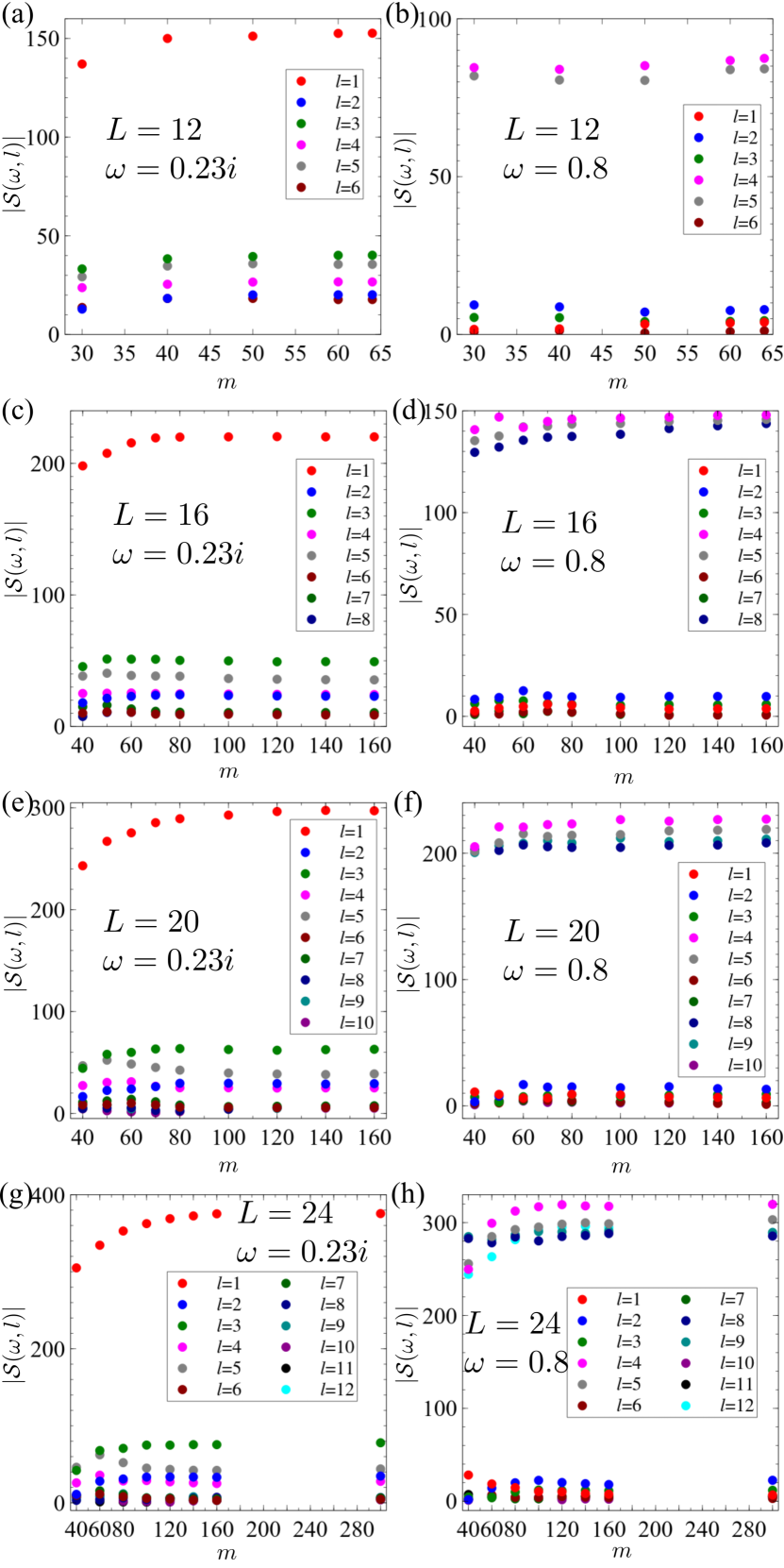
Figure S5: The spectral function $\mathcal{S}(\omega,l)$ computed for different $L$ and $\omega$ as a function of maximum bond dimension $m$. The parameters for $H$ (Eq. (9) in the main text) are $h_{z}=J$ and $\gamma=0$.

V Fidelity of ground states computed with the Krylov-Schur algorithm

The ground states are computed with the Krylov-Schur algorithm[8] in our case using matrix product state algebra. This method relies on an iterative algorithm to find the Krylov subspace expanded by a set of matrix-product states. Compared to generalized DMRG algorithms[9, 10, 11, 12], this method does not have the limitations given by the local updates of DMRG-like sweeps, and its accuracy is solely controlled by the bond dimension. In addition, it applies to arbitrary Hamiltonians without requiring specific symmetries, which is beneficial for studying Hamiltonians with generic ground states as in the case we studied.

We first compute the Krylov space expanded by 4 eigenvectors with the smallest real eigenvalue. We then identify the one with the smallest real eigenvalue out of the 4 as the ground state. In this way, we avoid the risk of mistaking an eigenvector with a similar eigenvalue to the ground state as the ground state. The calculated ground state is then verified by checking the deviations:

$$d_{\text{R}}(|\psi_{\text{R}}\rangle)=\frac{|\langle\psi_{\text{R}}|H^{\dagger}H|\psi_{\text{R}}\rangle|-|\langle\psi_{\text{R}}|H|\psi_{\text{R}}\rangle|^{2}}{|\langle\psi_{\text{R}}|H^{\dagger}H|\psi_{\text{R}}\rangle|}$$ (S42)

$$d_{\text{L}}(|\psi_{\text{L}}\rangle)=\frac{|\langle\psi_{\text{L}}|HH^{\dagger}|\psi_{\text{L}}\rangle|-|\langle\psi_{\text{L}}|H^{\dagger}|\psi_{\text{L}}\rangle|^{2}}{|\langle\psi_{\text{L}}|HH^{\dagger}|\psi_{\text{L}}\rangle|}.$$ (S43)

An exact right/left eigenvector $|\psi_{\text{R/L}}\rangle$ of $H$ should have $d_{\text{R}}(|\psi_{\text{R}}\rangle)=0$ and $d_{\text{L}}(|\psi_{\text{L}}\rangle)=0$. For $L=8$, $h_{z}=J$, $d_{\text{R}}(|\text{GS}_{\text{R}}\rangle)=1.4e{-5}$ and $d_{\text{L}}(|\text{GS}_{\text{L}}\rangle)=1.0e{-5}$; and when $h_{z}=2J$, $d_{\text{R}}(|\text{GS}_{\text{R}}\rangle)=9.7e-5$ and $d_{\text{L}}(|\text{GS}_{\text{L}}\rangle)=9.9e-5$. For $L=24$, $d_{\text{R}}(|\text{GS}_{\text{R}}\rangle)=3.0e-4$ and $d_{\text{L}}(|\text{GS}_{\text{L}}\rangle)=4.0e-4$ for $h_{z}=J,\gamma=0$, and $d_{\text{R}}(|\text{GS}_{\text{R}}\rangle)=7.2e-4$ and $d_{\text{L}}(|\text{GS}_{\text{L}}\rangle)=6.9e-4$ for $h_{z}=J,\gamma=0.1J$. Thus we have verified the ground states used in our calculation are faithful ground states.

References

- Note [1] Although is a complex-valued function, we can do Chebyshev expansion for its real and imaginary parts, respectively, then adding up the coefficients to get Eq. (S11\@@italiccorr).
- Weiße et al. [2006] A. Weiße, G. Wellein, A. Alvermann, and H. Fehske, The kernel polynomial method, Rev. Mod. Phys. 78, 275 (2006).
- Dawson [1897] H. G. Dawson, On the numerical value of , Proceedings of the London Mathematical Society s1-29, 519 (1897).
- Hatano and Nelson [1996] N. Hatano and D. R. Nelson, Localization transitions in non-hermitian quantum mechanics, Phys. Rev. Lett. 77, 570 (1996).
- Okuma and Sato [2020] N. Okuma and M. Sato, Hermitian zero modes protected by nonnormality: Application of pseudospectra, Phys. Rev. B 102, 014203 (2020).
- Schollwöck [2011] U. Schollwöck, The density-matrix renormalization group in the age of matrix product states, Annals of Physics 326, 96 (2011), january 2011 Special Issue.
- Lado and Zilberberg [2019] J. L. Lado and O. Zilberberg, Topological spin excitations in harper-heisenberg spin chains, Phys. Rev. Research 1, 033009 (2019).
- Stewart [2002] G. W. Stewart, A krylov–schur algorithm for large eigenproblems, SIAM Journal on Matrix Analysis and Applications 23, 601 (2002).
- Enss and Schollwöck [2001] T. Enss and U. Schollwöck, On the choice of the density matrix in the stochastic tmrg, Journal of Physics A: Mathematical and General 34, 7769 (2001).
- Chan and Van Voorhis [2005] G. K.-L. Chan and T. Van Voorhis, Density-matrix renormalization-group algorithms with nonorthogonal orbitals and non-hermitian operators, and applications to polyenes, The Journal of Chemical Physics 122, 204101 (2005).
- Zhang et al. [2020] D.-W. Zhang, Y.-L. Chen, G.-Q. Zhang, L.-J. Lang, Z. Li, and S.-L. Zhu, Skin superfluid, topological mott insulators, and asymmetric dynamics in an interacting non-hermitian aubry-andré-harper model, Phys. Rev. B 101, 235150 (2020).
- Yamamoto et al. [2022] K. Yamamoto, M. Nakagawa, M. Tezuka, M. Ueda, and N. Kawakami, Universal properties of dissipative tomonaga-luttinger liquids: Case study of a non-hermitian xxz spin chain, Phys. Rev. B 105, 205125 (2022).