Optimistic No-regret Algorithms for Discrete Caching

Abstract.

We take a systematic look at the problem of storing whole files in a cache with limited capacity in the context of optimistic learning, where the caching policy has access to a prediction oracle (provided by, e.g., a Neural Network). The successive file requests are assumed to be generated by an adversary, and no assumption is made on the accuracy of the oracle. In this setting, we provide a universal lower bound for prediction-assisted online caching and proceed to design a suite of policies with a range of performance-complexity trade-offs. All proposed policies offer sublinear regret bounds commensurate with the accuracy of the oracle. Our results substantially improve upon all recently-proposed online caching policies, which, being unable to exploit the oracle predictions, offer only $O(\sqrt{T})$ regret. In this pursuit, we design, to the best of our knowledge, the first comprehensive optimistic Follow-the-Perturbed leader policy, which generalizes beyond the caching problem. We also study the problem of caching files with different sizes and the bipartite network caching problem. Finally, we evaluate the efficacy of the proposed policies through extensive numerical experiments using real-world traces.

1. Introduction

This paper addresses the discrete caching (prefetching) problem: choose files to replicate in a local cache in order to maximize the probability that a new file request is served locally. Hitting the cache speeds up CPU, optimizes user experience in CDN’s (Bektas et al., 2007), and enhances the performance of wireless networks (Shanmugam et al., 2013). With the perpetual growth of Internet traffic fueled by new services such as AR/VR (D. Chatzopoulos, C. Bermejo, Z. Huang, and P. Hui, 2017), caching policies that learn fast to maximize cache hits can mitigate the increasing costs of information transportation (Paschos et al., 2018), and similar benefits can be expected for embedded and other computing systems (G. Gracioli, A. Alhammad, R. Mancuso, A. A. Frohlich, R. Pellizzoni, 2015). This work aspires to advance our theoretical understanding of this fundamental problem and proposes new provably-optimal and computationally-efficient caching algorithms using a new modeling and solution approach based on optimistic learning.

1.1. Motivation

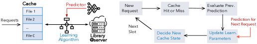
Figure 1. Optimistic online caching with predictions: system schematic (left) & algorithm template (right).

Common caching policies store the newly requested files and employ the Least-Recently-Used (LRU) (Jelenković and Kang, 2008), Least-Frequently-Used (LFU) (Lee et al., 1999) and other similar rules to evict files when the cache capacity is exhausted. Under certain statistical assumptions on the request trace, such policies maintain the cache at an optimal state, see (Paschos et al., 2020b, Sec. 3.1-3.2). However, with frequent addition of new content to libraries of online services and the high volatility of file popularity (Guillemin et al., 2013), these policies can perform arbitrarily bad. This has spurred intensive research efforts for policies that operate under more general conditions by learning on-the-fly the request distribution or adapting dynamically, e.g., with Reinforcement Learning, to observed requests; see Sec. 2. Nonetheless, these studies do not offer performance guarantees nor scale well for large libraries. The goal of this work is to design robust caching policies that are able to learn effective caching decisions with the aid of a prediction oracle of unknown quality (Fig. 1 left) even when the file requests are made in an adversarial fashion.

To that end, we formulate the caching problem as an online convex optimization (OCO) problem (Hazan, 2019). At each slot $t=1,2,\dots,T$, a learner (the caching policy) selects a caching vector $x_{t}\in\mathcal{X}$ from the set of admissible cache states $\mathcal{X}\subseteq\{0,1\}^{N}$ for a cache of size $C,$ where $N$ is the library size. Then, a $1$-hot vector $\theta_{t}\in\{0,1\}^{N}$ with value $1$ for the requested file is revealed, and the learner receives a reward of $f_{t}(x_{t})=\langle{\theta_{t}},{x_{t}}\rangle$ for cache hits. The reward is revealed only after committing $x_{t}$, which naturally matches the dynamic caching operation where the cached files are decided before the next request arrives. Here, the learner makes no statistical assumptions and $\theta_{t}$ can follow any distribution, even one that is handpicked by an adversary. In the optimistic framework, the learner does not only consider its hit or miss performance so far when deciding $x_{t}$, but also the predictor’s performance and output (Fig. 1 right). As customary in the online learning literature, we characterize the policy’s performance by using the static regret metric:

(1) $$R_{T}(\left\{x\right\}_{T})\triangleq\sup_{\{f_{t}\}_{t=1}^{T}}\left\{\sum_{t=1}^{T}f_{t}({x}^{\star})-\sum_{t=1}^{T}f_{t}({x}_{t})\right\},$$

where ${x}^{\star}\!=\!\operatorname*{argmax}_{x\in\mathcal{X}}\sum_{t=1}^{T}f_{t}({x})$ is the (typically unknown) best-in-hindsight cache decision that can be selected only with access to future requests. The regret measures the accumulated reward gap between the online decisions $\{x_{t}\}_{t}$ and benchmark $x^{\star}$. An algorithm is said to achieve sublinear regret when its average performance gap $R_{T}/T$ vanishes as $T\rightarrow\infty$. In this context, recent works have proposed caching policies that offer $O(\sqrt{T})$ regret bound (Bhattacharjee et al., 2020; Si Salem et al., 2021a, b; Paschos et al., 2020a; Mhaisen et al., 2022a; Paria and Sinha, 2021; Mhaisen et al., 2022b), which, in fact, is the optimal (as small as possible) achievable regret rate, see (Orabona, 2019, Thm. 5.1), (Bhattacharjee et al., 2020, Thm. 1).

Most of these regret-optimal algorithms have been designed for continuous caching, where it is assumed that each file is encoded and divided into a large number of small chunks such that storing them can be approximated by continuous variables (M. A. Maddah-Ali, and U. Niesen, 2014). In this case, the set of eligible caching states $\mathcal{X}$ is convex and hence one can readily apply standard OCO algorithms such as the Online Gradient Ascent (OGA). Albeit a handy assumption, there are settings where continuous caching cannot be used for practical reasons. Namely, keeping chunk meta-data consumes non-negligible storage; the coding operation is often computationally demanding; and the number of chunks might not be big enough to render continuous caching a good approximation. Therefore, we consider here the more realistic, and more challenging to solve, discrete caching problem. Indeed, in discrete caching the set $\mathcal{X}$ is naturally non-convex (containing binary file-caching decisions) and thus standard OCO policies cannot be employed. While first steps in the study of discrete caching, with equal-sized files, were recently made by (Si Salem et al., 2021a; Bhattacharjee et al., 2020; Paria and Sinha, 2021). In this paper, we extend their scope and design algorithms with substantially improved performance guarantees.

Namely, while regret minimization yields robust policies that learn under adversarial conditions, this framework receives the fair criticism that the policies have often suboptimal performance when the requests (cost functions, in general) are predictable, e.g., stationary. In such situations, we would like the policy to gauge the predictability of requests, and optimize aggressively the cache. For instance, requests in services like Facebook are often amenable to accurate forecasts; while in YouTube and Netflix the viewers receive recommendations which can effectively serve as predictions for their forthcoming requests (Gomez-Uribe and Hunt, 2016; Amatriain, 2012). Unfortunately, regret-based caching policies, such as (Paschos et al., 2020a; Si Salem et al., 2021b, a; Bhattacharjee et al., 2020; Paria and Sinha, 2021; Li et al., 2021), are pessimistically designed for the worst-case request sequence and cannot benefit from predictable requests. We tackle this shortcoming by designing a new suite of optimistic caching algorithms. An optimistic algorithm (Rakhlin and Sridharan, 2013; Mohri and Yang, 2016) has access to a prediction of an unknown quality for the next-slot utility function. The ultimate goal is to achieve constant (independent of $T$) regret when the predictions are accurate, while maintaining the worst-case regret bounds when predictions fail. This best-of-two-worlds approach, we show theoretically and demonstrate numerically, brings significant performance gains to dynamic caching.

1.2. Methodology and Contributions

We study key variants of the discrete caching problem, namely the single cache with equal or unequal-sized files and the bipartite caching, and propose a suite of optimistic learning algorithms with different pros and cons. Our first result demonstrates the best achievable regret in the setup we consider, which turns out to be $R_{T}=\Omega([\sum_{t}\|\theta_{t}-\tilde{\theta}_{t}\|]^{\nicefrac{{1}}{{2}}})$, indicating a significant potential of obtaining a regret that scales with the predictor’s error rather than the time horizon $T$ (Sec. 3). We then proceed to propose variants of the seminal Follow-The-Regularized-Leader (FTRL) and Follow-the-Perturbed-Leader (FTPL) algorithms, which can be both viewed as smoothing techniques for stabilizing learning decisions (Sec. 2.2), whose regret match this lower bound up to constants. In detail, we expand the optimistic FTRL algorithm (Mohri and Yang, 2016; Mhaisen et al., 2022b, a) that was designed for convex problems, to handle, through sampling, discrete (non-convex) decisions (Sec. 4). We prove this approach attains expected regret $O(\sqrt{T})$ for worst-case predictions and zero-regret for perfect predictions with an improved prefactor that does not depend on library size $N$. However, the OFTRL implementation can be hindered by an involved projection step that might be computationally expensive. Thus, we develop a new optimistic FTPL algorithm that applies prediction-adaptive perturbations to achieve a similar regret bound with linear ($O(N)$) computation overhead (Sec. 5). The flip side is that its regret bound contains $O(\textit{poly-log}(N))$ term.

We first derive results for equal-sized files, in line with all prior learning-based works for discrete caching (Bhattacharjee et al., 2020; Paria and Sinha, 2021; Lykouris and Vassilvtiskii, 2018; Rohatgi, 2020) or continuous caching (Paschos et al., 2020a; Mhaisen et al., 2022a; Si Salem et al., 2021a). Subsequently, we drop this assumption and study the single cache problem with different file sizes (Sec. 6). These first-of-their-kind regret-based algorithms require a point-wise approximation scheme for solving efficiently the NP-Hard Knapsack instance at each slot, while keeping the accumulated regret bound sublinear. To that end, we use the help of a rounding subroutine, DepRound (Byrka et al., 2017), to a known almost-discrete optimal solution Dantz (Dantzig, 1957). We show that the proposed policies achieve $(1/2)$-approximate regret of $O(\sqrt{T})$ and zero-regret for adversarial and perfect predictions, respectively. We also extend the OFTRL analysis to the widely used bipartite network caching model (Shanmugam et al., 2013; Paschos et al., 2018) (Sec. 7), where we optimize jointly the discrete caching and routing decisions to obtain prediction-modulated performance.

In (Sec. 8), we change tack and incorporate the optimism through the celebrated Experts model. The caching system in this case is a meta-learner which receives caching advice from an optimistic expert that suggests to cache solely w.r.t. predicted requests, and from a pessimistic expert that ignores predictions. We propose a tailored OGD-based scheme that allows the meta-learner to adapt to predictions’ accuracy ( performance of the optimistic expert) in a way that achieves negative regret when that expert is reliable, and, again, maintains an $O(\sqrt{T})$ regret for unreliable predictions.

In summary, we provide a comprehensive toolbox of algorithms having different computation overheads and performance, hence enabling practitioners to select the best approach to their problem. Moreover, we include technical results that are of independent interest, such as the non-convex OFTPL algorithm with improved regret bounds; the approximate non-convex OFTRL algorithm for the Knapsack problem; and an analysis of OFTRL/OFTPL with a probabilistic prediction model.

Notation. We denote sets with calligraphic capital letters, e.g., $\mathcal{N}=\{1,2,\ldots,N\}$; vectors with $x=(x_{i},i\in\mathcal{N})$ where $x_{i}$ is the $i$th component; and denote $x_{i}^{t}$ the $i$th component of the time-indexed vector $x_{t}$. The shorthand notation $x_{1:t}$ is used for $\sum_{i=1}^{t}x_{i}$. Also, $\{x_{t}\}_{t=1}^{k}$ denotes the sequence of vectors $\{x_{1},x_{2},\ldots,x_{k}\}$, and we use the succinct version $\{x_{t}\}_{T}$ for $\{x_{1},x_{2},\ldots,x_{T}\}$. When clear from context, we often drop the notation of actions and denote the regret $R_{T}(\left\{x\right\}_{T})$ simply with $R_{T}$.

2. Background and Related Work

2.1. Caching and Learning

Research on caching optimization spans several decades and we refer the reader to survey (Paschos et al., 2020b) for an introduction to the recent developments in this area. A large body of works focuses on offline policies which use the anticipated request pattern to proactively populate the caches with files that maximize the expected hits (Bektas et al., 2007). At the other extreme, dynamic caching solutions studied variants of the LFU/LRU policies (Jelenković and Kang, 2008; Lee et al., 1999; E. Leonardi, and G. Neglia, 2018; A. Giovanidis, and A. Avranas, 2016); tracked the request distribution (Traverso et al., 2013; Olmos et al., 2014) and optimized accordingly the caching (Leconte et al., 2016); employed reinforcement learning to adapt the caching decisions to requests (Sadeghi et al., 2018; Somuyiwa et al., 2018; Sadeghi et al., 2019); and, more recently, applied online convex optimization towards enabling the policies to handle unknown (adversarial) request patterns (Paschos et al., 2020a; Si Salem et al., 2021a; Mhaisen et al., 2022a; Bhattacharjee et al., 2020; Paria and Sinha, 2021; Si Salem et al., 2021b; Li et al., 2021). These latter works assume that the files can be fetched dynamically at each slot to optimize the cache configuration, as opposed to works such as (Lykouris and Vassilvtiskii, 2018; Rohatgi, 2020) which study pure eviction policies.

The interplay between predictions and caching has attracted attention from both machine learning and networking communities. The studies in (Chatzieleftheriou et al., 2019; Giannakas et al., 2021; Fu et al., 2022) formulated the joint caching and recommendation problem, considering static models, and assuming full knowledge of requests and the users’ propensity to follow recommendations (i.e., they place assumption on the prediction accuracy). On the other hand, (Lykouris and Vassilvtiskii, 2018; Rohatgi, 2020) presented a mechanism agnostic to requests that uses untrusted predictions to achieve competitive-ratio guarantees. Their approach was generalized to metrical task systems by (Antoniadis et al., 2020) and improved with nearly lower-bound matching for the competitive ratios in (Rutten et al., 2022). However, as proved in (Andrew et al., 2013), algorithms that ensure constant competitive-ratios do not necessarily guarantee sub-linear regret, which is the performance criterion we employ here following the recent regret-based caching research (Paschos et al., 2020a; Si Salem et al., 2021a; Mhaisen et al., 2022a; Bhattacharjee et al., 2020; Paria and Sinha, 2021; Si Salem et al., 2021b; Li et al., 2021). We note that all the above works consider files with equal size, while we extend the framework to the general scenario of unequally-sized files. In addition, none of the above works studies discrete caching with predictions. Finally, it is worth stressing that employing predictions for improving the performance of communication/computing systems is not a new idea: predictions have been incorporated in stochastic optimization (K. Chen, and L. Huang, 2018; X. Huang, S. Bian, X. Gao, W. Wu, Z. Shao, Y. Yang, J. C.S. Lui, 2021) which assume the requests and system perturbations are stationary; and in online learning (Z. Zhou, X. Chen, W. Wu, D. Wu, and J. Zhang, 2019; Comden et al., 2019) which do not adapt to predictions’ accuracy (considered known). Here, we make no assumptions on the predictions’ quality, which can be even adversarial.

2.2. Adaptive Smoothing

In contrast to the above studies, our optimistic learning approach is based on adaptive smoothing. Abernethy et. al. (Abernethy et al., 2014) introduced a unified view of FTRL and FTPL as techniques to add smoothing, through regularization or perturbation, to a non-smooth potential function. This perspective is useful to our work since we leverage both ideas. Namely, let us define: $\Phi(\theta)\triangleq{\max_{x\in\mathcal{X}}\langle{x},{\theta}\rangle}$, and consider the potential function $\Phi(\Theta_{t})$, where $\Theta_{t}=\theta_{1:t}$ is the vector of aggregated gradients (file requests). An intuitive strategy is to choose the action that maximizes the rewards seen so far:

(2) $$x_{t}=\operatorname*{argmax}_{x\in\mathcal{X}}\langle{\Theta_{t-1}},{x}\rangle=\nabla\Phi(\Theta_{t-1}),$$

which is known as Follow The Leader (FTL) and is optimal when the utility functions are samples from a stationary statistical distribution. In contrast, FTL has linear regret in the adversarial setting (Sachs et al., 2022; De Rooij et al., 2014), since successive gradients of non-smooth functions can be arbitrarily far from each other, thus leading to unstable actions. (Abernethy et al., 2014) proposed to stabilize the learner actions by smoothing the potential function, and selecting actions based on the smoothed potential $\nabla\tilde{\Phi}(\theta)$. In FTRL, the smoothing is achieved by adding a strongly convex function to the potential, i.e.,$x_{t}=\operatorname*{argmax}_{x\in\text{conv}(\mathcal{X})}\langle{x},{\Theta_{t}}\rangle-r_{1:t}(x)$

where $r_{t}(x)$ is a $\sigma_{t}$-strongly convex regularizer. This framework generalizes the Online Gradient Ascent (OGA) and the Exponentiated Weights (EG) algorithms, which were employed for the caching problem in (Paschos et al., 2020a) and (Si Salem et al., 2021a) respectively. As for FTPL, the smoothing is done by adding perturbation to the accumulated cost parameter of the potential. And the actions are decided by $x_{t}=\arg\max_{x\in\mathcal{X}}\langle{x},{\Theta_{t}+\eta_{t}\gamma}\rangle$,

where $\gamma\!\!\sim\!\!\mathcal{N}(0,\mathbf{1})$ and $\eta_{t}$ is a scaling factor that controls the smoothing. FTPL was shown to provide optimal regret guarantees for the discrete caching problem in (Bhattacharjee et al., 2020). Computationally efficiency is also a notable feature for FTPL updates as it requires an ordering operation instead of projection.

We propose to modulate the regularization $\sigma_{t}$ and perturbation $\gamma_{t}$ parameters with the predictions quality. Intuitively, accurate predictions should lead to less regularization/perturbation (less smoothing), enabling the learner to align its decisions more with the predictions. On the other hand, inaccurate predictions induce more smoothing, which alleviates their effects on the decisions. We show that careful tuning of these smoothing parameters leads to regret bounds that interpolate between $R_{T}\leq 0$, and $R_{T}\leq O(\sqrt{T})$. Nonetheless, these two algorithms have considerable differences in terms of computational complexity and constants in the bounds, which are discussed in detail.

2.3. Optimistic Learning

For regret minimization with predictions, (O. Dekel, 2017) used predictions $\theta_{t}$ for the gradient $\tilde{\theta}_{t}=\nabla f_{t}(x_{t})$ with guaranteed correlation $\langle{\tilde{\theta}_{t}},{\theta_{t}}\rangle\geq\alpha\|\theta_{t}\|^{2}$ to improve the regret . In (Bhaskara et al., 2020a), this assumption was relaxed to allow predictions to fail the correlation condition at some steps, obtaining bounds that interpolate between $O(\log(T))$ and $O(\sqrt{T})$; while this idea was extended to multiple predictors in (Bhaskara et al., 2020b). A different line of works (Rakhlin and Sridharan, 2013), (Mohri and Yang, 2016) use adaptive regularizers and define the $t$-slot prediction errors $\|\theta_{t}-\tilde{\theta}_{t}\|_{2}$ to obtain $O([\sum_{t}\|\theta_{t}-\tilde{\theta}_{t}\|^{2}]^{1/2})$ regret bounds. Specifically, OFTRL versions have been proposed in (Mohri and Yang, 2016) and recently used in (Anderson et al., 2022) for problems with budget constraints, while (Mhaisen et al., 2022a, b) tailored these ideas to continuous caching. The problem of discrete caching is fundamentally different. Through a careful analysis, we manage to reuse these results after relaxing the cache integrality constraints, and then employing a randomized rounding technique that recovers the same prediction-modulated regret in expectation. The regret bounds have the desirable property of being dimension-free. Nonetheless, we proceed to remark that OFTRL can have a computational bottleneck due to involving a projection step, which can be avoided in FTPL.

Optimistic versions of FTPL were recently investigated in (Suggala and Netrapalli, 2020b) and (Suggala and Netrapalli, 2020a). In (Suggala and Netrapalli, 2020b), the regret bound grows polynomially w.r.t. the decision set dimension. In the caching problem, this would imply a highly-problematic polynomial growth of the regret w.r.t. the typically huge library size $N$. The dependence of the regret on the dimension was improved in (Suggala and Netrapalli, 2020a), but it still remains linear. On the contrary, our proposed OFTPL exploits the structure of the decision set and utilizes adaptive perturbation to obtain a regret bound that depends on dimension only by $O(\log(N)^{1/4})$, is order-optimal (based on the achievable lower bound), returns zero-regret for perfect predictions, does not require knowing the time-horizon $T$, nor the prediction errors. None of these desirable features is available in these prior works. We kindly refer the reader to the table in Appendix. A.1 for an overview of the presented algorithms in the context of the most related literature.

3. Achievable regret for Caching with a Predictor

We first introduce a lower bound for the regret of any online caching policy $\pi$, working with a cache of capacity $C$, and has access to an untrusted and potentially adversarial prediction oracle. In general, the predictions refer to the next function $\tilde{f}_{t}(\cdot)$. However, since most OCO algorithms learn based on the observed gradients, it suffices to have predictions $\tilde{\theta}_{t}=\nabla\tilde{f}_{t}(x_{t})$. And for caching, this coincides with a prediction for the next request. Now, unlike all prior works in optimistic learning (Rakhlin and Sridharan, 2013; Mohri and Yang, 2016; Bhaskara et al., 2020a), we adopt here the more general probabilistic prediction model where $\tilde{\theta}_{t}$ is not necessarily a one-hot vector (as the actual $\theta_{t}$), but a probability distribution over the library. Thus, each $\tilde{\theta}_{t}$ is drawn from the N-dimensional probability simplex $\Delta_{N}$. This more general approach is rather intuitive as the forecasting models (e.g., a Neural Network) typically yield probabilistic inferences. It also enhances the performance of our optimistic algorithms and allows efficient training of the forecaster using a convex loss function (please see Appendix A.7.1 for examples and justification). It does require, however, a more elaborate technical analysis, especially for the case of OFTPL. In this setup, we have the following lower bound:

Theorem 1.

For any online caching policy $\pi$, there exist a sequence of requests $\{\theta_{t}\}_{T}$ and predictions $\{\tilde{\theta}_{t}\}_{T}$ for which the regret $R_{T}$ satisfies

(3) $$\mathop{\mathbb{E}}\left[{R_{T}}\right]\geq\sqrt{\frac{C}{2\pi}}\sqrt{\sum_{t=1}^{T}||\theta_{t}-\tilde{\theta}_{t}||_{2}^{2}}-\Theta\left(\frac{1}{\sqrt{T}}\right).$$

Proof.

To prove the lower bound, we show the existence of a request and prediction sequence under which the regret is guaranteed to be larger than the stated bound regardless of the online policy $\pi$. For that, we use the standard probabilistic method (Alon and Spencer, 2016) with an appropriately constructed random file request and prediction sequence as detailed below.

Denote by $\xi_{t}$ and $\tilde{\xi}_{t}$ the random variables representing the requested file ($\theta_{t}$) and its prediction ($\tilde{\theta}_{t}$) at time $t$, respectively. Denote by $\{X_{t}^{\pi}\}_{t\geq 1}$ the random variables representing the action of any policy $\pi$. We use a setup where $N\geq 2C$ and consider an ensemble of caching problems (i.e., request and prediction sequences) where at each slot $t$, the requested file $\xi_{t}$ is chosen independently and uniformly at random from the library $\mathcal{N}$. The predictions $\tilde{\xi}_{t}$ are also chosen independently and uniformly at random from the probability simplex $\Delta_{N}$. Specifically, we let

$$\{\tilde{\xi}_{t}\}_{t}\stackrel{{\scriptstyle\textrm{i.i.d.}}}{{\sim}}\textsc{Dirichlet}(\lambda_{1},\ldots,\lambda_{n},\ldots\lambda_{N})\quad\text{with}\quad\lambda_{n}=1,\forall n\in\mathcal{N}.$$

Hence, the expected reward obtained by any caching policy $\pi$ on any slot $t$, conditional on the information available to the policy can be bounded as

$$\mathbb{E}\left[\langle\xi_{t},X_{t}^{\pi}\rangle|\{\tilde{\xi}_{\tau}\}_{\tau=1}^{t},\{\xi_{\tau}\}_{\tau=1}^{t-1}\right] \stackrel{{\scriptstyle(a)}}{{=}}\mathbb{E}\mathbb{E}\left[\langle\xi_{t},X_{t}^{\pi}\rangle|\{\tilde{\xi}_{\tau}\}_{\tau=1}^{t},\{\xi_{\tau}\}_{\tau=1}^{t-1},X_{t}^{\pi}\right]$$

$$\stackrel{{\scriptstyle(b)}}{{=}}\frac{1}{2C}\mathbb{E}\bigg{[}\langle\bm{1},X_{t}^{\pi}\rangle|\{\tilde{\xi}_{\tau}\}_{\tau=1}^{t},\{\xi_{\tau}\}_{\tau=1}^{t-1},X_{t}^{\pi}\bigg{]}\stackrel{{\scriptstyle(c)}}{{\leq}}\frac{1}{2},$$

where $(a)$ follows from the tower property of expectations, $(b)$ from the fact $\xi_{t}\perp\big{(}\{\tilde{\xi}_{\tau}\}_{\tau=1}^{t},\{\xi_{\tau}\}_{\tau=1}^{t-1},X_{t}^{\pi}\big{)}$ and hence $\mathbb{E}(\xi_{t}|\{\tilde{\xi}_{\tau}\}_{\tau=1}^{t},\{\xi_{\tau}\}_{\tau=1}^{t-1},X_{t}^{\pi})=\mathbb{E}(\xi_{t})=\frac{1}{2C}\bm{1}_{N\times 1}$. Finally $(c)$ since $\langle\bm{1},X_{t}^{\pi}\rangle\leq C,$ which holds because of the cache capacity constraint. Taking expectation of the above bound, we have $\mathbb{E}[\langle\xi_{t},X_{t}^{\pi}\rangle]\leq\frac{1}{2}$. Hence, using the linearity of expectations, the expected value of the cumulative hits up to slot $T$ under any policy $\pi$ is upper bounded as $\mathbb{E}\big{[}\sum_{t=1}^{T}\langle\xi_{t},X_{t}^{\pi}\rangle\big{]}\leq\frac{T}{2}$.

Now we compute a lower bound to the expected number of cumulative hits achieved by the best-in-hindsight fixed cache configuration $X_{T}^{\star}$. Similar to (Bhattacharjee et al., 2020), we identify the problem with the classic setup of balls (requests) into bins (files). In this framework, it follows that the offline benchmark achieves cumulative hits which are equal to the total number of balls into the most-loaded $C$ bins when $T$ balls are thrown uniformly at random into $N=2C$ bins. Hence, from (Bhattacharjee et al., 2020, Lemma 1):

(4) $$\mathbb{E}\big{[}\sum_{t=1}^{T}\langle\xi_{t},X_{T}^{\star}\rangle\big{]}\geq\frac{T}{2}+\sqrt{\frac{CT}{2\pi}}-\Theta\left(\frac{1}{\sqrt{T}}\right).$$

Hence, the expected regret achieved by any policy in the optimistic set up is lower bounded as

(5) $$\mathbb{E}\left[R_{T}\right]=\mathbb{E}\bigg{(}\sum_{t=1}^{T}\langle\xi_{t},X_{T}^{\star}\rangle-\sum_{t=1}^{T}\langle\xi_{t},X_{t}^{\pi}\rangle\bigg{)}\geq\sqrt{\frac{CT}{2\pi}}-\Theta\left(\frac{1}{\sqrt{T}}\right).$$

Finally, we evaluate the expected value of the quantity $M_{T}\triangleq\sum_{t=1}^{T}\|\tilde{\xi}_{t}-\xi_{t}\|_{2}^{2}$ as follows.

(6) $$\mathbb{E}\left[M_{T}\right] =\mathbb{E}\left[\sum_{t=1}^{T}\|\tilde{\xi}_{t}-\xi_{t}\|_{2}^{2}\right]\stackrel{{\scriptstyle(a)}}{{=}}T\ \mathbb{E}\left[||\tilde{\xi}_{1}-\xi_{1}||_{2}^{2}\right]\stackrel{{\scriptstyle(b)}}{{=}}TN\ \mathbb{E}\left[(\tilde{\xi}^{1}_{1}-\xi^{1}_{1})^{2}\right]$$

(7) $$=TN\ \mathbb{E}\left[(\tilde{\xi}^{1}_{1})^{2}-2\tilde{\xi}^{1}_{1}\xi^{1}_{1}+(\xi^{1}_{1})^{2}\right]\stackrel{{\scriptstyle(c)}}{{=}}TN\bigg{[}\textrm{Var}(\tilde{\xi}_{1,1})+(\mathbb{E}(\tilde{\xi}_{1,1}))^{2}-2\mathbb{E}(\tilde{\xi}_{1,1})\mathbb{E}(\xi_{1,1})+\mathbb{E}(\xi^{2}_{1,1})\bigg{]}$$

(8) $$\stackrel{{\scriptstyle(d)}}{{=}}TN\bigg{[}\frac{(N-1)}{N^{2}(N+1)}+\frac{1}{N^{2}}-\frac{2}{N^{2}}+\frac{1}{N}\bigg{]}=T\big{(}1-\frac{2}{N(N+1)}\big{)}\leq T,$$

where $(a)$ follows from the i.i.d. assumption of the random vectors at each $t$, $(b)$ from the i.i.d assumption of each component of vectors $\tilde{\xi}_{1}$ and $\xi_{1}$, $(c)$ from $\xi_{t}\perp\tilde{\xi}_{t}$, and $(d)$ from standard results on Dirichlet distribution. Combining the above bound with (5), we have by Jensen’s inequality

$$\mathbb{E}\left[R_{T}\right]\geq\sqrt{\frac{C\mathbb{E}[M_{T}]}{2\pi}}-\Theta\left(\frac{1}{\sqrt{T}}\right)\geq\mathbb{E}\left[\sqrt{\frac{CM_{T}}{2\pi}}-\Theta\left(\frac{1}{\sqrt{T}}\right)\right]\quad\quad\quad\textit{i.e., }$$

$$\mathbb{E}\left[R_{T}-\sqrt{\frac{C\sum_{t=1}^{T}\|\tilde{\xi}_{t}-\xi_{t}\|_{2}^{2}}{2\pi}}\right]\geq-\Theta\left(\frac{1}{\sqrt{T}}\right)$$

From the above inequality, the result now follows from the standard probabilistic arguments. ∎

We will see that the proposed optimistic algorithms in Sections 4 and 5 attain this bound within an absolute and a poly-logarithmic factor, respectively.

4. Caching through Optimistic Regularization (OFTRL-Cache)

The first algorithm we propose is based on OFTRL. Prediction adaptive regularization was explored before in (Rakhlin and Sridharan, 2013) and later improved via proximal regularizers in (Mohri and Yang, 2016), all for convex sets. The gist of our approach is that we use OFTRL to obtain $\hat{x}_{t}\in\text{conv}(\mathcal{X}),\forall t$, and then apply Madow’s sampling scheme (Madow, 1949) to recover integral caching vectors $x_{t}\in\mathcal{X},\forall t,$ which satisfy the hard capacity non-convex constraint. In other words, we define:

(9) $$\mathcal{X}=\left\{{x}\in\left\{0,1\right\}^{N}\,\Bigg{|}\,\sum_{i=1}^{N}x_{i}\leq C\right\},$$

where $\mathcal{N}$ is the set of unit-sized files (library) and $C$ is the cache capacity (in file units); and $x_{i}\!=\!1$ decides to cache file $i\!\in\!\mathcal{N}$. Interestingly, despite having to operate on this non-convex set, this approach yields in expectation the same regret bounds as OFTRL for continuous caching (Mhaisen et al., 2022b).

1 Input: $\sigma=1/\sqrt{C}$, $\delta_{1}=\|\theta_{1}-\tilde{\theta}_{1}\|_{2}^{2}$, $\sigma_{1}=\sigma\sqrt{\delta_{1}}$, $x_{1}=\arg\min_{x\in\mathcal{X}}\langle{x},{\theta_{1}}\rangle$

2Output: $\{x_{t}\in\mathcal{X}\}_{T}$ $//$ Feasible discrete caching vector at each slot

3for  $t=2,3\ldots$  do

      4 $\tilde{\theta}_{t}\leftarrow\texttt{ prediction}$ $//$Obtain request prediction for slot $t$

      5 $\hat{x}_{t}=\operatorname*{argmax}_{x\in\text{conv}(\mathcal{X})}\left\{-r_{1:t-1}(x)+\langle{x},{\Theta_{t-1}+\tilde{\theta}_{t}}\rangle\right\}$ $//$ Update the continuous cache vector

      6 $x_{t}\leftarrow MadowSample(\hat{x}_{t})$ $//$ Obtain the discrete cache vector using Algorithm 7

      7 $\Theta_{t}=\Theta_{t-1}+\theta_{t}$ $//$ Receive $t$-slot request and update total gradient

      8 $\sigma_{t}=\sigma\left(\sqrt{\delta_{1:t}}-\sqrt{\delta_{1:t-1}}\right)$ $//$ Update the regularization parameter

      

end for

Algorithm 1 Optimistic Follow The Regularized Leader (OFTRL-Cache)

Let us define the prediction error at slot $t$ as $\delta_{t}\triangleq\|\theta_{t}-\tilde{\theta}_{t}\|_{2}^{2}$, and introduce the proximal $\sigma_{t}$-strongly convex regularizer w.r.t. the Euclidean $\ell_{2}$ norm:

(10) $$r_{t}(x)=\frac{\sigma_{t}}{2}\|x-x_{t}\|_{2}^{2}.$$

Following (Mhaisen et al., 2022a), we define parameters $\{\sigma_{t}\}_{t}$ using the accumulated prediction errors, namely:

(11) $$\sigma_{1}=\sigma\sqrt{\delta_{1}},\quad\quad\quad\sigma_{t}=\sigma\left(\sqrt{\delta_{1:t}}-\sqrt{\delta_{1:t-1}}\right)\quad\forall t\geq 2,\quad\text{with}\quad\sigma=1/\sqrt{C}.$$

The basic OFTRL update stems from using these regularizers in the FTRL update formula. Namely, at each slot $t$ we update the cache to maximize the aggregated utility. This maximization is regularized through a term (the above-defined regularizers) that depends on the predictor’s accuracy.

The detailed steps are summarized in Algorithm 1. In the first iteration we draw randomly a feasible caching vector $x_{1}$ and observe the prediction error $\delta_{1}=\|\theta_{1}-\tilde{\theta}_{1}\|_{2}^{2}$. In each iteration we need to solve a strongly convex program (line 5) which returns the continuous caching vector $\hat{x}_{t}$, that is transformed to a feasible discrete $x_{t}$ (line 6) using Madow’s Sampling (see Appendix A.2). The algorithm notes the new gradient vector, by simply observing the next request, and updates the accumulated gradient $\Theta_{t}$ (line 7). The regret guarantee of Algorithm 1 is described next.

Theorem 1.

Algorithm 1 ensures, for any time horizon $T$ and $N\geq 2C$, the expected regret bound:

$$\mathbb{E}[R_{T}]\leq 2\sqrt{C}\sqrt{\sum_{t=1}^{T}\|\theta_{t}-\tilde{\theta}_{t}\|_{2}^{2}}$$

Proof.

We define first the regret w.r.t. the continuous actions $\{\hat{x}_{t}\}_{T}$ as $\hat{R}_{T}\triangleq\langle{\Theta_{T}},{x^{\star}}\rangle-\sum_{t=1}^{T}\langle{\theta_{t}},{\hat{x}_{t}}\rangle$, where $x^{\star}$ is the optimal-in-hindsight caching vector. We also define the scaled Euclidean $\ell_{2}$ norm $\|\cdot\|_{(t)}=\sqrt{\sigma_{1:t}}\ \|\cdot\|_{2}$ so that $r_{1:t}$ is 1-strongly convex w.r.t $\|\cdot\|_{(t)}$, and note that its dual norm is $\|\cdot\|_{(t),\star}=\frac{1}{\sqrt{\sigma_{1:t}}}\ \|\cdot\|_{2}$. Our starting point is (Mhaisen et al., 2022a, Lem. 1), which we restate below:

Lemma 0.

Let $r_{1:t}$ be a 1-strongly convex w.r.t. a norm $\|\cdot\|_{(t)}$. Then, the OFTRL iterates produced by line $5$ in Algorithm 1 guarantee the bound $\hat{R}_{T}\leq r_{1:T}(x^{\star})+\frac{1}{2}\sum_{t=1}^{T}\|\theta_{t}-\tilde{\theta}_{t}\|^{2}_{(t),\star}$.

Now, we first get a deterministic regret bound on $\hat{x}_{t}$. Assuming that $C\in(0,N/2]$, we can bound the $\ell_{2}$ diameter of the caching set as $\|x^{\star}-x_{t}\|_{2}\leq\sqrt{2C},\forall x^{\star},x_{t}\in\text{conv}(\mathcal{X})$. Thus, we can upper-bound the regularizers in (10), replace in the above Lemma and telescope to get:

(12) $$\hat{R}_{T}\leq\sigma_{1:T}\ C+\frac{1}{2}\sum_{t=1}^{T}\frac{\delta_{t}}{\sigma_{1:t}}.$$

Observing that the sum $\sigma_{1:t}$ telescopes to $\sigma\sqrt{\delta_{1:t}}$, we can substitute it in (12) and use the standard identity (Orabona, 2019, Lem. 4.13) to bound the second term via $\sum_{t=1}^{T}\delta_{t}/\sqrt{\delta_{1:t}}\leq 2\sqrt{\delta_{1:T}}$. Therefore, we obtain: $\hat{R}_{T}\leq\sigma\sqrt{\delta_{1:T}}\ C+\frac{1}{\sigma}\sqrt{\delta_{1:T}}$, and by setting the parameter $\sigma$ to its optimal value $\sigma=1/\sqrt{C}$, we can eventually write:

(13) $$\hat{R}_{T}\leq 2\sqrt{C}\sqrt{\sum_{t=1}^{T}\|\theta_{t}-\tilde{\theta}_{t}\|_{2}^{2}}.$$

The last step requires Madow’s sampling (line 6). By construction, the routine selects $C$ files and hence returns a feasible integral caching vector $x_{t}$ (or, sampled vector). In addition, each item is included in the sampled vector with a probability based on the continuous $\hat{x}_{t}$. Namely, it holds $\Pr(x_{i}^{t}=1)=\pi_{i}-\pi_{i-1}=\hat{x}_{i}^{t}$, where the auxiliary parameter $\pi_{i}$ aggregates the (interpreted as) probabilities for caching the first $i$ files, i.e., $\pi_{i}=\sum_{k=0}^{i}\hat{x}_{k}$. Since each $x_{i}^{t}$ is binary, it holds $\mathbb{E}[x_{t}]\!=\!\Pr(x_{i}^{t}\!=1)\!=\!\hat{x}_{t}$. The result follows by using (13) and observing:

(14) $$\vspace{-1mm}\mathop{\mathbb{E}}\left[{R_{T}\left(\{x\}_{T}\right)}\right]=\langle{\Theta_{T}},{x^{\star}}\rangle-\mathop{\mathbb{E}}\left[{\sum_{t=1}^{T}\langle{\theta_{t}},{x_{t}}\rangle}\right]=\hat{R}_{T}.$$

∎

Discussion. The bound in Theorem 1 ensures the desirable prediction-based modulation of the algorithm’s performance, as the achieved regret shrinks with the prediction quality. If all predictions are accurate, we get $R_{T}\leq 0$; when all predictions fail, we get $R_{T}\leq 2\sqrt{2CT}$. That is, in the worst scenario (e.g., when the predictions are created by an adversary) the regret bound is worse by a constant factor of $\sqrt{2}$ compared to the FTRL algorithm that does not use predictions (McMahan, 2017, Sec. 3.4)), and $\sim 5$ compared to the lower bound derived in Sec. 3. Moreover, due to selecting an $\ell_{2}$ regularizer, the bounds are dimension-free and do not depend on the library size $N$. This is particularly important since in caching problems oftentimes the library size is an even bigger concern than the time horizon. Finally, note that the algorithm does not need to know the horizon $T$ beforehand. The drawback of this optimistic caching approach is the computational complexity of the iteration (line 5) which involves a projection operation. While $\ell_{2}$ projections have received attention (Hazan, 2019, Sec. 7), they can hamper the scalability of the algorithm under certain conditions. In the following section we show how perturbation-based smoothing can avoid the projection step.

5. Caching through Optimistic Perturbations (OFTPL-Cache)

We propose next a new OFTPL algorithm that significantly improves previous OFTPL proposals (Suggala and Netrapalli, 2020b, a), both in terms of their bounds and implementation, and as such is of independent interest with potential applications that extend beyond caching to other $k-$set structured problems such as those discussed in (Cohen and Hazan, 2015). The improvement is possible by setting the perturbation parameters $\eta_{t}$ in a manner that is adaptive to prediction error witnessed until $t-1$.

1 Input: $\eta_{1}=0$, $y_{1}=\arg\min_{y\in\mathcal{X}}\langle{y},{\theta_{1}}\rangle$

2Output: $\{y_{t}\in\mathcal{X}\}_{T}$ $//$ Feasible discrete caching vector at each slot

3$\gamma\stackrel{{\scriptstyle iid}}{{\sim}}\mathcal{N}(0,\bm{1}_{N\times 1})$ $//$ Sample a perturbation vector

4 for  $t=2,3,\ldots$  do

      5 $\tilde{\theta}_{t}\leftarrow\texttt{ prediction}$ $//$Obtain request prediction for slot $t$

      6 $\eta_{t}=\frac{1.3}{\sqrt{C}}\left(\frac{1}{\ln(Ne/C)}\right)^{\frac{1}{4}}\sqrt{\sum_{\tau=1}^{t-1}\|\theta_{\tau}-\tilde{\theta}_{\tau}\|^{2}_{1}}$ $//$ Update the perturbation parameter

      7 $y_{t}=\operatorname*{argmax}_{y\in\mathcal{X}}\langle{y},{\Theta_{t-1}+\tilde{\theta}_{t}+\eta_{t}\gamma}\rangle$ $//$ Update the discrete cache vector

      8 $\Theta_{t}=\Theta_{t-1}+\theta_{t}$ $//$ Receive the request for slot $t$ and update total gradient

end for

Algorithm 2 Optimistic Follow The Perturbed Leader (OFTPL-Cache)

Following the discussion in Sec. 2, we remind the reader that the FTPL actions are derived by solving in each slot $t$ a linear program (LP) with a parameterized perturbed cumulative utility vector, $\Theta_{t-1}+\eta_{t}\gamma$, where $\eta_{t}\in\mathbb{R}_{+}$ is the perturbation parameter. In order to obtain the optimistic FTPL variant we introduce two twists: (i) the prediction for the next-slot utility $\tilde{\theta}_{t}$ is added to the cumulative utility; and (ii) the perturbation parameter $\eta_{t}$ is scaled according to the accumulated prediction error. Interestingly, due to the structure of the decision set $\mathcal{X}$, the LP solution reduces to identifying the $C$ files with the highest coefficients. This step can be efficiently implemented in deterministic linear $(O(N))$ time using, e.g., the Median-of-Medians algorithm (Cormen et al., 2022). The steps of the proposed scheme are presented in Algorithm 2, where we denote the $t$-slot OFTPL decisions with $y_{t}\in\mathcal{X}$. The following theorem characterizes the performance of this new OFTPL algorithm.

Theorem 1.

Algorithm 2 ensures, for any time horizon $T$ and $N\geq 2C$ with $C\geq 11$, the expected regret bound:

(15) $$\mathbb{E}_{\gamma}[R_{T}]\leq 3.68\sqrt{C}\ \bigg{(}\ln\frac{Ne}{C}\bigg{)}^{1/4}\sqrt{\sum_{t=1}^{T}||\theta_{t}-\tilde{\theta}_{t}||_{1}^{2}}.$$

Proof.

We consider the following baseline potential function $\Phi(\theta)\triangleq{\max_{y\in\mathcal{X}}\langle{y},{\theta}\rangle}$, which is a sub-linear function. The associated Gaussian smoothed potential function for each $t$, is defined as:

(16) $$\Phi_{t}(\theta)\triangleq\mathop{\mathbb{E}}_{\gamma\sim\mathcal{N}(0,I)}\left[{\max_{y\in\mathcal{X}}\langle{y},{\theta+\eta_{t}\gamma}\rangle}\right]=\mathop{\mathbb{E}}_{\gamma}\left[{\Phi(\theta+\eta_{t}\gamma)}\right]$$

Clearly, $\Phi_{t}(\theta)$ is convex in $\theta$. Recall that the cumulative file request vector is defined as $\Theta_{t}=\Theta_{t-1}+\theta_{t}.$ A Taylor expansion of $\Phi_{t}(\cdot)$ around the point $\Theta_{t-1}+\tilde{\theta}_{t}$, evaluated at $\Theta_{t}$, with a second order remainder is:

(17) $$\Phi_{t}(\Theta_{t})=\Phi_{t}(\Theta_{t-1}+\tilde{\theta}_{t})+\langle{\nabla\Phi_{t}(\Theta_{t-1}+\tilde{\theta}_{t})},{\theta_{t}-\tilde{\theta}_{t}}\rangle+\frac{1}{2}\langle{\theta_{t}-\tilde{\theta}_{t}},{\nabla^{2}\Phi_{t}(\hat{\theta}_{t})\ (\theta_{t}-\tilde{\theta}_{t})}\rangle,$$

where $\hat{\theta}_{t}$ is a point on the line segment connecting $\Theta_{t}$ and $\Theta_{t-1}+\tilde{\theta}_{t}$. From the convexity of $\Phi_{t}(\cdot)$:

(18) $$\Phi_{t}(\Theta_{t-1}+\tilde{\theta}_{t})\leq\Phi_{t}(\Theta_{t-1})+\langle{\nabla\Phi_{t}(\Theta_{t-1}+\tilde{\theta}_{t})},{\tilde{\theta}_{t}}\rangle.$$

From (17) and (18), we can eventually write:

(19) $$\Phi_{t}(\Theta_{t})\leq\Phi_{t}(\Theta_{t-1})+\langle{\nabla\Phi_{t}(\Theta_{t-1}+\tilde{\theta}_{t})},{\theta_{t}}\rangle+\frac{1}{2}\langle{\theta_{t}-\tilde{\theta}_{t}},{\nabla^{2}\Phi_{t}(\hat{\theta}_{t})(\theta_{t}-\tilde{\theta}_{t})}\rangle.$$

Now, note that it holds $\nabla\Phi_{t}(\Theta_{t-1}+\tilde{\theta}_{t})=$

(20) $$\nabla\mathop{\mathbb{E}}_{\gamma}\left[{\Phi_{t}(\Theta_{t-1}+\tilde{\theta}_{t})}\right]\stackrel{{\scriptstyle(a)}}{{=}}\mathop{\mathbb{E}}_{\gamma}\left[{\nabla\Phi_{t}(\Theta_{t-1}+\tilde{\theta}_{t})}\right]=\mathop{\mathbb{E}}_{\gamma}\left[{\arg\max_{y\in\mathcal{X}}\langle{y},{\Theta_{t-1}+\tilde{\theta}_{t}+\eta_{t}\gamma}\rangle}\right]=\mathop{\mathbb{E}}_{\gamma}\left[{y_{t}}\right],$$

where $(a)$ stems from (Bertsekas, 1973, Prop. 2.2). Thus, $\eqref{eq:te2}$ can be written as:

(21) $$\Phi_{t}(\Theta_{t})\leq\Phi_{t}(\Theta_{t-1})+\mathop{\mathbb{E}}_{\gamma}\left[{\langle{\theta_{t}},{y_{t}}\rangle}\right]+\frac{1}{2}\langle{\theta_{t}-\tilde{\theta}_{t}},{\nabla^{2}\Phi_{t}(\hat{\theta}_{t})(\theta_{t}-\tilde{\theta}_{t})}\rangle.$$

Subtracting $\Phi_{t-1}(\Theta_{t-1})$ from both sides and telescoping over $T$ and setting $\eta_{0}=0$, we get:

(22) $$\Phi_{T}(\Theta_{T})\leq\sum_{t=1}^{T}\left(\Phi_{t}(\Theta_{t-1})-\Phi_{t-1}(\Theta_{t-1})+\mathop{\mathbb{E}}_{\gamma}\left[{\langle{\theta_{t}},{y_{t}}\rangle}\right]+\frac{1}{2}\langle{\theta_{t}-\tilde{\theta}_{t}},{\nabla^{2}\Phi_{t}(\hat{\theta}_{t})(\theta_{t}-\tilde{\theta}_{t})}\rangle\right).$$

Then, by Jensen’s inequality: $\max_{y\in\mathcal{X}}\mathop{\mathbb{E}}_{\gamma}\left[{\langle{y},{\Theta_{T}+\eta_{T}\gamma}\rangle}\right]=\max_{y\in\mathcal{X}}{\langle{y},{\Theta_{T}}\rangle}=\Phi(\Theta_{T})\leq\Phi_{T}(\Theta_{T})$, and writing the last term as the norm of the vector $(\theta_{t}-\tilde{\theta}_{t})$ induced by the symmetric positive semidefinite matrix $\nabla^{2}\Phi_{t}(\hat{\theta}_{t})\triangleq H_{t}$, we get the following upper bound of the regret:

(23) $$R_{T}\leq\Phi(\Theta_{T})-\sum_{t=1}^{T}\mathop{\mathbb{E}}_{\gamma}\left[{\langle{\theta_{t}},{y_{t}}\rangle}\right]\leq\sum_{t=1}^{T}\left(\Phi_{t}(\Theta_{t-1})-\Phi_{t-1}(\Theta_{t-1})+\frac{1}{2}\|\theta_{t}-\tilde{\theta}_{t}\|_{H_{t}}\right).$$

We now bound the first term in the RHS of inequality (23):

$$\sum_{t=1}^{T}\!\Phi_{t}(\Theta_{t-1})\!-\!\Phi_{t-1}(\Theta_{t-1})=\sum_{t=1}^{T}\!\mathop{\mathbb{E}}_{\gamma}\left[{\Phi(\Theta_{t-1}\!+\eta_{t}\gamma)-\Phi\left(\Theta_{t-1}\!+\eta_{t-1}\gamma\right)}\right]\stackrel{{\scriptstyle(a)}}{{\leq}}\!\sum_{t=1}^{T}\mathop{\mathbb{E}}_{\gamma}\left[{\Phi\left((\eta_{t}\!-\eta_{t-1})\gamma\right)}\right]$$

(24) $$\stackrel{{\scriptstyle(b)}}{{\leq}}\sum_{t=1}^{T}(\eta_{t}-\eta_{t-1})\mathop{\mathbb{E}}_{\gamma}\left[{\Phi(\gamma)}\right]{\leq}\eta_{T}\mathop{\mathbb{E}}_{\gamma}\left[{\max_{y}\langle{y},{\gamma}\rangle}\right]\stackrel{{\scriptstyle(c)}}{{\leq}}\eta_{T}\sqrt{2C\ln\binom{N}{C}}\stackrel{{\scriptstyle(d)}}{{\leq}}\eta_{T}C\sqrt{2\ln(Ne/C)},$$

where inequalities $(a)$ and $(b)$ follow from the sub-linearity of the potential function; $(c)$ from Massart’s lemma which gives an upper bound the expected sum of the top $C$ elements in a Gaussian random vector (e.g., (Cohen and Hazan, 2015, Lem. 9)); and finally $(d)$ is due to $\binom{N}{C}\leq(\frac{Ne}{C})^{C}$.

We now upper bound the second term in the RHS of (23). From (Cohen and Hazan, 2015, Eqn. (4)), the $(i,j)$^th entry of the Hessian matrix is given by $H^{t}_{i,j}=\frac{1}{\eta_{t}}\mathbb{E}\big{[}\tilde{y}(\hat{\theta}_{t}+\eta_{t}\gamma)_{i}\gamma_{j}\big{]},$ where $\tilde{y}(\cdot)=\arg\max_{y\in\mathcal{X}}\langle{y},{\cdot}\rangle$. Hence, we have the following bound on the absolute value of each entry:

(25) $$|H^{t}_{i,j}|=\frac{1}{\eta_{t}}\left|\mathop{\mathbb{E}}_{\gamma}\left[{\tilde{y}(\hat{\theta}+\eta_{t}\gamma)_{i}\gamma_{j}}\right]\right|\leq\frac{1}{\eta_{t}}\mathop{\mathbb{E}}_{\gamma}\left[{|\tilde{y}(\hat{\theta}+\eta_{t}\gamma)_{i}|\ |\gamma_{j}|}\right]\leq\frac{1}{\eta_{t}}\mathop{\mathbb{E}}_{\gamma}\left[{|\gamma_{i}|}\right]\leq\frac{1}{\eta_{t}}\sqrt{\frac{2}{\pi}},$$

where the first inequality follows from Jensen’s inequality, the second holds since $\tilde{y}_{i}=\{0,1\}$; and the last one is a property of Gaussian r.v.s. Thus each of the quadratic forms on the RHS of Eqn. (23) can be bounded as follows:

(26) $$\|\theta_{t}-\tilde{\theta}_{t}\|_{H_{t}}=\langle{\theta_{t}-\tilde{\theta}_{t}},{H_{t}(\theta_{t}-\tilde{\theta}_{t})}\rangle=\sum_{i,j}(\theta_{t,i}-\tilde{\theta}_{t,i})H^{t}_{ij}(\theta_{t,j}-\tilde{\theta}_{t,j})$$

(27) $$\stackrel{{\scriptstyle(a)}}{{\leq}}\sum_{i,j}|(\theta_{t,i}-\tilde{\theta}_{t,i})||H^{t}_{ij}||(\theta_{t,j}-\tilde{\theta}_{t,j})|\stackrel{{\scriptstyle(b)}}{{\leq}}\frac{1}{\eta_{t}}\sqrt{\frac{2}{\pi}}(\sum_{i}|(\theta_{t,i}-\tilde{\theta}_{t,i})|)^{2}=\frac{1}{\eta_{t}}\sqrt{\frac{2}{\pi}}||\theta_{t}-\tilde{\theta}_{t}||_{1}^{2}.$$

where $(a)$ follows from the triangle inequality and $(b)$ from the bound (25).

Another way to bound $\|\theta_{t}-\tilde{\theta}_{t}\|_{H_{t}}$, which will be useful later, starts from (17) to get:

$$\frac{1}{2}\|\theta_{t}-\tilde{\theta}_{t}\|_{H_{t}}=\Phi_{t}(\Theta_{t})-\Phi_{t}(\Theta_{t-1}+\tilde{\theta}_{t})-\langle{\nabla\Phi_{t}(\Theta_{t-1}+\tilde{\theta}_{t})},{\theta_{t}-\tilde{\theta}_{t}}\rangle$$

$$=\mathop{\mathbb{E}}_{\gamma}\left[{\Phi(\Theta_{t}+\eta_{t}\gamma)-\Phi(\Theta_{t-1}+\tilde{\theta}_{t}+\eta_{t}\gamma)}\right]+\langle{\nabla\Phi_{t}(\Theta_{t-1}+\tilde{\theta}_{t})},{\tilde{\theta}_{t}-\theta_{t}}\rangle\stackrel{{\scriptstyle(a)}}{{\leq}}\Phi(\theta_{t}-\tilde{\theta}_{t})+$$

(28) $$+\langle{\nabla\Phi_{t}(\Theta_{t-1}+\tilde{\theta}_{t})},{\tilde{\theta}_{t}-\theta_{t}}\rangle=\max_{y\in\mathcal{X}}\langle{y},{\theta_{t}-\tilde{\theta}_{t}}\rangle+\langle{\nabla\Phi_{t}(\Theta_{t-1}+\tilde{\theta}_{t})},{\tilde{\theta}_{t}-\theta_{t}}\rangle\stackrel{{\scriptstyle(b)}}{{\leq}}2\|\theta_{t}-\tilde{\theta}_{t}\|_{1},$$

where $(a)$ follows from the sub-additivity of $\Phi(\cdot)$, and in $(b)$ we use that $y_{i}\in\{0,1\},\forall i$ and bounded both terms using triangle inequality. Hence, combining the bounds (27) and (28), we get:

(29) $$\frac{1}{2}\|\theta_{t}-\tilde{\theta}_{t}\|_{H_{t}}\leq\min\Big{(}\frac{1}{\sqrt{2\pi}}\frac{||\theta_{t}-\tilde{\theta_{t}}||_{1}^{2}}{\eta_{t}},2||\theta_{t}-\tilde{\theta_{t}}||_{1}\Big{)}.$$

Now we choose the learning rate $\eta_{t}=\beta\sqrt{\sum_{\tau=1}^{t-1}||\theta_{\tau}-\tilde{\theta}_{\tau}||_{1}^{2}},t\geq 1$ for some constant $0<\beta\leq\frac{1}{\sqrt{2\pi}}$ that will be specified later. Hence, we have:

(30) $$\!\!\!\!\!\frac{1}{2}\|\theta_{t}\!-\tilde{\theta}_{t}\|_{H_{t}}\!\leq\!\min\left(\frac{||\theta_{t}\!-\tilde{\theta_{t}}||_{1}^{2}}{\sqrt{2\pi}\beta\sqrt{\sum_{\tau=1}^{t-1}||\theta_{\tau}\!-\tilde{\theta}_{\tau}||_{1}^{2}}},2\frac{||\theta_{t}-\tilde{\theta_{t}}||^{2}_{1}}{\sqrt{2\pi}\beta\sqrt{||\theta_{t}\!-\tilde{\theta_{t}}||^{2}_{1}}}\right)\!\stackrel{{\scriptstyle(a)}}{{\!\leq\!}}\frac{3}{\sqrt{2\pi}\beta}\frac{||\theta_{t}\!-\tilde{\theta_{t}}||^{2}_{1}}{\sqrt{\sum_{\tau=1}^{t}||\theta_{\tau}\!-\tilde{\theta}_{\tau}||_{1}^{2}}}\!\!$$

where in $(a)$, we used the fact that $\min(a_{1}/a_{2},b_{1}/b_{2})\leq\frac{a_{1}+a_{2}}{b_{1}+b_{2}}$ for any two positive fractions and $\sqrt{x+y}\leq\sqrt{x}+\sqrt{y},$ for any non-negative $x$ and $y$’s.

Now that we have a bound for the smoothing-overhead in (24), and the per-step regret bounds (30), we can substitute them in (23) to get:

(31) $$\mathop{\mathbb{E}}_{\gamma}\left[{R_{T}}\right]\leq{\eta_{T}C\sqrt{2\log(Ne/C)}}+\frac{3}{\sqrt{2\pi}\beta}{\sum_{t=1}^{T}\frac{||\theta_{t}-\tilde{\theta_{t}}||^{2}_{1}}{\sqrt{\sum_{\tau=1}^{t}||\theta_{\tau}-\tilde{\theta}_{\tau}||_{1}^{2}}}}.$$

The second term above can be upper-bounded as:

(32) $$\sum_{t=1}^{T}\frac{||\theta_{t}-\tilde{\theta_{t}}||^{2}_{1}}{\sqrt{\sum_{\tau=1}^{t}||\theta_{\tau}-\tilde{\theta}_{\tau}||_{1}^{2}}} \leq\sum_{t=1}^{T}\int_{\sum_{\tau=1}^{t-1}||\theta_{\tau}-\tilde{\theta}_{\tau}||_{1}^{2}}^{\sum_{\tau=1}^{t}||\theta_{\tau}-\tilde{\theta}_{\tau}||_{1}^{2}}\frac{dx}{\sqrt{x}}=\int_{0}^{\sum_{\tau=1}^{T}||\theta_{\tau}-\tilde{\theta}_{\tau}||_{1}^{2}}\frac{dx}{\sqrt{x}}=2\sqrt{\sum_{\tau=1}^{T}||\theta_{\tau}-\tilde{\theta}_{\tau}||_{1}^{2}}.$$

Substituting the above bound into (31) and using the definition of $\eta_{T}$ we get the regret upper bound:

(33) $$\mathbb{E}_{\gamma}[R_{T}]\leq\sqrt{\sum_{\tau=1}^{T}||\theta_{\tau}-\tilde{\theta}_{\tau}||_{1}^{2}}\bigg{(}C\sqrt{2\ln(Ne/C)})\beta+\frac{6}{\beta\sqrt{2\pi}}\bigg{)}$$

Optimizing over the constant $\beta$, we get that $\beta=\sqrt{\frac{3}{C}}(\frac{1}{\pi\ln(Ne/C)})^{\nicefrac{{1}}{{4}}}$, $C\geq 11$ (Recall we that $0<\beta\leq 1/\sqrt{2\pi}$). Substituting this valud for $\beta$ back in (33) we arrive at the result.∎

Discussion. Similarly to Theorem 1, the regret bound here is modulated with the quality of predictions: it collapses to zero when predictions are perfect, and maintains $R_{T}\!\leq\!3.68\ \ln\left(\frac{Ne}{C}\right)^{1/4}\sqrt{2CT}$ for arbitrary bad predictions. Interestingly, this worst-case scenario is only inferior by a factor of $\sim 2.5$ compared to the recent FTPL algorithm in (Bhattacharjee et al., 2020) that does not use (and cannot benefit from) predictions. Hence, incorporating predictions (even, of unknown quality) comes without cost in the proposed OFTPL algorithm. Furthermore, for the more common case of predictions within a certain range of error, the regret bounds diminish in proportion to their quality.

Comparing with Theorem 1, OFTPL achieves regret bounds worse by a factor of $\sim 1.9\ln\left(\frac{Ne}{C}\right)^{1/4}$, which depends on $N$, albeit in a small order. The regret bounds are also different in nature, for OFTRL it is $\ell_{2}$ squared whereas for OFTPL, it is the much larger $\ell_{1}$ squared of the prediction error. On the other hand, Algorithm 2 does not involve the expensive projection operation that appears in Algorithm 1, but rather a simple quantile-finding operation (top $C$ files) with a worst-case complexity of $O(N)$. This facilitates greatly the implementation of OFTPL in systems with low computing capacity or in applications that require decisions in near real-time. A notable point about Theorem 1 is that in the special case where the predictor $\tilde{\theta_{t}}$ suggests a single file (i.e., deterministic), the regret scales with the square root of the number of mistakes as opposed to the conventional number of time slots (i.e., horizon $T$) in previous no regret discrete caching works(Bhattacharjee et al., 2020; Si Salem et al., 2021a; Paria and Sinha, 2021). It is also interesting to note that the bounds of Theorem 1, and 1, provide insights on the appropriate loss function to be optimized by the prediction oracle (squared norms). This is helpful while training and tuning machine learning models on request traces detests. Lastly, we note that we can sample a fresh perturbation vector at each time step in order to handle adaptive adversaries (i.e., adversaries that do not fix the cost sequence in advance but react to the choices of the algorithm). The same analysis applies since perturbations are equal in distribution. We refer the reader to e.g., (Hutter and Poland, 2005, Sec. 8) for techniques for reducing guarantees from oblivious to adaptive adversaries via fresh-sampling.

6. Caching files with Arbitrary Sizes

While the caching problem with equal-sized files has been studied using regret analysis and competitive analysis, to the best of the authors’ knowledge, there are no results for the more challenging case of files with different sizes. This section fills this gap by extending the above tools accordingly. In particular, we consider the setting where each file $i\in\mathcal{N}$ has a size of $s_{i}$ units, $s_{i}\leq C$. Hence, the set of feasible caching vectors needs to be redefined as:

(34) $$\mathcal{X}_{s}=\left\{{x}\in\left\{0,1\right\}^{N}\bigg{|}\sum_{i=1}^{N}s_{i}x_{i}\leq C\right\},$$

where the caching decisions are calibrated with the respective file sizes in the capacity constraint. And similarly, the benchmark (designed-in-hindsight) policy is redefined as $x^{\star}=y^{\star}\triangleq\operatorname*{argmax}_{x\in\mathcal{X}_{s}}\langle x,\Theta_{T}\rangle$. We present two solution approaches for this problem, using both OFTRL and OFTPL. These results are of independent interest with applications beyond caching.

6.1. Approximate OFTPL

Similarly to Algorithm 2, the OFTPL algorithm in this case determines the next cache configuration $y_{t}$ by solving the following integer programming problem at each round $t$:

(35) $$\mathbb{P}_{1}:\qquad\max_{y\in\mathcal{X}_{s}}\,\,\langle\Theta_{t-1}+\tilde{\theta_{t}}+\eta_{t}\gamma,y\rangle,$$

which is a Knapsack instance with profit vector $p=\Theta_{t-1}+\tilde{\theta}_{t}+\eta_{t}\gamma$; size vector $s=\left(s_{i},\forall i\in\mathcal{N}\right)$; and capacity $C$. Since the Knapsack problem is NP-Hard (Martello and Toth, 1990), we cannot solve $\mathbb{P}_{1}$ efficiently (fast and accurately) at each slot, and hence it is not practical (or, even possible) to use the approach of Sec. 5. Instead, we resort here to an approximation scheme for solving $\mathbb{P}_{1}$ and, importantly, do so in a way that these approximately-solved instances do not accumulate an unbounded regret w.r.t. $y^{\star}$. This requires a tailored approximation analysis and to define a new regret metric.

In detail, we leverage Dantzig’s approach for tackling packing problems (Dantzig, 1957), to obtain an almost-integral solution from the respective integrality-relaxed problem; and then recover, via a point-wise randomized rounding, a fully-integral solution which, as we prove, keeps the long-term $\nicefrac{{1}}{{2}}$-approximate regret bounded. First, recall that the $\alpha$-approximate regret is defined as (Kalai and Vempala, 2005):

(36) $$R_{T}^{(\alpha)}\triangleq\alpha\langle{\Theta_{T}},{x^{\star}}\rangle-\sum_{t=1}^{T}\langle{\theta_{t}},{x_{t}}\rangle,$$

for a positive constant $\alpha$. This generalized regret metric allows to use a parameterized benchmark, in line with prior works, e.g., see (Paria and Sinha, 2021) and references therein. Now, it is important to see that while the Knapsack problem admits an FPTAS (Vazirani, 2001), due to the online nature of our caching problem, not all $\alpha$-approximation schemes for the offline OFTPL problem provide an $\alpha$-approximate regret guarantee. In light of this, we employ the stronger notion of point-wise $\alpha$-approximation scheme, which yields an $\alpha$-regret guarantee for the online learning problem (Kalai and Vempala, 2005). We restate the definition:

Definition 0 ($\alpha$-point-wise approximation).

A randomized $\alpha$-point-wise approximation algorithm $\mathcal{A}$ for a fractional solution $\hat{y}=(\hat{y}_{i},i\in\mathcal{N})$ of a maximizing LP with non-negative coefficients, is one that returns an integral solution $y=(y_{i},i\in\mathcal{N})$ such that $\mathop{\mathbb{E}}\left[{y_{i}}\right]\geq\alpha\hat{y_{i}},\forall i\in\mathcal{N}$ and some $\alpha>0$; where the expectation is taken over possible random choices made by algorithm $\mathcal{A}$.

In our case, we set $\alpha=1/2$ and propose an $(\nicefrac{{1}}{{2}})$-point-wise approximation algorithm for $\mathbb{P}_{1}$.

Our starting point is Dantzig’s approach which operates on the integrality-relaxed version of $\mathbb{P}_{1}$. In particular, the integrality-relaxed LP for the Knapsack problem with profit vector $p$, weight vector $s$, and capacity $C$, through the following steps:

Dantz$(C,p,s)$:

1. Index files in decreasing profit-to-size ratios, i.e., $({p_{1}}/{s_{1}})\geq({p_{2}}/{s_{2}})\geq\ldots\geq({p_{N}}/{s_{N}})$.

2. Set $k=\min\big{\{}j\,\big{|}\,\sum_{i=1}^{j}s_{i}>C\big{\}}$ and $\widetilde{C}=C-\sum_{i=1}^{k-1}s_{i}$.

3. Assign the continuous variables $\hat{y}_{i}\in[0,1],i\in\mathcal{N}$ as follows:

   $$\hat{y}_{i}=\begin{cases}1,~{}~{}\,\,\,\textrm{if}\,\,\,~{}i\in[k-1]\\ \frac{\widetilde{C}}{s_{k}},~{}~{}\textrm{if}\,\,\,~{}i=k\\ 0,~{}~{}\,\,\,\textrm{otherwise}.\end{cases}$$

To streamline presentation, we denote with Dantz$(C,p,s)$ the operation of steps (1)-(3) above on the Knapsack instance $(C,p,s)$, which return the solution $\hat{y}$ and the value of parameter $k$. An interesting property of returned solution $\hat{y}$, which we exploit in our randomized approximation scheme, is that at most one component of the vector $\hat{y}$ is non-integral.

1 Input: $\eta_{1}=0$, $y_{1}=\arg\min_{y\in\mathcal{X}_{s}}\langle{y},{\theta_{1}}\rangle$, $s=(s_{i},i\in\mathcal{N})$

2 Output: $\{y_{t}\in\mathcal{X}_{s}\}_{T}$   $//$ Feasible discrete caching vector at each slot

3$\gamma\stackrel{{\scriptstyle iid}}{{\sim}}\mathcal{N}(0,\bm{1}_{N\times 1})$ $//$ Sample a perturbation vector

4 for  $t=2,3,\ldots$  do

      5 $\tilde{\theta}_{t}\leftarrow\texttt{ prediction}$ $//$Obtain request prediction for slot $t$

      6 $\eta_{t}=\frac{1.3}{\sqrt{C}}\left(\frac{1}{\ln(Ne/C)}\right)^{1/4}\sqrt{\sum_{\tau=1}^{t-1}\|\theta_{\tau}-\tilde{\theta}_{\tau}\|^{2}_{1}}$ $//$ Update the perturbation parameter

      7 $p\leftarrow\Theta_{t-1}+\tilde{\theta}_{t}+\eta_{t}\gamma$ $//$ Update the profit vector

      8 $(\hat{y}_{t},k)\leftarrow$ Dantz$(C,p,s)$ $//$ Compute the ”almost integral” cache vector

      9 $y_{t}\leftarrow$ Rand$(\hat{y}_{t},k)$ $//$ Perform Randomized Rounding

      10 $\Theta_{t}=\Theta_{t-1}+\theta_{t}$ $//$ Receive $t$-slot request and update total grad

end for

Algorithm 3 OFTPL-UneqCache

The detailed steps of the proposed OFTPL scheme are presented in Algorithm 3. At each slot we obtain a new (probabilistic) prediction for the next requested file $\tilde{\theta}_{t}$ (line 5) and update the perturbation parameter $\eta_{t}$ (line 6). Then we calculate the new profits $p_{i}=\Theta_{t-1}+\tilde{\theta}_{t}+\eta_{t}\gamma$, $i\in\mathcal{N}$, and solve the relaxed Knaspack by invoking Dantz$(C,p,s)$ to obtain the almost-integral $\hat{y}_{t}$ and parameter $k$ (line 7). This vector has $k-1$ components equal to 1, one additional non-negative component, and $N-k$ components equal to 0. This solution is then rounded through the randomization scheme:

Rand$(\hat{y}_{t},k)$:

1. Set $S={1,2,\ldots,k-1}\triangleq[k-1]$ with probability $\nicefrac{{1}}{{2}}$; Set $S=\{k\}$ with probability $\nicefrac{{1}}{{2}}$.

2. Set $y^{t}_{i}=0,\forall i\in\mathcal{N}$; and update to $y^{t}_{i}=1$ for each $i\in S$.

The Rand operation is invoked and creates integral caching vector $y_{t}$ which satisfies the capacity constraint (line 9). Finally, we observe the new gradient, update the aggregate gradient vector and repeat the process (line 10). The following theorem, proved in Appendix. A.4, characterizes the guarantees of Algorithm 3.

Theorem 2.

Algorithm 3 ensures, for any time horizon $T$, the expected regret bound:

$$\mathop{\mathbb{E}}\left[{R^{(\nicefrac{{1}}{{2}})}_{T}}\right]\leq 1.84\sqrt{C}\left(\ln{\frac{Ne}{C}}\right)^{1/4}\sqrt{\sum_{t=1}^{T}\|\theta_{t}-\tilde{\theta}_{t}\|_{1}^{2}}$$

Discussion. The bounds of Theorem 3 possess the desirable property of being modulated with the prediction errors, and in fact are improved by a factor of half compared to the equal-sizes bound. However, we remind the reader that the regret metric in this section is defined w.r.t. a weaker benchmark, i.e., a benchmark that achieves $\nicefrac{{1}}{{2}}$ the utility of the best-in-hindsight utility $\langle\Theta_{T},y^{\star}\rangle$. Relying upon such approximations is an inevitable concession for NP-hard problems – especially when having to solve them repeatedly. Interestingly, the computational complexity of Algorithm 3 is comparable to that of Algorithm 2, which is quite surprising since we are able to handle integral caching decisions with arbitrary-sized files. To the best of the authors’ knowledge, this work is the first to propose an OCO-based solution for this variant of the online caching problem. We proceed next to remove the effect of the library size on the regret bound.

6.2. Approximate OFTRL

We introduce next an OFTRL algorithm that can handle arbitrary file sizes. To that end, we use the OFTRL update on the integrality-relaxed version of the problem, then modify the obtained vector so as to be almost integral, and finally employ the same randomized rounding technique as above to correct for feasibility. The new intermediate step (that yields the almost-integral vector) is necessary since, unlike in Sec. 6.1, we cannot apply the $(\nicefrac{{1}}{{2}})$-sampling technique directly on $\{\hat{x}_{t}\}_{t}$ because these vectors do not have this required almost-integral form. Thus, we leverage the DepRound subroutine from (Byrka et al., 2017), which is known to achieve the useful property re-stated below.

Lemma 0.

For $a\in[0,1]^{N}$, the DepRound scheme in Algorithm 8 returns a vector $b$ such that

• All elements of $b$ are integral except one: $b_{i}\in\{0,1\}$ $\forall i\in\mathcal{N}/j$, $b_{j}\in[0,1]$.

• $b_{i}$ is an unbiased estimator of $a_{i}$: $\mathop{\mathbb{E}}\left[{b_{i}}\right]=a_{i},\forall i\in\mathcal{N}$.

• $b$ respects the linear constraints satisfied by $a$: $\Pr[\sum_{i\in\mathcal{N}}s_{i}\ a_{i}=\sum_{i\in\mathcal{N}}s_{i}\ b_{i}]=1$.

With this almost-integral solution at hand, we re-use the sampling technique Rand, to achieve an $(\nicefrac{{1}}{{2}})$-Regret guarantee w.r.t. the same benchmark as in Sec. 6.1. The steps are presented in Algorithm 4. The diligent reader will observe that essentially we merge steps from Algorithm 1 and Algorithms 3. The detailed steps of the DepRound subroutine are presented in the Appendix. The next theorem, proved in the Appendix A.5, characterizes the algorithm’s performance.

1 Input: $\sigma=1/\sqrt{C}$, $\delta_{1}=\|\theta_{1}-\tilde{\theta}_{1}\|_{2}^{2}$, $\sigma_{1}=\sigma\sqrt{\delta_{1}}$, $x_{1}=\arg\min_{x\in\mathcal{X}_{s}}\langle{x},{\theta_{1}}\rangle$

2 Output: $\{y_{t}\in\mathcal{X}_{s}\}_{T}$   $//$ Feasible discrete caching vector at each slot

3for  $t=2,3,\ldots$  do

      4 $\tilde{\theta}_{t}\leftarrow\texttt{ prediction}$ $//$Obtain gradient prediction for slot $t$

      5 $\hat{x}_{t}=\arg\max_{x\in\text{conv}(\mathcal{X}_{s})}\left\{-r_{1:t-1}(x)+\langle{x},{\Theta_{t-1}+\tilde{\theta}_{t}}\rangle\right\}$

      6 $\bar{x}_{t}\longleftarrow$ DepRound$(\hat{x}_{t})$ $//$ Compute the ”almost integral” cache vector

      7 $x_{t}\longleftarrow$ Rand$(\bar{x}_{t},k)$ $//$ Perform Randomized Rounding

      8 $\Theta_{t}=\Theta_{t-1}+\theta_{t}$ $//$ Receive $t$-slot request and update total grad

      9 $\sigma_{t}=\sigma\left(\sqrt{\delta_{1:t}}-\sqrt{\delta_{1:t-1}}\right)$ $//$ Update the regularization parameter

      

end for

Algorithm 4 OFTRL-UneqCache

Theorem 4.

Algorithm 4 ensures, for any time horizon $T$, the expected regret bound:

$$\mathop{\mathbb{E}}\left[{R_{T}^{(\nicefrac{{1}}{{2}})}}\right]\leq\sqrt{C}\sqrt{\sum_{t=1}^{T}\|\theta_{t}-\tilde{\theta}_{t}\|_{2}^{2}}$$

Discussion. Compared to the approach we used to extend OFTPL to unequal-sized files, an additional rounding technique (DepRound) was necessary to extend OFTRL. The complexity of this sub-routine is linear in the library size. Thus, despite preserving the order-level complexity of Algorithm 4, handling such files increases the overhead to get the almost-integral caching vectors $\{\bar{x}_{t}\}_{t}$. The important point is that we recover the dimension-free bounds for the regret, which are better by a constant factor of $1.84\left(\ln\frac{Ne}{C}\right)^{1/4}$ compared to OFTPL-UneqCache, at the expense of performing a (potentially challenging) projection step. Hence, one can select the most suitable method depending on the requirements of the application (size of library, slot length, etc.) and the computing resources when executing the algorithm. Lastly, in Algorithm 4, and all introduced algorithms for the single cache case, the request vector $\theta$ can be extended to include (time-varying and unknown) weights that depend on users or network properties.

7. Bipartite Caching Through Optimism (OFTRL-BipCache)

Finally, we extend our study to caching networks where a set of edge caches ${\mathcal{J}}=\{1,2,\dots,J\}$ serves a set of users ${\mathcal{I}}=\{1,2,\dots,I\}$ requesting files from the library $\mathcal{N}$. The connectivity between $\mathcal{I}$ and $\mathcal{J}$ is modeled with parameters $d=\big{(}d_{ij}\in\{0,1\}:i\!\in\!\mathcal{I},j\in\mathcal{J}\big{)}$, where $d_{ij}=1$ if cache $j$ can be reached from user location $i$. Each user can be (potentially) served by any connected cache. This is a widely-studied non-capacitated bipartite model (Paschos et al., 2020b; Shanmugam et al., 2013).

We introduce the new caching variables $k$ and routing variables $u$. Namely, $k_{nj}^{t}\!\in\!\{0,1\}$ decides whether file $n\!\in\!\mathcal{N}$ is stored at cache $j\!\in\!\mathcal{J}$ at the beginning of slot $t$, and the $t$-slot caching vector $k_{t}\!=\!(k_{nj}^{t}:n\!\in\!\mathcal{N},j\!\in\!\mathcal{J})$ belongs to $\mathcal{K}=\left\{k\in\{0,1\}^{N\cdot J}~{}\big{|}~{}\sum_{n\in\mathcal{N}}k_{nj}\leq C_{j},~{}j\in\mathcal{J}\right\},$ where $C_{j}$ is the capacity of cache $j\in\mathcal{J}$. We use the routing variable $u_{nij}^{t}\in\{0,1\}$ to decide the delivery of file $n$ to user $i$ from cache $j$, and define the $t$-slot routing vector $u_{t}=(u_{nij}^{t}\!\in\![0,1]:n\!\in\!\mathcal{N},i\!\in\!\mathcal{I},j\!\in\!\mathcal{J})$ that is selected from the set: $\mathcal{U}=\left\{u\in\{0,1\}^{N\cdot J\cdot I}~{}\big{|}~{}\sum_{j\in\mathcal{J}}u_{nij}\leq 1,~{}n\in\mathcal{N},i\in\mathcal{I}\right\}.$ Note also that unserved requests, i.e., when the summation is strictly smaller than $1$, are satisfied by the root cache. This option, however, yields zero benefit for the users (no cache-hit gains); see also (Shanmugam et al., 2013). The request vector $\theta_{t}$ is redefined to reflect a request’s source and destination: $\theta_{t}\!=\!(\theta_{ni}^{t}\!\in\!\{0,1\}:n\!\in\!\mathcal{N},i\!\in\!\mathcal{I})$, and is drawn from the set: $\mathcal{Q}=\left\{\theta\in\{0,1\}^{N\cdot I}~{}\big{|}~{}\sum_{n\in\mathcal{N}}\sum_{i\in\mathcal{I}}\theta_{ni}=1\right\}.$

1 Input: $\sigma=1/\sqrt{1+JC}$, $\delta_{1}=\|\theta_{1}-\tilde{\theta}_{1}\|_{2}^{2}$, $\sigma_{1}=\sigma\sqrt{\delta_{1}}$, $x_{1}=\arg\min_{x\in\mathcal{X}_{b}}\langle{x},{\theta_{1}}\rangle$

2Output: $\{x_{t}=(k_{t},u_{t})\in\mathcal{X}_{b}\}_{T}$  $//$ Feasible discrete caching/routing vector at each slot

3for  $t=2,3,\ldots$  do

      4 $\tilde{\theta}_{t}\leftarrow\texttt{ prediction}$ $//$Obtain request prediction for slot $t$

      5 $\hat{x}_{t}=\arg\max_{x\in\text{conv}(\mathcal{X}_{b})}\left\{-r_{1:t-1}(x)+\langle{x},{\Theta_{t-1}+\tilde{\theta}_{t}}\rangle\right\}$ $//$ Update the continuous policy vector

      6 $(k_{j}^{t})\longleftarrow MadowSample(\hat{k}_{t})$, $\forall j\in\mathcal{J}$ $//$ Obtain the discrete cache vector for each cache independently

      7 $\Theta_{t}=\Theta_{t-1}+\theta_{t}$ $//$ Receive $t$-slot request and update total grad

      8 Set $u^{t}_{nij^{\prime}}\leftarrow 1$ for a randomly selected $j^{\prime}\in\mathcal{J}^{ni}$ $//$Update the discrete routing vector

      9 $\sigma_{t}=\sigma\left(\sqrt{\delta_{1:t}}-\sqrt{\delta_{1:t-1}}\right)$ $//$ Update the regularization parameter

      

end for

Algorithm 5 OFTRL-BipCache

We can now introduce the $t$-slot utility function:

(37) $$f_{t}(x_{t})=\sum_{n\in\mathcal{N}}\sum_{i\in\mathcal{I}}\sum_{j\in\mathcal{J}}\theta^{t}_{ni}k_{nij}^{t}\ .$$

where we abuse notation and redefine $x_{t}\triangleq(k_{t},u_{t})$. Therefore, the utility-maximizing caching-routing policy at each slot $t$ is found by solving the following problem:

(38) $$\mathbb{P}_{2}:\,\,\max_{x}\,\,\, \sum_{t=1}^{T}f_{t}(x)\,\,\,\,\,\,\,\text{s.t.}\,\,\,\,\,\,u\in\mathcal{U},\,\,\,\,k\in\mathcal{K};\,\,\,\,u_{nij}\leq k_{nj}d_{ij},\,i\in\mathcal{I},j\in\mathcal{J},n\in\mathcal{N},$$

and we define the feasible caching/routing set as $\mathcal{X}_{b}\triangleq\left\{\{\mathcal{K}\times\mathcal{U}\}\cap\{u_{nij}\leq k_{nj}d_{ij}\}\right\}$. $\mathbb{P}_{2}$ is known to be NP-Hard via a reduction to the set cover problem (Shanmugam et al., 2013, Sec. 3), (Paria and Sinha, 2021, Sec. 4.1). Hence, we will be using below also its integrality-relaxed version $\mathbb{P}_{2}^{\prime}$ with continuous variables $\hat{x}_{t}\triangleq(\hat{k}_{t},\hat{u}_{t})$.

Our strategy for tackling $\mathbb{P}_{2}$ is to use OFTRL on the convex hull of $\mathcal{X}_{b}$ (essentially learning w.r.t. $\mathbb{P}_{2}^{\prime}$) to optimize $\hat{x}_{t}$, and then obtain discrete caching vectors with Madow’s sampling applied to each cache separately. As last step we select a proper routing solution for the received request $\theta_{t}$. Namely, upon receiving a request for file $n$ from user $i$, the corresponding routing variable is set to $1$ if any cache connected to $i$ stores file $n$. Thus, we define the auxiliary set $\mathcal{J}^{ni}=\left\{j\in\mathcal{J}\big{|}\ y_{nj}\ d_{ij}=1\right\}$, and assign $u^{t}_{nij^{\prime}}=1$ for the $(n,i)$ pair and some $j^{\prime}\in\mathcal{J}^{ni}$. It is important to stress that in such uncapacitated models, the routing plan is directly determined once a caching vector is fixed. The detailed steps of the proposed OFTRL schemed are presented in Algorithm 5, where we reuse the regularization scheme from Sec. 4 with the difference that it operates now on the newly defined variables and request vectors. The performance of the algorithm is characterized with the next theorem, the proof of which can be found in Appendix. A.6

Theorem 1.

Algorithm 5 ensures, for any horizon $T$, the expected $(1-\nicefrac{{1}}{{e}})-$Regret bound:

$$\mathop{\mathbb{E}}\left[{R_{T}^{(1-\nicefrac{{1}}{{e}})}}\right]\leq 1.3\sqrt{1+JC}\sqrt{\sum_{t=1}^{T}\|\theta_{t}-\tilde{\theta}_{t}\|_{2}^{2}}$$

Discussion. Similar to the single cache, Theorem 1 improves the regret by removing the effect of library size $N$, as opposed to the recently-proposed bipartite OFTPL algorithm for equal-sized files in (Paria and Sinha, 2021). This improvement comes at the expense of a projection operation in the OFTRL step. Additionally, Algorithm 5 manages to reduce further the constant terms when it has access to high quality predictions for the next-slot requests.

8. Expert-based Optimistic Caching

Changing tack in this section, we explore a different approach for optimism that is based on the classical experts framework. Specifically, we consider a model with two experts: a pessimistic (or robust) learner and an optimistic learner. The pessimist expert proposes caching decisions based on the OGA policy (Paschos et al., 2020a) that does not use predictions, and provides adversarial regret guarantees. The optimistic expert proposes a caching policy that is optimized solely w.r.t. the predicted request, i.e., as if the predictions are fully reliable. Finally, a meta-learner receives the proposals from the two experts and gradually discerns which of them should be trusted. The expert-based approach to optimistic learning has been previously proposed for continuous caching in (Mhaisen et al., 2022b, a). We expand it here to handle discrete decisions and demonstrate it using the single cache scenario.

Formally, the pessimistic expert $(p)$ proposes caching $\{\hat{z}^{(p)}_{t}\}_{t}$ according to adaptive OGA:

(39) $$\hat{z}^{(p)}_{t}=\mathcal{P}_{\text{conv}(\mathcal{X})}\left\{z^{(p)}_{t-1}+\frac{1}{\sqrt{t}}\theta_{t}\right\},$$

where $\mathcal{P}_{\text{conv}(\mathcal{X})}$ is the Euclidean projection onto the convex hull of $\mathcal{X}$. We denote the regret of this expert by $R_{T}^{(p)}=\langle{\Theta_{T}},{\hat{z}^{\star}}\rangle-\sum_{t=1}^{T}\langle{\theta_{t}},{\hat{z}^{(p)}_{t}}\rangle$, where $z^{\star}=\operatorname*{argmax}_{z\in\text{conv}(\mathcal{X})}\langle\Theta_{T},z\rangle$. On the other hand, the optimistic expert $(o)$ solves the following LP $z^{(o)}=\arg\max_{z\in\mathcal{X}}\langle{\tilde{\theta}_{t}},{z}\rangle$,

and we denote its regret with $R_{T}^{(o)}=\langle{\Theta_{T}},{z^{\star}}\rangle-\sum_{t=1}^{T}\langle{\theta_{t}},{z^{(o)}_{t}}\rangle$.

Unlike the previous sections where predictions were used to modify the perturbation and regularization parameters, here they are treated independently through the optimistic expert. The challenge is then to learn which of the two experts’ proposals to follow. To that end, a meta-learner combines the proposals through a set of learned weights. Namely, the meta-learner’s decision variable is $w\triangleq(w^{(p)},w^{(o)})\in\Delta_{2}$, where $\Delta_{2}=\left\{w\in[0,1]^{2}\big{|}\|w\|_{1}=1\right\}$, and is used to create a convex combination of the provided caching proposals, i.e., $\hat{z}_{t}=w^{(p)}_{t}\hat{z}^{(p)}_{t}+w^{(o)}_{t}z^{(o)}_{t}.$

Clearly, by its definition, it holds that $\hat{z}_{t}\in\text{conv}(\mathcal{X})$. The weights are updated with adaptive OGA:

(40) $$\hat{w}_{t}=\mathcal{P}_{\text{conv}(\Delta_{2})}\left\{w_{t-1}+\frac{1}{\sqrt{t}}l_{t}\right\},$$

where $l_{t}\triangleq\left(\langle{\theta_{t}},{\hat{z}^{(p)}_{t}}\rangle,\langle{\theta_{t}},{z^{(o)}_{t}}\rangle\right)$ is the experts’ utility vector at slot $t$. We then have the following result for the regret of the actual mixed action (Mhaisen et al., 2022b, Thm. 3):

(41) $$\hat{R}_{T}\{\hat{z}\}_{T}=\langle{\Theta_{T}},{\hat{z}^{\star}}\rangle-\sum_{t=1}^{T}\langle{\theta_{t}},{\hat{z}_{t}}\rangle\leq R_{T}^{(w)}+\text{min}\left\{R_{T}^{(p)},R_{T}^{(o)}\right\}\leq 2\sqrt{2T}+\text{min}\left\{R_{T}^{(p)},R_{T}^{(o)}\right\}$$

Finally, similar to what we have shown in the OFTRL section, it is possible to use Madow’s sampling to recover integral cache states $z_{t}\in\mathcal{X}$ with the associated bound

(42) $$\mathop{\mathbb{E}}\left[{R_{T}\{z_{t}\}}\right]\leq R_{T}^{(w)}+\text{min}\left\{R_{T}^{(p)},R_{T}^{(o)}\right\}.$$

The steps of this scheme are summarized in Algorithm 6.

1 Input: $z_{1}\in\mathcal{X}$

2Output: $\{z_{t}\in\mathcal{X}\}_{T}$ $//$ Feasible caching vector at each slot

3for  $t=2,3,\ldots$  do

      4 $\hat{z}^{(p)}_{t}=\mathcal{P}_{\text{conv}(\mathcal{X})}\left\{z^{(p)}_{t-1}+\frac{1}{\sqrt{t}}\theta_{t}\right\}$ $//$ Pessimistic expert makes proposal

      5 $z^{(o)}=\arg\max_{z\in\mathcal{X}}\langle{\tilde{\theta}_{t}},{z}\rangle$ $//$ Optimistic expert makes proposal based on the oracle’s prediction

      6 $\hat{z}_{t}=w^{(p)}_{t}\hat{z}^{(p)}_{t}+w^{(o)}_{t}z^{(o)}_{t}$ $//$ Meta-learner combines proposals

      7 $z_{t}\leftarrow MadowSample(\hat{z}_{t})$ $//$ Obtain the discrete cache vector using Algorithm 7

      8 $\Theta_{t}=\Theta_{t-1}+\theta_{t}$ $//$ Receive the request for slot $t$ and update total grad

      9 $\hat{w}_{t}=\mathcal{P}_{\text{conv}(\Delta_{2})}\left\{w_{t-1}+\frac{1}{\sqrt{t}}l_{t}\right\}$ $//$ Meta-learner observes losses $l_{t}$ & updates weights

      

end for

Algorithm 6 Experts-Cache

Discussion. The performance advantage of the bound in (42) is that it can be strictly negative, depending on the optimistic expert’s regret. For example, in case of perfect predictions and non-fixed cost functions, the min term evaluates to $-\epsilon T$ for some $\epsilon>0$, making the meta-regret negative for large enough $T$. In all cases, the meta-regret is upper bounded by $O(\sqrt{T})$ due to the existence of the robust expert’s regret in the min term, hence we maintain the order-optimal regret for worst-case scenarios with this approach as well. From a computational load perspective, the most challenging step is the projection involved in the calculation of the OGD-based policy (pessimistic expert). However, one can leverage the tailored fast projection proposed in (Paschos et al., 2020a) for that operation. It is also important to stress that this framework allows to combine more than one expert, in order to either to e.g., include more than one predictor, see discussion also in (Mhaisen et al., 2022a).

We note that since experts-based optimism is a meta-algorithm whose regret is characterized by that of the experts (i.e., learning algorithms), it can be applied to the other setups of unequal sizes and bipartite caching. The (possibly $\alpha$) meta regret will then be related to that of the (possibly $\alpha$) regret of the optimistic and pessimistic experts. Finally, it is worth noting that the idea of using the experts model for combining multiple caching policies has been previously proposed in (Gramacy et al., 2002), and evaluated in several cases, e.g., see (Rodriguez et al., 2021) and reference therein, which however do not consider predictors nor provide any theoretical analysis (or, bounds) for the performance of this approach.

9. Experiments

We compare the performance of our algorithms with carefully-selected competitors: the FTRL policy which generalizes the OGD from (Paschos et al., 2020a), and the FTPL method from (Bhattacharjee et al., 2020). We note that these competitors already showed superior performance to the classical methods of LRU and LFU in their experiments. The request traces are created using the MovieLens dataset (Harper and Konstan, 2015) which contains time-stamped movie ratings. We assume a request is initiated to a CDN in the same chronological order as their ratings’ timestamps. We consider movies with at least $8$ ratings, leading to a library of $N\!=\!10379$ and we set capacity $C=150$. Each prediction is assumed correct with probability $\rho$. Specifically, we generate a one-hot $\tilde{\theta}_{t}$ that has $1$ at the file to be requested with probability $\rho$, or at any other random file with probability $1-\rho$. We also experiment with probabilistic predictions where the vector components represent the probabilities of files being requested (details in Appendix A.7.1). For the experiments with unequal-sized files, we generate the sizes uniformly $s_{i}\sim U[1,10]$ and set $C\!=\!500$. For the bipartite network, we use the $100$k variation of the MovieLens dataset and consider files with at least $10$ ratings, leading to $N\!=\!1152$. The network consists of $3$ caches ($C\!=\!150$) and $4$ user locations, the first two connected to caches $1$ & $2$, and the rest to caches $2$ & $3$.

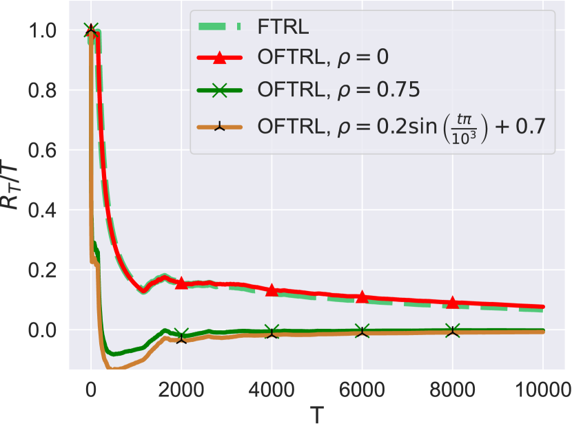
(a) OFTRL-Cache

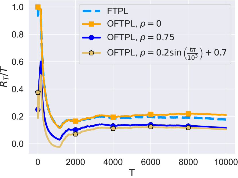
(b) OFTPL-Cache

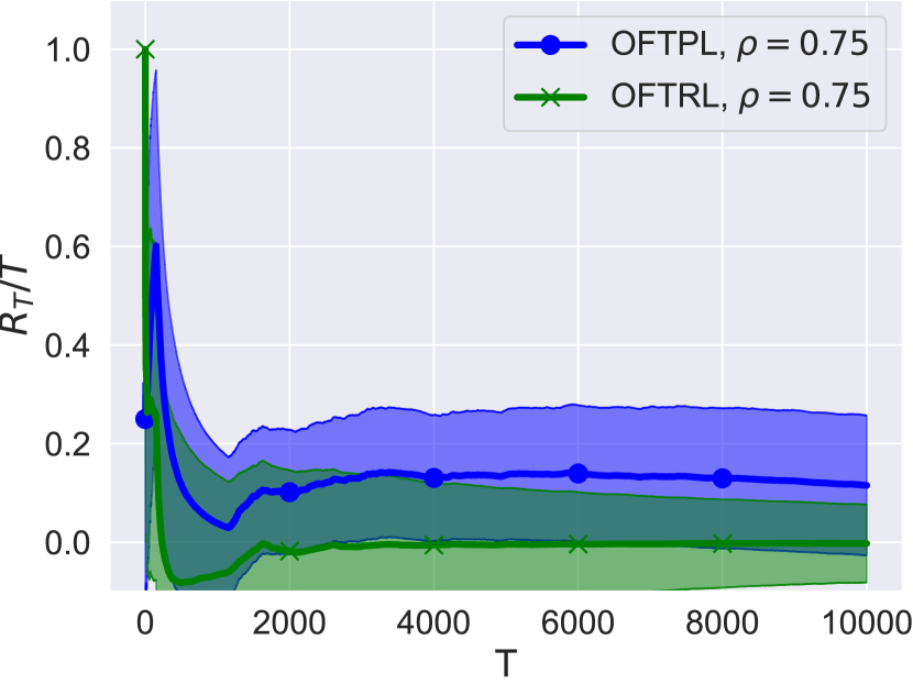
(c) OFTRL/OFTPL, $\rho\!=\!0.75$

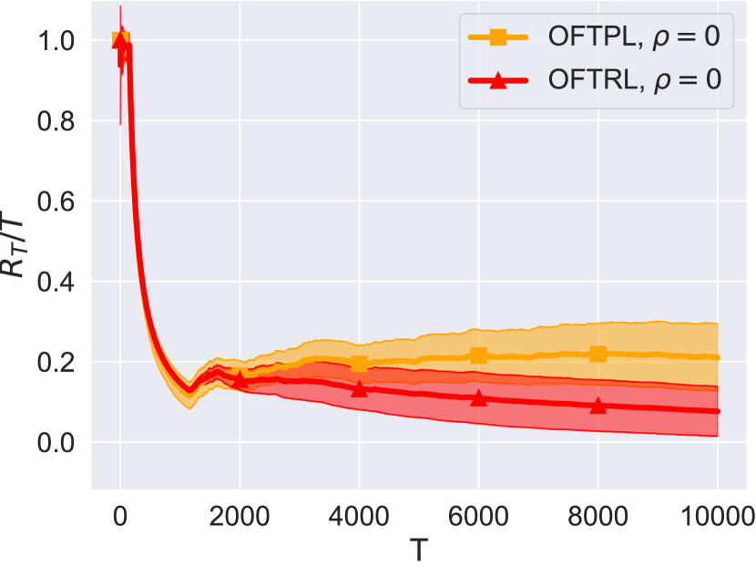
(d) OFTRL/OFTPL, $\rho\!=\!0$

Figure 2. Comparison of $R_{T}/T$ for equal-sized files in a single cache and different policies: (a) OFTRL-Cache vs. FTRL/OGD; (b) OFTPL-Cache vs. FTPL (Bhattacharjee et al., 2020); (c) OFTRL-Cache vs. OFTPL-Cache for good predictions and in (d) for worst-case predictions. In (c), (d) we plot the $0.95$-confidence interval ($8$ runs).

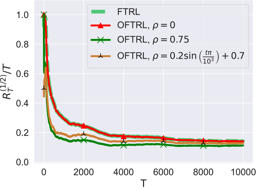
(a) OFTRL-UneqCache

(b) OFTPL-UneqCache

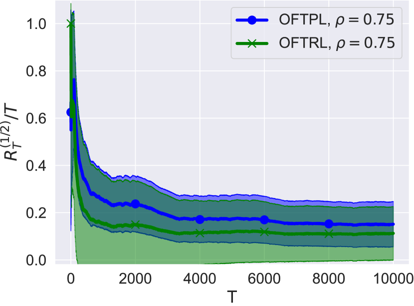
(c) OFTRL/OFTPL, $\rho\!=\!0.75$

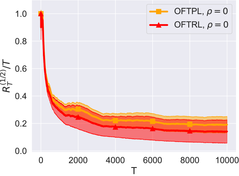
(d) OFTRL/OFTPL, $\rho\!=\!0$

Figure 3. Comparing $R_{T}^{(\nicefrac{{1}}{{2}})}/T$ for unequal-sized files, single cache. (a) OFTRL-UneqCache vs. FTRL/OGD; (b) OFTPL-UneqCache vs. FTPL (Bhattacharjee et al., 2020); (c)-(d) OFTRL-UneqCache vs. OFTPL-UneqCache for good (bad) predictions.

Fig. 2 shows the average regret (hit-rate gap to the optimal) growth with time for FTPL (Bhattacharjee et al., 2020), FTRL (Paschos et al., 2020a), and their proposed optimistic counterparts. We experiment with $\rho=0$, and $\rho=0.75$. If, e.g., the request predictions were based on recommendations, these reflect the cases where the users do not follow the recommendations ($\rho=0$), or actually request the recommended movie/file with probability $75\%$, ($\rho=0.75$). In addition, we experiment with a sinusoidal $\rho$, which varies between $\rho=0.5$ and $\rho=0.9$, with a period of $10^{3}$ slots. We observe that optimism accelerates and improves learning the best files to cache, reaching an average improvement of $104\%$ (for OFTRL) and $37.1\%$ (for OFTPL) when $\rho=0.75$, compared to their ”vanilla” counterparts (no predictions). Moreover, the performance degradation due to inaccurate predictions is almost negligible: $\leq 8.3\%$ for OFTRL and $\leq 6.6\%$ for OFTPL. We also plot the $0.95$-confidence interval of $R_{T}$ in Figures 2(c) and 2(d), where we note the more condensed distribution for OFTRL: $44.3\%$ and $26.1\%$ tighter at $t=10k$ when $\rho=0.75,\rho=0$, respectively. This is because the distribution ($\{\hat{x}_{t}\}_{T}$ iterates in OFTRL) becomes more concentrated with time; an argument that is not directly applicable to OFTPL, where the randomness is due to solving a perturbed linear program. In Fig. 3 we evaluate the algorithms for the unequal sizes case and plot the $\nicefrac{{1}}{{2}}$-regret. We observe the same pattern of negligible performance degradation when $\rho=0$, while $\rho=0.75$ enables an improvement of $35\%$ (for OFTRL) and $18.8\%$ (for OFTPL). We kindly refer the reader to the appendix for additional experiments for the experts-caching algorithm, the bipartite caching problem, and with probabilistic predictions of varying qualities.

10. Conclusions and Future Work

In this paper, we presented several provably optimal algorithms that exploit predictions of unknown quality to improve the regret bounds for important variants of the discrete caching problem, while maintaining worst-case guarantees. The tackled problems are general (e.g., the Knapsack problem) and extend beyond caching; and hence the corresponding proposed optimistic algorithms can be applied to other similar problems. Our approach was based on the unified view of FTRL and FTPL algorithms as smoothing operations, where we proposed to make such smoothing adaptive to the predictions’ accuracy. This allowed us to obtain a regret that interpolates between $0$ and $O(\sqrt{T})$.

This work also paves the road for several promising extensions. Given that eviction-only policies such as LFU or LRU have provably linear worst-case regret (Bhattacharjee et al., 2020), we studied policies that can dynamically prefetch files. Thus, balancing the cache hits with prefetching costs remains to be tackled. Moreover, we note that static regret algorithms, like ours, can be used as a subroutine in algorithms with stronger benchmarks, such as the $\Phi$-regret (Gordon et al., 2008) and the minimum regret over all Finite-State-Predictors (Joshi and Sinha, 2022), and extending the study towards such more-refined benchmarks is certainly interesting. Finally, considering unequal routing utility (e.g., link-capacitated model (Poularakis et al., 2014)) and unequal-sized files for the bipartite network model remains an open question (Mukhopadhyay et al., 2022).

Appendix A Appendix

A.1. Comparative Summary with Related Work

Table 1 shows the performance and complexity trade-offs for the presented algorithms, and compares them to recent studies of discrete no-regret caching in the literature. The best case refers to the situation where the request predictions are perfect $\tilde{\theta}_{t}=\theta_{t},\forall t$. The worst case refers to the situation where predictions are furthest from the truth $\tilde{\theta}_{t}=\arg\max_{\theta}\|\theta-\theta_{t}\|,\forall t$. The previous studies have the best and worst case columns merged as they do not utilize predictions. Furthermore, the works of (Bhattacharjee et al., 2020) and (Si Salem et al., 2021a) assume and utilize knowledge of the time horizon $T$ ( (Li et al., 2021) uses the standard doubling trick) and use the Lipschitz constant for the gradient (i.e., request) vector. Thus, they are not classified as performing Adaptive Learning (Adap. Learn.) as defined by (McMahan, 2017), which argues about the advantages of adaptive algorithms of the sort presented here. While the authors in (Bhattacharjee et al., 2020) discuss the bipartite model, their simpler linear elastic model of utility is different than the one considered here (see (Bhattacharjee et al., 2020, Sec. 3.2)). Hence, we compare to their single cache result. Finally, for algorithm $5$, we make explicit the dependence on weights regret $R_{T}^{(w)}$, although it is still $R_{T}^{(w)}\leq O(\sqrt{T})$ to clarify the cause of inferior performance of the experts-based optimism in the worst case compared to adaptive smoothing, which even appears in the simulations.

Table 1. Online discrete caching policies with adversarial no regret guarantees: a summary of the contributions and comparison with literature. For the constant $\alpha$, recall that $\alpha=1$ indicates the regular regret. Otherwise, we have $\alpha$-approximate regret (see equation (36)).

Alg.	Model and Conditions	Guarantees ($R^{(\alpha)}_{T}\leq$ )		Comput. Complex.	Approx. Const. $\alpha$	Adap. Learn.
		Best case	Worst case
1	$\bullet$ Single cache $\bullet$ Predictions	$0$	$O(\sqrt{T})$	$O(N^{2})$	$1$	✓
2	$\bullet$ Single cache $\bullet$ Predictions	0	$O(\textit{poly-log}(N)\sqrt{T})$	$O(N)$	$1$	✓
3	$\bullet$ Single cache $\bullet$ Predictions $\bullet$ Unequal sizes	$0$	$O(\sqrt{T})$	$O(N^{2})$	$\nicefrac{{1}}{{2}}$	✓
4	$\bullet$ Single cache $\bullet$ Predictions $\bullet$ Unequal sizes	0	$O(\textit{poly-log}(N)\sqrt{T})$	$O(N)$	$\nicefrac{{1}}{{2}}$	✓
5	$\bullet$ Bipartite Network $\bullet$ Predictions	0	$O(\sqrt{T})$	$O(N^{2})$	$1-\nicefrac{{1}}{{e}}$	✓
6	$\bullet$ Single Cache $\bullet$ Predictions	$b<0$	$R_{T}^{(w)}+O(\sqrt{T})$	$O(N)$	$1$	✓
(Bhattacharjee et al., 2020)	$\bullet$ Single cache	$O(\textit{poly-log}(N)\sqrt{T})$		$O(N)$	$1$	–
(Si Salem et al., 2021a)	$\bullet$ Single cache	$O\left(\sqrt{T}\right)$		$O(N)$	$1$	–
(Paria and Sinha, 2021)	$\bullet$ Bipartite network	$O(\textit{poly-log}(N)\sqrt{T})$		$O(N)$	$1-\nicefrac{{1}}{{e}}$	✓
(Li et al., 2021)	$\bullet$ General network	$O(\textit{poly-log}(N)\sqrt{T})$		$O(N)$	$1-\nicefrac{{1}}{{e}}$	–

A.2. Madow’s Sampling Algorithm

Algorithm 7 describes how we obtain an integral caching vector from the continuous one. We start by sampling a uniform scalar and then loop for $C$ iterations, including in our gradually-built set exactly one item per iteration. Hence we ensure the resulting set satisfies the capacity constraint. During an iteration, we include an item if its probability (continuous variable) falls in a carefully designed range: $[\pi_{j-1},\pi_{j}]$. Hence, each item is included with probability $\pi_{j-1}-\pi_{j}=\hat{x}_{i}$. We refer the reader to (Madow, 1949) for futher details.

1 Input: $\hat{x}\in[0,1]^{N},\sum x_{i\in\mathcal{N}}\leq C$.

2Output: Random set $S$, s.t $|S|=C$ and $\Pr(i\in S)=x_{i}$

3Sample a uniformly random scalar $U\in[0,1]$

4 Define the cumulative probabilities $\pi_{0}=0,\quad\pi_{i}=\pi_{i-1}+\hat{x}_{i},\quad\forall\ 1\leq i\leq N$

5for  $i=0,1,\ldots,C$  do

      6 $S\leftarrow S\cup\left\{j:\pi_{j-1}\leq U+i<\pi_{j}\right\}$

end for

7return $S$

Algorithm 7 Madow’s Sampling (MadowSample)

A.3. Dependent Rounding Algorithm ($DepRound$)

The dependent rounding algorithm operates sequentially. At each iteration, it picks two continuous variables and transfers at least one of them into an integer (through the if statements in lines $4$ to $8$), while adjusting the other one (lines $9$ to $12$). Hence, we ensure that when the algorithm terminates, only one item is still fractional. The properties of the resulting vector listed in Lemma 3 are proved in (Byrka et al., 2017, Lem. 2.1).

1 Input: $a\in[0,1]^{N},s\in R_{+}^{N}$.

2Output: $b$ satisfying points in lemma-3.

3 while $a$ contains two or more fractional elements do

      4 Denote the two left most fracitonal elements $a_{i}$ and $a_{j}$.

      5 if $0\leq s_{i}\ a_{i}+s_{j}\ a_{j}\leq\min\{a_{i},a_{j}\}$ then

             Set $b_{i}=0$ with probability $\nicefrac{{s_{j}a_{j}}}{{s_{i}a_{i}+s_{j}a_{j}}}$. With the remaining probability set $b_{j}=0$

       end if

      6if $a_{i}\leq s_{i}\ a_{i}+s_{j}\ a_{j}\leq a_{j}$ then

             Set $a_{i}=1$ with probability ${a_{i}}$. With the remaining probability set $a_{i}=0$

       end if

      7if $a_{j}\leq s_{i}\ a_{i}+s_{j}\ a_{j}\leq a_{i}$ then

             Set $a_{j}=1$ with probability ${a_{j}}$. With the remaining probability set $a_{j}=0$

       end if

      8if $\max\{a_{i},a_{j}\}\leq s_{i}\ a_{i}+s_{j}\ a_{j}\leq a_{i}+a_{j}$ then

             Set $b_{i}=1$ with probability $\nicefrac{{s_{j}(1-a_{j})}}{{(s_{i}(1-a_{i}))+(s_{j}(1-a_{j}))}}$. With the remaining set $b_{j}=1$

       end if

      9if $b_{i}=0$ set $b_{j}=\nicefrac{{s_{i}}}{{s_{j}}}\ a_{i}+a_{j}$

      10 if $b_{i}=1$ set $b_{j}=a_{j}-\nicefrac{{s_{i}}}{{s_{j}}}\ (1-a_{i})$

      11 if $b_{j}=0$ set $b_{i}=a_{i}+\nicefrac{{s_{j}}}{{s_{i}}}\ a_{j}$

      12 if $b_{j}=1$ set $b_{i}=a_{i}-\nicefrac{{s_{j}}}{{s_{i}}}\ (1-a_{j})$

      

end while

return $b$

Algorithm 8 Dependent Rounding (DepRound)

A.4. Proof of Theorem 2

Proof.

Since ${y_{ti}}\in\{0,1\}\ \forall t,i$, and the sampling in line $8$ is uniform, we get $\mathop{\mathbb{E}}\left[{y_{ti}}\right]=\frac{1}{2}$. Hence

(43) $$\mathop{\mathbb{E}}\left[{y_{ti}}\right]\geq\frac{1}{2}\hat{y}_{ti}.$$

where we have used that $\hat{y}_{t}\in[0,1]^{N}$. Now, from the definition of $\nicefrac{{1}}{{2}}$-Regret we have:

(44) $$R_{T}^{(\nicefrac{{1}}{{2}})} =\frac{1}{2}\sum_{t=1}^{T}\langle\theta_{t},y^{\star}\rangle-\mathbb{E}\left[\sum_{t=1}^{T}\langle\theta_{t},{y}_{t}\rangle\right]\stackrel{{\scriptstyle(a)}}{{\leq}}\frac{1}{2}\left(\sum_{t=1}^{T}\langle\theta_{t},y^{\star}\rangle-\sum_{t=1}^{T}\langle\theta_{t},\hat{y}_{t}\rangle\right)$$

(45) $$\stackrel{{\scriptstyle(b)}}{{=}}1.84\sqrt{C}\left(\ln\frac{Ne}{C}\right)^{1/4}\sqrt{\sum_{t=1}^{T}\|\theta_{t}-\tilde{\theta}_{t}\|_{1}^{2}}.$$

where inequality $(a)$ follows from the $\nicefrac{{1}}{{2}}$-approximation property of the randomized rounding algorithm (43); and $(b)$ follows from the result of Theorem 1.

∎

A.5. Proof of Theorem 4

First, we show that the $\nicefrac{{1}}{{2}}$-point-wise approximation holds for $\{x_{t}\}_{t}$. Then, we re-use the result of Theorem 1. In detail, by Lemma 3, the DepRound subroutine returns $\bar{x}_{t}$ such that $\mathop{\mathbb{E}}\left[{\bar{x}_{t}}\right]=\hat{x}_{t}$. Then, by the same argument about uniform sampling in the proof of Theorem 2, we have that $\mathop{\mathbb{E}}\left[{x_{t}}\right]\geq\frac{1}{2}\bar{x}_{t}$, where $x_{t}\in\mathcal{X}_{s}$. We recover our $\nicefrac{{1}}{{2}}$-approximation guarantee for OFTRL iterates $\{x_{t}\}_{t}$:

(46) $$\mathop{\mathbb{E}}\left[{x_{t}}\right]\geq\frac{1}{2}\hat{x}_{t}.$$

By the definition of $\nicefrac{{1}}{{2}}$-regret guarantee, we have

$$\!\!\!R_{T}^{(\nicefrac{{1}}{{2}})} =\frac{1}{2}\sum_{t=1}^{T}\langle\theta_{t},\hat{x}^{\star}\rangle-\mathbb{E}\left[\sum_{t=1}^{T}\langle\theta_{t},{x}_{t}\rangle\right]\stackrel{{\scriptstyle(a)}}{{\leq}}\frac{1}{2}\big{(}\sum_{t=1}^{T}\langle\theta_{t},\hat{x}^{\star}\rangle-\sum_{t=1}^{T}\langle\theta_{t},\hat{x}_{t}\rangle\big{)}\stackrel{{\scriptstyle(b)}}{{=}}\sqrt{C}\sqrt{\sum_{t=1}^{T}\|\theta_{t}-\tilde{\theta}_{t}\|_{2}^{2}}.$$

where inequality $(a)$ follows from the $\nicefrac{{1}}{{2}}$-approximation property of the randomized rounding algorithm (46); and $(b)$ follows from the result of Theorem 1. Although that theorem states the bound for the regret of the integral decisions $\{x_{t}\}_{t}$, we have seen in its proof that the bound is essentially the same for the continuous actions.

A.6. Proof of Theorem 1

We start from the result of (Mhaisen et al., 2022a, Thm. 1) (or its earlier version from (Mhaisen et al., 2022b)), which provides guarantees for the regret of the continuous variables $\hat{x}$. For the moment, assume that we have the following point-wise approximation for the decision variables $\mathbb{E}[\hat{k}]=k$, $\mathop{\mathbb{E}}\left[{\hat{u}}\right]\geq(1-\nicefrac{{1}}{{e}})u$, and that the capacity constraints are respected. Then, due to the linearity of the objective function $f_{t}(\cdot)$, we get that our $\alpha$-regret (with $\alpha=1-\nicefrac{{1}}{{e}}$) is:

$$R_{T}^{(1-\nicefrac{{1}}{{e}})} =(1-\frac{1}{e})\sum_{t=1}^{T}\langle\theta_{t},\hat{x}^{\star}\rangle-\mathbb{E}\sum_{t=1}^{T}\langle\theta_{t},{x}_{t}\rangle\stackrel{{\scriptstyle(a)}}{{\leq}}1-\frac{1}{e}\big{(}\sum_{t=1}^{T}\langle\theta_{t},\hat{x}^{\star}\rangle-\sum_{t=1}^{T}\langle\theta_{t},\hat{x}_{t}\rangle\big{)}$$

$$\stackrel{{\scriptstyle(b)}}{{=}}(2-\frac{2}{e})\sqrt{1+JC}\sqrt{\sum_{t=1}^{T}\|\theta_{t}-\tilde{\theta}_{t}\|_{2}^{2}}.$$

where inequality $(a)$ follows from the $(1-\nicefrac{{1}}{{e}})$-approximation property of the randomized rounding algorithm; and $(b)$ follows from the result of Theorem (Mhaisen et al., 2022a, Thm. 1).

Now, to show that $\mathbb{E}[\hat{k}]=k$, we follow the same argument in the proof of Theorem 1. Namely, due to Madow’s sampling, each file is included with probability $\hat{k}$, and at most $C_{j}$ files are included at each cache. Hence, $\mathop{\mathbb{E}}\left[{k_{nj}}\right]=\hat{k}_{nj},\forall{n,j}$. Regarding the point-wise approximation for $u$, we define the set $\mathcal{J}^{i}$ of caches connected to user $i$:

$$\mathcal{J}^{i}=\left\{j\in\mathcal{J}\big{|}\ d_{ij}=1\right\}.$$

Then, we have

(47) $$\mathop{\mathbb{E}}\left[{u_{nij}}\right] \stackrel{{\scriptstyle(a)}}{{=}}\Pr[u_{nij}=1]\stackrel{{\scriptstyle(b)}}{{=}}\Pr[\vee_{j\in\mathcal{J}^{i}}k_{nj}=1]\stackrel{{\scriptstyle(c)}}{{=}}1-\prod_{j\in\mathcal{J}^{i}}\big{(}1-\hat{k}_{nj}\big{)}$$

$$\stackrel{{\scriptstyle(d)}}{{\geq}}1-e^{-\sum_{j\in\mathcal{J}^{i}}\hat{k}_{nj}}\stackrel{{\scriptstyle(e)}}{{\geq}}1-e^{-\hat{u}_{nij}}\stackrel{{\scriptstyle(f)}}{{\geq}}\left(1-\frac{1}{e}\right)\hat{u}_{nij}.$$

Where in the above chain of inequalities, $(a)$ follows from $u_{nij}$ being binary variable; $(b)$ by the construction of the algorithm (step $8$); and $(c)$ from the independent rounding for each cache. Also, inequality $(d)$ follows from from $e^{x}\geq 1+x,\forall{x}\in\mathbb{R}$; $(e)$ from the relaxed version of the caching/routing constraint of $\mathbb{P}_{2}$, and finally $(f)$ from the concavity of $1-e^{-x}$ and the domain of $\hat{u}_{nij}$ being restricted to $[0,1]$.

A.7. Additional Simulations

A.7.1. Probabilistic Predictions

Let us first demonstrate, with a simple example, that using probabilistic predictions is beneficial for the performance of optimistic algorithms. The regret bound of the proposed algorithms depend on the terms $\|\theta_{t}-\tilde{\theta}_{t}\|$, $\forall t$. Now, consider a prediction $\tilde{\theta}_{t}$ that places $\epsilon$ probability mass on the correct file, and the remaining uniformly over the rest of the files in the library. Then, we get:

$$\|\theta_{t}-\tilde{\theta}_{t}\|_{2}\approx 1-\epsilon,\quad\text{since}\quad\frac{(1-\epsilon)^{2}}{(N-1)}\approx 0,$$

compared to a mis-prediction (or, mistaken) one-hot $\tilde{\theta}_{t}$ which will have $\|\theta_{t}-\tilde{\theta}_{t}\|_{2}=\sqrt{2}$. Using the $\ell_{1}$ norm, a one-hot mistake costs $2$ compared to $2-2\epsilon$ for the probabilistic one. We stress again that all the results presented in this work hold both for probabilistic and for deterministic predictions. The former can be taken directly from the output of a forecasting model, while one can create the latter by simply using the highest-probability request.

We continue by presenting experimental results for a probabilistic prediction model with varying accuracy. In detail, in Fig. 4 we measure the regret of the proposed OFTRL and OFTPL policies after $5k$ time steps (i.e., file request) using the well-known YouTube request trace (Zink et al., 2009) with $N=10^{4}$ and $C=150$. $R_{5k}$ is measured using prediction vectors with varying density that is placed on the file to be requested. Namely, if at step $t$, the requested file is $n$, we feed the optimistic algorithms with a prediction vector:

$$\tilde{\theta}\quad\text{with:}\quad\tilde{\theta}^{t}_{n}=\zeta\quad\text{and}\quad\tilde{\theta}^{t}_{n^{\prime}}=(1-\zeta)/(N-1),\ \forall n^{\prime}\neq n.$$

That is, the prediction vector has $\zeta$ probability placed on the file to be requested, and the remaining ($1-\zeta$) uniformly distributed across the remaining files. We note that when the prediction vector is almost uniform (i.e., $\tilde{\theta}$ contains no useful information), the optimistic versions nearly match the non optimistic ones.

We can see that at $\zeta=0.1$, both OFTRL and OFTPL already start outperforming their non-optimistic counterparts, by $9.8\%$ and $1.4\%$, respectively. Also, they outperform the best-in-hindsight benchmark $x^{\star}$ when the accuracy becomes reasonably high ($\zeta\geq 0.8$). Lastly, we see that OFTRL has a performance advantage of up to $59.6\%$ compared to OFTPL, when fed the same predictions, at the expense of its additional computation complexity.

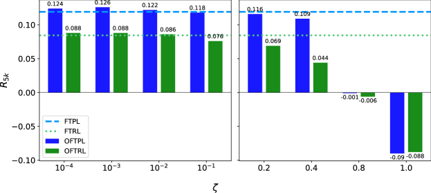
Figure 4. Regret with varying probability mass placed on the correct file in the prediction vector.

A.7.2. Algorithms 5 and 6

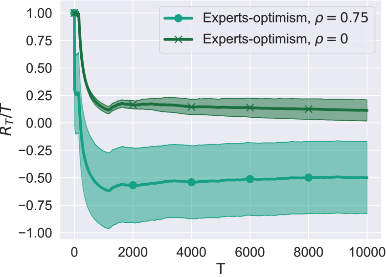
Figure 5. Average regret of experts-based optimism.

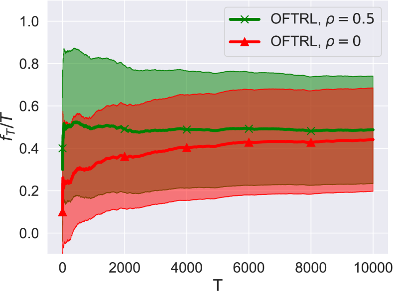
Figure 6. Average OFTRL hit-rate for cache network.

Fig. 5 plots the regret for the expert-based Algorithm 6. Note that the $R_{T}$ can reach negative values, i.e., outperform better the benchmark, when $\rho=0.5$. This is aligned with the bound in (42) and hints to the fact that stronger benchmarks can be used for this algorithm. However, it performs worse than the regularization-based optimism in the case where $\rho=0$, achieving regret $R_{T}=0.113$ at time $T=10k$ compared to $R_{T}=0.075$ (OFTRL). Lastly, the bipartite utility is shown in Fig. 6, the hit-ratio of OFTRL is approximately $0.49$ when $\rho=0.5$. Expectantly, the performance drops when $\rho=0$, but steadily increases from $0.30$ at $T=500$, to $0.44$ at $T=10k$.