Probabilistic Variational Causal Effect as A new Theory for Causal Reasoning

Abstract.

In this paper, we introduce a new causal framework capable of dealing with probabilistic and non-probabilistic problems. Indeed, we provide a direct causal effect formula called Probabilistic vAriational Causal Effect (PACE) and its variations satisfying some ideas and postulates. Our formula of causal effect uses the idea of the total variation of a function integrated with probability theory. The probabilistic part is the natural availability of changing an exposure values given some variables. These variables interfere with the effect of the exposure on a given outcome. PACE has a parameter $d$ determining the degree of considering the natural availability of changing the exposure values. The lower values of $d$ refer to the scenarios for which rare cases are important. In contrast, with the higher values of $d$, our framework deals with the problems that are in nature probabilistic. Hence, instead of a single value for causal effect, we provide a causal effect vector by discretizing $d$. Further, we introduce the positive and negative PACE to measure the positive and the negative causal changes in the outcome while changing the exposure values. Furthermore, we provide an identifiability criterion for PACE to deal with observational studies. We also address the problem of computing counterfactuals in causal reasoning. We compare our framework to the Pearl, the mutual information, the conditional mutual information, and the Janzing et al. frameworks by investigating several examples.

1. Introduction

As human beings as soon as we wake up, consciously or unconsciously we try to figure out what is wrong. For instance, why do I feel depressed. Is that because I could not sleep last night as a result of health issues or I ate too much and that upset my stomach. Causal reasoning is used in every aspect of our life, for instance in healthcare, industry, and education.

The most notable frameworks in causal inference are the Neyman-Rubin framework ([18], [38]) and the Pearl framework ([32]). Roughly speaking, the Neyman-Rubin framework is based on the idea of potential outcomes. For instance, for an individual (or unit), a binary treatment $T$ results in two potential outcomes that cannot be simultaneously observed: 1) the outcome when $T=0$, and 2) the outcome when $T=1$. The potential outcome which is not observable is called the counterfactual outcome. The difference between these potential outcomes is defined as the individual causal effect of $T$ on the outcome variable. Next, to aggregate the effects for the whole population, different ideas and formulas could be used (e.g., the expected value of the individual causal effects). To measure the direct causal effect of $T$ on the outcome variable, formulas such as controlled direct effect and natural direct effect are used. Missing data due to counterfactual outcomes is the fundamental problem of the Neyman-Rubin framework. To deal with this issue, identifiability criteria are used (for more information on the Neyman-Rubin framework, see Section 3.1). The Pearl framework is more general than the Neyman-Rubin framework, and it is based on the idea of intervention in graphical causal models. Practically, the intervention $T=t$ for an individual has the same meaning as the potential outcome with respect to $T=t$. However, Pearl provides graphical causal models by using Baysian networks to investigate causality (see Section 3.2). Among the other causal frameworks, the information theoretic frameworks ([19]) including the Janzing et al., the mutual information, and the conditional mutual information frameworks are notable (see Section 3.3). These information theoretic frameworks have specific applications and fail to correctly answer the causal questions in which rare cases are important.

The main idea of our causal framework is the natural availability of changing of the exposure/treatment variable. For instance, assume that we are going to measure the direct causal effect of the presence of a rare natural noise $N$ on the quality $Q$ of a certain type of photo. Also, assume that $Q=g(N,\bm{\mathrm{O}})$, where $\bm{\mathrm{O}}$ denotes all other variables directly affecting $Q$. Then, in real world data $\mathbb{P}(N=1|\bm{\mathrm{o}})$ is a very low value due to the rarity of $N$. Hence, this noise affects a photo rarely. Thus, we believe that $\mathbb{P}(N=1|\bm{\mathrm{o}})$ should affect the direct causal effect of $N$ on $Q$, since low values for $\mathbb{P}(N=1|\bm{\mathrm{o}})$ means lower noisy photos. Therefore, our sense of causality is built by an integration of the interventions $N=0$ and $N=1$, and the natural availability of changing $N=0$ to $N=1$ while keeping $\bm{\mathrm{O}}=\bm{\mathrm{o}}$ constant. However, if we consider the Pearl framework, the interventions $N=0$ and $N=1$ do not have anything to do with $\mathbb{P}(N=1|\bm{\mathrm{o}})$ (see Section 4.10). Consequently, we believe that there is an essential need for a generic causal framework capable of answering different types of causal questions.

Let $X$ be a random variable that we are looking for its direct causal effect on the outcome variable $Y$. Also, let $Y=g(X,\bm{\mathrm{Z}})$, where $\bm{\mathrm{Z}}$ is the random vector consisting of all other variables directly affecting $Y$. In general, we assume that the above equation is the last equation of an structural equation model (SEM) (see Section 2.5). In this paper, we introduce a new generic causal framework capable of answering a wide variety of causal questions. Indeed, we provide a direct causal effect formula called probabilistic variational causal effect (PACE) satisfying some ideas and postulates (see Section 4.1). PACE is defined as an integration of the total variation of a function (see Section 2.1) and probability theory. The probabilistic part of PACE of $X$ on $Y$ is the natural availability of changing $X$ values given $\bm{\mathrm{Z}}$. PACE has a parameter $d$ determining the degree of considering the natural availability of changing $X$ values. The lower values of $d$ refer to the scenarios for which rare cases are important. In contrast, with the higher values of $d$, our framework deals with the problems that are in nature probabilistic. Hence, instead of a single value for causal effect, we provide a causal effect vector by discretizing $d$. Also, we define some variations of PACE and investigate their properties (see Section 4.4). Further, we provide the positive and the negative PACEs to measure the positive and the negative causal changes of $Y$ by changing $X$ values while keeping $\bm{\mathrm{Z}}$ constant. In fact, if we change the value of $X$ from $x$ to $x^{\prime}$ ($x<x^{\prime}$) while keeping $\bm{\mathrm{Z}}$ constant, then for the positive change of $Y$, we say that we have a positive direct causal effect on $Y$. Similarly, the negative direct causal effect is defined. Furthermore, to deal with observational studies, we provide an identifiability criterion for PACE (see Section 4.9). We also explain how PACE could be used for calculating the causal effect of a random variable $W$ on $Y$ along some paths from $W$ to $Y$. To do so, the main idea is to replace the mediators by their parents and update the SEM (see Section 4.7).

Now, we explain the organization of the paper. In Section 2, we provide some basic knowledge including the total variation of a function and its applications, the philosophical and the scientific approaches for causality, the information theoretic concepts required in this paper, the directed acyclic graphs, and structural equation models. Section 3 is devoted to the related works. In this section, we briefly explain the aforementioned causal frameworks by investigating an example. In Section 4, we explain our framework by providing the PACE formula and some of its properties. Further, we provide some variations of PACE called PEACE, SPACE, and APACE, and investigate their properties and their relationships. We go further and give matrix representations for PACE and its variations, and then we provide an idea to define more general variational direct effect formulas. Furthermore, the positive and the negative PACEs are introduced and discussed. Finally, we study the identifiability of PACE and its variations, the indirect causes of an outcome variable, and we compare our framework to the Pearl framework. Next, in Section 5, we investigate three different examples showing the generalization capacity of PACE compared to the above frameworks. Further, in these examples, we address the problem of computing counterfactuals in causal reasoning by the same procedure explained in [14].

In this paper, all the random variables discussed are finite unless otherwise stated.

2. Preliminaries

2.1. Total Variation

In this subsection, we briefly explain the total variation formula for functions of one and several variables. Further, we mention the importance of the total variation of a function in different branches of science.

2.1.1. Total Variation of a Function of one Variable

Let $f:[a,b]\to\mathbb{R}$ be a function. A partition for the interval $[a,b]$ is a an ordered set $P=\{a=x_{0}^{(P)}<x_{1}^{(P)}<\cdots<x_{n_{P}-1}^{(P)}<x_{n_{P}}^{(P)}=b\}$. Denote the set of all partitions of $[a,b]$ by $\mathcal{P}([a,b])$. Then, the total variation of $f$ is defined as follows:

$$\mathcal{V}(f):=\sup_{P\in\mathcal{P}([a,b])}\sum_{i=1}^{n_{P}}|f(x_{i}^{(P)})-f(x_{i-1}^{(P)})|.$$

To the best of our knowledge, the idea of the total variation for the first time was discussed in [20]. It is well-known that if $f$ is continuously differentiable, then $\mathcal{V}(f)=\int_{a}^{b}|f^{\prime}(t)|\,\mathrm{d}t$, and hence $\mathcal{V}(f)$ is the arc length of $f$ as a 1-dimensional curve in $\mathbb{R}$. This arc length could be thought of as the distance that a particle travels on a straight line in the time interval $[a,b]$ with the position vector $f(t)$ for $t\in[a,b]$.

2.1.2. Total Variation of a Function of Several Variables

The total variation has been generalized for multivariate real valued functions in several ways (for instance, see [2], [5], [6], [11], [15], [33], [43] and [45]). The following generalization of the total variation for functions of several variables is often used in modern literature. We also consider it in the sequel (see [10, Section 5.1]). Let $\Omega$ be an open subset of $\mathbb{R}^{n}$ and $f:\Omega\to\mathbb{R}$ be (Riemann) integrable. Then, the total variation of $f$ on $\Omega$ is defined as follows:

$$\mathcal{V}(f)=\sup\left\{\int_{\Omega}f(x)\mathrm{div}(\phi)(x)\,\mathrm{d}x:\phi\in\mathrm{C}_{c}^{\infty}(\Omega,\mathbb{R}^{n}),\;\lVert\phi\rVert_{\infty}\leq 1\right\},$$

where $\mathrm{C}_{c}^{\infty}(\Omega,\mathbb{R}^{n})$ is the set of all smooth functions from $\Omega$ to $\mathbb{R}^{n}$ whose supports are compact, $\lVert\,\cdot\,\rVert_{\infty}$ denotes the $L^{\infty}$-norm, and $\mathrm{div}(\phi)$ denotes the divergence of $\phi$. Under some ”good” assumptions, by the divergence theorem we have that:

$$\mathcal{V}(f)=\int_{\Omega}\left|\nabla f\right|(x)\,\mathrm{d}x,$$

where $\nabla f$ is the gradient of $f$.

For a generalization of the total variation formula for signed and complex measures in Measure Theory, see [41].

2.1.3. Functions with Bounded Total Variation and Their Importance

Note that the total variation of a function as above might be $\infty$. The space of functions of bounded total variation (or simply BV functions) on an open subset $\Omega$ of $\mathbb{R}^{n}$, denoted by $\mathrm{BV}(\Omega)$, is of interest of many mathematicians due to the following properties:

• $\mathrm{BV}(\Omega)$ is a Banach space (i.e., a normed space in which every Cauchy sequence converges).

• $\mathrm{BV}(\Omega)$ is a Banach algebra (i.e., a Banach space equipped with an associative multiplication operator compatible with the sum and the scalar product).

• Every $f\in\mathrm{BV}(\Omega)$ can be uniquely decomposed to $f=g-h$, where $g$ and $h$ are two bounded and increasing functions (see [37, Section 5.2]).

• The chain rule on $\mathrm{BV}(\Omega)$, which consider the generalized partial derivatives, is useful for physical models dealing with the lack of smoothness (see [46, Page 248]).

• The characteristic function of a set with finite measure whose boundary is measurable is a BV function. The aforementioned sets are called Caccioppoli sets and play a key role in the modern theory of perimeters (see [23]).

• Minimal surfaces (i.e., roughly speaking, the surfaces whose areas are minimal with respect to some constraints) are the graphs of BV functions (see [13]).

Further, for a BV function $f:[a,b]\to\mathbb{R}$, the following well-known properties are satisfied:

• $f$ is discontinuous in at most a countable set of points.

• One-sided limits (i.e., right and left limits) of $f$ exist.

• The derivative of $f$ exists almost everywhere (i.e., the set of points $t\in[a,b]$ for which $f^{\prime}(t)$ does not exist has the Lebesgue measure zero).

Furthermore, the followings make the BV functions more appealing to physicists, computer scientists, chemists, electrical and mechanical engineers:

• Due to the ability of BV functions to deal with discontinuities, solutions to problems in Physics, Mechanics, and Chemical Kinetics are mostly expressible by BV functions (see [47]).

• Total variation denoising in Signal Processing (see [12] and [39]).

2.1.4. Total Variation of a Sequence of Real Numbers

Let $\{x_{n}\}_{n=0}^{\infty}$ be a sequence of real numbers. Then, the total variation of this sequence is defined as follows (see [8, Chapter IV]):

$$\mathcal{V}\left(\{x_{n}\}_{n=1}^{\infty}\right)=\sum_{n=1}^{\infty}|x_{n}-x_{n-1}|.$$

The space of all BV sequences of real numbers could be turned into a Banach space isomorphic to $\ell_{1}$ (i.e., the space of all sequences $\{x_{n}\}_{n=0}^{\infty}$ of real numbers with $\sum_{n=0}^{\infty}|x_{n}|<\infty$ equipped with the following norm: $\lVert\{x_{n}\}_{n=0}^{\infty}\rVert=\sum_{n=0}^{\infty}|x_{n}|$).

2.1.5. Total Positive and Negative Variations

Let $r\in\mathbb{R}$. Define $r^{\bm{+}}:=\max\{r,0\}$ and $r^{\bm{-}}:=|r|-r^{\bm{+}}$. Then, the total positive variation of a function $f:[a,b]\to\mathbb{R}$ is defined as follows (see [20]):

$$\mathcal{V}(f)^{\bm{+}}:=\sup_{P\in\mathcal{P}([a,b])}\sum_{i=1}^{n_{P}}\left(f(x_{i}^{(P)})-f(x_{i-1}^{(P)})\right)^{\bm{+}}.$$

Similarly, the total negative variation of $f$ is defined as follows:

$$\mathcal{V}(f)^{\bm{-}}:=\sup_{P\in\mathcal{P}([a,b])}\sum_{i=1}^{n_{P}}\left(f(x_{i}^{(P)})-f(x_{i-1}^{(P)})\right)^{\bm{-}}.$$

One could easily see that $\mathcal{V}(f)=\mathcal{V}(f)^{\bm{+}}+\mathcal{V}(f)^{\bm{-}}$. The total positive and negative variations could be similarly defined for sequences of real numbers. In this case, one could see that $\mathcal{V}\left(\left\{x_{n}\right\}_{n=0}^{\infty}\right)=\mathcal{V}\left(\left\{x_{n}\right\}_{n=0}^{\infty}\right)^{\bm{+}}+\mathcal{V}\left(\left\{x_{n}\right\}_{n=0}^{\infty}\right)^{\bm{-}}$.

2.2. Causality, Causal Reasoning, and Causal Inference

Causality is a fundamental notion of science. For instance, in Physics, the notion of causality can be employed as a prior basis to construct space and time by using Minkowski Geometry and Special Theory of Relativity (see [24], [35], and [48]). Immanuel Kant believed that people have intrinsic assumptions about the causes and effects. However, David Hume believed that our minds are not able to recognize causes directly (see [25]). One’s understanding of ”causality” might change their worldview and consequently the way one prefers to live. For instance, the deterministic worldview states that the history of ”being” could be expressed as a cause-and-effect process. Many people who believe in this view find their worldview in contrast with ”free will”. The philosophical views of causality are as follows:

• Regularity (or Covariation): causes are followed by their effects regularly (see [1]).

• Probabilistic (or Dependency): causes change the probabilities of their effects (see [17]).

• Counterfactual: causal claims are stated as counterfactual conditionals such as “If $X$ had not happened, then $Y$ would not have happened” (see [26]).

• Mechanistic: $X$ and $Y$ are connected causally whenever there exists an underlying physical mechanism of the appropriate sort that connects $X$ and $Y$ to each other (see [27]).

• Manipulationist: If $X$ is a cause of $Y$ and one can manipulate $X$ in the ”right way”, then this should yield some changes in $Y$ (see [51]).

• Dynamics: causes are expressable by a pattern of forces (see [49] and [50]).

Some experts consider three types of cause as follows (for the first two types of cause one could see [30]):

• Necessary cause: ”$X$ is a necessary cause of $Y$” means that the occurrence of $Y$ necessarily implies the prior occurrence of $X$.

• Sufficient cause: ”$X$ is a sufficient cause of $Y$” means that the occurrence of $X$ implies the subsequent occurrence of $Y$.

• Contributory cause: ”$X$ is a contributory cause of $Y$” means that $X$ is one of the co-occurring events resulting in a certain effect on $Y$ (see [34]).

The process of discovering the relationship between causes and their effects is called causal reasoning, and it is mostly a philosophical phrase. In daily life, people often causally reason about different subjects. For instance, a common argumnet is that ”$X$ causes $Y$, and $Y$ causes $Z$. Therefore, $X$ causes $Z$”. Such arguments could be true or false or controversial. For instance, consider the following causal argument:

• My happiness caused Mike’s happiness, and Mike’s happiness caused Daniel’s sadness. Therefore, my happiness caused Daniel’s sadness.

The above argument seems to be weird and false unless a share of happiness that made Daniel sad had been caused by me. However, extra information might make the recent argument more reasonable. To see this, assume that Mike teases his friends when he is happy, and Daniel is Mike’s friend and becomes sad when someone teases him. Note that this argument is still controversial since we are not given any information about the levels of teasing and sadness and the relationship between them for Daniel. To make it more clear, assume that 1) Barcelona is my and Mike’s favorite team, while Daniel’s is Real Madrid, 2) last night Barcelona won the final match of UEFA Champions League against Real Madrid, 3) I watched the match, while Mike did not, and 4) I told Mike about our victory and he got happy, and he teased a little Daniel for the Real Madrid loss. Here, Daniel’s sadness might be caused by his favorite team losing the match not Mike’s teasing him.

A scientific approach to causal reasoning is called causal inference. More precisely, ”causal inference refers to an intellectual discipline that considers the assumptions, study designs, and estimation strategies that allow researchers to draw causal conclusions based on data”[16]. We define some common phrases in causal inference by using the above example. Indeed, the match result is a confounder due to its effect on both my happiness and Daniel’s sadness. Also, Mike’s happiness is a mediator due to its role in transiting the effect of my happiness to Daniel. Mike’s happiness and my happiness are an direct cause and an indirect cause of Daniel’s sadness, respectively. Now, let us encode the aforementioned example to a so-called causal graph. To do so, first we associate the following random variables to the example:

$$\begin{array}[]{ll}X=\left\{\begin{array}[]{ll}1,&\begin{array}[]{l}\text{I am happy, and }\\ \text{share my happiness}\\ \text{with Mike}\end{array}\\ 0,&\text{ otherwise}\end{array}\right.&Z=\left\{\begin{array}[]{ll}1,&\text{Mike is happy}\\ 0,&\text{Mike is not happy}\end{array}\right.\\ &\\ Y=\left\{\begin{array}[]{ll}1,&\text{Daniel is sad}\\ 0,&\text{Daniel is not sad}\end{array}\right.&W=\left\{\begin{array}[]{ll}1,&\text{Mike teases his friends}\\ 0,&\text{Mike does not tease his friends}\end{array}\right.\\ C=\left\{\begin{array}[]{ll}1,&\text{Barcelona wins}\\ 0,&\text{Real Madrid wins}\end{array}\right.&U_{X},U_{Y},U_{Z},\text{ and }U_{W}\text{ are {unobserved} variables}.\end{array}$$

Then, we have the causal graph shown in Figure 1. Causal graphs are usually considered as directed acyclic graphs (see Section 2.4)

Figure 1. An example of a causal graph (that is associated with the example discussed in Section 2.2)

To investigate causal problems, the following approaches are common:

• Experimental designs are conducted, when it is possible to keep some variables unchanged while manipulating a variable of interest (called the treatment variable) to see the changes in the outcome. Randomized controlled trials are examples that follow this approach by removing the dependency between the confounder and the treatment. This is done by randomly and (possibly) blindly assigning the treatment to the entire sample. Experimental designs are ideal to investigate causality, although the followings are some concerns about conducting this type of approach:

  • Ethical concerns: suppose that we are going to determine if someone smoking has a causal effect on her mood. Obviously, it is not ethical to randomly divide the sample into two groups and ask a group to smoke for a year and the other not.

  • Limitations of the influence: suppose that we are going to determine if the office working hours of a manufacturing company have a causal effect on the quality of the company’s products. Here, we need to have the authority or be allowed to interfere with the working hours of the company’s staff.

  • Possibility concerns: suppose that we are going to determine if the political system (e.g., capitalist or socialist) has a causal effect on the inner satisfaction of people. Here, apart from the difficulty and unethicality of exiling an individual from a capitalist political system to a socialist one (or vice versa), it is an overstatement to say it is possible to completely remove the effect of the capitalist (resp. socialist) political system on the individual.

  • Impracticality: suppose that we are going to determine if a treatment causes a rare side effect. Here, conducting an experimental design is impractical (e.g., economically) due to the need for a huge sample.

  • External validity issue: in experimental designs, individuals are most likely to be young, male, healthier, and treated according to the preferences of the guidelines (see [22]). Therefore, the obtained results might not be generalized to the entire population.

• Observational studies provide alternative approaches to investigate causality when the use of experimental designs is somehow problematic. To find out if a treatment has a causal effect on an outcome, the treatment and the control groups should be reasonably comparable or exchangeable (Randomized controlled trials satisfy this condition). Otherwise, different choices of treatment and control groups may lead us to different results of causality. For example, to causally investigate the effect of smoking on having lung cancer, gender is a confounder since women are more likely to have lung cancer and less likely to smoke. Hence, smokers in a random sample of the population are more likely to be men. This yields less chance of having lung cancer rather than a random sample equally including men and women smokers. We say that the condititional exchangeability assumption is satisfied when the exchangeability assumption is satisfied in any subpopulation (these subpopulations could be based on gender, socio-economic situations, etc). To satisfy exchangeability or conditional exchangeability assumptions, matching methods are usually suggested. Matching is used to reduce the bias of non-randomly assigning individuals to the treatment or the control groups due to the nature of observational studies. Propensity Score and Conditional Logistic Regression are two famous types of matching. For instance, the Propensity Score matching method consists of the following two steps: 1) calculating the probability of receiving the treatment in each subpopulation, called the propensity score (see [36]), and 2) two subpopulations with close propensity scores are paired in such a way that one receives the treatment and the other not. This follows that the conditional exchangeability condition is satisfied. However, Pearl has argued that Propensity Score matching on observed variables could increase the bias due to unobserved confounders (see [28]). On the contrary to the experimental designs, observational studies might suffer from a low internal validity . However, observational studies have the potential for high external validity.

• Quasi-experimental designs (natural experiments) also provide alternative approaches to investigate causality, when experimental designs cannot be completely conducted. In quasi-experimental designs, researchers might be able to control for or manipulate some variables but not all required variables. To the best of our knowledge, though many researchers consider quasi-experimental designs as types of observational studies, except for experimental designs, there is no clear categorization for the other scientific designs. Here, to deal with the non-randomness of the assignment mechanism, some different methods such as cut-off scores have been recommended.

We note that correlation is not causation. For instance, in the 1950’s compared to the 1930’s and 1940’s, the lung cancer rate dramatically increased. Most researchers concluded that this increase in rate is due to an increase in the smoking rate. However, the relationship between smoking and lung cancer could be only a correlation and not causation. In fact, there might be other reasons such as a confounder resulting in the aforementioned correlation (e.g., the increased rate of lung cancer could be the result of a better diagnosis, more polluted air due to particles such as exposure to lead, polycyclic aromatic hydrocarbons (PAHs), and other sources in the industry. Also, some specific genes could be confounders for both smoking and lung cancer). Therefore, statistics alone cannot answer causality questions. Roughly speaking, the procedure to convert a causality question into a statistical one on observed variables is called identifiability. This procedure needs some extra causal pre-assumptions. For instance, satisfying exchangeability and conditional exchangeability conditions (explained above) leads us to identifiability.

2.3. Some Information Theoretic Preliminaries

Let $p$ be the probability of observing an event $E$ in a random experiment. Then, $\log\left(\frac{1}{p}\right)$ is interpreted as the surprise value of $E$. Given the event $E$, for a lower value of $p$, we obtain a higher surprise value. Let $\Omega=\{\omega_{1},\ldots,\omega_{n}\}$ be the sample space of a random experiment with $\mathrm{Pr}=\{p_{1},\ldots,p_{n}\}$, where $P(\omega_{i})=p_{i}$ for $1\leq i\leq n$. Then, the expected value of surprise values for sample space points is called the entropy of the random experiment, denoted by $\mathbb{H}(\mathrm{Pr})$. Indeed, we have that

$$\mathbb{H}(\mathrm{Pr})=\sum_{i=1}^{n}p_{i}\log\left(\frac{1}{p_{i}}\right).$$

Let $X$ and $Y$ be two random variables whose sets of values are finite. If $\mathrm{Pr}_{X}$ be the set of all probability values of $X$, then $\mathbb{H}(\mathrm{Pr}_{X})$ is denoted by $\mathbb{H}(X)$. The entropies of the joint distribution of $X$ and $Y$, and the conditional distribution of $Y$ given $X=x$ are defined in a similar manner. Further, the conditional entropy $\mathbb{H}(Y|X)$ is defined as $\sum_{x}\mathbb{H}(Y|X=x)\mathbb{P}(X=x)$. One could see that if $Y$ is a function of $X$, then $\mathbb{H}(Y|X)=0$. Also, if $X$ and $Y$ are independent, then $\mathbb{H}(Y|X)=\mathbb{H}(Y)$. An important property of entropy is the chain rule, that is $\mathbb{H}(X,Y)=\mathbb{H}(X)+\mathbb{H}(Y|X)$. The mutual information of two random variables $X$ and $Y$, denoted by $\mathbb{I}(X;Y)$, is defined to be $\mathbb{H}(Y)-\mathbb{H}(Y|X)$. Thus, it follows from the chain rule that

$$\mathbb{I}(X;Y)=\mathbb{H}(X)-\mathbb{H}(X|Y)=\mathbb{H}(X)+\mathbb{H}(Y)-\mathbb{H}(X,Y).$$

Let $P$ and $Q$ be two probability measures on $\Omega$. Then, the kullback-leibler divergence of $P$ from $Q$, denoted by $D_{\mathrm{KL}}(P||Q)$, is defined as follows:

$$D_{\mathrm{KL}}(P||Q):=\sum_{i=1}^{n}P(\omega_{i})\log\left(\frac{P(\omega_{i})}{Q(\omega_{i})}\right).$$

One could see that

$$\mathbb{I}(X;Y)=D_{\mathrm{KL}}(P_{X,Y}||P_{X}P_{Y}),$$

where $P_{X,Y}$, $P_{X}$ and $P_{Y}$ are the joint probability measure of $X$ and $Y$, and the marginal probability measures of $X$ and $Y$, respectively. Note that $D_{\mathrm{KL}}$ is not a metric, since it is not symmetric and does not satisfy the triangle inequality condition. However, $D_{\mathrm{KL}}$ is non-negative, and for any probability distributions $P$ and $Q$ on a sample space $\Omega$, we have that $D_{\mathrm{KL}}(P||Q)=0$ if and only if $P=Q$. To study more about these information theoretic concepts, see [42].

2.4. Directed Acyclic Graphs

A directed acyclic graph (DAG) is a directed graph without any directed cycles. Let $H$ be a DAG, and $v$ be a node of $H$. Then, a node $u$ is called a parent of $v$ if there exists a directed edge $u\to v$. An ancestor of $v$ in $H$ is a node $w$ of $H$ that is connected to $v$ by a directed path whose source is $w$. Children and decedents of nodes in $H$ are defined similarly.

2.5. Structural Equation Model

A structural equation model (SEM) consists of:

1. a set of endogenous variables, namely the variables that we are interested in their causes,

2. a set of exogenous variables, namely the variables that we are not interested in their causes but interested in them when they are causes of endogenous variables, and

3. a set of functional relationships $Y=f(X_{1},\ldots,X_{n},Z_{1},\ldots,Z_{m})$, where $Y$, and $X_{1},\ldots,X_{n}$ are endogenous variables, and $Z_{1},\ldots,Z_{m}$ ̵‌are exogenous variables. Here, each of $X_{1},\ldots,X_{n}$ and $Z_{1},\ldots,Z_{m}$ is called a direct possible cause of $Y$.

An example of a linear SEM is as follows:

$$X =U_{X},$$

$$Y =\alpha X+U_{Y},$$

$$Z =\beta Y+\gamma X+U_{Z},$$

where $U_{X},U_{Y}$ and $U_{Z}$ are exogenous variables, and $X,Y$ and $Z$ are endogenous variables.

Structural Equation Modeling was initially studied by Sewall Wright to causally investigate regression equations in genetics (see [52] and [53]). Since then, several diverse methods of Structural Equation Modeling have been suggested in different branches of science, business, psychology, social sciences, etc (see [3], [4], [7], [9], [21], and [31]).

3. Related Works

For the sake of simplicity, we explain the related works on causal inference using the following example. Let’s say we would like to find out whether smoking is a cause of lung cancer. In this example, we associate a random binary variable $S$ to smoke ($S=1$ for smokers, and $S=0$ otherwise), and a random binary variable $C$ to cancer ($C=1$ for having cancer, and $C=0$ otherwise). In some famous frameworks of causal inference (such as the Neyman-Rubin and Pearl causal frameworks), to decide whether smoking causes lung cancer, we must have an individual who smoked for years, and the same individual who did not smoke at the same period of time. Of course, we know this is impossible as an individual cannot be a smoker and a non-smoker simultaneously. This problem is known as the fundamental problem of causal inference [38].

Let’s discuss the above example in the following well-known causal reasoning frameworks.

3.1. Neyman-Rubin Framework

This framework is based on the so-called potential outcomes. Indeed, for the above example, we define two random variables $C(1)$ and $C(0)$ to be the outcomes when $S=1$ and $S=0$, respectively. We note that $C=C(1)$ when $S=1$ and otherwise $C=C(0)$. The random variables $C(1)$ and $C(0)$ are called the potential outcomes of $C$. Further, for $j=0,1$, to denote the potential outcomes of $C$ for an individual $i$, we use the notation $C_{i}(j)$ (note that $C_{i}(j)$ is a quantity). Thus, the causal effect of smoking on cancer for the individual $i$ is defined as $C_{i}(1)-C_{i}(0)$. To overcome the fundamental problem of causal inference, the Neyman-Rubin framework uses identifiability criteria such as ignorability assumption and conditional ignorability assumption. Indeed, ignorability and conditional ignorability assumptions state that the potential outcomes are independent of treatments in the whole population and each subpopulation (defined via some specific criteria), respectively. It is shown that ignorability and conditional ignorability assumptions are equivalent to exchangeability and conditional exchangeability assumptions (explained in the part ”observational studies” in Section 2.2), respectively. Note that different causal effect formulas are commonly used in this framework such as the followings:

• Average Treatment Effect (ATE) or Average Causal Effect (ACE) of $S$ on $C$ is defined as $\mathbb{E}(C(1)-C(0))$.

• Conditional Average Treatment Effect (CATE) or Conditional Average Causal Effect (CACE) of $S$ on $C$ given $X=x$, denoted by $\tau(x)$, is defined as $\tau(x)=\mathbb{E}(C(1)-C(0)|X=x)$, where $X$ is a random variable whose values specify different subpopulations (more technically, $X$ is called a covariate). One could see that the ACE of $S$ on $C$ equals the expected value of CACE of $S$ on $C$ given $X$. More precisely, we have that

  $$\mathbb{E}(C(1)-C(0))=\mathbb{E}_{X}\bigl{(}\mathbb{E}(C(1)-C(0)|X=x)\bigr{)}=\mathbb{E}(\tau(X)).$$

• Average Controlled Direct Effect (ACDE) of $S$ on $C$, controlling $M$, is defined as follows:

  $$\mathrm{ACDE}\bigl{(}(S\to C)|M\bigr{)}=\mathbb{E}_{M}\left(C(S=1,M=m)-C(S=0,M=m)\right),$$

  where $M$ denotes a subset of all other endogenous variables (see Section 2.5), and $C(S=s,M=m)$ means the potential outcome of $C$ with respect to $S=s$ and $M=m$.

• Average Natural Direct Effect (ANDE) of $S$ on $C$ is defined as follows:

  $$\mathbb{E}\Bigl{(}C(S=1,M=M(S=0))-C(S=0,M=M(S=0))\Bigr{)},$$

  where $M$ is such as the above.

It is worth mentioning that the above formulas are all aggregated over the whole population, while the individual formulas (before taking the expected values) are also used in different applications. Further, ACDE and ANDE are mostly used in mediation analysis contexts (see [29]). There are several identifiability criteria for the above causal effect formulas. In practice, randomized control trials (see the part ”experimental designs” in Section 2.2) satisfy ignorability (resp. conditional ignorability) assumption and consequently identifiability for ACE (resp. CACE) as follows:

$$\begin{array}[]{ll}\left(\begin{array}[]{c}\text{Ignorability}\\ \text{assumption}\\ \text{satsified}\end{array}\right)&\begin{array}[]{lll}\mathbb{E}(C(1)-C(0))&=&\mathbb{E}(C(1))-E(C(0))\\ &=&\mathbb{E}(C(1)|S=1)-\mathbb{E}(C(0)|S=0)\\ &=&\mathbb{E}(C|S=1)-\mathbb{E}(C|S=0).\end{array}\\ &\\ \left(\begin{array}[]{c}\text{Conditional}\\ \text{ignorability}\\ \text{assumption}\\ \text{satsified}\end{array}\right)&\begin{array}[]{lll}\tau(x)&=&\mathbb{E}(C(1)|X=x)-E(C(0)|X=x)\\ &=&\mathbb{E}(C(1)|X=x,S=1)-\mathbb{E}(C(0)|X=x,S=0)\\ &=&\mathbb{E}(C|X=x,S=1)-\mathbb{E}(C|X=x,S=0).\end{array}\end{array}$$

Indeed, in randomized control trials, one can randomly assign individuals to the treatment and control groups (see [38]) which in our example are individuals with $S=1$ and $S=0$, respectively. As we discussed in the part ”observational studies” in Section 2.2, randomization guarantees that the treatment and control groups are, on average, equivalent. Some identifiability criteria for ACDE and ANDE are given in [29].

Now, we briefly explain how to estimate ACE in observational studies. Assume that the following conditions are satisfied:

• Positivity: $\mathbb{P}(S=s|X=x)>0$ for all $s$ and $x$ values.

• Consistency: the potential outcome $C(s)$ is a well-defined function of $S$ (i.e., if the same individual receives $S=s$ by any assignment mechanism, then the corresponding potential outcome remains the same).

• Conditional ignorability (given $X$).

Then, it is shown that the following is an estimator of $\mathbb{E}(C(s))$ by using the observations $\{(x_{i},s_{i},c_{i})\}_{i=1}^{n}$:

$$\frac{1}{n}\sum_{i=1}^{n}c_{i}\frac{\mathbb{I}_{s}(s_{i})}{\widehat{\mathbb{P}_{n}}(s_{i}|x_{i})},$$

where $\widehat{\mathbb{P}_{n}}(s_{i}|x_{i})$ is an estimation of $\mathbb{P}(s_{i}|x_{i})$ by using the above observed data, and $\mathbb{I}_{s}(s_{i})=1$ if $s_{i}=s$, and $\mathbb{I}_{s}(s_{i})=0$ otherwise. This estimation is called the inverse probability weighting estimation (IPWE) of $\mathbb{E}(C(s))$. The idea behind this estimation of $\mathbb{E}(C(s))$ comes from answering the following question by using the above assumptions and observed data : ”what would be the mean value of $C$, if all individuals could recieve $S=s$?”. Note that if the conditional ignorability given $X$ was not satisfied, then we can use matching methods (see the part observational studies in Section 2.2).

3.2. Pearl Framework

Pearl uses graphical models to simulate causal relationships between variables. Indeed, to visualize the associations or causal relationships between a set of elements, Pearl mostly uses DAGs equipped with the local Markov assumption. The latter states that a node given its parents is independent of all of its non-decedents, which implies that in our example, we have the following decomposition:

$$\mathbb{P}(c,g,c)=\mathbb{P}(g)\mathbb{P}(s|g)\mathbb{P}(c|g,s),$$

where $G$ is the random vector formed of all other endogenous variables. Using probability theory, the local Markov assumption and by intervening in the DAGs’ nodes, one can estimate the possible cause(s) of the events [32]. Similar to the Neyman-Rubin framework, Pearl [32] computes ACE by subtracting the means of the treatment and control groups. Indeed, ACE in Pearl model is defined as $\mathbb{E}(C|\mathrm{do}(S=1))-\mathbb{E}(C|\mathrm{do}(S=0))$, where $\mathrm{do}(S=s)$ means intervening on $S$ resulting a constant value $S=s$ for the whole population. Therefore, we have that

$$\mathbb{E}(C|\mathrm{do}(S=1))-\mathbb{E}(C|\mathrm{do}(S=0))=\mathbb{E}(C(1)-C(0)),$$

and hence the Neyman-Rubin and the Pearl frameworks have similar results in many examples including the ones discussed in this paper. The CACE and ACDE formulas defined in the Neyman-Rubin framework can be restated in the Pearl framework (under the same assumptions) as follows:

$$\text{CACE of $S$ on $C$ given "$X=x$"}:\mathbb{E}(C|\mathrm{do}(S=1),X=x)-\mathbb{E}(C|\mathrm{do}(S=0),X=x)$$

$$\text{ACDE of $S$ on $C$}:\mathbb{E}_{G}(C|\mathrm{do}(S=1,G=g))-\mathbb{E}(C|\mathrm{do}(S=0,G=g)).$$

Although the ANDE formula is used in the Pearl framework as well, it does not have a do-expression.

Now, we briefly explain how to calculate the ACE of $S$ on $C$ in the Pearl framework. To do so, we have that

$$\mathbb{P}(c)=\sum_{s,g}\mathbb{P}(c,s,g)=\sum_{s,g}\mathbb{P}(g)\mathbb{P}(s|g)\mathbb{P}(c|g,s).$$

After the intervention $S=s_{0}$, the probability value $\mathbb{P}(s|g)$ turns into $1$ for $s=s_{0}$, and 0 otherwise (graphically, this means removing the causal arrow from $G$ pointing to $S$, and it is called the modularity assumption). Thus, we have that

$$\mathbb{P}(c|\mathrm{do}(S=s_{0}))=\sum_{g}\mathbb{P}(g)\mathbb{P}(c|g,s_{0}).$$

Equipped with graphical models, the Pearl framework is more general than the Neyman-Rubin framework . In fact, the concept of $d$-seperation in the Pearl framework allows us to investigate the identifiability of the causal effect formulas deeper than the Neyman-Rubin framework. Further, Pearl provides three rules to work with the ”do operator” (to see a precise mathematical setting for $d$-separation and the aforementioned rules, see [44]).

In observational studies, one could use IPWE to estimate $\mathbb{P}(c|\mathrm{do}(S=s_{0}))$ (see Section 3.1). In fact, the arrow from $G$ to $S$ should be removed, and this could be done by satisfying the exchangeability assumption (or conditional exchangeability assumption) using matching methods.

3.3. Information Theoretic Approaches for Causal Inference

In the above example, to measure the causal effect of $S$ on $C$ one can use the mutual information of $S$ and $C$, denoted by $\mathbb{I}(S;C)$. Another approach is to use the conditional mutual information $\mathbb{I}(S;C|G)$ (recall that $G$ denotes all the parents of $S$ other than $C$). In the above example, $G$ could be the smoking gene.

Another notable causal framework in this category is provided by Janzing et al. [19]. The authors considered five primary assumptions for a DAG $H$ as follows: 1) the local Markov assumption remains satisfied when one removes a set $\mathcal{S}$ of arrows in $H$ whose causal strength is 0, 2) if $H$ consists of exactly one arrow $X\to Y$, then the causal strength of this arrow equals $\mathbb{I}(X;Y)$, 3) the causal strength of $X\to Y$ only depends on $\mathbb{P}(Y|PA_{Y})$ and $\mathbb{P}(PA_{Y})$, where $PA_{Y}$ denotes the parents of $Y$, 4) the causal strength of $X\to Y$ is at least $\mathbb{I}(X;Y|PA^{X}_{Y})$, where $PA^{X}_{Y}$ denotes all parents of $Y$ other than $X$, and 5) if the causal strength of a set $\mathcal{S}$ of arrows is 0, and $\mathcal{T}\subseteq\mathcal{S}$, then the causal strength of $\mathcal{T}$ is 0 as well. According to the above five assumptions, to define the causal strength of an arrow $X\to Y$ in $H$, Janzing et al. considered the nodes of $H$ as electronic devices and the arrows as wires connecting the devices. The causal strength of $X\to Y$ is interpreted as the effect of cutting the wire. Next, a post-cutting DAG $H_{X\to Y}$ is obtained in which $Y$ is probabilistically fed with the values of $X$ independent of all other variables. That is

$$\mathbb{P}_{X\to Y}(x_{1},\ldots,x_{n})=\prod_{i=1}^{n}\mathbb{P}_{X\to Y}(x_{i}|pa^{x}_{x_{i}}),$$

where

$$\mathbb{P}_{X\to Y}(x_{i}|pa^{x}_{x_{i}})=\sum_{X=x^{\prime}}\mathbb{P}(x_{i}|pa^{x}_{x_{i}},x^{\prime})P(x^{\prime}).$$

Similarly, for a set $\mathcal{S}$ of arrows in $H$, one could define

$$\mathbb{P}_{\mathcal{S}}(x_{1},\ldots,x_{n})=\prod_{i=1}^{n}\mathbb{P}_{\mathcal{S}}(x_{i}|pa^{\mathcal{S}}_{x_{i}}),$$

where

$$\mathbb{P}_{\mathcal{S}}(x_{i}|pa^{\mathcal{S}}_{x_{i}})=\sum_{\alpha}\mathbb{P}(x_{i}|pa^{\mathcal{S}}_{x_{i}},\alpha)\widetilde{\mathbb{P}}(\alpha),$$

and $\widetilde{\mathbb{P}}$ is the independent joint probability distribution of all source variables of arrows in $\mathcal{S}$, and $\alpha$ varies among all values of the Cartesian product of these source variables. Finally, the authors defined the causal strength of $\mathcal{S}$ in $H$ to be $D_{\mathrm{KL}}(\mathbb{P}||\mathbb{P}_{\mathcal{S}})$.

4. Probabilistic Variational Causal Effect Framework

Let $X,X_{1}\ldots,X_{n}$ and $Y$ be random variables and $Y=g(X,\bm{\mathrm{Z}})$, where we have that $\bm{\mathrm{Z}}=(X_{1},\ldots,X_{n})$. Suppose that we are asked to calculate the direct causal effect of $X$ on $Y$. Here, $X$ and $\bm{\mathrm{Z}}$ are not necessarily independent or causally unrelated. Assume that there is a functional relationship $X=h(\bm{\mathrm{Z}^{\prime}},\bm{\mathrm{W}})$, where $\bm{\mathrm{W}}=(W_{1},\ldots,W_{m})$ and $\bm{\mathrm{Z}}^{\prime}=(X_{i_{1}},\ldots,X_{i_{k}})$ with $1\leq i_{1}<\cdots<i_{k}\leq n$. By the intervention $X=x_{0}$, we mean setting $X=x_{0}$ and removing the relationship $X=h(\bm{\mathrm{Z}},\bm{\mathrm{W}})$. After the intervention $X=x_{0}$, we denote the (potential) outcome by $Y_{x_{0}}=Y(X=x_{0})=g_{in}^{X}(x_{0},\bm{\mathrm{Z}})=g(x_{0},\bm{\mathrm{Z}})$. In terms of SEMs, assume that we are given the following SEM:

$$\begin{array}[]{l}\left.\begin{array}[]{l}\text{Equation }(1)\\ \hskip 28.45274pt\vdots\\ \text{Equation }(m+k)\end{array}\right\}\text{The equations defining the variables $\bm{\mathrm{W}}$ and $\bm{\mathrm{Z}}^{\prime}$.}\\ \vspace*{-0.2cm}\\ \hskip 5.69046ptX=h(\bm{\mathrm{Z}}^{\prime},\bm{\mathrm{W}})\\[2.0pt] \left.\begin{array}[]{l}\text{Equation }(m+k+2)\\ \hskip 28.45274pt\vdots\\ \text{Equation }(m+n+1)\end{array}\right\}\text{The equations defining the variables in $\bm{\mathrm{Z}}$ other than $\bm{\mathrm{Z}}^{\prime}$.}\\ \vspace*{-0.2cm}\\ \hskip 6.544ptY=g(X,\bm{\mathrm{Z}})\end{array}$$

After the intervention $X=x_{0}$, we have a new SEM which coincides with the above SEM except for the functional relationship defining $X$, which is $X=x_{0}$ instead of $X=h(\bm{\mathrm{Z}},\bm{\mathrm{W}})$. Now, assume that we have the intervention $(X,\bm{\mathrm{Z}})=(x_{0},\bm{\mathrm{z}})$. Then, for simplicity, we denote $g_{in}^{(X,\bm{\mathrm{Z}})}(x_{0},\bm{\mathrm{z}})$ by $g_{in}(x_{0},\bm{\mathrm{z}})$.

Note that intervening and conditioning are two different concepts, since conditioning on $X=x_{0}$ leaves the equality $x_{0}=h(\bm{\mathrm{Z}},\bm{\mathrm{W}})$, which makes $\bm{\mathrm{Z}}$ and $\bm{\mathrm{W}}$ dependent to each other.

4.1. Ideas and Postulates

To formulate a direct causal effect (DCE) of $X$ on $Y$, we consider the following general ideas:

1. The stochastic nature of variables should be considered in our DCE formula.

2. Our formula of causal effect becomes a direct causal effect formula in the following sense: measuring the changes in $Y$, by changing $X$ and keeping $\bm{\mathrm{Z}}$ constant.

3. Our DCE should be applicable for different restrictions of $X$ that are not necessarily random variables by a standard definition of random variables (the sum of probability values of a restriction of $X$ could be less than 1).

4. If there were another functional relationship $Y^{\prime}=\tilde{g}(X,\bm{\mathrm{Z}})$ for which changes in $X$ values, while keeping $\bm{\mathrm{Z}}$ constant, result in less changes in the $Y^{\prime}$ value rather than the $Y$ value, then the DCE of $X$ on $Y^{\prime}$ would be less than the DCE of $X$ on $Y$.

5. Our DCE admits a degree $d\geq 0$ to control, augment or reduce the effects of probability values. Because in some real world problems, rare cases are important, and in others not. Here, we describe the choices $d=0$ and $d=1$ for our DCE to be non-Probabilistic and commonly Probabilistic, respectively.

Following I.2, note that since we can keep $\bm{\mathrm{Z}}$ equal to any value in its support, our DCE needs to be an aggregation formula to deal with all values of $\bm{\mathrm{Z}}$. In the sequel, by ”possible interventional changes in $Y$ values (with respect to changing $X=x$ to $X=x^{\prime}$ while keeping $\bm{\mathrm{Z}}=\bm{\mathrm{z}}$ constant)”, we mean $g_{in}(x^{\prime},\bm{\mathrm{z}})-g_{in}(x,\bm{\mathrm{z}})$ with $\mathbb{P}(x^{\prime}|\bm{\mathrm{z}}),\mathbb{P}(x|\bm{\mathrm{z}})>0$.

Now, we consider the following postulates to define our DCE:

1. Given $Y=g(X,\bm{\mathrm{Z}})$ and $d\geq 0$, the DCE of degree $d$ of $X$ on $Y$ depends only on the joint probability distribution of $X$ and $\bm{\mathrm{Z}}$.

2. Removing some values of $X$ does not increase the DCE of degree $d$ of $X$ on $Y$(due to I.3 and I.4 discussed above).

3. A conditional DCE of degree $d$ of $X$ on $Y$ given $\bm{\mathrm{Z}}=\bm{\mathrm{z}}$ could be defined in such a way that the expected value of these conditional DCEs of degree $d$ with respect to $\bm{\mathrm{Z}}$ equals our definition of DCE of degree $d$ of $X$ on $Y$.

4. Given $d>0$, by any possible changes in $X$ values, while keeping $\bm{\mathrm{Z}}=\bm{\mathrm{z}}$ constant, $Y$ does not have any interventional changes, if and only if the conditional DCE of degree $d$ of $X$ on $Y$ given $\bm{\mathrm{Z}}=\bm{\mathrm{z}}$ equals 0.

5. If $X$ is binary with $\mathrm{Supp}(X)=\{0,1\}$, then the conditional DCE of degree $d$ of $X$ on $Y$ given $\bm{\mathrm{Z}}=\bm{\mathrm{z}}$ equals $|g_{in}(1,\bm{\mathrm{z}})-g_{in}(0,\bm{\mathrm{z}})|w_{d}(X=1,X=0,\bm{\mathrm{z}})$, where $w_{d}(X=1,X=0,\bm{\mathrm{z}})$ encodes the natural availability of changing $X$ from $X=0$ to $X=1$ given $\bm{\mathrm{Z}}=\bm{\mathrm{z}}$.

We should make it clear what we mean by natural availability of changing $X$ in P.5. To do so, first we investigate a simple example. Assume that $Y=g(X,Z)=X+Z$ and $X=h(Z)$, where $X$ and $Z$ are binary random variables. Obviously, for a constant $Z=z$, we have that $|g_{in}(1,z)-g_{in}(0,z)|=1$, while it is not possible to have any changes in $X$ (because, $X$ is a function of $Z$). Hence, it is reasonable to have that $w_{d}(X=1,X=0,z)=0$. In such a situation, we say that the interventional change of $Y$ value with respect to changing $X=0$ to $X=1$ while keeping $\bm{\mathrm{Z}}=\bm{\mathrm{z}}$ constant (or vice versa) is not possible. Therefore, in general, the relationship $X=h(\bm{\mathrm{Z}}^{\prime},\bm{\mathrm{W}})$ and the stochastic natures of $X$ and $\bm{\mathrm{Z}}$ make some restrictions on changes of $X$ given $\bm{\mathrm{Z}}=\bm{\mathrm{z}}$, which could be encoded in $w_{d}(X=1,X=0,\bm{\mathrm{z}})$.

4.2. Probabilistic Variational Causal Effect Fromula

In this subsection, we define a DCE formula satisfying the ideas and postulates explained in Section 4.1, and we call it the Probabilistic Variational Causal Effect formula (PACE). First, we define the PACE of degree $d=1$. For the sake of simplicity, we drop the phrase ”degree 1” for what we define in the sequel (e.g., instead of the PACE of degree 1, we only say PACE). To satisfy P.3, we will naturally define PACE as the expected value of conditional PACE. Hence, it is enough to define the conditional PACE in the sequel.

Let us assume that $\mathrm{Supp}(X)=\{x_{0},\ldots,x_{l}\}$ with $x_{0}<\cdots<x_{l}$. Then, we define the interventional variation of $Y$ with respect to $X$ given $\bm{\mathrm{Z}}=\bm{\mathrm{z}}$, denoted by $\mathcal{I}\mathcal{V}^{\bm{\mathrm{z}}}(X\to Y)$, to be the total variation of the sequence $\bigl{(}g_{in}(x_{0},\bm{\mathrm{z}}),\ldots,g_{in}(x_{l},\bm{\mathrm{z}})\bigr{)}$ (see Section 2.1.4). Thus, we have that

$$\mathcal{I}\mathcal{V}^{\bm{\mathrm{z}}}(X\to Y)=\sum_{i=1}^{l}\bigl{|}g_{in}(x_{i},\bm{\mathrm{z}})-g_{in}(x_{i-1},\bm{\mathrm{z}})\bigr{|}.$$

This formula is a starting point to define the conditional PACE. Note that the above formula is not probabilistic, and in a real world problem some values of $X$ could be more probable than other ones. Hence, we associate a weight (as it was stated in P.5) to each summand of the above formula as the natural availability of changes in $X$ values, given $\bm{\mathrm{Z}}=\bm{\mathrm{z}}$. To do so, for the $i^{\text{th}}$ summand, we can independently select $x_{i}$ and $x_{i+1}$ given $\bm{\mathrm{z}}$ with the probability of $\mathbb{P}(x_{i}|\bm{\mathrm{z}})\mathbb{P}(x_{i-1}|\bm{\mathrm{z}})$. Thus, one may suggest defining the probabilistic interventional variation of $Y$ with respect to $X$ given $\bm{\mathrm{Z}}=\bm{\mathrm{z}}$ (as a candidate for conditional PACE) as follows:

$$\sum_{i=1}^{l}|g_{in}(x_{i},\bm{\mathrm{z}})-g_{in}(x_{i-1},\bm{\mathrm{z}})|\mathbb{P}(x_{i}|\bm{\mathrm{z}})\mathbb{P}(x_{i-1}|\bm{\mathrm{z}}).$$

However, this formula is not still a suitable candidate for conditional PACE, because if we remove some values of $X$, then the above definition of the probabilistic interventional variation of $Y$ with respect to $X$ given $\bm{\mathrm{Z}}=\bm{\mathrm{z}}$ might increase, which contradicts our expectation of a direct causal effect (it violates P.2). Nevertheless, we call the above formula the Probabilistic interventional easy variation of $Y$ with respect to $X$ given $\bm{\mathrm{Z}}=\bm{\mathrm{z}}$, and we denote it by $\mathcal{P}\mathcal{I}\mathcal{E}\mathcal{V}^{\bm{z}}(X\to Y)$. Let’s overlook the total variation of a sequence. Assume that $\{\alpha_{n}\}_{n=0}^{\infty}$ is a sequence of real numbers. Then, one could see that

$$\mathcal{V}\bigl{(}\{\alpha_{n}\}_{n=0}^{\infty}\bigr{)} =\sup\left\{\sum_{i=1}^{\infty}|\alpha_{n_{i}}-\alpha_{n_{i-1}}|:\{\alpha_{n_{i}}\}_{i=0}^{\infty}\text{ is a subsequence of }\{\alpha_{n}\}_{n=0}^{\infty}\right\}$$

$$=\sup\bigl{\{}\mathcal{V}\left(\{\alpha_{n_{i}}\}_{i=0}^{\infty}\right):\{\alpha_{n_{i}}\}_{i=0}^{\infty}\text{ is a subsequence of }\{\alpha_{n}\}_{n=0}^{\infty}\bigr{\}}.$$

By an abuse of notation, we call a subsequence $\bigl{(}x_{0}^{(P)},\ldots,x_{n_{P}}^{(P)}\bigr{)}$ of $\bigl{(}x_{0},\ldots,x_{l}\bigr{)}$ a partition $P$ for $X$, and consequently we denote the restriction of $X$ to the partition $P$ by $X_{P}$. Moreover, we denote the set of all partitions of $X$ by $\mathcal{P}(X)$. Therefore, we can define the Probabilistic interventional total variational of $Y$ with respect to $X$ given $\bm{\mathrm{Z}}=\bm{\mathrm{z}}$ as follows:

$$\mathcal{P}\mathcal{I}\mathcal{V}^{\bm{\bm{\mathrm{z}}}}(X\to Y)=\sup\left\{\mathcal{P}\mathcal{I}\mathcal{E}\mathcal{V}^{\bm{z}}(X_{P}\to Y):P\in\mathcal{P}(X)\right\},$$

which implies that

$$\mathcal{P}\mathcal{I}\mathcal{V}^{\bm{\bm{\mathrm{z}}}}(X\to Y)=\max_{P\in\mathcal{P}(X)}\sum_{i=1}^{n_{P}}\left|g_{in}(x_{i}^{(P)},\bm{\mathrm{z}})-g_{in}(x_{i-1}^{(P)},\bm{\mathrm{z}})\right|\mathbb{P}(x_{i}|\bm{\mathrm{z}})\mathbb{P}(x_{i-1}|\bm{\mathrm{z}}).$$

We note that $\mathbb{P}_{X}(x_{i}^{(P)})\mathbb{P}(x_{i-1}^{(P)})\leq 1/4$ for any $P\in\mathcal{P}(X)$ and $1\leq i\leq n_{P}$, which implies that

$$\mathcal{P}\mathcal{I}\mathcal{V}^{\bm{\mathrm{z}}}(X\to Y)\leq\frac{1}{4}\max_{P\in\mathcal{P}}\sum_{i=1}^{n_{P}}\left|g_{in}(x_{i}^{(P)},\bm{\mathrm{z}})-g_{in}(x_{i-1}^{(P)},\bm{\mathrm{z}})\right|=\frac{1}{4}\mathcal{I}\mathcal{V}^{\bm{\mathrm{z}}}(X\to Y).$$

Hence, we define the normalized probabilistic interventional variation of $Y$ with respect to $X$ given $\bm{\mathrm{Z}}=\bm{\mathrm{z}}$ as follows:

$$\mathcal{N}\mathcal{P}\mathcal{I}\mathcal{V}^{\bm{\mathrm{z}}}(X\to Y):=4\max_{P\in\mathcal{P}}\sum_{i=1}^{n_{P}}\left|g_{in}(x_{i}^{(P)},\bm{\mathrm{z}})-g_{in}(x_{i-1}^{(P)},\bm{\mathrm{z}})\right|\mathbb{P}(x_{i}^{(P)}|\bm{\mathrm{z}})\mathbb{P}(x_{i-1}^{(P)}|\bm{\mathrm{z}}).$$

Finally, we define the conditional PACE of $X$ on $Y$ given $\bm{\mathrm{Z}}=\bm{\mathrm{z}}$ to be $\mathcal{N}\mathcal{P}\mathcal{I}\mathcal{V}^{\bm{\mathrm{z}}}(X\to Y)$. Now, to formulate the causal effect of $X$ on $Y$, we can simply take the expected value of $\mathcal{N}\mathcal{P}\mathcal{I}\mathcal{V}^{\bm{\mathrm{z}}}(X\to Y)$ with respect to $\bm{\mathrm{Z}}$. We call this interpretation of causal effect the probabilistic variational causal effect, and we denote it by $\mathbb{P}\mathbb{A}\mathbb{C}\mathbb{E}(X\to Y)$. Hence, we have that

$$\mathbb{P}\mathbb{A}\mathbb{C}\mathbb{E}(X\to Y):=\mathbb{E}_{\bm{\mathrm{Z}}}\left(\mathcal{N}\mathcal{P}\mathcal{I}\mathcal{V}^{\bm{\mathrm{z}}}(X\to Y)\right).$$

Now, consider the special case that $X$ is binary. In this case, we have that

$$\mathcal{N}\mathcal{P}\mathcal{I}\mathcal{V}^{\bm{\mathrm{z}}}(X\to Y)=4|g_{in}(1,\bm{\mathrm{z}})-g_{in}(0,\bm{\mathrm{z}})|\mathbb{P}(X=1|\bm{\mathrm{z}})\mathbb{P}(X=0|\bm{\mathrm{z}}).$$

Let’s consider the following example. Assume that we are going to calculate the direct causal effect of a rare disease on blood pressure. In this case, choosing $\mathcal{I}\mathcal{V}^{\bm{\mathrm{z}}}(X\to Y)$ as the conditional PACE of $X$ on $Y$ given $\bm{\mathrm{Z}}=\bm{\mathrm{z}}$ is more reasonable than $\mathcal{P}\mathcal{I}\mathcal{V}^{\bm{\mathrm{z}}}(X\to Y)$. This motivates us to define the PACE of degree $d$ for any $d\geq 0$. Indeed, we define the normalized probabilistic interventional variation of degree $d$ of $Y$ with respect to $X$ given $\bm{\mathrm{Z}}=\bm{\mathrm{z}}$, denoted by $\mathcal{N}\mathcal{P}\mathcal{I}\mathcal{V}_{d}^{\bm{\mathrm{z}}}(X\to Y)$ as follows:

$$\mathcal{N}\mathcal{P}\mathcal{I}\mathcal{V}_{d}^{\bm{\mathrm{z}}}(X\to Y):=4^{d}\max_{P\in\mathcal{P}}\sum_{i=1}^{n_{P}}|g_{in}(x_{i}^{(P)})-g_{in}(x_{i-1}^{(P)})|\mathbb{P}(x_{i}^{(P)}|\bm{\mathrm{z}})^{d}\mathbb{P}(x_{i-1}^{(P)}|\bm{\mathrm{z}})^{d}.$$

Finally, we define the probabilistic variational causal effect (PACE) of degree $d$ of $X$ on $Y$ as follows:

$$\mathbb{P}\mathbb{A}\mathbb{C}\mathbb{E}_{d}(X\to Y):=\mathbb{E}_{\bm{\mathrm{Z}}}\left(\mathcal{N}\mathcal{P}\mathcal{I}\mathcal{V}_{d}^{\bm{\mathrm{z}}}(X\to Y)\right).$$

Theorem 4.1.

$\mathbb{P}\mathbb{A}\mathbb{C}\mathbb{E}_{d}(X\to Y)$ satisfies P.1, P.2, P.3, P.4, and P.5.

Proof.

P.1: The probability distribution of $\bm{\mathrm{Z}}$ could be obtained from the joint probability distribution of $X$ and $\bm{Z}$, and hence it is enough to show that $\mathcal{P}\mathcal{I}\mathcal{V}_{d}^{\bm{\mathrm{z}}}(X\to Y)$ satisfies P.1. Thus, it is enough to show that $\mathcal{P}\mathcal{I}\mathcal{E}\mathcal{V}_{d}^{\bm{\mathrm{z}}}(X_{P}\to Y)$ satisfies P.1 for any $P\in\mathcal{P}(X)$. The $i^{\mathrm{th}}$ term of $\mathcal{P}\mathcal{I}\mathcal{E}\mathcal{V}_{d}^{\bm{\mathrm{z}}}(X_{P}\to Y)$ is as follows:

$$A_{i}=\left|g_{in}(x_{i}^{(P)},\bm{\mathrm{z}})-g_{in}(x_{i-1}^{(P)},\bm{\mathrm{z}})\right|\mathbb{P}(x_{i}^{(P)}|\bm{\mathrm{z}})^{d}\mathbb{P}(x_{i-1}^{(P)}|\bm{\mathrm{z}})^{d}.$$

Clearly, $\mathbb{P}(x_{i}^{(P)}|\bm{\mathrm{z}})^{d}\mathbb{P}(x_{i-1}^{(P)}|\bm{\mathrm{z}})^{d}$ is determined by $d$ and the joint probability distribution of $X$ and $\bm{\mathrm{Z}}$. It remains $\left|g_{in}(x_{i}^{(P)},\bm{\mathrm{z}})-g_{in}(x_{i-1}^{(P)},\bm{\mathrm{z}})\right|$, which depends only on $g$ (see the discussion in the begening of Section 4). Therefore, $\mathbb{P}\mathbb{A}\mathbb{C}\mathbb{E}_{d}(X\to Y)$ satisfies Postulate P.1.

P.2: Let $P\in\mathcal{P}(X)$. It is enough to show that $\mathcal{P}\mathcal{I}\mathcal{V}_{d}^{\bm{\mathrm{z}}}(X_{P}\to Y)\leq\mathcal{P}\mathcal{I}\mathcal{V}_{d}^{\bm{\mathrm{z}}}(X\to Y)$. To do so, we note that $\mathcal{P}(X_{P})\subseteq\mathcal{P}(X)$, and hence

$$\mathcal{P}\mathcal{I}\mathcal{V}_{d}^{\bm{\mathrm{z}}}(X_{P}\to Y) =\max\left\{\mathcal{P}\mathcal{I}\mathcal{E}\mathcal{V}^{\bm{z}}((X_{P})_{Q}\to Y):Q\in\mathcal{P}(X_{P})\right\}$$

$$=\max\left\{\mathcal{P}\mathcal{I}\mathcal{E}\mathcal{V}^{\bm{z}}(X_{Q}\to Y):Q\in\mathcal{P}(X_{P})\right\}$$

$$\subseteq\max\left\{\mathcal{P}\mathcal{I}\mathcal{E}\mathcal{V}^{\bm{z}}(X_{Q}\to Y):Q\in\mathcal{P}(X)\right\}=\mathcal{P}\mathcal{I}\mathcal{V}_{d}^{\bm{\mathrm{z}}}(X\to Y).$$

P.3: In fact, the conditional PACE of $X$ on $Y$ given $\bm{\mathrm{Z}}=\bm{\mathrm{z}}$ is $\mathcal{N}\mathcal{P}\mathcal{I}\mathcal{V}_{d}^{\bm{\mathrm{z}}}(X\to Y)$, and we have that

$$\mathbb{P}\mathbb{A}\mathbb{C}\mathbb{E}_{d}(X\to Y)=\mathbb{E}_{\bm{\mathrm{Z}}}\left(\mathcal{N}\mathcal{P}\mathcal{I}\mathcal{V}_{d}^{\bm{\mathrm{z}}}(X\to Y)\right).$$

Thus, Postulate P.3 is satisfied.

P.4: First, assume that $d>0$ and $\bm{\mathrm{Z}}=\bm{\mathrm{z}}$ are given, and we do not have any interventional changes of $Y$ value with respect to changing $X$ values while keeping $\bm{\mathrm{Z}}=\bm{\mathrm{z}}$ constant. We show that $\mathcal{P}\mathcal{I}\mathcal{V}_{d}^{\bm{\mathrm{z}}}(X\to Y)=0$. To do so, let $P\in\mathcal{P}(X)$. Then, since $\left|g_{in}(x_{i}^{(P)},\bm{\mathrm{z}})-g_{in}(x_{i-1}^{(P)},\bm{\mathrm{z}})\right|=0$, the $i^{\mathrm{th}}$ term of $\mathcal{P}\mathcal{I}\mathcal{E}\mathcal{V}_{d}^{\bm{\mathrm{z}}}(X_{P}\to Y)$ is 0 for any $1\leq i\leq n_{P}$. It follows that $\mathcal{P}\mathcal{I}\mathcal{E}\mathcal{V}_{d}^{\bm{\mathrm{z}}}(X\to Y)=0$, and hence $\mathcal{P}\mathcal{I}\mathcal{V}_{d}^{\bm{\mathrm{z}}}(X\to Y)=0$. Conversely, assume that $\mathcal{P}\mathcal{I}\mathcal{V}_{d}^{\bm{\mathrm{z}}}(X\to Y)=0$. Let $1\leq i<j\leq l$ be arbitrary. Then, we have that

$$|g_{in}(x_{j},\bm{\mathrm{z}})-g_{in}(x_{i},\bm{\mathrm{z}})|\mathbb{P}(x_{j}|\bm{\mathrm{z}})^{d}\mathbb{P}(x_{i}|\bm{\mathrm{z}})^{d}=\mathcal{P}\mathcal{I}\mathcal{E}\mathcal{V}_{d}(X_{P_{0}}\to Y)\leq\mathcal{P}\mathcal{I}\mathcal{V}_{d}^{z}(X\to Y)=0,$$

where $P_{0}=(x_{i},x_{j})\in\mathcal{P}(X)$. Thus, when the change from $X=x_{i}$ to $X=x_{j}$ (or vice versa) is possible, then $\mathbb{P}(x_{j}|\bm{\mathrm{z}})^{d}\mathbb{P}(x_{i}|\bm{\mathrm{z}})^{d}\neq 0$, which implies that $|g_{in}(x_{j},\bm{\mathrm{z}})-g_{in}(x_{i},\bm{\mathrm{z}})|=0$. Therefore, the value of $Y$ remains constant.

P.5: it is a direct result of the definition of $\mathbb{P}\mathbb{A}\mathbb{C}\mathbb{E}_{d}(X\to Y)$. ∎

We have the following observation for binary random variables $X$ and $Y$.

Observation 4.2.

Let $X$ and $Y$ be binary random variables with $\mathrm{Supp}(Y)=\{0,1\}$. Then, $\mathbb{P}\mathbb{A}\mathbb{C}\mathbb{E}_{d}(X\to Y)$ is the $d^{\text{th}}$ moment of the random variable $\mathcal{N}\mathcal{P}\mathcal{I}\mathcal{V}^{\bm{\mathrm{z}}}(X\to Y)$ with respect to $\bm{\mathrm{Z}}$, namely

$$\qquad\;\;\mathbb{P}\mathbb{A}\mathbb{C}\mathbb{E}_{d}(X\to Y)=\mathbb{E}_{\bm{\mathrm{Z}}}\left(\left(\mathcal{N}\mathcal{P}\mathcal{I}\mathcal{V}^{\bm{\mathrm{z}}}(X\to Y)\right)^{d}\right).$$

In the following theorem, we provide another property of PACE about the composition of maps.

Proposition 4.3.

Let us assume that $X=h(W,\bm{\mathrm{Z}})$ and $Y=g(X,\bm{\mathrm{Z}})$. Hence, we have that $Y=\widetilde{g}(W,\bm{\mathrm{Z}})=g(h(W,\bm{\mathrm{Z}}),\bm{\mathrm{Z}})$. Then, $\mathbb{P}\mathbb{A}\mathbb{C}\mathbb{E}_{d}(W\to Y)=0$ if $\mathbb{P}\mathbb{A}\mathbb{C}\mathbb{E}_{d}(X\to Y)=0$.

Proof.

We use P.4. Assume that $\mathbb{P}\mathbb{A}\mathbb{C}\mathbb{E}_{d}(X\to Y)=0$. Then, changing the value of $X$ yields no interventional change in the value of $Y$, while keeping $\bm{\mathrm{Z}}$ constant. Since $X$ is determined by $\bm{\mathrm{Z}}$ and $W$, changing the value of $W$ and keeping $\bm{\mathrm{Z}}$ constant cannot make any interventional changes in the value of $Y$. It follows that $\mathbb{P}\mathbb{A}\mathbb{C}\mathbb{E}_{d}(W\to Y)=0$. ∎

4.3. Degree $d$

To get a better idea of direct causal effects, we can investigate the function $F(d)=\mathbb{P}\mathbb{A}\mathbb{C}\mathbb{E}_{d}(X\to Y)$ for $d\geq 0$. Further, a discrete idea is to consider a partition of $[0,1]$ such as $d_{i}=i/N$ for any $0\leq i\leq N$, where $N$ is a positive integer. However, we can avoid restricting ourselves to degrees belonging to $[0,1]$ and consider larger intervals $[0,M]$, where $M$ is a positive real number with $M>1$ (in this case, if $d_{i}=\frac{iM}{N}$, then $\{d_{0},\ldots,d_{N}\}$ is a partition for $[0,M]$). Then, we can define the PACE $N$-vector of degree $d$ of $X$ on $Y$ as follows:

$$\bigl{(}\mathbb{P}\mathbb{A}\mathbb{C}\mathbb{E}_{d_{0}}(X\to Y),\ldots,\mathbb{P}\mathbb{A}\mathbb{C}\mathbb{E}_{d_{N}}(X\to Y)\bigr{)}.$$

We note that $\mathbb{P}\mathbb{A}\mathbb{C}\mathbb{E}_{d_{0}}(X\to Y)$ is non-probabilistic and useful when rare cases are important. By increasing $d$ toward 1, the probability values are more involved in $\mathbb{P}\mathbb{A}\mathbb{C}\mathbb{E}_{d}(X\to Y)$, and hence $\mathbb{P}\mathbb{A}\mathbb{C}\mathbb{E}_{d}(X\to Y)$ is useful when rare cases are not so important. One could see the following observation:

Observation 4.4.

If $d_{2}\geq d_{1}\geq 0$, then $\mathbb{P}\mathbb{A}\mathbb{C}\mathbb{E}_{d_{2}}(X\to Y)\geq\mathbb{P}\mathbb{A}\mathbb{C}\mathbb{E}_{d_{1}}(X\to Y)$.

Now, we briefly explain an intuition behind the degree $d$ in our PACE formula. Let us assume that $d_{2}>d_{1}>0$. Also, assume that $1\leq i,j\leq l$ are in such a way that $\bigl{(}\mathbb{P}(x_{i-1}^{(P)}|\bm{\mathrm{z}})\mathbb{P}(x_{i}^{(P)}|\bm{\mathrm{z}})\bigr{)}^{d_{1}}/\bigl{(}\mathbb{P}(x_{j-1}^{(P)}|\bm{\mathrm{z}})\mathbb{P}(x_{j}^{(P)}|\bm{\mathrm{z}})\bigr{)}^{d_{1}}>1$. Then, we have that

$$\left(\frac{\mathbb{P}(x_{i-1}^{(P)}|\bm{\mathrm{z}})\mathbb{P}(x_{i}|^{(P)}\bm{\mathrm{z}})}{\mathbb{P}(x_{j-1}^{(P)}|\bm{\mathrm{z}})\mathbb{P}(x_{j}^{(P)}|\bm{\mathrm{z}})}\right)^{d_{2}}>\left(\frac{\mathbb{P}(x_{i-1}^{(P)}|\bm{\mathrm{z}})\mathbb{P}(x_{i}^{(P)}|\bm{\mathrm{z}})}{\mathbb{P}(x_{j-1}^{(P)}|\bm{\mathrm{z}})\mathbb{P}(x_{j}|\bm{\mathrm{z}})}\right)^{d_{1}}$$

if and only if

$$\left(\frac{\mathbb{P}(x_{i-1}^{(P)}|\bm{\mathrm{z}})\mathbb{P}(x_{i}^{(P)}|\bm{\mathrm{z}})}{\mathbb{P}(x_{j-1}^{(P)}|\bm{\mathrm{z}})\mathbb{P}(x_{j}^{(P)}|\bm{\mathrm{z}})}\right)^{d_{2}-d_{1}}>1,$$

while the latter is satisfied. Hence, by increasing the degree $d$, the relative effect of the weight $\bigl{(}\mathbb{P}(x_{i-1}^{(P)}|\bm{\mathrm{z}})\mathbb{P}(x_{i}^{(P)}|\bm{\mathrm{z}})\bigr{)}^{d}$ compared to $\bigl{(}\mathbb{P}(x_{j-1}^{(P)}|\bm{\mathrm{z}})\mathbb{P}(x_{j}^{(P)}|\bm{\mathrm{z}})\bigr{)}^{d}$ gets higher, and consequently it has a greater share in the value of $\mathcal{P}\mathcal{I}\mathcal{E}\mathcal{V}_{d}^{\bm{\mathrm{z}}}(X_{P}\to Y)$. It follows that by increasing $d$, the elements of $\mathrm{Supp}(X)$ with higher probability values given $\bm{\mathrm{Z}}=\bm{\mathrm{z}}$ are more effective in calculating $\mathcal{P}\mathcal{I}\mathcal{E}\mathcal{V}_{d}^{\bm{\mathrm{z}}}(X_{P}\to Y)$.

Example 4.5.

If $\mathcal{P}\mathcal{I}\mathcal{V}_{d}^{\bm{\mathrm{z}}}(X\to Y)=\mathcal{P}\mathcal{I}\mathcal{E}\mathcal{V}_{d}(X_{P}\to Y)$ for some $P\in\mathcal{P}(X)$, then we do not have necessarily $\mathcal{P}\mathcal{I}\mathcal{V}_{d^{\prime}}^{\bm{\mathrm{z}}}(X\to Y)=\mathcal{P}\mathcal{I}\mathcal{E}\mathcal{V}_{d^{\prime}}(X_{P}\to Y)$ for $d^{\prime}\neq d$. To see this, assume that $\mathrm{Supp}(X)=\{x_{0},x_{1},x_{2}\}$ with $x_{0}<x_{1}<x_{2}$. Let us assume that $Y=g(X,\bm{Z})$. Set $\alpha=\mathbb{P}(x_{0}|\bm{\mathrm{z}})>0,\beta=\mathbb{P}(x_{1}|\bm{\mathrm{z}})>0,\gamma=\mathbb{P}(x_{2}|\bm{\mathrm{z}})>0$, $s=u/w$ and $t=v/w$, where

$$u =\left|g_{in}(x_{1},\bm{z})-g_{in}(x_{0},\bm{z})\right|\neq 0,$$

$$v =\left|g_{in}(x_{2},\bm{z})-g_{in}(x_{0},\bm{z})\right|\neq 0,$$

$$w =\left|g_{in}(x_{2},\bm{z})-g_{in}(x_{1},\bm{z})\right|\neq 0.$$

Then, for fixed $d_{1}$ and $d_{2}$ with $d_{2}>d_{1}>0$, we claim that we can find $\alpha,\beta,\gamma,s$ and $t$ in such a way that

$$\mathcal{P}\mathcal{I}\mathcal{V}_{d_{1}}^{\bm{\mathrm{z}}}(X\to Y) =\mathcal{P}\mathcal{I}\mathcal{E}\mathcal{V}_{d_{1}}^{\bm{\mathrm{z}}}(X_{P}\to Y)=u\alpha^{d_{1}}\beta^{d_{1}}+v\beta^{d_{1}}\gamma^{d_{1}},$$

$$\mathcal{P}\mathcal{I}\mathcal{V}_{d_{2}}^{\bm{\mathrm{z}}}(X\to Y) =\mathcal{P}\mathcal{I}\mathcal{E}\mathcal{V}_{d_{1}}^{\bm{\mathrm{z}}}(X_{Q}\to Y)=w\alpha^{d_{2}}\gamma^{d_{2}},$$

where $P,Q\in\mathcal{P}(X)$ with $P=(x_{0},x_{1},x_{2})$ and $Q=(x_{0},x_{2})$. To do so, we can show that

$$u\alpha^{d_{1}}\beta^{d_{1}}+v\beta^{d_{1}}\gamma^{d_{1}}>w\alpha^{d_{1}}\gamma^{d_{1}},\qquad u\alpha^{d_{2}}\beta^{d_{2}}+v\beta^{d_{2}}\gamma^{d_{2}}<w\alpha^{d_{2}}\gamma^{d_{2}},$$

which is equivalent to

$$s\left(\frac{\beta}{\gamma}\right)^{d_{1}}+t\left(\frac{\beta}{\alpha}\right)^{d_{1}}>1,\qquad s\left(\frac{\beta}{\gamma}\right)^{d_{2}}+t\left(\frac{\beta}{\alpha}\right)^{d_{2}}<1.$$

Therefore, one could select the positive numbers $s,t,\alpha,\beta$ and $\gamma$ with $\alpha+\beta+\gamma=1$ in such a way that

$$\max\left\{\frac{\gamma}{(2s)^{\frac{1}{d_{1}}}},\frac{\alpha}{(2t)^{\frac{1}{d_{1}}}}\right\}<\beta<\min\left\{\frac{\gamma}{(2s)^{\frac{1}{d_{2}}}},\frac{\alpha}{(2t)^{\frac{1}{d_{2}}}}\right\}.$$

Indeed, it is enough to find the above parameters such that

$$s\left(\frac{\beta}{\gamma}\right)^{d_{1}},t\left(\frac{\beta}{\alpha}\right)^{d_{1}}>\frac{1}{2},\qquad s\left(\frac{\beta}{\gamma}\right)^{d_{2}},t\left(\frac{\beta}{\alpha}\right)^{d_{2}}<\frac{1}{2},$$

which is equivalent to

$$\beta>\frac{\gamma}{(2s)^{\frac{1}{d_{1}}}},\frac{\alpha}{(2t)^{\frac{1}{d_{1}}}},\qquad\beta<\frac{\gamma}{(2s)^{\frac{1}{d_{2}}}},\frac{\alpha}{(2t)^{\frac{1}{d_{2}}}}.$$

Thus, we can find the parameters with the following conditions:

$$\frac{\alpha}{(2t)^{\frac{1}{d_{1}}}}\leq\frac{\gamma}{(2s)^{\frac{1}{d_{1}}}}<1,\qquad\frac{\gamma}{(2s)^{\frac{1}{d_{2}}}}\leq\frac{\alpha}{(2t)^{\frac{1}{d_{2}}}},$$

which is equivalent to the following achievable conditions:

$$\frac{2^{d_{2}-d_{1}}s^{d_{2}}}{t^{d_{2}}}\leq\left(\frac{\gamma}{\alpha}\right)^{d_{1}d_{2}}\leq\frac{2^{d_{1}-d_{2}}s^{d_{1}}}{t^{d_{1}}},\qquad\gamma^{d_{1}}\leq 2s.$$

If $2\leq 4s\leq t$, then $\gamma/\alpha$ could be found satisfying the above condition. Now, to satisfy these conditions, we can assume that For a concrete example, let $\mathrm{Supp}(X)=\{0,1,2\}$ and

$$Y=g(X)=\left\{\begin{array}[]{ll}0,&X=0\\ 2,&X=1\\ 1,&X=2\end{array}\right..$$

Then, we have that $u=2$ and $v=w=1$, and hence $s=2$ and $t=1$. It is easy to observe that by selecting $d_{1}=1/3,d_{2}=1$, $\alpha=\gamma=16/35$ and $\beta=3/35$, our claim is satisfied (see Figure 2).

Figure 2. The red and the blue graphs show $\mathcal{P}\mathcal{I}\mathcal{E}\mathcal{V}_{d}(X_{P}\to Y)$ and $\mathcal{P}\mathcal{I}\mathcal{E}\mathcal{V}_{d}(X_{Q}\to Y)$ in the concrete example included in Example 4.5, where $P=\{0,1,2\}$ and $Q=\{0,2\}$.

4.4. PEACE, SPACE, and APACE

To calculate $\mathcal{P}\mathcal{I}\mathcal{V}_{d}^{\bm{\mathrm{z}}}(X\to Y)$, we move along different partitions of $X$, and measure the most interventional changes in $Y$ values by changing $X$ values while keeping $\bm{\mathrm{Z}}=z$ constant. Now, if we only consider the slight changes of $X$ values, then we come up with $\mathcal{P}\mathcal{I}\mathcal{E}\mathcal{V}_{d}^{\bm{\mathrm{z}}}(X\to Y)$. Hence, the probabilistic easy variational causal effect of degree $d$ of $X$ on $Y$ (PEACE) is defined as follows:

$$\mathbb{P}\mathbb{E}\mathbb{A}\mathbb{C}\mathbb{E}_{d}(X\to Y)=\mathbb{E}_{\bm{\mathrm{Z}}}\left(\mathcal{N}\mathcal{P}\mathcal{I}\mathcal{E}\mathcal{V}_{d}^{\bm{\mathrm{z}}}(X\to Y)\right),$$

where $\mathcal{N}\mathcal{P}\mathcal{I}\mathcal{E}\mathcal{V}_{d}^{\bm{\mathrm{z}}}(X\to Y)$ is the normalized version of $\mathcal{P}\mathcal{I}\mathcal{E}\mathcal{V}_{d}^{\bm{\mathrm{z}}}(X\to Y)$ defined as $4^{d}\mathcal{P}\mathcal{I}\mathcal{E}\mathcal{V}_{d}^{\bm{\mathrm{z}}}(X\to Y)$. We have the following observation:

Observation 4.6.

The following equalities hold:

$$\mathbb{P}\mathbb{E}\mathbb{A}\mathbb{C}\mathbb{E}_{d}(X\to Y) =\sum_{i=1}^{l}\mathbb{P}\mathbb{E}\mathbb{A}\mathbb{C}\mathbb{E}_{d}(X_{(x_{i-1},x_{i})}\to Y),$$

$$\mathbb{P}\mathbb{A}\mathbb{C}\mathbb{E}_{d}(X\to Y) =\max\left\{\sum_{i=1}^{n_{P}}\mathbb{P}\mathbb{E}\mathbb{A}\mathbb{C}\mathbb{E}_{d}\left(X_{\left(x_{i-1}^{(P)},x_{i}^{(P)}\right)}\to Y\right):P\in\mathcal{P}(X)\right\}.$$

Let us consider some other patterns of changes for $X$ values. First, assume that we only consider the single change from $X=x$ to $X=x^{\prime}$. Then, we define the supremum probabilistic interventional variation of degree $d$ of $Y$ with respect to $X$ given $\bm{\mathrm{Z}}=\bm{\mathrm{z}}$ as follows:

$$\mathcal{S}\mathcal{P}\mathcal{I}\mathcal{V}_{d}^{\bm{\mathrm{z}}}(X\to Y) =\max_{\begin{subarray}{c}x,x^{\prime}\in\mathrm{Supp}(X)\\ x<x^{\prime}\end{subarray}}\mathcal{P}\mathcal{I}\mathcal{E}\mathcal{V}_{d}^{\bm{\mathrm{z}}}(X_{(x,x^{\prime})}\to Y)$$

$$=\max_{\begin{subarray}{c}x,x^{\prime}\in\mathrm{Supp}(X)\end{subarray}}\left|g_{in}(x,\bm{\mathrm{z}})-g_{in}(x^{\prime},\bm{\mathrm{z}})\right|\mathbb{P}(x|\bm{\mathrm{z}})^{d}\mathbb{P}(x^{\prime}|\bm{\mathrm{z}})^{d}.$$

Consequently, we define the supremum probabilistic variation causal effect of degree $d$ of $X$ on $Y$ (SPACE) as

$$\mathbb{S}\mathbb{P}\mathbb{A}\mathbb{C}\mathbb{E}_{d}(X\to Y)=\mathbb{E}_{\bm{\mathrm{Z}}}\left(\mathcal{N}\mathcal{S}\mathcal{P}\mathcal{I}\mathcal{V}_{d}^{\bm{\mathrm{z}}}(X\to Y)\right),$$

where $\mathcal{N}\mathcal{S}\mathcal{P}\mathcal{I}\mathcal{V}_{d}^{\bm{\mathrm{z}}}(X\to Y)$ is the normalized versions of $\mathcal{S}\mathcal{P}\mathcal{I}\mathcal{V}_{d}^{\bm{\mathrm{z}}}(X\to Y)$, which is defined similar to the normalized version of $\mathcal{P}\mathcal{I}\mathcal{V}_{d}^{\bm{\mathrm{z}}}(X\to Y)$ and $\mathcal{P}\mathcal{I}\mathcal{E}\mathcal{V}_{d}^{\bm{\mathrm{z}}}(X\to Y)$.

Observation 4.7.

The following equality holds:

$$\mathbb{S}\mathbb{P}\mathbb{A}\mathbb{C}\mathbb{E}_{d}(X\to Y)\geq\max_{\begin{subarray}{c}x,x^{\prime}\in\mathrm{Supp}(X)\\ x<x^{\prime}\end{subarray}}\mathbb{P}\mathbb{E}\mathbb{A}\mathbb{C}\mathbb{E}_{d}(X_{(x,x^{\prime})}\to Y).$$

Next, assume that we make it possible to change from $X=x$ to $X=x^{\prime}$ for any $x,x^{\prime}\in\mathrm{Supp}(X)$. Then, we define the aggregated probabilistic interventional variation of $Y$ with respect to $X$ given $\bm{\mathrm{Z}}=\bm{\mathrm{z}}$ as follows:

$$\mathcal{A}\mathcal{P}\mathcal{I}\mathcal{V}_{d}^{\bm{\mathrm{z}}}(X\to Y) =\sum_{\begin{subarray}{c}x,x^{\prime}\in\mathrm{Supp}(X)\\ x<x^{\prime}\end{subarray}}\mathcal{P}\mathcal{I}\mathcal{E}\mathcal{V}_{d}^{\bm{\mathrm{z}}}(X_{(x,x^{\prime})}\to Y)$$

$$=\sum_{\begin{subarray}{c}x,x^{\prime}\in\mathrm{Supp}(X)\\ x<x^{\prime}\end{subarray}}\left|g_{in}(x,\bm{\mathrm{z}})-g_{in}(x^{\prime},\bm{\mathrm{z}})\right|\mathbb{P}(x|\bm{\mathrm{z}})^{d}\mathbb{P}(x^{\prime}|\bm{\mathrm{z}})^{d}.$$

Therefore, the aggregated probabilistic variational causal effect of $X$ on $Y$ (APACE) is defined as follows:

$$\mathbb{A}\mathbb{P}\mathbb{A}\mathbb{C}\mathbb{E}_{d}(X\to Y)=\mathbb{E}_{\bm{\mathrm{Z}}}\left(\mathcal{N}\mathcal{A}\mathcal{P}\mathcal{I}\mathcal{V}_{d}^{\bm{\mathrm{z}}}(X\to Y)\right).$$

Theorem 4.8.

The following statements hold:

1. SPACE, and APACE satisfy all our postulates for defining a DCE, although PEACE satisfies all postulates but P.2 (for a counterexample of P.2 , see Example 4.10).

2. If $X$ is binary, then

   $$\mathbb{P}\mathbb{A}\mathbb{C}\mathbb{E}_{d}(X\to Y)=\mathbb{P}\mathbb{E}\mathbb{A}\mathbb{C}\mathbb{E}_{d}(X\to Y)=\mathbb{S}\mathbb{P}\mathbb{A}\mathbb{C}\mathbb{E}_{d}(X\to Y)=\mathbb{A}\mathbb{P}\mathbb{A}\mathbb{C}\mathbb{E}_{d}(X\to Y).$$

Proof.

The first part could be shown similarly to the proof of Theorem 4.1. Also, the proof of the second part is straightforward. ∎

In the sequel, we refer to $\mathcal{P}\mathcal{I}\mathcal{V}_{d}^{\bm{\mathrm{z}}}(X\to Y),\mathcal{P}\mathcal{I}\mathcal{E}\mathcal{V}_{d}^{\bm{\mathrm{z}}}(X\to Y),\mathcal{S}\mathcal{P}\mathcal{I}\mathcal{V}_{d}^{\bm{\mathrm{z}}}(X\to Y)$ and $\mathcal{A}\mathcal{P}\mathcal{I}\mathcal{V}_{d}^{\bm{\mathrm{z}}}(X\to Y)$ as variations or variation formulas. Moreover, we might refer to $\mathbb{P}\mathbb{A}\mathbb{C}\mathbb{E}_{d}(X\to Y),\mathbb{P}\mathbb{E}\mathbb{A}\mathbb{C}\mathbb{E}_{d}(X\to Y),\mathbb{S}\mathbb{P}\mathbb{A}\mathbb{C}\mathbb{E}_{d}(X\to Y)$ and $\mathbb{A}\mathbb{P}\mathbb{A}\mathbb{C}\mathbb{E}_{d}(X\to Y)$ as variational DCEs.

In the following theorem, we provide the relationship between the different types of causal effect formulas defined above.

Theorem 4.9.

The followings hold:

1. $\mathbb{P}\mathbb{E}\mathbb{A}\mathbb{C}\mathbb{E}_{d}(X\to Y)\leq\mathbb{P}\mathbb{A}\mathbb{C}\mathbb{E}_{d}(X\to Y)\leq\mathbb{A}\mathbb{P}\mathbb{A}\mathbb{C}\mathbb{E}_{d}(X\to Y)$,

2. $\mathbb{S}\mathbb{P}\mathbb{A}\mathbb{C}\mathbb{E}_{d}(X\to Y)\leq\mathbb{P}\mathbb{A}\mathbb{C}\mathbb{E}_{d}(X\to Y)\leq\mathbb{A}\mathbb{P}\mathbb{A}\mathbb{C}\mathbb{E}_{d}(X\to Y)$.

Proof.

It is enough to show the inequalities for their corresponding variation formulas. We have that

$$\mathcal{P}\mathcal{I}\mathcal{E}\mathcal{V}_{d}^{\bm{z}}(X\to Y)\leq\max_{P\in\mathcal{P}(X)}\mathcal{P}\mathcal{I}\mathcal{E}\mathcal{V}_{d}^{\bm{z}}(X_{P}\to Y)=\mathcal{P}\mathcal{I}\mathcal{V}_{d}^{\bm{z}}(X\to Y).$$

Now, let $P\in\mathcal{P}(X)$. Then, obviously we have that

$$\mathcal{P}\mathcal{I}\mathcal{E}\mathcal{V}_{d}^{\bm{z}}(X_{P}\to Y) =\sum_{i=1}^{n_{P}}|g_{in}(x_{i}^{(P)})-g_{in}(x_{i-1}^{(P)})|\mathbb{P}(x_{i}^{(P)}|\bm{z})^{d}\mathbb{P}(x_{i-1}^{(P)}|\bm{z})^{d}$$

$$\leq\sum_{\begin{subarray}{c}x,x^{\prime}\in\mathrm{Supp}(X)\\ x<x^{\prime}\end{subarray}}|g_{in}(x)-g_{in}(x^{\prime})|\mathbb{P}(x|\bm{z})^{d}\mathbb{P}(x^{\prime}|\bm{z})^{d}=\mathcal{A}\mathcal{P}\mathcal{I}\mathcal{V}_{d}^{\bm{z}}(X\to Y).$$

Thus, we proved the first item. To prove the second item, let $x,x^{\prime}\in\mathrm{Supp}(X)$ with $x<x^{\prime}$. Then, we have that

$$\mathcal{P}\mathcal{I}\mathcal{E}\mathcal{V}_{d}^{\bm{\mathrm{z}}}(X_{(x,x^{\prime})}\to Y)\leq\max_{P\in\mathcal{P}(X)}\mathcal{P}\mathcal{I}\mathcal{E}\mathcal{V}_{d}^{\bm{\mathrm{z}}}(X_{P}\to Y)=\mathcal{P}\mathcal{I}\mathcal{V}_{d}^{\bm{\mathrm{z}}}(X\to Y),$$

which implies that

$$\mathcal{S}\mathcal{P}\mathcal{I}\mathcal{V}_{d}^{\bm{z}}(X\to Y) =\max_{\begin{subarray}{c}\alpha,\beta\in\mathrm{Supp}(X)\\ \alpha<\beta\end{subarray}}\mathcal{P}\mathcal{I}\mathcal{E}\mathcal{V}_{d}^{\bm{\mathrm{z}}}(X_{(\alpha,\beta)}\to Y)\leq\mathcal{P}\mathcal{I}\mathcal{V}_{d}^{\bm{\mathrm{z}}}(X\to Y).$$

The remained inequality in the second item is included in the first item’s inequalities that were shown above. ∎

Example 4.10.

Let $X$ be a random variable with $\mathrm{Supp}(X)=\{1,2,3,4\}$ in such a way that

$$\mathbb{P}_{X}(1)=\frac{1}{6},\quad\mathbb{P}_{X}(2)=\frac{1}{12},\quad\mathbb{P}_{X}(3)=\frac{1}{4},\quad\mathbb{P}_{X}(4)=\frac{1}{2}.$$

Also, assume that

$$Y=g(X)=\left\{\begin{array}[]{ll}X,&X\in\{1,2,3\}\\ 1,&X=4\end{array}\right.$$

Then, one could see that

$$\mathbb{P}\mathbb{A}\mathbb{C}\mathbb{E}(X\to Y) =\mathcal{N}\mathcal{P}\mathcal{I}\mathcal{V}(X\to Y)=4|3-1|\mathbb{P}_{X}(1)\mathbb{P}_{X}(3)+4|1-3|\mathbb{P}_{X}(3)\mathbb{P}_{X}(4)$$

$$=8\left(\frac{1}{6}\right)\left(\frac{1}{4}\right)+8\left(\frac{1}{4}\right)\left(\frac{1}{2}\right)=\frac{4}{3},$$

$$\mathbb{P}\mathbb{E}\mathbb{A}\mathbb{C}\mathbb{E}(X\to Y) =\mathcal{N}\mathcal{P}\mathcal{I}\mathcal{E}\mathcal{V}(X\to Y)=4\sum_{i=1}^{3}|g(i+1)-g(i)|\mathbb{P}_{X}(i+1)\mathbb{P}_{X}(i)$$

$$=4\left(\left(\frac{1}{6}\right)\left(\frac{1}{12}\right)+\left(\frac{1}{12}\right)\left(\frac{1}{4}\right)+2\left(\frac{1}{4}\right)\left(\frac{1}{2}\right)\right)=\frac{41}{36},$$

$$\mathbb{A}\mathbb{P}\mathbb{A}\mathbb{C}\mathbb{E}(X\to Y) =\mathcal{N}\mathcal{A}\mathcal{P}\mathcal{I}\mathcal{V}(X\to Y)=4\sum_{i,j=1}^{4}|g(i)-g(j)|\mathbb{P}_{X}(i)\mathbb{P}_{X}(j)$$

$$=4\left(\frac{1}{6}\left(\frac{1}{12}+2\left(\frac{1}{4}\right)\right)+\frac{1}{12}\left(\frac{1}{4}+\frac{1}{2}\right)+2\left(\frac{1}{4}\right)\left(\frac{1}{2}\right)\right)=\frac{59}{36},$$

$$\mathbb{S}\mathbb{P}\mathbb{A}\mathbb{C}\mathbb{E}(X\to Y) =\mathcal{N}\mathcal{S}\mathcal{P}\mathcal{I}\mathcal{V}(X\to Y)=4|3-1|\mathbb{P}_{X}(3)\mathbb{P}_{X}(4)=8\left(\frac{1}{4}\right)\left(\frac{1}{2}\right)=1.$$

In the above example, one could see that also for different degrees $d>0$, we have that

$$\mathbb{P}\mathbb{E}\mathbb{A}\mathbb{C}\mathbb{E}_{d}(X\to Y) <\mathbb{P}\mathbb{A}\mathbb{C}\mathbb{E}_{d}(X\to Y)<\mathbb{A}\mathbb{P}\mathbb{A}\mathbb{C}\mathbb{E}_{d}(X\to Y),$$

$$\mathbb{S}\mathbb{P}\mathbb{A}\mathbb{C}\mathbb{E}_{d}(X\to Y) <\mathbb{P}\mathbb{E}\mathbb{A}\mathbb{C}\mathbb{E}_{d}(X\to Y).$$

Example 4.10 shows that all inequalities in Theorem 4.9 could be strict. Besides, one could easily find many examples with $\mathbb{P}\mathbb{E}\mathbb{A}\mathbb{C}\mathbb{E}_{d}(X\to Y)>\mathbb{S}\mathbb{P}\mathbb{A}\mathbb{C}\mathbb{E}_{d}(X\to Y)$ and many example with $\mathbb{P}\mathbb{E}\mathbb{A}\mathbb{C}\mathbb{E}_{d}(X\to Y)<\mathbb{S}\mathbb{P}\mathbb{A}\mathbb{C}\mathbb{E}_{d}(X\to Y)$.

One could ask ”which one of the aforementioned variational DCE formulas is more preferred?” it depends on what best suits our needs. For instance, if the most interventional changes of $Y$ values under a single change from $X=x$ to $X=x^{\prime}$ satisfies our need, we would better use SPACE. Otherwise, if we are somehow interested in a weighted sum of interventional changes of $Y$ values under different changes of $X$, PACE, PEACE, and APACE are preferred. However, PEACE does not completely satisfy our postulates as we stated in Theorem 4.8. Also, APACE is not generalizable to the continuous case. To see this, first we need to define $\mathcal{A}\mathcal{P}\mathcal{I}\mathcal{V}_{d}^{\bm{\mathrm{z}}}(X\to Y)$ in the continuous case. To do so, assume that $X,\bm{Z}$ and $Y$ are continuous in such a way that $\mathrm{Supp}(X)\subseteq[a,b]$. Then, one could naturally define

$$\mathcal{A}\mathcal{P}\mathcal{I}\mathcal{V}_{d}^{\bm{z}}(X\to Y) :=\sup_{\begin{subarray}{c}A\subseteq\mathrm{Supp}(X)\\ A\text{ is finite}\end{subarray}}\mathcal{A}\mathcal{P}\mathcal{I}\mathcal{V}_{d}^{\bm{z}}(X_{A}\to Y),$$

where

$$\mathcal{A}\mathcal{P}\mathcal{I}\mathcal{V}_{d}^{\bm{z}}(X_{A}\to Y)=\sum_{\begin{subarray}{c}x,x^{\prime}\in A,\\ x<x^{\prime}\end{subarray}}|g_{in}(x^{\prime},\bm{z})-g_{in}(x,\bm{z})|f(x^{\prime}|\bm{z})^{d}f(x|\bm{z})^{d}$$

and $f(\,\cdot\,|\bm{\mathrm{z}})$ is the probability density function of $X$ given $\bm{\mathrm{Z}}=\bm{\mathrm{z}}$. The following proposition shows that this type of variation is useless for continuous random variables.

Proposition 4.11.

Assume that $g_{in}(\cdot,\bm{z})$ is continuous, and there exist $\alpha,\beta\in[a,b]$ with $\left(g_{in}(\alpha,\bm{z})-g_{in}(\beta,\bm{z})\right)f(\alpha|\bm{z})f(\beta|\bm{z})\neq 0$. Then, $\mathcal{A}\mathcal{P}\mathcal{I}\mathcal{V}_{d}^{\bm{z}}(X\to Y)=\infty$.

Proof.

Let $\varepsilon=\min\left\{|g_{in}(\alpha,\bm{z})-g_{in}(\beta,\bm{z})|/2,f(\beta|\bm{z})^{d}/2\right\}$. Then, it follows from the continuity of $g_{in}(\cdot,\bm{z})$ and $f^{d}(\cdot|\bm{z})$ that there exists $\delta>0$ such that for any $x$ with $|x-\beta|<\delta$, we have that $|f(x|\bm{z})^{d}-f(\beta|\bm{z})^{d}|<\varepsilon$ and $|g_{in}(x,\bm{z})-g_{in}(\beta,\bm{z})|<\varepsilon$. Now, without loss of generality assume that $\alpha<\beta$. For any positive integer $n$, define $A_{n}\subseteq\mathrm{Supp}(X)$ as follows:

$$A_{n}=\{\alpha,x_{1},\ldots,x_{n}\},$$

where $|x_{i}-\beta|<\delta$ for any $1\leq i\leq n$. Now, by considering $L=\mathcal{A}\mathcal{P}\mathcal{I}\mathcal{V}_{d}^{\bm{z}}(X_{A_{n}}\to Y)$, we have that

$$L\geq \sum_{i=1}^{n}|g_{in}(x_{i},\bm{z})-g_{in}(\alpha,\bm{z})|f(x_{i}|\bm{z})^{d}f(\alpha|\bm{z})^{d}$$

$$\geq \sum_{i=1}^{n}(|g_{in}(\alpha,\bm{z})-g_{in}(\beta,\bm{z})|-|g_{in}(x_{i},\bm{z})-g_{in}(\beta,\bm{z})|)(f(\beta|\bm{z})^{d}-\varepsilon)f(\alpha|\bm{z})^{d}$$

$$> \sum_{i=1}^{n}\left(|g_{in}(\alpha,\bm{z})-g_{in}(\beta,\bm{z})|-\frac{|g_{in}(\alpha,\bm{z})-g_{in}(\beta,\bm{z})|}{2}\right)\left(f(\beta|\bm{z})^{d}-\frac{f(\beta|\bm{z})^{d}}{2}\right)f(\alpha|\bm{z})^{d}$$

$$= n\left(\frac{(|g_{in}(\alpha,\bm{z})-g_{in}(\beta,\bm{z})|)f(\alpha|\bm{z})^{d}f(\beta|\bm{z})^{d}}{4}\right).$$

Therefore, we have that

$$\mathcal{A}\mathcal{P}\mathcal{I}\mathcal{V}_{d}^{\bm{z}}(X\to Y) \geq\lim_{n\to\infty}\mathcal{A}\mathcal{P}\mathcal{I}\mathcal{V}_{d}^{\bm{z}}(X_{A_{n}}\to Y)$$

$$\geq\lim_{n\to\infty}n\left(\frac{(|g_{in}(\alpha,\bm{z})-g_{in}(\beta,\bm{z})|)f(\alpha|\bm{z})^{d}f(\beta|\bm{z})^{d}}{4}\right)=\infty,$$

which implies that

$$\mathcal{A}\mathcal{P}\mathcal{I}\mathcal{V}_{d}^{\bm{z}}(X\to Y)=\infty.$$

∎

The above theorem shows that $\mathcal{A}\mathcal{P}\mathcal{I}\mathcal{V}_{d}^{\bm{\mathrm{z}}}(X\to Y)$ in the continuous case is either 0 or $\infty$, which makes it an unsuitable DCE for continuous random variables.

4.5. A General Idea to Define Variational DCEs

In this subsection, we obtain matrix representations for our previously defined variational DCE formulas and show how this type of representation can help us define new variational DCE formulas. To do so, set

$$\alpha_{i}=\mathbb{P}(x_{i}|\bm{\mathrm{z}}),\quad u_{ij}=|g_{in}(x_{i},\bm{\mathrm{z}})-g_{in}(x_{j},\bm{\mathrm{z}})|,\qquad 0\leq i,j\leq l.$$

We have that

$$\mathcal{P}\mathcal{I}\mathcal{E}\mathcal{V}^{\bm{\mathrm{z}}}(X\to Y)=\sum_{i=1}^{l}u_{i,i-1}\alpha_{i}\alpha_{i-1}=\sum_{i,j=0}^{l}u_{ij}\alpha_{i}\alpha_{j}\delta_{i,j+1}=v_{X}^{t}Av_{X},$$

where

$$\delta_{l,k}=\left\{\begin{array}[]{ll}1,&l=k\\ 0,&l\neq k\end{array}\right.,\qquad v_{X}^{t}=\left[\begin{array}[]{ccc}\alpha_{0}&\cdots&\alpha_{l}\end{array}\right],\qquad A=(A_{ij}),\;\;A_{ij}=\delta_{i,j+1}u_{ij}.$$

Therefore, we have that

$$\mathcal{P}\mathcal{I}\mathcal{E}\mathcal{V}^{\bm{\mathrm{z}}}(X\to Y)=\textbf{[}\begin{array}[]{ccccc}\alpha_{0}&\alpha_{1}&\cdots&\alpha_{l-1}&\alpha_{l}\end{array}\textbf{]}\left[\begin{array}[]{ccccc}0&u_{01}&0&\cdots&0\\ 0&0&u_{12}&\cdots&0\\ \vdots&\vdots&\vdots&\ddots&\vdots\\ 0&0&0&\cdots&u_{l-1,l}\\ 0&0&0&\cdots&0\end{array}\right]\left[\begin{array}[]{c}\alpha_{0}\\ \alpha_{1}\\ \vdots\\ \alpha_{l-1}\\ \alpha_{l}\end{array}\right]$$

Now, one could see that

$$\mathcal{P}\mathcal{I}\mathcal{E}\mathcal{V}^{\bm{\mathrm{z}}}_{d}(X\to Y)=\left(v_{X}^{d}\right)^{t}Av_{X}^{d},\qquad\left(v_{X}^{d}\right)^{t}=\left[\begin{array}[]{ccc}\alpha_{0}^{d}&\cdots&\alpha_{l}^{d}\end{array}\right].$$

In general, let $P\in\mathcal{P}(X)$. Then, we have that

$$\mathcal{P}\mathcal{I}\mathcal{E}\mathcal{V}_{d}^{\bm{\mathrm{z}}}(X_{P}\to Y)=\sum_{i,j=0}^{l}u_{ij}\alpha_{i}^{d}\alpha_{j}^{d}\delta_{ij}^{(P)}=\left(v_{X}^{d}\right)^{t}A^{(P)}v_{X}^{d},$$

where

$$\delta_{ij}^{(P)}=\left\{\begin{array}[]{lc}1,&\exists\;0\leq k\leq n_{P}\;\;x_{i}=x_{k+1}^{(P)},\,x_{j}=x_{k}^{(P)}\\ 0,&\text{otherwise}\end{array}\right.,\quad A^{(P)}=(A^{(P)}_{ij}),\;\;A^{(P)}_{ij}=\delta^{(P)}_{ij}u_{ij}.$$

In particular, if $P=(x_{i},x_{j})$ with $0\leq i<j\leq l$, then $A^{(P)}=u_{ij}e_{ij}$, where $e_{ij}$ is an $(l+1)\times(l+1)$ matrix whose all entries are 0 except for its $ij^{\mathrm{th}}$ entry which is $1$. Therefore, we have that

$$\mathcal{P}\mathcal{I}\mathcal{V}_{d}^{\bm{\mathrm{z}}}(X\to Y) =\max_{P\in\mathcal{P}(X)}\left(v_{X}^{d}\right)^{t}A^{(P)}v_{X}^{d},$$

$$\mathcal{S}\mathcal{P}\mathcal{I}\mathcal{V}_{d}^{\bm{\mathrm{z}}}(X\to Y) =\max_{\begin{subarray}{c}x,x^{\prime}\in\mathrm{Supp}(X)\\ x<x^{\prime}\end{subarray}}\left(v_{X}^{d}\right)^{t}A^{(x,x^{\prime})}v_{X}^{d}.$$

Moreover, we have that

$$\mathcal{A}\mathcal{P}\mathcal{I}\mathcal{V}_{d}^{\bm{\mathrm{z}}}(X\to Y)=\sum_{\begin{subarray}{c}i,j=1\\ i<j\end{subarray}}u_{ij}\alpha_{i}^{d}\alpha_{j}^{d}=\left(v_{X}^{d}\right)^{t}A^{all}v_{X}^{d},$$

where $A^{all}=\left(A^{all}_{ij}\right)$ with $A^{all}_{ij}=u_{ij}$ when $i<j$ and $0$ otherwise.

Now, let $\Gamma_{l}$ be the set of all $(l+1)\times(l+1)$ upper triangular matrices whose $ij^{\text{th}}$ entry is $u_{ij}$ or 0 for any $0\leq i<j<l$, and their diagonals are 0. Assume that $\Lambda_{l}$ is a non-empty subset of $\Gamma_{l}$. Also, for any $B\in\Lambda_{l}$ and $P\in\mathcal{P}(X)$, let $B^{(P)}\in\Gamma_{l}$ correspond to $X_{P}$. Then, for any $P\in\mathcal{P}(X)$, we define the probabilistic interventional $\Lambda_{l}$-variation of degree $d$ of $Y$ with respect to $X_{P}$ given $\bm{\mathrm{Z}}=\bm{\mathrm{z}}$ as follows:

$$\Lambda_{l}-\mathcal{P}\mathcal{I}\mathcal{V}_{d}^{\bm{\mathrm{z}}}(X_{P}\to Y):=\max_{B\in\Lambda_{l}}\left(v_{X}^{d}\right)^{t}B^{(P)}v_{X}^{d}.$$

Here, for any $P\in\mathcal{P}(X)$ with $1\leq k+1\leq l+1$ elements, we need a compatibility property as follows:

$$\Lambda_{l}-\mathcal{P}\mathcal{I}\mathcal{V}_{d}^{\bm{\mathrm{z}}}(X_{P}\to Y)=\Lambda_{k}-\mathcal{P}\mathcal{I}\mathcal{V}_{d}^{\bm{\mathrm{z}}}(X_{P}\to Y),$$

while

$$\Lambda_{k}-\mathcal{P}\mathcal{I}\mathcal{V}_{d}^{\bm{\mathrm{z}}}(X_{P}\to Y)=\max_{B\in\Lambda_{k}}\left(w_{X}^{d}\right)^{t}Bw_{X}^{d},\quad w_{X}^{d}=\left[\begin{array}[]{ccc}\mathbb{P}(x_{0}^{(P)}|\bm{\mathrm{z}})^{d}&\cdots&\mathbb{P}(x_{k}^{(P)}|\bm{\mathrm{z}})^{d}\end{array}\right].$$

4.6. Positive and Negative Interventional Variational Causal Effects

To measure the positive or the negative interventional changes of $Y$ while increasing the value of $X$ and keeping $\bm{\mathrm{Z}}$ value constant, we define the positive and the negative versions of PACE, PEACE, SPACE, and APACE. To do so, first we define

$$\mathcal{P}\mathcal{I}\mathcal{E}\mathcal{V}_{d}^{\bm{\mathrm{z}}}(X_{P}\to Y)^{\bm{+}} :=\sum_{i=1}^{n_{P}}\left(g_{in}(x_{i}^{(P)})-g_{in}(x_{i-1}^{(P)})\right)^{\bm{+}}\mathbb{P}(x_{i}^{(P)}|\bm{z})^{d}\mathbb{P}(x_{i-1}^{(P)}|\bm{z})^{d},$$

$$\mathcal{P}\mathcal{I}\mathcal{E}\mathcal{V}_{d}^{\bm{z}}(X\to Y)^{\bm{+}} :=\mathcal{P}\mathcal{I}\mathcal{E}\mathcal{V}_{d}^{\bm{\mathrm{z}}}(X_{\mathrm{Supp}(X)}\to Y)^{\bm{+}}$$

$$=\sum_{i=1}^{l}\left(g_{in}(x_{i})-g_{in}(x_{i-1})\right)^{\bm{+}}\mathbb{P}(x_{i}|\bm{z})^{d}\mathbb{P}(x_{i-1}|\bm{z})^{d},$$

$$\mathcal{P}\mathcal{I}\mathcal{V}_{d}^{\bm{z}}(X\to Y)^{\bm{+}} :=\max_{P\in\mathcal{P}(X)}\mathcal{P}\mathcal{I}\mathcal{E}\mathcal{V}_{d}^{\bm{\mathrm{z}}}(X_{P}\to Y)^{\bm{+}},$$

$$\mathcal{S}\mathcal{P}\mathcal{V}_{d}^{\bm{z}}(X\to Y)^{\bm{+}} :=\max_{\begin{subarray}{c}x,x^{\prime}\in\mathrm{Supp}(X),\\ x<x^{\prime}\end{subarray}}\mathcal{P}\mathcal{I}\mathcal{E}\mathcal{V}_{d}^{\bm{z}}(X_{(x,x^{\prime})}\to Y)^{\bm{+}},$$

$$\mathcal{A}\mathcal{P}\mathcal{V}_{d}^{\bm{z}}(X\to Y)^{+} :=\sum_{\begin{subarray}{c}x,x^{\prime}\in\mathrm{Supp}(X),\\ x<x^{\prime}\end{subarray}}\mathcal{P}\mathcal{I}\mathcal{E}\mathcal{V}_{d}^{\bm{z}}(X_{(x,x^{\prime})}\to Y)^{\bm{+}},$$

where $P\in\mathcal{P}(X)$, and we assume that $\mathrm{Supp}(X)=\{x_{0},\ldots,x_{l}\}$ with $x_{0}<\cdots<x_{l}$.

The negative variation formulas are defined similarly.

In the following theorem, we provide the relationships between the positive, the negative, and the (absolute) variations.

Theorem 4.12.

The followings hold:

$$\mathcal{P}\mathcal{I}\mathcal{E}\mathcal{V}_{d}^{\bm{z}}(X_{P}\to Y) =\mathcal{P}\mathcal{I}\mathcal{E}\mathcal{V}_{d}^{\bm{z}}(X_{P}\to Y)^{\bm{+}}+\mathcal{P}\mathcal{I}\mathcal{E}\mathcal{V}_{d}^{\bm{z}}(X_{P}\to Y)^{\bm{-}},\quad P\in\mathcal{P}(X),$$

$$\mathcal{P}\mathcal{I}\mathcal{V}_{d}^{\bm{z}}(X\to Y) \leq\mathcal{P}\mathcal{I}\mathcal{V}_{d}^{\bm{z}}(X\to Y)^{\bm{+}}+\mathcal{P}\mathcal{I}\mathcal{V}_{d}^{\bm{z}}(X\to Y)^{\bm{-}},$$

$$\mathcal{P}\mathcal{I}\mathcal{V}_{d}^{\bm{z}}(X\to Y) \geq\max\left\{\mathcal{P}\mathcal{I}\mathcal{V}_{d}^{\bm{z}}(X\to Y)^{\bm{+}},\mathcal{P}\mathcal{I}\mathcal{V}_{d}^{\bm{\mathrm{z}}}(X\to Y)^{\bm{-}}\right\},$$

$$\mathcal{S}\mathcal{P}\mathcal{I}\mathcal{V}_{d}^{\bm{z}}(X\to Y) =\max\left\{\mathcal{S}\mathcal{P}\mathcal{I}\mathcal{V}_{d}^{\bm{z}}(X\to Y)^{\bm{+}},\mathcal{S}\mathcal{P}\mathcal{I}\mathcal{V}_{d}^{\bm{z}}(X\to Y)^{\bm{-}}\right\},$$

$$\mathcal{A}\mathcal{P}\mathcal{I}\mathcal{V}_{d}^{\bm{z}}(X\to Y) =\mathcal{A}\mathcal{P}\mathcal{I}\mathcal{V}_{d}^{\bm{z}}(X\to Y)^{\bm{+}}+\mathcal{A}\mathcal{P}\mathcal{I}\mathcal{V}_{d}^{\bm{z}}(X\to Y)^{\bm{-}}.$$

Proof.

To prove the first item, let $P\in\mathcal{P}(X)$. Then, it follows from the identity $|r|=r^{+}+r^{-}$ that

$$\mathcal{P}\mathcal{I}\mathcal{E}\mathcal{V}_{d}^{\bm{z}}(X_{P}\to Y) =\sum_{i=1}^{n_{P}}\left|g_{in}(x_{i}^{(P)})-g_{in}(x_{i-1}^{(P)})\right|\mathbb{P}(x_{i}|\bm{z})^{d}\mathbb{P}(x_{i-1}|\bm{z})^{d}$$

$$=\sum_{i=1}^{n_{P}}\left(g_{in}(x_{i}^{(P)})-g_{in}(x_{i-1}^{(P)})\right)^{\bm{+}}\mathbb{P}(x_{i}|\bm{z})^{d}\mathbb{P}(x_{i-1}|\bm{z})^{d}$$

$$+\sum_{i=1}^{n_{P}}\left(g_{in}(x_{i}^{(P)})-g_{in}(x_{i-1}^{(P)})\right)^{\bm{-}}\mathbb{P}(x_{i}|\bm{z})^{d}\mathbb{P}(x_{i-1}|\bm{z})^{d}$$

$$=\mathcal{P}\mathcal{I}\mathcal{E}\mathcal{V}_{d}^{\bm{z}}(X_{P}\to Y)^{\bm{+}}+\mathcal{P}\mathcal{I}\mathcal{E}\mathcal{V}_{d}^{\bm{z}}(X_{P}\to Y)^{\bm{-}}.$$

Now, we prove the second and the third items. For any $P\in\mathcal{P}(X)$, we have that

$$\mathcal{P}\mathcal{I}\mathcal{E}\mathcal{V}_{d}^{\bm{\mathrm{z}}}(X_{P}\to Y) =\mathcal{P}\mathcal{I}\mathcal{E}\mathcal{V}_{d}^{\bm{\mathrm{z}}}(X_{P}\to Y)^{\bm{+}}+\mathcal{P}\mathcal{I}\mathcal{E}\mathcal{V}_{d}^{\bm{\mathrm{z}}}(X_{P}\to Y)^{\bm{-}}$$

$$\leq\mathcal{P}\mathcal{I}\mathcal{V}_{d}^{\bm{\mathrm{z}}}(X\to Y)^{\bm{+}}+\mathcal{P}\mathcal{I}\mathcal{V}_{d}^{\bm{\mathrm{z}}}(X\to Y)^{\bm{-}},$$

and hence

$$\mathcal{P}\mathcal{I}\mathcal{V}_{d}^{\bm{\mathrm{z}}}(X\to Y)=\max_{P\in\mathcal{P}(X)}\mathcal{P}\mathcal{I}\mathcal{E}\mathcal{V}_{d}^{\bm{\mathrm{z}}}(X\to Y)\leq\mathcal{P}\mathcal{I}\mathcal{V}_{d}^{\bm{\mathrm{z}}}(X\to Y)^{\bm{+}}+\mathcal{P}\mathcal{I}\mathcal{V}_{d}^{\bm{\mathrm{z}}}(X\to Y)^{\bm{-}}.$$

Also, we have that

$$\mathcal{P}\mathcal{I}\mathcal{E}\mathcal{V}_{d}^{\bm{\mathrm{z}}}(X_{P}\to Y)^{\bm{+}}\leq\mathcal{P}\mathcal{I}\mathcal{E}\mathcal{V}_{d}^{\bm{\mathrm{z}}}(X_{P}\to Y)\leq\mathcal{P}\mathcal{I}\mathcal{V}_{d}^{\bm{\mathrm{z}}}(X\to Y),$$

which implies that

$$\mathcal{P}\mathcal{I}\mathcal{V}_{d}^{\bm{\mathrm{z}}}(X\to Y)^{\bm{+}}=\max_{P\in\mathcal{P}(X)}\mathcal{P}\mathcal{I}\mathcal{E}\mathcal{V}_{d}^{\bm{\mathrm{z}}}(X_{P}\to Y)^{\bm{+}}\leq\mathcal{P}\mathcal{I}\mathcal{V}_{d}^{\bm{\mathrm{z}}}(X\to Y).$$

Similarly, we have that $\mathcal{P}\mathcal{I}\mathcal{E}\mathcal{V}_{d}^{\bm{\mathrm{z}}}(X_{P}\to Y)^{\bm{-}}\leq\mathcal{P}\mathcal{I}\mathcal{V}_{d}^{\bm{\mathrm{z}}}(X\to Y)$, and consequently the proof of the third item is completed.

Now, we show the fourth item. Let $x,x^{\prime}\in\mathrm{Supp}(X)$ with $x<x^{\prime}$ be in such a way that

$$\mathcal{S}\mathcal{P}\mathcal{I}\mathcal{V}_{d}^{\bm{z}}(X\to Y)=\mathcal{P}\mathcal{I}\mathcal{E}\mathcal{V}_{d}^{\bm{\mathrm{z}}}(X_{(x,x^{\prime})}\to Y).$$

We have that

$$\mathcal{P}\mathcal{I}\mathcal{E}\mathcal{V}_{d}^{\bm{\mathrm{z}}}(X_{(x,x^{\prime})}\to Y) =|g_{in}(x,\bm{\mathrm{z}})-g_{in}(x^{\prime},\bm{\mathrm{z}})|\mathbb{P}(x|\bm{\mathrm{z}})^{d}\mathbb{P}(x^{\prime}|\bm{\mathrm{z}})^{d}.$$

We note that

$$|g_{in}(x,\bm{\mathrm{z}})-g_{in}(x^{\prime},\bm{\mathrm{z}})|=\left\{\begin{array}[]{ll}\left(g_{in}(x,\bm{\mathrm{z}})-g_{in}(x^{\prime},\bm{\mathrm{z}})\right)^{\bm{+}},&g_{in}(x,\bm{\mathrm{z}})-g_{in}(x^{\prime},\bm{\mathrm{z}})\geq 0\\ \left(g_{in}(x,\bm{\mathrm{z}})-g_{in}(x^{\prime},\bm{\mathrm{z}})\right)^{\bm{-}},&g_{in}(x,\bm{\mathrm{z}})-g_{in}(x^{\prime},\bm{\mathrm{z}})\leq 0\end{array}\right.,$$

and hence

$$\mathcal{S}\mathcal{P}\mathcal{I}\mathcal{V}_{d}^{\bm{z}}(X\to Y)\leq\max\left\{\mathcal{S}\mathcal{P}\mathcal{I}\mathcal{V}_{d}^{\bm{z}}(X\to Y)^{\bm{+}},\mathcal{S}\mathcal{P}\mathcal{I}\mathcal{V}_{d}^{\bm{z}}(X\to Y)^{\bm{-}}\right\}.$$

Conversely, let for some $\alpha,\beta\in\mathrm{Supp}(X)$ with $\alpha<\beta$, we have that

$$\mathcal{S}\mathcal{P}\mathcal{I}\mathcal{V}_{d}^{\bm{z}}(X\to Y)^{\bm{+}}=\mathcal{P}\mathcal{I}\mathcal{E}\mathcal{V}_{d}^{\bm{\mathrm{z}}}(X_{(\alpha,\beta)}\to Y)^{\bm{+}}.$$

Then,

$$\mathcal{P}\mathcal{I}\mathcal{E}\mathcal{V}_{d}^{\bm{\mathrm{z}}}(X_{(\alpha,\beta)}\to Y)^{\bm{+}} =\left(g_{in}(\alpha,\bm{\mathrm{z}})-g_{in}(\beta,\bm{\mathrm{z}})\right)^{\bm{+}}\mathbb{P}(\alpha|\bm{\mathrm{z}})^{d}\mathbb{P}(\beta|\bm{\mathrm{z}})^{d}$$

$$\leq|g_{in}(\alpha,\bm{\mathrm{z}})-g_{in}(\beta,\bm{\mathrm{z}})|\mathbb{P}(\alpha|\bm{\mathrm{z}})^{d}\mathbb{P}(\beta|\bm{\mathrm{z}})^{d}$$

$$=\mathcal{P}\mathcal{I}\mathcal{E}\mathcal{V}_{d}^{\bm{\mathrm{z}}}(X_{(\alpha,\beta)}\to Y)\leq\mathcal{S}\mathcal{P}\mathcal{I}\mathcal{V}_{d}^{\bm{z}}(X\to Y).$$

Thus, $\mathcal{S}\mathcal{P}\mathcal{I}\mathcal{V}_{d}^{\bm{z}}(X\to Y)^{\bm{+}}\leq\mathcal{S}\mathcal{P}\mathcal{I}\mathcal{V}_{d}^{\bm{z}}(X\to Y)$. Similarly,

$$\mathcal{S}\mathcal{P}\mathcal{I}\mathcal{V}_{d}^{\bm{z}}(X\to Y)^{\bm{-}}\leq\mathcal{S}\mathcal{P}\mathcal{I}\mathcal{V}_{d}^{\bm{z}}(X\to Y),$$

and hence

$$\mathcal{S}\mathcal{P}\mathcal{I}\mathcal{V}_{d}^{\bm{z}}(X\to Y)\geq\max\left\{\mathcal{S}\mathcal{P}\mathcal{I}\mathcal{V}_{d}^{\bm{z}}(X\to Y)^{\bm{+}},\mathcal{S}\mathcal{P}\mathcal{I}\mathcal{V}_{d}^{\bm{z}}(X\to Y)^{\bm{-}}\right\}.$$

This completes the proof of the fourth item.

Also, the fifth item is a direct result of the first item. ∎

The normalized versions of the above formulas are defined as before. Now, we define the positive variational DCEs as follows:

$$\mathbb{P}\mathbb{A}\mathbb{C}\mathbb{E}_{d}(X\to Y)^{\bm{+}} :=\mathbb{E}_{\bm{Z}}\left(\mathcal{N}\mathcal{P}\mathcal{I}\mathcal{V}_{d}^{\bm{z}}(X\to Y)^{\bm{+}}\right)=\sum_{\bm{z}\in\mathrm{Supp}(\bm{Z})}\mathcal{N}\mathcal{P}\mathcal{I}\mathcal{V}_{d}^{\bm{z}}(X\to Y)^{\bm{+}}\mathbb{P}_{\bm{Z}}(\bm{z}),$$

$$\mathbb{P}\mathbb{E}\mathbb{A}\mathbb{C}\mathbb{E}_{d}(X\to Y)^{\bm{+}} :=\mathbb{E}_{\bm{Z}}\left(\mathcal{N}\mathcal{P}\mathcal{I}\mathcal{E}\mathcal{V}_{d}^{\bm{z}}(X\to Y)^{\bm{+}}\right)=\sum_{\bm{z}\in\mathrm{Supp}(\bm{Z})}\mathcal{N}\mathcal{P}\mathcal{I}\mathcal{E}\mathcal{V}_{d}^{\bm{z}}(X\to Y)^{\bm{+}}\mathbb{P}_{\bm{Z}}(\bm{z}),$$

$$\mathbb{S}\mathbb{P}\mathbb{A}\mathbb{C}\mathbb{E}_{d}(X\to Y)^{\bm{+}} :=\mathbb{E}_{\bm{Z}}\left(\mathcal{N}\mathcal{S}\mathcal{P}\mathcal{I}\mathcal{V}_{d}^{\bm{z}}(X\to Y)^{\bm{+}}\right)=\sum_{\bm{z}\in\mathrm{Supp}(\bm{Z})}\mathcal{N}\mathcal{S}\mathcal{P}\mathcal{I}\mathcal{V}_{d}^{\bm{z}}(X\to Y)^{\bm{+}}\mathbb{P}_{\bm{Z}}(\bm{z}),$$

$$\mathbb{A}\mathbb{P}\mathbb{A}\mathbb{C}\mathbb{E}_{d}(X\to Y)^{\bm{+}} :=\mathbb{E}_{\bm{Z}}\left(\mathcal{N}\mathcal{A}\mathcal{P}\mathcal{I}\mathcal{V}_{d}^{\bm{z}}(X\to Y)^{\bm{+}}\right)=\sum_{\bm{z}\in\mathrm{Supp}(\bm{Z})}\mathcal{N}\mathcal{A}\mathcal{P}\mathcal{I}\mathcal{V}_{d}^{\bm{z}}(X\to Y)^{\bm{+}}\mathbb{P}_{\bm{Z}}(\bm{z}).$$

The negative variational DCEs are defined similarly.

The following corollary of Theorem 4.12 could be easily shown by taking the expected value with respect to $\bm{Z}$ from both sides of each item in Theorem 4.12.

Corollary 4.13.

The followings hold:

$$\mathbb{P}\mathbb{A}\mathbb{C}\mathbb{E}_{d}(X\to Y) \leq\mathbb{P}\mathbb{A}\mathbb{C}\mathbb{E}_{d}(X\to Y)^{\bm{+}}+\mathbb{P}\mathbb{A}\mathbb{C}\mathbb{E}_{d}(X\to Y)^{\bm{-}},$$

$$\mathbb{P}\mathbb{A}\mathbb{C}\mathbb{E}_{d}(X\to Y) \geq\max\{\mathbb{P}\mathbb{A}\mathbb{C}\mathbb{E}_{d}(X\to Y)^{\bm{+}},\mathbb{P}\mathbb{A}\mathbb{C}\mathbb{E}_{d}(X\to Y)^{\bm{-}}\},$$

$$\mathbb{P}\mathbb{E}\mathbb{A}\mathbb{C}\mathbb{E}_{d}(X\to Y) =\mathbb{P}\mathbb{E}\mathbb{A}\mathbb{C}\mathbb{E}_{d}(X\to Y)^{\bm{+}}+\mathbb{P}\mathbb{E}\mathbb{A}\mathbb{C}\mathbb{E}_{d}(X\to Y)^{\bm{-}},$$

$$\mathbb{S}\mathbb{P}\mathbb{A}\mathbb{C}\mathbb{E}_{d}(X\to Y) \leq\max\{\mathbb{S}\mathbb{P}\mathbb{A}\mathbb{C}\mathbb{E}_{d}(X\to Y)^{\bm{+}},\mathbb{S}\mathbb{P}\mathbb{A}\mathbb{C}\mathbb{E}_{d}(X\to Y)^{\bm{-}}\},$$

$$\mathbb{A}\mathbb{P}\mathbb{A}\mathbb{C}\mathbb{E}_{d}(X\to Y) =\mathbb{A}\mathbb{P}\mathbb{A}\mathbb{C}\mathbb{E}_{d}(X\to Y)^{\bm{+}}+\mathbb{A}\mathbb{P}\mathbb{A}\mathbb{C}\mathbb{E}_{d}(X\to Y)^{\bm{-}}.$$

Now, we provide an example showing that the inequalities in Theorem 4.12 and Corollary 4.13 could be strict.

Example 4.14.

Let $X$ be a random variable with $\mathrm{Supp}(X)=\{1,2,3\}$ and $d>0$ be given. Assume that

$$\mathbb{P}_{X}(1)=\mathbb{P}_{X}(3)=\frac{4^{\frac{1}{d}}}{2\times 4^{\frac{1}{d}}+1},\quad\mathbb{P}_{X}(2)=\frac{1}{2\times 4^{\frac{1}{d}}+1}.$$

Also, assume that

$$Y=g(X)=\left\{\begin{array}[]{ll}2X,&X\in\{1,2\}\\ 1,&X=3\end{array}\right..$$

One could see that

$$\mathcal{P}\mathcal{I}\mathcal{V}_{d}(X\to Y) =|g(2)-g(1)|\mathbb{P}_{X}(2)^{d}\mathbb{P}_{X}(1)^{d}+|g(3)-g(2)|\mathbb{P}_{X}(3)^{d}\mathbb{P}_{X}(2)^{d}$$

$$=\frac{5\left(4^{\frac{1}{d}}\right)^{d}}{\left(2\times 4^{\frac{1}{d}}+1\right)^{2d}}=\frac{20}{\left(2\times 4^{\frac{1}{d}}+1\right)^{2d}},$$

$$\mathcal{P}\mathcal{I}\mathcal{V}_{d}(X\to Y)^{\bm{+}} =(g(2)-g(1))\mathbb{P}_{X}(2)^{d}\mathbb{P}_{X}(1)^{d}$$

$$=\frac{2\left(4^{\frac{1}{d}}\right)^{d}}{\left(2\times 4^{\frac{1}{d}}+1\right)^{2d}}=\frac{8}{\left(2\times 4^{\frac{1}{d}}+1\right)^{2d}},$$

$$\mathcal{P}\mathcal{I}\mathcal{V}_{d}(X\to Y)^{\bm{-}} =(g(2)-g(3))\mathbb{P}_{X}(3)^{d}\mathbb{P}_{X}(2)^{d}$$

$$=\left(\frac{4^{\frac{1}{d}}}{2\times 4^{\frac{1}{d}}+1}\right)^{2d}=\frac{16}{\left(2\times 4^{\frac{1}{d}}+1\right)^{2d}}.$$

Clearly, in this example, we have that

$$\mathcal{P}\mathcal{I}\mathcal{V}_{d}^{\bm{z}}(X\to Y)<\mathcal{P}\mathcal{I}\mathcal{V}_{d}^{\bm{z}}(X\to Y)^{\bm{+}}+\mathcal{P}\mathcal{I}\mathcal{V}_{d}^{\bm{z}}(X\to Y)^{\bm{-}},$$

$$\mathcal{P}\mathcal{I}\mathcal{V}_{d}^{\bm{z}}(X\to Y)>\max\{\mathcal{P}\mathcal{I}\mathcal{V}_{d}^{\bm{z}}(X\to Y)^{\bm{+}},\mathcal{P}\mathcal{I}\mathcal{V}_{d}^{\bm{z}}(X\to Y)^{\bm{-}}\}.$$

It follows that

$$\mathbb{P}\mathbb{A}\mathbb{C}\mathbb{E}_{d}(X\to Y)<\mathbb{P}\mathbb{A}\mathbb{C}\mathbb{E}_{d}(X\to Y)^{\bm{+}}+\mathbb{P}\mathbb{A}\mathbb{C}\mathbb{E}_{d}(X\to Y)^{\bm{-}},$$

$$\mathbb{P}\mathbb{A}\mathbb{C}\mathbb{E}_{d}(X\to Y)>\mathbb{P}\mathbb{A}\mathbb{C}\mathbb{E}_{d}(X\to Y)^{\bm{+}},\mathbb{P}\mathbb{A}\mathbb{C}\mathbb{E}_{d}(X\to Y)^{\bm{-}}\}.$$

One could show the following theorem similar to the proof of Theorem 4.1 and Theorem 4.8.

Theorem 4.15.

By fixing $\bm{Z}=\bm{z}$, the increase (resp. decrease) in $X$ (if possible) from the value $x$ to $x^{\prime}$ does not interventionally increase (resp. decrease) the value of $Y$ for any $x,x^{\prime}\in\mathrm{Supp}(X)$ with $x\leq x^{\prime}$, if and only if one of the followings holds:

$$\mathcal{P}\mathcal{V}_{d}^{\bm{z}}(X\to Y)^{\bm{\varepsilon}}=0, \mathcal{P}\mathcal{E}\mathcal{V}_{d}^{\bm{z}}(X\to Y)^{\bm{\varepsilon}}=0,$$

$$\mathcal{S}\mathcal{P}\mathcal{V}_{d}^{\bm{z}}(X\to Y)^{\bm{\varepsilon}}=0, \mathcal{A}\mathcal{P}\mathcal{V}_{d}^{\bm{z}}(X\to Y)^{\bm{\varepsilon}}=0,$$

where $\bm{\varepsilon}=\bm{+}$ and $\bm{\varepsilon}=\bm{-}$, when we talk about the increase and the decrease, respectively.

4.7. Variational DCEs for Indirect Causes

Let us consider the assumptions at the beginning of Section 4. Thus, $Y=g(X,\bm{\mathrm{Z}})$ and $X=h(\bm{\mathrm{Z}}^{\prime},\bm{\mathrm{W}})$. Now, we can use the composition of functions to calculate the variational DCE of $\bm{\mathrm{W}}$ on $Y$ with respect to a new SEM. Indeed, the new SEM is the old one with two changes: 1) we remove $X=h(\bm{\mathrm{Z}}^{\prime},\bm{\mathrm{W}})$, and 2) we replace $Y=g(X,\bm{\mathrm{Z}})$ with $Y=\widetilde{g}(\bm{\mathrm{Z}},\bm{\mathrm{W}})=g(h(\bm{\mathrm{Z}}^{\prime},\bm{\mathrm{W}}),\bm{\mathrm{Z}})$. An example is illustrated in Figure 3. In this example, since the value of $W$ is determined by the value of $Z$, we have that $\mathbb{P}(w|z)P(w^{\prime}|z)=0$ for any $Z=z$ and $w,w^{\prime}\in\mathrm{Supp}(W)$ with $w\neq w^{\prime}$. However, this does not always happen when there is another random variable $E$ in such a way that $W$ is a function of $Z$ and $E$.

(a) The causal graph associated to the following SEM: $W=f(Z),X=h(W),Y=g(X,Z)$.

(b) The causal graph associated to the following SEM, which is obtained by removing $X$ from the SEM in (A): $W=f(Z),Y=\widetilde{g}(Z,W)=g(h(w),Z)$.

Figure 3. The procedure to find the variational DCE of a variable along a path toward the outcome.

Remark 4.16.

Assume that $\bm{\mathrm{Z}}=H(\bm{\mathrm{V}})$, where $\bm{\mathrm{V}}$ might include $X$ or not. Then, we have that $Y=\widetilde{g}(X,\bm{\mathrm{V}})=g(X,H(\bm{\mathrm{V}}))$. Note that due to the possibility of having different natural availability of changing $\bm{\mathrm{Z}}$ and $\bm{\mathrm{V}}$ values, each of the variational DCEs of $X$ on $Y$ might provide different values before and after replacing $\bm{\mathrm{Z}}$ with $H(\bm{\mathrm{V}})$.

4.8. Natural Availability of Changing

For each of the variations, we define the corresponding natural availability of changing of degree $d$ of $X$ given $\bm{\mathrm{Z}}=\bm{\mathrm{z}}$ to be the variation of degree $d$ of $X$ with respect to $X$ given $\bm{\mathrm{Z}}=\bm{\mathrm{z}}$. More precisely, we define the Probabilistic interventional easy natural availability of changing ($\mathcal{P}\mathcal{I}\mathcal{E}\mathcal{N}\mathcal{A}\mathcal{C}$), Probabilistic interventional natural availability of changing ($\mathcal{P}\mathcal{I}\mathcal{N}\mathcal{A}\mathcal{C}$), supremum Probabilistic interventional natural availability of changing ($\mathcal{S}\mathcal{P}\mathcal{I}\mathcal{N}\mathcal{A}\mathcal{C}$), and aggregated Probabilistic interventional natural availability of changing ($\mathcal{A}\mathcal{P}\mathcal{I}\mathcal{N}\mathcal{A}\mathcal{C}$) of degree $d$ of $X$ given $\bm{\mathrm{Z}}=\bm{\mathrm{z}}$ as follows:

$$\mathcal{P}\mathcal{I}\mathcal{E}\mathcal{N}\mathcal{A}\mathcal{C}_{d}^{\bm{\mathrm{z}}}(X_{P}) :=\sum_{i=1}^{n_{P}}\left(x_{i}^{(P)}-x_{i-1}^{(P)}\right)\mathbb{P}(x_{i}^{(P)}|\bm{\mathrm{z}})^{d}\mathbb{P}(x_{i-1}^{(P)}|\bm{\mathrm{z}})^{d},\quad P\in\mathcal{P}(X),$$

$$\mathcal{P}\mathcal{I}\mathcal{E}\mathcal{N}\mathcal{A}\mathcal{C}_{d}^{\bm{\mathrm{z}}}(X) :=\mathcal{P}\mathcal{I}\mathcal{E}\mathcal{N}\mathcal{A}\mathcal{C}_{d}^{\bm{\mathrm{z}}}(X_{\mathrm{Supp}(X)})$$

$$=\sum_{i=1}^{l}\left(x_{i}-x_{i-1}\right)\mathbb{P}(x_{i}|\bm{\mathrm{z}})^{d}\mathbb{P}(x_{i-1}|\bm{\mathrm{z}})^{d},$$

$$\mathcal{P}\mathcal{I}\mathcal{N}\mathcal{A}\mathcal{C}_{d}^{\bm{\mathrm{z}}}(X) :=\max_{P\in\mathcal{P}(X)}\mathcal{P}\mathcal{I}\mathcal{E}\mathcal{N}\mathcal{A}\mathcal{C}_{d}^{\bm{\mathrm{z}}}(X_{P})$$

$$=\max_{P\in\mathcal{P}(X)}\sum_{i=1}^{n_{P}}\left(x_{i}^{(P)}-x_{i-1}^{(P)}\right)\mathbb{P}(x_{i}^{(P)}|\bm{\mathrm{z}})^{d}\mathbb{P}(x_{i-1}^{(P)}|\bm{\mathrm{z}})^{d},$$

$$\mathcal{S}\mathcal{P}\mathcal{I}\mathcal{N}\mathcal{A}\mathcal{C}_{d}^{\bm{\mathrm{z}}}(X) :=\max_{\begin{subarray}{c}x,x^{\prime}\in\mathrm{Supp}(X)\\ x<x^{\prime}\end{subarray}}\mathcal{P}\mathcal{I}\mathcal{E}\mathcal{N}\mathcal{A}\mathcal{C}_{d}^{\bm{\mathrm{z}}}(X_{(x,x^{\prime})})$$

$$=\max_{\begin{subarray}{c}x,x^{\prime}\in\mathrm{Supp}(X)\\ x<x^{\prime}\end{subarray}}\left(x^{\prime}-x\right)\mathbb{P}(x^{\prime}|\bm{\mathrm{z}})^{d}\mathbb{P}(x|\bm{\mathrm{z}})^{d},$$

$$\mathcal{A}\mathcal{P}\mathcal{I}\mathcal{N}\mathcal{A}\mathcal{C}_{d}^{\bm{\mathrm{z}}}(X) :=\sum_{\begin{subarray}{c}x,x^{\prime}\in\mathrm{Supp}(X)\\ x<x^{\prime}\end{subarray}}\mathcal{P}\mathcal{I}\mathcal{E}\mathcal{N}\mathcal{A}\mathcal{C}_{d}^{\bm{\mathrm{z}}}(X_{(x,x^{\prime})})$$

$$=\sum_{\begin{subarray}{c}x,x^{\prime}\in\mathrm{Supp}(X)\\ x<x^{\prime}\end{subarray}}\left(x^{\prime}-x\right)\mathbb{P}(x^{\prime}|\bm{\mathrm{z}})^{d}\mathbb{P}(x|\bm{\mathrm{z}})^{d}.$$

The normalized versions of the above formulas are defined naturally as before. Finally, we define $\mathbb{P}\mathbb{A}\mathbb{C}\mathbb{E}_{d}(X|\bm{\mathrm{Z}}),\mathbb{P}\mathbb{E}\mathbb{A}\mathbb{C}\mathbb{E}_{d}(X|\bm{\mathrm{Z}}),\mathbb{S}\mathbb{P}\mathbb{A}\mathbb{C}\mathbb{E}_{d}(X|\bm{\mathrm{Z}})$ and $\mathbb{A}\mathbb{P}\mathbb{A}\mathbb{C}\mathbb{E}_{d}(X|\bm{\mathrm{Z}})$ as the expected values of their corresponding normalized natural availability of changing defined above.

4.9. Identifiability of our Variational DCE Formulas

If $X$ and $\bm{\mathrm{Z}}$ are observable and measurable random variables, then given an SEM and the joint probability distribution of $X$ and $\bm{\mathrm{Z}}$, we can calculate our variational DCEs. However, in many real world problems, we may face unobserved random variables as well, which are potentially unmeasurable and might have proxies. Hence, let $Y=g(X,\bm{\mathrm{Z}},\bm{\mathrm{U}}_{Y})$, where $\bm{\mathrm{U}}_{Y}$ is unobserved. Roughly speaking, we say that a formula $\mathcal{F}$ which associates a quantity to an SEM, is identifiable under the assumption $\mathcal{A}$, whenever $\mathcal{F}(S)$ is computable only by using observed variables for any SEM $S$ under the assumption $\mathcal{A}$. In the sequel, we assume that the consistency assumption is satisfied (see Section 3.1)

Definition 4.17.

We say that $g(X,\bm{\mathrm{Z}},\bm{\mathrm{U}}_{Y})$ is separable with respect to $\bm{\mathrm{Z}}$, whenever there exist two functions $g^{(1)}(X,\bm{\mathrm{Z}})$ and $g^{(2)}(\bm{\mathrm{Z}},\bm{\mathrm{U}}_{Y})$ in such a way that

$$g(X,\bm{\mathrm{Z}},\bm{\mathrm{U}}_{Y})=g^{(1)}(X,\bm{\mathrm{Z}})+g^{(2)}(\bm{\mathrm{Z}},\bm{\mathrm{U}}_{Y}).$$

Observation 4.18.

Assume that $g(X,\bm{\mathrm{Z}},\bm{\mathrm{U}}_{Y})$ has the partial derivative with rspect to $X$. Then, $\left(\partial g/\partial X\right)(X,\bm{\mathrm{Z}},\bm{\mathrm{U}}_{Y})$ does not depend on $\bm{\mathrm{U}}_{Y}$ (i.e., it is a function of $X$ and $\bm{\mathrm{Z}}$) if and only if $g(X,\bm{\mathrm{Z}},\bm{\mathrm{U}}_{Y})$ is separable with respect to $\bm{\mathrm{Z}}$.

In the following theorem and its corollaries, we provide an identifiability criterion for our variational DCEs.

Theorem 4.19.

Assume that

1. $g(X,\bm{\mathrm{Z}},\bm{\mathrm{U}}_{Y})$ is separable with respect to $\bm{\mathrm{Z}}$,

2. $Y_{x,\bm{\mathrm{z}}}$ is a one-to-one function of $\left(\bm{\mathrm{U}}_{Y}\right)_{x,\bm{\mathrm{z}}}$, and

3. $Y_{x,\bm{\mathrm{z}}}$ and $X$ are independent given $\bm{\mathrm{Z}}$.

Then, $\mathbb{P}\mathbb{E}\mathbb{A}\mathbb{C}\mathbb{E}_{d}(X_{(x,x^{\prime})}\to Y)$ is identifiable for any $x,x^{\prime}\in\mathrm{Supp}(X)$ with $x<x^{\prime}$. Further, assume that we have the following extra assumptions:

1. $U_{Y}$ and $X$ are independent given $\bm{\mathrm{Z}}$, and

2. $Y_{x,\bm{\mathrm{z}}}$ and $\bm{\mathrm{Z}}$ are independent.

Then, we have that

$$\mathbb{P}\mathbb{E}\mathbb{A}\mathbb{C}\mathbb{E}_{d}(X_{(x,x^{\prime})}\to Y)=4^{d}\mathbb{E}_{\bm{\mathrm{Z}}}\biggl{(}\bigl{|}\mathbb{E}(Y|x^{\prime},\bm{\mathrm{z}})-\mathbb{E}(Y|x,\bm{\mathrm{z}})\bigr{|}\mathbb{P}(x^{\prime}|\bm{\mathrm{z}})^{d}\mathbb{P}(x|\bm{\mathrm{z}})^{d}\biggr{)}.$$

Proof.

First, we show that $\mathcal{P}\mathcal{I}\mathcal{E}\mathcal{V}_{d}^{(\bm{\mathrm{z}},\bm{\mathrm{u}}_{Y})}(X_{(x,x^{\prime})}\to Y)$ is identifiable. By Assumption (1), we have that

$$g_{in}(x,\bm{\mathrm{z}},\bm{\mathrm{u}}_{Y})-g_{in}(x^{\prime},\bm{\mathrm{z}},\bm{\mathrm{u}}_{Y}) =\left(g_{in}^{(1)}(x,\bm{\mathrm{z}})+g_{in}^{(2)}(\bm{\mathrm{z}},\bm{\mathrm{u}}_{Y})\right)-\left(g_{in}^{(1)}(x^{\prime},\bm{\mathrm{z}})+g_{in}^{(2)}(\bm{\mathrm{z}},\bm{\mathrm{u}}_{Y})\right)$$

$$=g_{in}^{(1)}(x,\bm{\mathrm{z}})-g_{in}^{(1)}(x^{\prime},\bm{\mathrm{z}}),$$

which is identifiable. To be done with the first step, it is enough to show that $\mathbb{P}(x|\bm{\mathrm{z}},\bm{\mathrm{u}}_{Y})$ is identifiable for any $\left(X,\bm{\mathrm{Z}},\bm{\mathrm{U}}_{Y}\right)=(x,\bm{\mathrm{z}},\bm{\mathrm{u}}_{Y})$. By Assumption (2) and Assumption (3), $U_{Y}$ is a function of $Y_{x,\bm{\mathrm{z}}}$, and $Y_{x,\bm{\mathrm{z}}}=g_{in}^{(x,\bm{\mathrm{z}})}(x,\bm{\mathrm{z}},\bm{\mathrm{U}}_{Y})$ and $X$ are independent given $\bm{\mathrm{Z}}=\bm{\mathrm{z}}$, respectively. It follows that $U_{Y}$ and $X$ are independent given $\bm{\mathrm{Z}}=\bm{\mathrm{z}}$. Thus, $\mathbb{P}(x|\bm{\mathrm{z}},\bm{\mathrm{u}}_{Y})=\mathbb{P}(x|\bm{\mathrm{z}})$, which means that $\mathbb{P}(x|\bm{\mathrm{z}},\bm{\mathrm{u}}_{Y})$ is identifiable. Thus, $\mathcal{P}\mathcal{I}\mathcal{E}\mathcal{V}_{d}^{(\bm{\mathrm{z}},\bm{\mathrm{u}}_{Y})}(X_{(x,x^{\prime})}\to Y)$ is identifiable. Since by the above identifiability, $\mathcal{N}\mathcal{P}\mathcal{I}\mathcal{E}\mathcal{V}_{d}^{(\bm{\mathrm{z}},\bm{\mathrm{u}}_{Y})}(X_{(x,x^{\prime})}\to Y)$ does not depend on $\bm{\mathrm{U}}_{Y}$, we have that

$$\mathbb{P}\mathbb{E}\mathbb{A}\mathbb{C}\mathbb{E}_{d}(X_{(x,x^{\prime})}\to Y) =\mathbb{E}_{(\bm{\mathrm{Z}},\bm{\mathrm{U}}_{Y})}\left(\mathcal{N}\mathcal{P}\mathcal{I}\mathcal{E}\mathcal{V}_{d}^{(\bm{\mathrm{z}},\bm{\mathrm{u}}_{Y})}(X_{(x,x^{\prime})}\to Y)\right)$$

$$=\mathbb{E}_{\bm{\mathrm{Z}}}\left(\mathcal{N}\mathcal{P}\mathcal{I}\mathcal{E}\mathcal{V}_{d}^{(\bm{\mathrm{z}},\bm{\mathrm{u}}_{Y})}(X_{(x,x^{\prime})}\to Y)\right).$$

It follows from Assumption (1) that

$$\mathbb{E}(Y_{x^{\prime},\bm{\mathrm{z}}}-Y_{x,\bm{\mathrm{z}}}) =\mathbb{E}\left(g_{in}^{(1)}(x^{\prime},\bm{\mathrm{z}})-g_{in}^{(1)}(x,\bm{\mathrm{z}})\right)+\mathbb{E}\left(g_{in}^{(2)}\left(\bm{\mathrm{z}},\left(U_{Y}\right)_{x^{\prime},\bm{\mathrm{z}}}\right)-g_{in}^{(2)}\left(\bm{\mathrm{z}},\left(U_{Y}\right)_{x,\bm{\mathrm{z}}}\right)\right).$$

Hence, by the other assumptions, $\mathbb{E}(Y_{x^{\prime},\bm{\mathrm{z}}}-Y_{x,\bm{\mathrm{z}}})-\left(g_{in}^{(1)}(x^{\prime},\bm{\mathrm{z}})-g_{in}^{(1)}(x,\bm{\mathrm{z}})\right)$ equals

$$\mathbb{E}\left(g_{in}^{(2)}\left(\bm{\mathrm{z}},\left(U_{Y}\right)_{x^{\prime},\bm{\mathrm{z}}}\right)\right)-\mathbb{E}\left(g_{in}^{(2)}\left(\bm{\mathrm{z}},\left(U_{Y}\right)_{x,\bm{\mathrm{z}}}\right)\right)$$

$$= \mathbb{E}\left(g_{in}^{(2)}\left(\bm{\mathrm{z}},\left(U_{Y}\right)_{x^{\prime},\bm{\mathrm{z}}}\right)\middle|\bm{\mathrm{Z}}=\bm{\mathrm{z}}\right)-\mathbb{E}\left(g_{in}^{(2)}\left(\bm{\mathrm{z}},\left(U_{Y}\right)_{x,\bm{\mathrm{z}}}\right)\middle|\bm{\mathrm{Z}}=\bm{\mathrm{z}}\right)$$

$$= \mathbb{E}\left(g_{in}^{(2)}\left(\bm{\mathrm{z}},\left(U_{Y}\right)_{x^{\prime},\bm{\mathrm{z}}}\right)\middle|X=x^{\prime},\bm{\mathrm{Z}}=\bm{\mathrm{z}}\right)-\mathbb{E}\left(g_{in}^{(2)}\left(\bm{\mathrm{z}},\left(U_{Y}\right)_{x,\bm{\mathrm{z}}}\right)\middle|X=x,\bm{\mathrm{Z}}=\bm{\mathrm{z}}\right)$$

$$= \mathbb{E}\left(g_{in}^{(2)}\left(\bm{\mathrm{z}},U_{Y}\right)\middle|X=x^{\prime},\bm{\mathrm{Z}}=\bm{\mathrm{z}}\right)-\mathbb{E}\left(g_{in}^{(2)}\left(\bm{\mathrm{z}},U_{Y}\right)\middle|X=x,\bm{\mathrm{Z}}=\bm{\mathrm{z}}\right)$$

$$= \mathbb{E}\left(g_{in}^{(2)}\left(\bm{\mathrm{z}},U_{Y}\right)\middle|\bm{\mathrm{Z}}=\bm{\mathrm{z}}\right)-\mathbb{E}\left(g_{in}^{(2)}\left(\bm{\mathrm{z}},U_{Y}\right)\middle|\bm{\mathrm{Z}}=\bm{\mathrm{z}}\right)=0.$$

Thus, we have that

$$\mathbb{E}(Y_{x^{\prime},\bm{\mathrm{z}}}-Y_{x,\bm{\mathrm{z}}})=g_{in}^{(1)}(x^{\prime},\bm{\mathrm{z}})-g_{in}^{(1)}(x,\bm{\mathrm{z}}).$$

Now, it follows from Assumption (3) and Assumption (5) that

$$\mathbb{E}(Y_{x,\bm{\mathrm{z}}})=\mathbb{E}(Y_{x,\bm{\mathrm{z}}}|\bm{\mathrm{Z}}=\bm{\mathrm{z}})=\mathbb{E}(Y_{x,\bm{\mathrm{z}}}|X=x,\bm{\mathrm{Z}}=\bm{\mathrm{z}}),$$

Moreover, $\mathbb{E}(Y_{x,\bm{\mathrm{z}}}|X=x,\bm{\mathrm{Z}}=\bm{\mathrm{z}})=\mathbb{E}(Y|X=x,\bm{\mathrm{Z}}=\bm{\mathrm{z}})$, which implies that

$$\mathbb{E}(Y_{x,\bm{\mathrm{z}}})=\mathbb{E}(Y|X=x,\bm{\mathrm{Z}}=\bm{\mathrm{z}}).$$

Finally, we have that

$$\mathcal{P}\mathcal{I}\mathcal{E}\mathcal{V}_{d}^{(\bm{\mathrm{z}},\bm{\mathrm{u}}_{Y})}(X_{(x,x^{\prime})}\to Y)=\bigl{|}\mathbb{E}(Y|X=x^{\prime},\bm{\mathrm{Z}}=\bm{\mathrm{z}})-\mathbb{E}(Y|X=x,\bm{\mathrm{Z}}=\bm{\mathrm{z}})\bigr{|}\mathbb{P}(x^{\prime}|\bm{\mathrm{z}})^{d}\mathbb{P}(x|\bm{\mathrm{z}})^{d},$$

and hence, the proof is completed. ∎

Corollary 4.20.

Assume that $C$ is a covariate, and

1. $g(X,\bm{\mathrm{Z}},\bm{\mathrm{U}}_{Y})$ is separable with respect to $\bm{\mathrm{Z}}$,

2. $Y_{x,\bm{\mathrm{z}}}$ is a one-to-one function of $\left(\bm{\mathrm{U}}_{Y}\right)_{x,\bm{\mathrm{z}}}$,

3. $Y_{x,\bm{\mathrm{z}}}$ and $X$ are independent given the joint distribution of $(\bm{\mathrm{Z}},C)$, and

4. $Y_{x,\bm{\mathrm{z}}}$ and $C$ are independent given $\bm{\mathrm{Z}}$.

Then, $\mathbb{P}\mathbb{E}\mathbb{A}\mathbb{C}\mathbb{E}_{d}(X_{(x,x^{\prime})}\to Y)$ is identifiable for any $x,x^{\prime}\in\mathrm{Supp}(X)$ with $x<x^{\prime}$. Further, assume that such as Theorem 4.19, we have the following extra assumptions:

1. $U_{Y}$ and $X$ are independent given $(\bm{\mathrm{Z}},C)$, and

2. $Y_{x,\bm{\mathrm{z}}}$ and $\bm{\mathrm{Z}}$ are independent given $C$.

Then,

$$\mathbb{P}\mathbb{E}\mathbb{A}\mathbb{C}\mathbb{E}_{d}(X_{(x,x^{\prime})}\to Y)=4^{d}\mathbb{E}_{\bm{\mathrm{Z}}}\biggl{(}\bigl{|}\mathbb{E}(Y|x,\bm{\mathrm{z}},c_{0})-\mathbb{E}(Y|x^{\prime},\bm{\mathrm{z}},c_{0})\bigr{|}w_{d}(x^{\prime},x,\bm{\mathrm{z}})\biggr{)},$$

where $C=c_{0}$ is any specific value, and

$$w_{d}(x^{\prime},x,\bm{\mathrm{z}})=\left(\sum_{c}\mathbb{P}(x^{\prime}|\bm{\mathrm{z}},c)\mathbb{P}(c|\bm{\mathrm{z}})\right)^{d}\left(\sum_{c}\mathbb{P}(x|\bm{\mathrm{z}},c)\mathbb{P}(c|\bm{\mathrm{z}})\right)^{d}.$$

Proof.

First, we show that $\mathbb{P}(x|\bm{\mathrm{z}},\bm{\mathrm{u}}_{Y})$ is identifiable. It follows from Assumption (3), Assumption (4), and the law of total probability that:

$$\mathbb{P}(x|\bm{\mathrm{z}},\bm{\mathrm{u}}_{Y})=\sum_{c}\mathbb{P}(x|\bm{\mathrm{z}},\bm{\mathrm{u}}_{Y},c)\mathbb{P}(c|\bm{\mathrm{z}},\bm{\mathrm{u}}_{Y})=\sum_{c}\mathbb{P}(x|\bm{\mathrm{z}},c)\mathbb{P}(c|\bm{\mathrm{z}}),$$

and hence $\mathbb{P}(x|\bm{\mathrm{z}},\bm{\mathrm{u}}_{Y})$ is identifiable. By considering all assumptions, similar to the proof of Theorem 4.19, for any specific value $C=c$, we have that

$$\mathbb{E}\left(Y_{x^{\prime},\bm{\mathrm{z}}}-Y_{x,\bm{\mathrm{z}}}\middle|C=c\right) =g_{in}(x,\bm{\mathrm{z}},\bm{\mathrm{u}}_{Y})-g_{in}(x^{\prime},\bm{\mathrm{z}},\bm{\mathrm{u}}_{Y}).$$

Finally, By assumption (3) and Assumption (6), we have that

$$\mathbb{E}(Y_{x,\bm{\mathrm{z}}}|c)=\mathbb{E}(Y_{x,\bm{\mathrm{z}}}|\bm{\mathrm{z}},c)=\mathbb{E}(Y_{x,\bm{\mathrm{z}}}|x,\bm{\mathrm{z}},c)=\mathbb{E}(Y|x,\bm{\mathrm{z}},c).$$

It follows that

$$g_{in}(x,\bm{\mathrm{z}},\bm{\mathrm{u}}_{Y})-g_{in}(x^{\prime},\bm{\mathrm{z}},\bm{\mathrm{u}}_{Y})=\mathbb{E}\left(Y_{x^{\prime},\bm{\mathrm{z}}}-Y_{x,\bm{\mathrm{z}}}\middle|C=c\right)=\mathbb{E}(Y|x^{\prime},\bm{\mathrm{z}},c)-\mathbb{E}(Y|x,\bm{\mathrm{z}},c).$$

The unexplained parts of the proof are similar to the proof of Theorem 4.19. ∎

Corollary 4.21.

Assume that $C$ is a covariate and

1. $g(X,\bm{\mathrm{Z}},\bm{\mathrm{U}}_{Y})$ is linear; namely $g(X,\bm{\mathrm{Z}},\bm{\mathrm{U}}_{Y})=\alpha X+\bm{\mathrm{Z}}\bm{\mathrm{\beta}}+\bm{\mathrm{U}}_{Y}\bm{\mathrm{\gamma}}$, where $\bm{\mathrm{\beta}}$ and $\bm{\mathrm{\gamma}}$ are column vectors with $\bm{\mathrm{\gamma}}\neq 0$.

2. $Y_{x,\bm{\mathrm{z}}}$ and $\bm{\mathrm{Z}}$ are independent given the joint distribution of $(X,C)$, and

3. $Y_{x,\bm{\mathrm{z}}}$ and $C$ are independent given $\bm{\mathrm{Z}}$.

Then, $\mathbb{P}\mathbb{E}\mathbb{A}\mathbb{C}\mathbb{E}_{d}(X_{(x,x^{\prime})}\to Y)$ is identifiable for any $x,x^{\prime}\in\mathrm{Supp}(X)$ with $x<x^{\prime}$, and we have that

$$\mathbb{P}\mathbb{E}\mathbb{A}\mathbb{C}\mathbb{E}_{d}(X_{(x,x^{\prime})}\to Y)=\alpha\mathbb{P}\mathbb{E}\mathbb{A}\mathbb{C}\mathbb{E}_{d}(X_{(x,x^{\prime})}|\bm{\mathrm{Z}})=4^{d}\alpha(x^{\prime}-x)\mathbb{E}_{\bm{\mathrm{Z}}}\bigl{(}w_{d}(x^{\prime},x,\bm{\mathrm{z}})\bigr{)},$$

where

$$w_{d}(x^{\prime},x,\bm{\mathrm{z}})=\left(\sum_{c}\mathbb{P}(x^{\prime}|\bm{\mathrm{z}},c)\mathbb{P}(c|\bm{\mathrm{z}})\right)^{d}\left(\sum_{c}\mathbb{P}(x|\bm{\mathrm{z}},c)\mathbb{P}(c|\bm{\mathrm{z}})\right)^{d}.$$

Further, assume that such as Theorem 4.19 and Corollary 4.20, we have the following extra assumptions:

1. $U_{Y}$ and $X$ are independent given $C$, and

2. $Y_{x,\bm{\mathrm{z}}}$ and $\bm{\mathrm{Z}}$ are independent given $C$.

Then, $\mathbb{P}\mathbb{E}\mathbb{A}\mathbb{C}\mathbb{E}_{d}(X_{(x,x^{\prime})}\to Y)$ could be obtained as stated in Corollary 4.20.

Corollary 4.22.

Theorem 4.19, Corollary 4.20, and Corollary 4.21 have three parts:

1. identifiability of $\mathbb{P}\mathbb{E}\mathbb{A}\mathbb{C}\mathbb{E}_{d}(X_{(x,x^{\prime})}\to Y)$ with respect to the given SEM,

2. statistical identifiability (in terms of the definition in the quasi-experimental design part of Section 2.2), and

3. a computable formula for $\mathbb{P}\mathbb{E}\mathbb{A}\mathbb{C}\mathbb{E}_{d}(X_{(x,x^{\prime})}\to Y)$ based on the statistical identifiability in the second part.

Under the same assumptions of the aforementioned theorem and corollaries, their first two parts hold for all of our variational DCE formulas. Further, for the third part, we have that

$\bullet$ Theorem 4.19:

$$\mathbb{P}\mathbb{E}\mathbb{A}\mathbb{C}\mathbb{E}_{d}(X\to Y) =4^{d}\sum_{i=1}^{l}\mathbb{E}_{\bm{\mathrm{Z}}}\biggl{(}\bigl{|}\mathbb{E}(Y|x_{i},\bm{\mathrm{z}})-\mathbb{E}(Y|x_{i-1},\bm{\mathrm{z}})\bigr{|}\mathbb{P}(x_{i}|\bm{\mathrm{z}})^{d}\mathbb{P}(x_{i-1}|\bm{\mathrm{z}})^{d}\biggr{)},$$

$$\mathbb{P}\mathbb{A}\mathbb{C}\mathbb{E}_{d}(X\to Y) =4^{d}\max_{P\in\mathcal{P}(X)}\sum_{i=1}^{n_{P}}\mathbb{E}_{\bm{\mathrm{Z}}}\biggl{(}\bigl{|}\mathbb{E}(Y|x_{i}^{(P)},\bm{\mathrm{z}})-\mathbb{E}(Y|x_{i-1}^{(P)},\bm{\mathrm{z}})\bigr{|}\mathbb{P}(x_{i}^{(P)}|\bm{\mathrm{z}})^{d}\mathbb{P}(x_{i-1}^{(P)}|\bm{\mathrm{z}})^{d}\biggr{)},$$

$$\mathbb{S}\mathbb{P}\mathbb{A}\mathbb{C}\mathbb{E}_{d}(X\to Y) =4^{d}\max_{\begin{subarray}{c}x,x^{\prime}\in\mathrm{Supp}(X)\\ x<x^{\prime}\end{subarray}}\mathbb{E}_{\bm{\mathrm{Z}}}\biggl{(}\bigl{|}\mathbb{E}(Y|x^{\prime},\bm{\mathrm{z}})-\mathbb{E}(Y|x,\bm{\mathrm{z}})\bigr{|}\mathbb{P}(x^{\prime}|\bm{\mathrm{z}})^{d}\mathbb{P}(x|\bm{\mathrm{z}})^{d}\biggr{)},$$

$$\mathbb{A}\mathbb{P}\mathbb{A}\mathbb{C}\mathbb{E}_{d}(X\to Y) =4^{d}\sum_{\begin{subarray}{c}x,x^{\prime}\in\mathrm{Supp}(X)\\ x<x^{\prime}\end{subarray}}\mathbb{E}_{\bm{\mathrm{Z}}}\biggl{(}\bigl{|}\mathbb{E}(Y|x^{\prime},\bm{\mathrm{z}})-\mathbb{E}(Y|x,\bm{\mathrm{z}})\bigr{|}\mathbb{P}(x^{\prime}|\bm{\mathrm{z}})^{d}\mathbb{P}(x|\bm{\mathrm{z}})^{d}\biggr{)}.$$

$\bullet$ Corollary 4.20 and Corollary 4.21:

$$\mathbb{P}\mathbb{E}\mathbb{A}\mathbb{C}\mathbb{E}_{d}(X\to Y) =4^{d}\sum_{i=1}^{l}\mathbb{E}_{\bm{\mathrm{Z}}}\biggl{(}\bigl{|}\mathbb{E}(Y|x_{i},\bm{\mathrm{z}},c_{0})-\mathbb{E}(Y|x_{i-1},\bm{\mathrm{z}},c_{0})\bigr{|}w_{d}(x_{i},x_{i-1},\bm{\mathrm{z}})\biggr{)},$$

$$\mathbb{P}\mathbb{A}\mathbb{C}\mathbb{E}_{d}(X\to Y) =4^{d}\max_{P\in\mathcal{P}(X)}\sum_{i=1}^{n_{P}}\mathbb{E}_{\bm{\mathrm{Z}}}\biggl{(}\bigl{|}\mathbb{E}(Y|x_{i}^{(P)},\bm{\mathrm{z}},c_{0})-\mathbb{E}(Y|x_{i-1}^{(P)},\bm{\mathrm{z}},c_{0})\bigr{|}w_{d}(x_{i}^{(P)},x_{i-1}^{(P)},\bm{\mathrm{z}})\biggr{)},$$

$$\mathbb{S}\mathbb{P}\mathbb{A}\mathbb{C}\mathbb{E}_{d}(X\to Y) =4^{d}\max_{\begin{subarray}{c}x,x^{\prime}\in\mathrm{Supp}(X)\\ x<x^{\prime}\end{subarray}}\mathbb{E}_{\bm{\mathrm{Z}}}\biggl{(}\bigl{|}\mathbb{E}(Y|x^{\prime},\bm{\mathrm{z}},c_{0})-\mathbb{E}(Y|x,\bm{\mathrm{z}},c_{0})\bigr{|}w_{d}(x^{\prime},x,\bm{\mathrm{z}})\biggr{)},$$

$$\mathbb{A}\mathbb{P}\mathbb{A}\mathbb{C}\mathbb{E}_{d}(X\to Y) =4^{d}\sum_{\begin{subarray}{c}x,x^{\prime}\in\mathrm{Supp}(X)\\ x<x^{\prime}\end{subarray}}\mathbb{E}_{\bm{\mathrm{Z}}}\biggl{(}\bigl{|}\mathbb{E}(Y|x^{\prime},\bm{\mathrm{z}},c_{0})-\mathbb{E}(Y|x,\bm{\mathrm{z}},c_{0})\bigr{|}w_{d}(x^{\prime},x,\bm{\mathrm{z}})\biggr{)},$$

where for any $x,x^{\prime}\in\mathrm{Supp}(X)$ with $x<x^{\prime}$, we have that

$$w_{d}(x^{\prime},x,\bm{\mathrm{z}})=\left(\sum_{c}\mathbb{P}(x^{\prime}|\bm{\mathrm{z}},c)\mathbb{P}(c|\bm{\mathrm{z}})\right)^{d}\left(\sum_{c}\mathbb{P}(x|\bm{\mathrm{z}},c)\mathbb{P}(c|\bm{\mathrm{z}})\right)^{d}.$$

Furthermore, analogous to the first part of Corollary 4.21, we have that

$$\mathbb{P}\mathbb{E}\mathbb{A}\mathbb{C}\mathbb{E}_{d}(X\to Y) =\alpha\mathbb{P}\mathbb{E}\mathbb{A}\mathbb{C}\mathbb{E}_{d}(X|\bm{\mathrm{Z}})=4^{d}\alpha\sum_{i=1}^{l}(x_{i}-x_{i-1})\mathbb{E}_{\bm{\mathrm{Z}}}\bigl{(}w_{d}(x_{i},x_{i-1},\bm{\mathrm{z}})\bigr{)},$$

$$\mathbb{P}\mathbb{A}\mathbb{C}\mathbb{E}_{d}(X\to Y) =\alpha\mathbb{P}\mathbb{A}\mathbb{C}\mathbb{E}_{d}(X|\bm{\mathrm{Z}})=4^{d}\alpha\max_{P\in\mathcal{P}(X)}\sum_{i=1}^{l}(x_{i}^{(P)}-x_{i-1}^{(P)})\mathbb{E}_{\bm{\mathrm{Z}}}\bigl{(}w_{d}(x_{i}^{(P)},x_{i-1}^{(P)},\bm{\mathrm{z}})\bigr{)},$$

$$\mathbb{S}\mathbb{P}\mathbb{A}\mathbb{C}\mathbb{E}_{d}(X\to Y) =\alpha\mathbb{S}\mathbb{P}\mathbb{A}\mathbb{C}\mathbb{E}_{d}(X|\bm{\mathrm{Z}})=\max_{\begin{subarray}{c}x,x^{\prime}\in\mathrm{Supp}(X)\\ x<x^{\prime}\end{subarray}}(x^{\prime}-x)\mathbb{E}_{\bm{\mathrm{Z}}}\bigl{(}w_{d}(x_{i},x_{i-1},\bm{\mathrm{z}})\bigr{)},$$

$$\mathbb{A}\mathbb{P}\mathbb{A}\mathbb{C}\mathbb{E}_{d}(X\to Y) =\alpha\mathbb{A}\mathbb{P}\mathbb{A}\mathbb{C}\mathbb{E}_{d}(X|\bm{\mathrm{Z}})=\sum_{\begin{subarray}{c}x,x^{\prime}\in\mathrm{Supp}(X)\\ x<x^{\prime}\end{subarray}}(x^{\prime}-x)\mathbb{E}_{\bm{\mathrm{Z}}}\bigl{(}w_{d}(x_{i},x_{i-1},\bm{\mathrm{z}})\bigr{)}.$$

4.10. Comparing our Framework to the Pearl Framework

In our framework as well as the Pearl framework, the concept of intervention plays an important role to calculate the causal effect of a random variable $X$ on $Y$. However, comparing to the Pearl framework, the concept of natural availability of changing $X$ values, given $\bm{\mathrm{Z}}$, provides a distinguishable characteristic for our framework. We believe that in each subpopulation, the frequencies of applying/observing each of $X=x$ and $X=x^{\prime}$ affect the causal effect of $X$ on $Y$. As an example, we might expect that the rarity of some values of $X$ has negative effects on the causal effect of $X$ on $Y$ in some specific applications such as the systems that are robust with little noise. Nevertheless, in usual causal effect formulas used in the Pearl framework, after statistical identifiability, only the true frequencies of the aforementioned subpopulations affect the causal effect of $X$ on $Y$ as weights (not the ones with $X=x$ or $X=x^{\prime}$ within the subpopulations). Our variational DCEs are relative to the types of changes we consider. In fact, to measure the variational DCE of $X$ on $Y$, we may change the value of $X$ along a partition of $X$ or along all values of $X$ but increasingly. Also, we may just look for the maximum/sum of interventional changes of $Y$ under single changes of $X$. In graphical causality by Pearl, a given DAG could lose some of its arrows when intervention on a node is applied. In our framework in addition to the previous property, to measure the variational DCE of $X$ on $Y$ along a path, some mediator nodes could be replaced with their parents. However, the edges in the new graph might come from different functions (see Section 4.7).

It is worth mentioning that we are aware that the use of ”framework” for our point of view and formulas for causality is somehow controversial as one may interpret our work as an attachment to the Pearl framework or development/progress in causality as a part of the Pearl framework.

Our variational DCEs are comparable to the direct causal effect formulas used in the Pearl framework such as the average control direct effect (ACDE). As we showed in the proofs of Theorem 4.19, when all assumptions except for the last one are satisfied, then

$$g_{in}(x^{\prime},\bm{\mathrm{z}},\bm{\mathrm{u}}_{Y})-g_{in}(x,\bm{\mathrm{z}},\bm{\mathrm{u}}_{Y})=\mathbb{E}(Y_{x^{\prime},\bm{\mathrm{z}}})-\mathbb{E}(Y_{x,\bm{\mathrm{z}}}),$$

which is the ACDE of $X_{(x,x^{\prime})}$ on $Y$. Hence, our variational DCEs seem to be derived from the weighted ACDEs. This is true, but these weights are not ordinary weights as they are natural availability of changing $X$ values. That is why, we do not divide each of our variations by the sum of weights (for instance, for binary $X$, we have only one weight that will disappear if we divide our variation formulas by the sum of weights).

In the following observation, we provide a relationship between ACDE and PACE when $d=0$ and $X$ is binary.

Observation 4.23.

If $X$ is binary, and Assumption (1) and Assumption (4) of Theorem 4.19 are satisfied, then we have that

$$\mathbb{P}\mathbb{A}\mathbb{C}\mathbb{E}_{0}(X\to Y)=\mathbb{E}_{\bm{\mathrm{Z}}}\bigl{(}|\mathrm{ACDE}\bigl{(}(X\to Y)|\bm{\mathrm{Z}}=\bm{\mathrm{z}}\bigr{)}|\bigr{)}.$$

We recall that when $X$ is binary, all of our variational DCEs coincide with each other.

Our point of view could be used to define some new causal total effect formulas as follows:

$$\stackrel{{\scriptstyle ACE}}{{\mathbb{P}\mathbb{E}\mathbb{A}\mathbb{C}\mathbb{E}_{d}}}(X_{P}\to Y) :=\sum_{i=1}^{n_{P}}\left|\mathbb{E}(Y_{x_{i}^{(P)}})-\mathbb{E}(Y_{x_{i-1}^{(P)}})\right|\mathbb{P}(x_{i}^{(P)})^{d}\mathbb{P}(x_{i-1}^{(P)})^{d},\quad P\in\mathcal{P}(X),$$

$$\stackrel{{\scriptstyle ACE}}{{\mathbb{P}\mathbb{E}\mathbb{A}\mathbb{C}\mathbb{E}_{d}}}(X\to Y) :=\stackrel{{\scriptstyle ACE}}{{\mathbb{P}\mathbb{E}\mathbb{A}\mathbb{C}\mathbb{E}_{d}}}(X_{\mathrm{Supp}(X)}\to Y)$$

$$=\sum_{i=1}^{l}\left|\mathbb{E}(Y_{x_{i}})-\mathbb{E}(Y_{x_{i-1}})\right|\mathbb{P}(x_{i})^{d}\mathbb{P}(x_{i-1})^{d},$$

$$\stackrel{{\scriptstyle ACE}}{{\mathbb{P}\mathbb{A}\mathbb{C}\mathbb{E}_{d}}}(X\to Y) :=\max_{P\in\mathcal{P}(X)}\stackrel{{\scriptstyle ACE}}{{\mathbb{P}\mathbb{E}\mathbb{A}\mathbb{C}\mathbb{E}_{d}}}(X_{P}\to Y)$$

$$=\max_{P\in\mathcal{P}(X)}\sum_{i=1}^{n_{P}}\left|\mathbb{E}(Y_{x_{i}^{(P)}})-\mathbb{E}(Y_{x_{i-1}^{(P)}})\right|\mathbb{P}(x_{i}^{(P)}|\bm{\mathrm{z}})^{d}\mathbb{P}(x_{i-1}^{(P)}|\bm{\mathrm{z}})^{d},$$

$$\stackrel{{\scriptstyle ACE}}{{\mathbb{S}\mathbb{P}\mathbb{A}\mathbb{C}\mathbb{E}_{d}}}(X\to Y) :=\max_{\begin{subarray}{c}x,x^{\prime}\in\mathrm{Supp}(X)\\ x<x^{\prime}\end{subarray}}\stackrel{{\scriptstyle ACE}}{{\mathbb{P}\mathbb{E}\mathbb{A}\mathbb{C}\mathbb{E}_{d}}}(X_{(x,x^{\prime})}\to Y)$$

$$=\max_{\begin{subarray}{c}x,x^{\prime}\in\mathrm{Supp}(X)\\ x<x^{\prime}\end{subarray}}\left|\mathbb{E}(Y_{x^{\prime}})-\mathbb{E}(Y_{x})\right|\mathbb{P}(x^{\prime})^{d}\mathbb{P}(x)^{d},$$

$$\stackrel{{\scriptstyle ACE}}{{\mathbb{A}\mathbb{P}\mathbb{A}\mathbb{C}\mathbb{E}_{d}}}(X\to Y) :=\sum_{\begin{subarray}{c}x,x^{\prime}\in\mathrm{Supp}(X)\\ x<x^{\prime}\end{subarray}}\stackrel{{\scriptstyle ACE}}{{\mathbb{P}\mathbb{E}\mathbb{A}\mathbb{C}\mathbb{E}_{d}}}(X_{(x,x^{\prime})}\to Y)$$

$$=\sum_{\begin{subarray}{c}x,x^{\prime}\in\mathrm{Supp}(X)\\ x<x^{\prime}\end{subarray}}\left|\mathbb{E}(Y_{x^{\prime}})-\mathbb{E}(Y_{x})\right|\mathbb{P}(x^{\prime})^{d}\mathbb{P}(x)^{d}.$$

The positive and the negative versions of the above causal effect formulas could be defined naturally as before. Moreover, the above idea could be used for other causal effect formulas as well (not only ACE).

5. Investigating Some Examples

In this section, we investigate three examples by using Pearl, Janzing et al., mutual information, conditional mutual information, and our frameworks. Further, we compute the counterfactual outcomes in each example.

5.1. A Binary Symmetric Channel

A channel is given with a binary input $X$ and a binary output $Y$, and a noise $Z$ affecting $X$ such that $Y=g(X,Z)=X\oplus Z$, where $\oplus$ denotes the XOR operation. Assume that $X$ and $Z$ are independent and uniform. The DAG representing the possible relations between $X$, $Z$, and $Y$ is shown in Figure 4.

Figure 4. Causal Relations Between $X$, $Z$ and $Y$.

5.1.1. Calculating the Direct Causal Effect of $X$ on $Y$ Using our variational DCEs

We have that

$$\mathbb{P}\mathbb{A}\mathbb{C}\mathbb{E}_{d}(X\to Y)=\mathbb{E}_{Z}(\mathcal{N}\mathcal{P}\mathcal{I}\mathcal{V}_{d}^{z}(X\to Y)),$$

where

$$\mathcal{N}\mathcal{P}\mathcal{I}\mathcal{V}_{d}^{z}(X\to Y)=4^{d}|g(1,z)-g(0,z)|\mathbb{P}(X=1|z)^{d}\mathbb{P}(X=0|z)^{d}$$

for any $Z=z$. It follows that

$$\mathcal{N}\mathcal{P}\mathcal{I}\mathcal{V}_{d}^{z}(X\to Y)=4^{d}\mathbb{P}(X=1)^{d}\mathbb{P}(X=0)^{d}=\frac{4^{d}}{4^{d}}=1,$$

since $X$ and $Z$ are independent, and $|g(1,z)-g(0,z)|=1$ for any $Z=z$. Therefore, we have that $\mathbb{P}\mathbb{A}\mathbb{C}\mathbb{E}_{d}(X\to Y)=1$. We note that in this example, $\mathbb{P}\mathbb{A}\mathbb{C}\mathbb{E}_{d}(X\to Y)$ does not depend on $d$.

5.1.2. Calculating the Counterfactual Using our Framework

In the above example, assume that for any fixed $Z=z$, $Y_{z}(0)$ and $Y_{z}(1)$ denote the potential outcomes associated to $(X,Z)=(0,z)$ and $(X,Z)=(1,z)$, respectively. Let us assume that we observe $Y_{z_{0}}(0)=y_{0}$ for some $y_{0}\in\{0,1\}$ for an unknown $z_{0}$. Now, we calculate the counterfactual $Y_{z_{0}}(1)$. To do so, we note that $y_{0}=0\oplus z_{0}$, and hence $z_{0}=y_{0}$. Now, we replace $X=1$ and $Z=y_{0}$ in $Y=X\oplus Z$, and we obtain $Y_{z_{0}}(1)=1\oplus y_{0}$.

5.1.3. Calculating the Direct Causal Effect of $X$ on $Y$ Using ACDE

We have that

$$\mathrm{ACDE}\bigl{(}(X\to Y)|Z\bigr{)} =\mathbb{E}_{Z}\bigl{(}\mathbb{E}(Y|\mathrm{do}(X=1,Z=z))-\mathbb{E}(Y|\mathrm{do}(X=0,Z=z))\bigr{)}$$

$$=\mathbb{E}_{Z}(1\oplus Z)-\mathbb{E}_{Z}(Z)=\mathbb{P}(Z=0)-\mathbb{P}(Z=1)=0.$$

However, clearly $Y$ changes when we fix $Z$ and change $X$, which shows that $X$ is a true cause of $Y$. Consequently, ACDE fails to calculate the causal effect of $X$ on $Y$. One could see that the CACE of $X$ on $Y$ given $Z=z$ does not vanish for any $z\in\{0,1\}$ (although the average of the CACE of $X$ on $Y$ with respect to $Z$, which is equal to $ACE(X\to Y)$, vanishes).

5.1.4. Calculating the Direct Causal Effect of $X$ on $Y$ Using Janzing et al. Framework

Let $\widetilde{P}$ be the post-cutting probability distribution of the DAG in Figure 4 after cutting $X\to Y$. Then, we have that

$$\mathbb{P}(x,y,z) =\mathbb{P}(x)\mathbb{P}(z)\mathbb{P}(y|x,z)=\left\{\begin{array}[]{ll}0.25,&y=x\oplus z\\ 0,&\text{otherwise}\end{array}\right.,$$

$$\widetilde{\mathbb{P}}(x,z,y) =\mathbb{P}(x)\mathbb{P}(z)\sum_{x^{\prime}=0}^{1}\mathbb{P}(y|x^{\prime},z)\mathbb{P}(x^{\prime})=0.125\mathbb{P}(y|X=x\oplus z,z)=0.125.$$

It follows that

$$D_{\mathrm{KL}}(\mathbb{P}||\widetilde{\mathbb{P}}) =\sum_{x,z,y}\mathbb{P}(x,z,y)\log\left(\frac{\mathbb{P}(x,z,y)}{\widetilde{\mathbb{P}}(x,z,y)}\right)$$

$$=\sum_{x,z}\mathbb{P}(x,z,Y=x\oplus z)\log\left(\frac{\mathbb{P}(x,z,Y=x\oplus z)}{\widetilde{\mathbb{P}}(x,z,Y=x\oplus z)}\right)$$

$$=0.25\sum_{x,z}\log\left(\frac{0.25}{0.125}\right)=(0.25)(4)=1.$$

Therefore, the causal strength of $X$ on $Y$ in the Janzing et al. framework equals 1, and consequently $X$ is a cause of $Y$.

5.1.5. Calculating the Causal Effect of $X$ on $Y$ Using the Direct Mutual Information

We have that

$$\mathbb{I}(X;Y)=\mathbb{H}(Y)-\mathbb{H}(Y|X)=\mathbb{H}(Y)-\mathbb{H}(Y|X)=0,$$

since $X$ and $Y$ are independent. Therefore, in the above example, the mutual information model fails to calculate the direct causal effect of $X$ on $Y$.

5.1.6. Calculating the Direct Causal Effect of $X$ on $Y$ Using Conditional Mutual Information

We have that

$$\mathbb{I}(X;Y|Z)=\mathbb{H}(Y|Z)-\mathbb{H}(Y|X,Z).$$

Similar to the argument that shows $X$ and $Y$ are independent, one could see that $Z$ and $Y$ are independent as well. Also, since the relationship between $X$, $Z$ and $Y$ is deterministic, we have that $\mathbb{H}(Y|X,Z)=0$, It follows that $\mathbb{I}(X;Y|Z)=\mathbb{H}(Y)=1$. Therefore, the direct causal strength of $X$ on $Y$ in the conditional mutual information framework equals 1, and consequently $X$ is a cause of $Y$.

5.2. Investigating the Effect of a Rare Disease On Blood Pressure

Assume that a rare disease causes a notable increase in blood pressure. Let us assume that

$$X=\left\{\begin{array}[]{ll}1,&\text{presence of the disease}\\ 0,&\text{otherwise}\end{array}\right.,\quad Y=\left\{\begin{array}[]{ll}1,&\text{\tiny blood pressure $>$ a given threshold}\\ 0,&\text{otherwise}\end{array}\right.$$

There is also a one-to-one correspondence between $X$ and $Y$ (i.e. $Y=1$ if and only if $X=1$). Hence, we write $Y=g(X)$ (consequently, $X=g^{-1}(Y)$).

5.2.1. Calculating the direct Causal Effect of $X$ on $Y$ Using Our Variational DCEs

We have that

$$\mathbb{P}\mathbb{A}\mathbb{C}\mathbb{E}_{d}(X\to Y) =\mathcal{N}\mathcal{P}\mathcal{I}\mathcal{V}_{d}(X\to Y))=4^{d}|g(1)-g(0)|\mathbb{P}(X=1)^{d}\mathbb{P}(X=0)^{d}$$

$$=\left(4p(1-p)\right)^{d},$$

where $\mathbb{P}(X=1)=p>0$. We note that the PACE of $X$ of degrees $0$ and $1$ on $Y$ are $1$ and $4p(1-p)$, respectively. Here, since $p$ is too small, we should pay attention to lower values of $d$. That is, the greater values of $d$ mislead us with obtaining low values for the causal effect of $X$ on $Y$.

5.2.2. Calculating the Causal Effect of $X$ on $Y$ Using ACDE

We have that

$$\mathbb{P}(y)=\sum_{x=0}^{1}\mathbb{P}(x,y)=\sum_{x=0}^{1}\mathbb{P}(x)\mathbb{P}(y|x),$$

which implies that

$$\mathbb{P}(y|\mathrm{do}(x=x_{0}))=\mathbb{P}(y|x=x_{0}).$$

Thus the ACDE of $X$ on $Y$ equals

$$\mathbb{E}(Y|\mathrm{do}(X=1))-\mathbb{E}(Y|\mathrm{do}(X=0))=\mathbb{P}(Y=1|X=1)-\mathbb{P}(Y=1|X=0)=1-0=1.$$

Therefore, ACDE works well in this example. However, in some observational studies dealing with rare cases to compute ACDE, we might need large samples.

5.2.3. Calculating the Direct Causal strength of $X\to Y$ Using Janzing et al. Framework, Mutual Information Framework, and Conditional Mutual Information Framework

For the above example, in all of these three models, the causal strength of $X\to Y$ is $\mathbb{I}(X;Y)$. We note that $\mathbb{I}(X;Y)=\mathbb{H}(X)-\mathbb{H}(X|Y)$, while $X$ is a function of $Y$, which implies that $\mathbb{H}(X|Y)=0$. Thus, the causal strength of $X\to Y$ equals $\mathbb{H}(X)=\mathbb{H}(p)$, which is too small since $p$ is too small. Therefore, all of these three frameworks fail to correctly measure the direct causal effect of $X$ on $Y$ in the aforementioned example.

5.3. Investigating the Causal Effects of Rain and Sprinkler on Wet Grass

Let $C$, $R$, $S$, and $W$ be binary random variables denoting two different opposite states for clouds, rain, the sprinkler, and the wetness of grass, respectively. More precisely, we have that:

$$C=\left\{\begin{array}[]{ll}1,&\text{cloudy weather}\\ 0,&\text{otherwise}\end{array}\right., R=\left\{\begin{array}[]{ll}1,&\text{rain}\\ 0,&\text{otherwise}\end{array}\right.$$

$$S=\left\{\begin{array}[]{ll}1,&\text{the sprinkler on}\\ 0,&\text{otherwise}\end{array}\right., W=\left\{\begin{array}[]{ll}1,&\text{wet grass}\\ 0,&\text{otherwise}\end{array}\right.$$

We consider the additional assumption that $R$ and $S$ are independent given $C$. Assume that we have the following SEM:

$$R=f(C,V_{1})=C\oplus V_{1},$$

$$S=g(C,V_{2})=C\oplus V_{2},$$

$$W=h(R,S,V_{3})=\left\{\begin{array}[]{ll}1,&R=S=1,\\ R\oplus S\oplus V_{3},&\text{otherwise}\end{array}\right.$$

Here, $V_{1}$, $V_{2}$, and $V_{3}$ could be binary random variables associated with rain clouds, seasons, and a mixture of positive and negative factors influencing the wetness of grass, respectively ($V_{3}$ is directly caused by $R$, $S$, and an unknown variable). Assume that the probabilistic relationships between $C$, $R$, $S$ and $W$ are given in the following tables:

10.10.900.50.5,fragments 10.10.900.50.5\displaystyle\begin{tabular}[]{c|cc}$C$&$\mathbb{P}(S=1)$&$\mathbb{P}(S=0)$\\ \hline\cr 1&0.1&0.9\\ 0&0.5&0.5\end{tabular},

$$\begin{tabular}[]{cc}$\mathbb{P}(C=1)$&$\mathbb{P}(C=0)$\\ \hline\cr$0.5$&0.5\end{tabular}, C \mathbb{P}(R=1) \mathbb{P}(R=0)$$

1 0.8 0.2

0 0.2 0.8

CP(=S1)P(=S0)CP(=S1)P(=S0)

$$S R \mathbb{P}(W=1) \mathbb{P}(W=0)$$

1 1 1 0

1 0 0.9 0.1

0 1 0.9 0.1

0 0 0.01 0.99

The graphical view of this example is shown in Figure 5.

Figure 5. The graphical view of the relationships between the random variables in the example given in Subsection 5.3

To calculate the PACE of degree $d$ of $R$ and $S$ on $W$, we need to compute the conditional probability distributions $P(R|S,V_{3})$, $P(S|R,V_{3})$, $P(S,V_{3})$ and $P(R,V_{3})$. To do so, initially we need to calculate some other distributions. Hence, in the sequel we calculate all distributions needed.

• $\mathbb{P}(R)$ and $\mathbb{P}(S)$:

By the law of total probability, we have that

$$\mathbb{P}(R=1) =\mathbb{P}(R=1|C=1)\mathbb{P}(C=1)+\mathbb{P}(R=1|C=0)\mathbb{P}(C=0)$$

$$=(0.8)(0.5)+(0.2)(0.5)=0.5,$$

$$\mathbb{P}(S=1) =\mathbb{P}(S=1|C=1)\mathbb{P}(C=1)+\mathbb{P}(S=1|C=0)\mathbb{P}(C=0)$$

$$=(0.1)(0.5)+(0.5)(0.5)=0.3.$$

It follows that $\color[rgb]{0,0,1}{R\sim\mathbb{B}(0.5)}$ and $\color[rgb]{0,0,1}{S\sim\mathbb{B}(0.3)}$ (by $\mathbb{B}(q)$ we mean the Bernoulli random variable whose probability of success is $q$).

• $\mathbb{P}(R|S)$ and $\mathbb{P}(S|R)$:

By the law of total probability, the Bayes rule, and the fact that $R$ and $S$ are independent given $C$, we have that

$$\mathbb{P}(r|s) =\mathbb{P}(r|s,C=1)\mathbb{P}(C=1|s)+\mathbb{P}(r|s,C=0)\mathbb{P}(C=0|s)$$

$$=\mathbb{P}(r|C=1)\frac{\mathbb{P}(s|C=1)\mathbb{P}(C=1)}{\mathbb{P}(s)}+\mathbb{P}(r|C=0)\frac{\mathbb{P}(s|C=0)\mathbb{P}(C=0)}{\mathbb{P}(s)},$$

where by $\mathbb{P}(r|s)$ we mean $\mathbb{P}(R=r|S=s)$ (this type of notation is used frequently in this paper). Thus, we have that

$$\mathbb{P}(R=1|S=1) =\sum_{i=0}^{1}\mathbb{P}(R=1|C=i)\frac{\mathbb{P}(S=1|C=i)\mathbb{P}(C=i)}{\mathbb{P}(S=1)}$$

$$=(0.2)\frac{(0.5)(0.5)}{0.3}+(0.8)\frac{(0.1)(0.5)}{0.3}=0.3,$$

$$\mathbb{P}(R=1|S=0) =\sum_{i=0}^{1}\mathbb{P}(R=1|C=i)\frac{\mathbb{P}(S=0|C=i)\mathbb{P}(C=i)}{\mathbb{P}(S=0)}$$

$$=(0.2)\frac{(0.5)(0.5)}{0.7}+(0.8)\frac{(0.9)(0.5)}{0.7}=\frac{41}{70}.$$

It follows that $\color[rgb]{0,0,1}{\mathbb{P}(R|S=1)\sim\mathbb{B}\left(0.3\right)}$ and $\color[rgb]{0,0,1}{\mathbb{P}(R|S=0)\sim\mathbb{B}\left(\frac{41}{70}\right)}$. Also, we have that

$$\mathbb{P}(s|r)=\frac{\mathbb{P}(r|s)\mathbb{P}(s)}{\mathbb{P}(r)},$$

which implies that

$$\mathbb{P}(S=1|R=1) =\frac{\mathbb{P}(R=1|S=1)\mathbb{P}(S=1)}{\mathbb{P}(R=1)}=\frac{(0.3)(0.3)}{0.5}=0.18,$$

$$\mathbb{P}(S=1|R=0) =\frac{\mathbb{P}(R=0|S=1)\mathbb{P}(S=1)}{\mathbb{P}(R=0)}=\frac{(0.7)(0.3)}{0.5}=0.42.$$

Hence, $\color[rgb]{0,0,1}{\mathbb{P}(S|R=1)\sim\mathbb{B}0.18)}$ and $\color[rgb]{0,0,1}{\mathbb{P}(S|R=0)\sim\mathbb{B}0.42)}$.

• $\mathbb{P}(V_{3}|R,S)$:

It follows from the law of total probability that

$$\mathbb{P}(w|r,s)=\sum_{i=0}^{1}\mathbb{P}(w|r,s,V_{3}=i)\mathbb{P}(V_{3}=i|r,s).$$

It follows that

$$\mathbb{P}(W=1|R=1,S=0) =\sum_{i=0}^{1}\mathbb{P}(W=1|R=1,S=0,V_{3}=i)\mathbb{P}(V_{3}=i|R=1,S=0)$$

$$=\mathbb{P}(V_{3}=0|R=1,S=0),$$

$$\mathbb{P}(W=1|R=0,S=1) =\sum_{i=0}^{1}\mathbb{P}(W=1|R=0,S=1,V_{3}=i)\mathbb{P}(V_{3}=i|R=0,S=1)$$

$$=\mathbb{P}(V_{3}=0|R=0,S=1),$$

$$\mathbb{P}(W=1|R=0,S=0) =\sum_{i=0}^{1}\mathbb{P}(W=1|R=0,S=0,V_{3}=i)\mathbb{P}(V_{3}=i|R=0,S=0)$$

$$=\mathbb{P}(V_{3}=1|R=0,S=0).$$

Thus,

$$\mathbb{P}(V_{3}=1|R=0,S=0)=0.01,$$

$$\mathbb{P}(V_{3}=0|R=1,S=0)=\mathbb{P}(V_{3}=1|R=0,S=1)=0.9.$$

It follows that

$$\color[rgb]{0,0,1}{\mathbb{P}(V_{3}|R=0,S=0)\sim\mathbb{B}(0.01)},\quad\color[rgb]{0,0,1}{\mathbb{P}(V_{3}|R=1,S=0)\sim\mathbb{P}(V_{3}|R=0,S=1)\sim\mathbb{B}(0.1)}.$$

Since, $\mathbb{P}(W=1|R=1,S=1)=1$, there is no restriction on $\mathbb{P}(V_{3}|R=1,S=1)$. Hence, we assume that $\color[rgb]{0,0,1}{\mathbb{P}(V_{3}|R=1,S=1)\sim\mathbb{B}(p)}$, where $p\in[0,1]$.

• $\mathbb{P}(V_{3}|R)$ and $\mathbb{P}(V_{3}|S)$:

It follows from the law of total probability that

$$\mathbb{P}(v_{3}|r) =\sum_{j=0}^{1}\mathbb{P}(v_{3}|r,S=j))\mathbb{P}(S=j|r),$$

$$\mathbb{P}(v_{3}|s) =\sum_{i=0}^{1}\mathbb{P}(v_{3}|s,R=i)\mathbb{P}(R=i|s).$$

Thus, we have that

$$\mathbb{P}(V_{3}=1|R=1) =\sum_{j=0}^{1}\mathbb{P}(V_{3}=1|R=1,S=j)\mathbb{P}(S=j|R=1)$$

$$=(0.1)(0.82)+0.18p=0.082+0.18p,$$

$$\mathbb{P}(V_{3}=1|R=0) =\sum_{j=0}^{1}\mathbb{P}(V_{3}=1|R=0,S=j)\mathbb{P}(S=j|R=0)$$

$$=(0.01)(0.58)+(0.1)(0.42)=0.0478,$$

$$\mathbb{P}(V_{3}=1|S=1) =\sum_{i=0}^{1}\mathbb{P}(V_{3}=1|R=i,S=1)\mathbb{P}(R=i|S=1)$$

$$=(0.1)(0.7)+0.3p=0.07+0.3p,$$

$$\mathbb{P}(V_{3}=1|S=0) =\sum_{i=0}^{1}\mathbb{P}(V_{3}=1|R=i,S=0)\mathbb{P}(R=i|S=0)$$

$$=(0.01)\left(\frac{29}{70}\right)+(0.1)\left(\frac{41}{70}\right)=\frac{4.39}{70}.$$

Hence, we have the followings:

$$\color[rgb]{0,0,1}{\mathbb{P}(V_{3}|R=1)\sim\mathbb{B}(0.082+0.18p)},\quad\color[rgb]{0,0,1}{\mathbb{P}(V_{3}|R=0)\sim\mathbb{B}(0.0478)},$$

$$\color[rgb]{0,0,1}{\mathbb{P}(V_{3}|S=1)\sim\mathbb{B}(0.07+0.3p)},\quad\;\;\color[rgb]{0,0,1}{\mathbb{P}(V_{3}|S=0)\sim\mathbb{B}\left(\frac{4.39}{70}\right)}.$$

• $\mathbb{P}(R|S,V_{3})$ and $\mathbb{P}(S|R,V_{3})$:

For the next step, we obtain the conditional distribution of $R$ given $S$ and $V_{3}$, and the conditional distribution of $S$ given $R$ and $V_{3}$. We have that

$$\mathbb{P}(r|s,v_{3})=\frac{\mathbb{P}(v_{3}|r,s)\mathbb{P}(r|s)}{\mathbb{P}(v_{3}|s)},\quad\mathbb{P}(s|r,v_{3})=\frac{\mathbb{P}(v_{3}|r,s)\mathbb{P}(s|r)}{\mathbb{P}(v_{3}|r)}.$$

Consequently, we have that

$$\mathbb{P}(R=1|S=1,V_{3}=1) =\frac{\mathbb{P}(V_{3}=1|R=1,S=1)\mathbb{P}(R=1|S=1)}{\mathbb{P}(V_{3}=1|S=1)}=\frac{0.3p}{0.07+0.3p},$$

$$\mathbb{P}(R=1|S=1,V_{3}=0) =\frac{\mathbb{P}(V_{3}=0|R=1,S=1)\mathbb{P}(R=1|S=1)}{\mathbb{P}(V_{3}=0|S=1)}=\frac{0.3(1-p)}{0.93-0.3p},$$

$$\mathbb{P}(R=1|S=0,V_{3}=1) =\frac{\mathbb{P}(V_{3}=1|R=1,S=0)\mathbb{P}(R=1|S=0)}{\mathbb{P}(V_{3}=1|S=0)}$$

$$=\frac{(0.1)\left(\frac{41}{70}\right)}{\frac{4.39}{70}}=\frac{4.1}{4.39},$$

$$\mathbb{P}(R=1|S=0,V_{3}=0) =\frac{\mathbb{P}(V_{3}=0|R=1,S=0)\mathbb{P}(R=1|S=0)}{\mathbb{P}(V_{3}=0|S=0)}$$

$$=\frac{(0.9)\left(\frac{41}{70}\right)}{\frac{65.61}{70}}=\frac{41}{72.9}.$$

Similarly, we have that

$$\mathbb{P}(S=1|R=1,V_{3}=1) =\frac{\mathbb{P}(V_{3}=1|R=1,S=1)\mathbb{P}(S=1|R=1)}{\mathbb{P}(V_{3}=1|R=1)}=\frac{0.18p}{0.082+0.18p},$$

$$\mathbb{P}(S=1|R=1,V_{3}=0) =\frac{\mathbb{P}(V_{3}=0|R=1,S=1)\mathbb{P}(S=1|R=1)}{\mathbb{P}(V_{3}=0|R=1)}=\frac{0.18(1-p)}{0.918-0.18p},$$

$$\mathbb{P}(S=1|R=0,V_{3}=1) =\frac{\mathbb{P}(V_{3}=1|R=0,S=1)\mathbb{P}(S=1|R=0)}{\mathbb{P}(V_{3}=1|R=0)}$$

$$=\frac{(0.1)(0.42)}{0.0478}=\frac{420}{478},$$

$$\mathbb{P}(S=1|R=0,V_{3}=0) =\frac{\mathbb{P}(V_{3}=0|R=0,S=1)\mathbb{P}(S=1|R=0)}{\mathbb{P}(V_{3}=0|R=0)}$$

$$=\frac{(0.9)(0.42)}{0.9522}=\frac{210}{529}.$$

• $\mathbb{P}(R,V_{3})$ and $\mathbb{P}(S,V_{3})$:

Also, we need the joint distributions $(R,V_{3})$ and $(S,V_{3})$ to compute the causal effects of $R$ and $S$ on $W$. We have that

$$\mathbb{P}(r,v_{3})=\mathbb{P}(v_{3}|r)\mathbb{P}(r),\quad\mathbb{P}(s,v_{3})=\mathbb{P}(v_{3}|s)\mathbb{P}(s).$$

It follows that

$$\mathbb{P}(R=0,V_{3}=1) =\mathbb{P}(V_{3}=1|R=0)\mathbb{P}(R=0)=0.5(0.0478)=0.0239,$$

$$\mathbb{P}(R=0,V_{3}=0) =\mathbb{P}(V_{3}=0|R=0)\mathbb{P}(R=0)=0.5(0.9522)=0.4761,$$

$$\mathbb{P}(R=1,V_{3}=1) =\mathbb{P}(V_{3}=1|R=1)\mathbb{P}(R=1)=0.5(0.082+0.18p),$$

$$\mathbb{P}(R=1,V_{3}=0) =\mathbb{P}(V_{3}=0|R=1)\mathbb{P}(R=1)=0.5(0.918-0.18p),$$

$$\mathbb{P}(S=0,V_{3}=1) =\mathbb{P}(V_{3}=1|S=0)\mathbb{P}(S=0)=0.7\left(\frac{4.39}{70}\right)=0.0439,$$

$$\mathbb{P}(S=0,V_{3}=0) =\mathbb{P}(V_{3}=0|S=0)\mathbb{P}(S=0)=0.7\left(\frac{65.61}{70}\right)=0.6561,$$

$$\mathbb{P}(S=1,V_{3}=1) =\mathbb{P}(V_{3}=1|S=1)\mathbb{P}(S=1)=0.3(0.07+0.3p),$$

$$\mathbb{P}(S=1,V_{3}=0) =\mathbb{P}(V_{3}=0|S=1)\mathbb{P}(S=1)=0.3\left(0.93-0.3p\right).$$

5.3.1. Calculating the PACEs of $R$ and $S$ on $W$

To calculate the PACE of degree $d$ of $R$ on $W$, we have that

$$\mathbb{P}\mathbb{A}\mathbb{C}\mathbb{E}_{d}(R\to W)=\mathbb{E}_{(S,V_{3})}\left(\mathcal{N}\mathcal{P}\mathcal{I}\mathcal{V}_{d}^{(s,v_{3})}(R\to W)\right),$$

where

$$\mathcal{N}\mathcal{P}\mathcal{I}\mathcal{V}_{d}^{(s,v_{3})}(R\to W)=4^{d}|h_{in}(1,s,v_{3})-h_{in}(0,s,v_{3})|\mathbb{P}(R=1|s,v_{3})^{d}\mathbb{P}(R=0|s,v_{3})^{d}$$

for any $(S,V_{3})=(s,v_{3})$. It follows that

$$\mathcal{N}\mathcal{P}\mathcal{I}\mathcal{V}_{d}^{(1,1)}(R\to W) =4^{d}\mathbb{P}(R=1|S=1,V_{3}=1)^{d}\mathbb{P}(R=0|S=1,V_{3}=1)^{d}$$

$$=4^{d}\left(\frac{0.3p}{0.07+0.3p}\right)^{d}\left(\frac{0.07}{0.07+0.3p}\right)^{d}=\left(\frac{0.084p}{(0.07+0.3p)^{2}}\right)^{d},$$

$$\mathcal{N}\mathcal{P}\mathcal{I}\mathcal{V}_{d}^{(1,0)}(R\to W) =0,$$

$$\mathcal{N}\mathcal{P}\mathcal{I}\mathcal{V}_{d}^{(0,1)}(R\to W) =4^{d}\mathbb{P}(R=1|S=0,V_{3}=1)^{d}\mathbb{P}(R=0|S=0,V_{3}=1)^{d}$$

$$=4^{d}\left(\frac{4.1}{4.39}\right)^{d}\left(\frac{0.29}{4.39}\right)^{d}=\left(\frac{4.756}{19.2721}\right)^{d},$$

$$\mathcal{N}\mathcal{P}\mathcal{I}\mathcal{V}_{d}^{(0,0)}(R\to W) =4^{d}\mathbb{P}(R=1|S=0,V_{3}=0)^{d}\mathbb{P}(R=0|S=0,V_{3}=0)^{d}$$

$$=4^{d}\left(\frac{41}{72.9}\right)^{d}\left(\frac{31.9}{72.9}\right)^{d}=\left(\frac{5231.6}{5314.41}\right)^{d}.$$

Therefore,

$$\mathbb{P}\mathbb{A}\mathbb{C}\mathbb{E}_{d}(R\to W) =\sum_{i,j=0}^{1}\mathcal{N}\mathcal{P}\mathcal{I}\mathcal{V}_{d}^{(i,j)}(R\to W)\mathbb{P}(S=i,V_{3}=j)$$

$$=0.6561\left(\frac{5231.6}{5314.41}\right)^{d}+0.0439\left(\frac{4.756}{19.2721}\right)^{d}$$

$$+0.3(0.07+0.3p)\left(\frac{0.084p}{(0.07+0.3p)^{2}}\right)^{d}.$$

Next, we calculate the PACE of degree $d$ of $S$ on $W$. We have that

$$\mathbb{P}\mathbb{A}\mathbb{C}\mathbb{E}_{d}(S\to W)=\mathbb{E}_{(R,V_{3})}(\mathcal{N}\mathcal{P}\mathcal{I}\mathcal{V}_{d}^{(r,v_{3})}(S\to W)),$$

where

$$\mathcal{N}\mathcal{P}\mathcal{I}\mathcal{V}_{d}^{(r,v_{3})}(S\to W)=4^{d}|h(r,1,v_{3})-h(r,0,v_{3})|\mathbb{P}(S=1|r,v_{3})^{d}\mathbb{P}(S=0|r,v_{3})^{d}$$

for any $(R,V_{3})=(r,v_{3})$. It follows that

$$\mathcal{N}\mathcal{P}\mathcal{I}\mathcal{V}_{d}^{(1,1)}(S\to W) =4^{d}\mathbb{P}(S=1|R=1,V_{3}=1)^{d}\mathbb{P}(S=0|R=1,V_{3}=1)^{d}$$

$$=4^{d}\left(\frac{0.18p}{0.082+0.18p}\right)^{d}\left(\frac{0.082}{0.082+0.18p}\right)^{d}=\left(\frac{0.05904p}{(0.082+0.18p)^{2}}\right)^{d},$$

$$\mathcal{N}\mathcal{P}\mathcal{I}\mathcal{V}_{d}^{(1,0)}(S\to W) =0,$$

$$\mathcal{N}\mathcal{P}\mathcal{I}\mathcal{V}_{d}^{(0,1)}(S\to W) =4^{d}\mathbb{P}(S=1|R=0,V_{3}=1)^{d}\mathbb{P}(S=0|R=0,V_{3}=1)^{d}$$

$$=4^{d}\left(\frac{420}{478}\right)^{d}\left(\frac{58}{478}\right)^{d}=\left(\frac{97440}{228484}\right)^{d},$$

$$\mathcal{N}\mathcal{P}\mathcal{I}\mathcal{V}_{d}^{(0,0)}(S\to W) =4^{d}\mathbb{P}(S=1|R=0,V_{3}=0)^{d}\mathbb{P}(S=0|R=0,V_{3}=0)^{d}$$

$$=4^{d}\left(\frac{210}{529}\right)^{d}\left(\frac{319}{529}\right)^{d}=\left(\frac{267960}{279841}\right)^{d}.$$

Therefore,

$$\mathbb{P}\mathbb{A}\mathbb{C}\mathbb{E}_{d}(S\to W) =\sum_{i,j=0}^{1}\mathcal{N}\mathcal{P}\mathcal{I}\mathcal{V}_{d}^{(i,j)}(S\to W)\mathbb{P}(R=i,V_{3}=j)$$

$$=0.4761\left(\frac{267960}{279841}\right)^{d}+0.0239\left(\frac{97440}{228484}\right)^{d}$$

$$+0.5(0.082+0.18p)\left(\frac{0.05904p}{(0.082+0.18p)^{2}}\right)^{d}.$$

Figure 6 represents the PACEs of $R$ and $S$ on $W$ as the blue and orange surfaces whose parameters are $p$ and $d$. Figure 6 shows that

$$\mathbb{P}\mathbb{A}\mathbb{C}\mathbb{E}_{d}(R\to W)>\mathbb{P}\mathbb{A}\mathbb{C}\mathbb{E}_{d}(S\to W)$$

for any fixed values of $p,d\in[0,1]$.

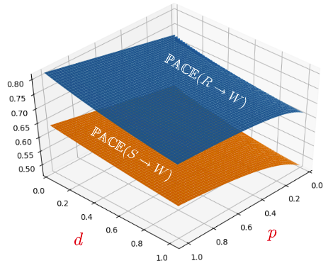
Figure 6. The blue and the orange surfaces are the PACEs of degree $d$ of $R$ and $S$ on $W$ as functions of $p$ and $d$, respectively.

Figure 7 shows the PACEs as a family of parametric curves that reveals PACEs changes more clearly.

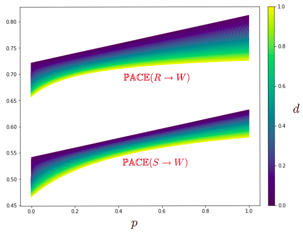
Figure 7. The top and the bottom plots represent the family of $d$-parameterized curves associated to the PACEs of degree $d$ of $R$ and $S$ on $W$ as functions of $p$, respectively. The color bar shows different values of $d\in[0,1]$.

5.3.2. Calculating the Counterfactual Using Our Framework

In the above example, assume that for any $(S,V_{3})=(s,v_{3})$, $W_{(s,v_{3})}(0)$ and $W_{(s,v_{3})}(1)$ denote the potential outcomes for $(R,S,V_{3})=(0,s,v_{3})$ and $(R,S,V_{3})=(1,s,v_{3})$, respectively. Now, assume that we observe $W_{(s,v_{3})}(0)=w$ for some $w\in\{0,1\}$ in such a way that $s$ and $v_{3}$ are unknowns. Now, we calculate $W_{(s,v_{3})}(1)$. To do so, we note that $w=0\oplus s\oplus v_{3}$, and hence $s\oplus v_{3}=w$. Thus, we have that

$$\mathbb{P}((s,v_{3})=(0,w)|W=w,R=0)=\frac{\mathbb{P}(s=0,v_{3}=w)}{\mathbb{P}(s=0,v_{3}=w)+\mathbb{P}(s=1,v_{3}=1-w)}.$$

First, assume that $w=0$, then we have that $(s,v_{3})\in\{(0,0),(1,1)\}$, and hence

$$\mathbb{P}((s,v_{3})=(0,0)|W=0,R=0) =\frac{0.6561}{0.6561+0.3(0.07+0.3p)}=\frac{0.6561}{0.6771+0.09p},$$

$$\mathbb{P}((s,v_{3})=(1,1)|W=0,R=0) =1-\mathbb{P}((s,v_{3})=(0,0)|W=w,R=0)$$

$$=\frac{0.021+0.09p}{0.6771+0.09p}.$$

Now, assume that $w=1$. Then, we have that $(s,v_{3})\in\{(0,1),(1,0)\}$, and hence

$$\mathbb{P}((s,v_{3})=(0,1)|W=1,R=0) =\frac{0.0439}{0.0439+0.3(0.93-0.3p)}=\frac{0.0439}{0.3229-0.09p},$$

$$\mathbb{P}((s,v_{3})=(1,0)|W=1,R=0) =1-\mathbb{P}((s,v_{3})=(0,1)|W=w,R=0)$$

$$=\frac{0.279-0.09p}{0.3229-0.09p}.$$

Finally, we calculate the probability distribution of $W_{(s,v_{3})}(1)$. To do so, we calculate $\mathbb{P}(W_{(s,v_{3})}(1)=0)$. When $R=1$ and $W=0$, we have that $s\oplus v_{3}=1$ and $s\neq 1$. It follows that $(s,v_{3})=(0,1)$. Thus,

$$\mathbb{P}(W_{(s,v_{3})}(1)=0) =\mathbb{P}((s,v_{3})=(0,1)|W=1,R=0)=\frac{0.0439}{0.3229-0.09p}.$$

Therefore, knowing $p$ gives us the probability distribution of $W_{(s,v_{3})}(1)$.

5.3.3. Calculating the ACDEs ̵‌of $R$ and $S$ on $W$.

We note that

$$\mathbb{P}(w) =\sum_{c,r,s,v_{1},v_{2},v_{3}}\mathbb{P}(c,r,s,v_{1},v_{2},v_{3},w)$$

$$=\sum_{c,r,s,v_{1},v_{2},v_{3}}\underbrace{\mathbb{P}(v_{2})\mathbb{P}(c|v_{2})\mathbb{P}(s|c,v_{2})}_{\mathbb{P}(c,s,v_{2})}\overbrace{\underbrace{\mathbb{P}(v_{1})}_{\mathbb{P}(v_{1}|c)}\mathbb{P}(r|c,v_{1})}^{\mathbb{P}(r,v_{1}|c)}\underbrace{\mathbb{P}(v_{3}|r,s)\mathbb{P}(w|r,s,v_{3})}_{\mathbb{P}(w,v_{3}|r,s)}$$

$$=\sum_{c,r,s}\mathbb{P}(c,s)\mathbb{P}(r|c)\mathbb{P}(w|r,s).$$

It follows that

$$\mathbb{P}(w|\mathrm{do}(r_{0})) =\sum_{c,s}\mathbb{P}(c,s)\mathbb{P}(w|r_{0},s)=\sum_{s}\mathbb{P}(s)\mathbb{P}(w|r_{0},s).$$

Thus,

$$\mathbb{P}(w|\mathrm{do}(r_{0},s_{0})) =\mathbb{P}(w|\mathrm{do}(r_{0},s_{0},(v_{3})_{0}))=\mathbb{P}(w|r_{0},s_{0}).$$

Similarly, we have that

$$\mathbb{P}(w|\mathrm{do}(s_{0})) =\sum_{r}\mathbb{P}(r)\mathbb{P}(w|r,s_{0}).$$

Thus, we have that

$$\mathbb{E}(W|\mathrm{do}(R=1)) =\mathbb{P}(W=1|\mathrm{do}(R=1))=\sum_{s=0}^{1}\mathbb{P}(s)\mathbb{P}(W=1|R=1,S=s)$$

$$=(0.7)(0.9)+(0.3)=0.93,$$

$$\mathbb{E}(W|\mathrm{do}(R=0)) =\mathbb{P}(W=1|\mathrm{do}(R=0))$$

$$=\sum_{s}^{1}\mathbb{P}(s)\mathbb{P}(W=1|R=0,S=s)$$

$$=(0.7)(0.01)+(0.3)(0.9)=0.277,$$

$$\mathbb{E}(W|\mathrm{do}(S=1)) =\mathbb{P}(W=1|\mathrm{do}(S=1))=\sum_{r=0}^{1}\mathbb{P}(r)\mathbb{P}(W=1|R=r,S=1)$$

$$=(0.5)(0.9)+(0.5)=0.95,$$

$$\mathbb{E}(W|\mathrm{do}(S=0)) =\mathbb{P}(W=1|\mathrm{do}(S=0))=\sum_{r=0}^{1}\mathbb{P}(r)\mathbb{P}(W=1|R=r,S=0)$$

$$=(0.5)(0.01)+(0.5)(0.9)=0.455.$$

Therefore, the ACE’s of $R$ and $S$ on $W$ are as follows:

$$\mathrm{ACE}(R\to W) =\mathbb{E}(W|\mathrm{do}(R=1))-\mathbb{E}(W|\mathrm{do}(R=0))$$

$$=0.93-0.277=0.653,$$

$$\mathrm{ACE}(S\to W) =\mathbb{E}(W|\mathrm{do}(S=1))-\mathbb{E}(W|\mathrm{do}(S=0))$$

$$=0.95-0.455=0.495.$$

Consequently, in this setting, similar to PACE, ACE calculates a higher causal effect for $R$ on $W$.

Now, we calculate the ACDEs of $R$ and $S$ on $W$ while controlling $S$ and $R$, respectively. To do so, by the above calculations, we have that

$$\mathrm{ACDE}\left((R\to W)|S\right) =\mathbb{E}_{S}\bigl{(}\mathbb{E}(W|\mathrm{do}(R=1,s))-\mathbb{E}(W|\mathrm{do}(R=0,s))\bigr{)}$$

$$=\mathbb{E}_{S}\bigl{(}\mathbb{P}(W=1|\mathrm{do}(R=1,s))-\mathbb{P}(W=1|\mathrm{do}(R=0,s))\bigr{)}$$

$$=\mathbb{E}_{S}\bigl{(}\mathbb{P}(W=1|R=1,s)-\mathbb{P}(W=1|R=0,s)\bigr{)}=0.653,$$

$$\mathrm{ACDE}\left((S\to W)|R\right) =\mathbb{E}_{R}\bigl{(}\mathbb{E}(W|\mathrm{do}(S=1,r))-\mathbb{E}(W|\mathrm{do}(S=0,r))\bigr{)}$$

$$=\mathbb{E}_{R}\bigl{(}\mathbb{P}(W=1|\mathrm{do}(S=1,r))-\mathbb{P}(W=1|\mathrm{do}(S=0,r))\bigr{)}$$

$$=\mathbb{E}_{R}\bigl{(}\mathbb{P}(W=1|S=1,r)-\mathbb{P}(W=1|S=0,r)\bigr{)}=0.495.$$

Therefore,

$$\mathrm{ACDE}\left((R\to W)|S\right)=\mathrm{ACE}(R\to W)>\mathrm{ACE}(S\to W)=\mathrm{ACDE}\left((S\to W)|R\right).$$

Finally, to calculate the ACDEs of $R$ and $S$ on $W$ while controlling $(S,V_{3})$ and $(R,V_{3})$, respectively, we note that:

$$\mathrm{ACDE}\left((R\to W)|S,V_{3}\right) =\mathrm{ACDE}\left((R\to W)|S\right)$$

$$>\mathrm{ACDE}\left((S\to W)|R\right)=\mathrm{ACDE}\left((S\to W)|R,V_{3}\right).$$

5.3.4. Calculating the Causal Strengths ̵‌of $R\to W$ and $S\to W$ Using Janzing et al. Framework

Let $\widetilde{\mathbb{P}}$ and $\widehat{\mathbb{P}}$ be the post-cutting distributions of the DAG in Figure 5 after cutting the arrows $R\to W$ and $S\to W$, respectively. Then, we have that

$$\mathbb{P}(c,r,s,w) =\mathbb{P}(c)\mathbb{P}(r|c)\mathbb{P}(s|c)\mathbb{P}(w|r,s),$$

$$\widetilde{\mathbb{P}}(c,r,s,w) =\mathbb{P}(c)\mathbb{P}(r|c)\mathbb{P}(s|c)\sum_{r^{\prime}}\mathbb{P}(w|r^{\prime},s)\mathbb{P}(r^{\prime}),$$

$$\widehat{\mathbb{P}}(c,r,s,w) =\mathbb{P}(c)\mathbb{P}(r|c)\mathbb{P}(s|c)\sum_{s^{\prime}}\mathbb{P}(w|r,s^{\prime})\mathbb{P}(s^{\prime}).$$

It follows that

$$D_{\mathrm{KL}}(\mathbb{P}||\widetilde{\mathbb{P}}) =\sum_{c,r,s,w}\mathbb{P}(c,r,s,w)\log\left(\frac{\mathbb{P}(c,r,s,w)}{\widetilde{\mathbb{P}}(c,r,s,w)}\right)$$

$$=\sum_{c,r,s,w}\mathbb{P}(c)\mathbb{P}(r|c)\mathbb{P}(s|c)\mathbb{P}(w|r,s)\log\left(\frac{\mathbb{P}(w|r,s)}{\sum_{r^{\prime}}\mathbb{P}(w|r^{\prime},s)\mathbb{P}(r^{\prime})}\right)\approx 0.351431,$$

$$D_{\mathrm{KL}}(\mathbb{P}||\widehat{\mathbb{P}}) =\sum_{c,r,s,w}\mathbb{P}(c,r,s,w)\log\left(\frac{\mathbb{P}(c,r,s,w)}{\widehat{\mathbb{P}}(c,r,s,w)}\right)$$

$$=\sum_{c,r,s,w}\mathbb{P}(c)\mathbb{P}(r|c)\mathbb{P}(s|c)\mathbb{P}(w|r,s)\log\left(\frac{\mathbb{P}(w|r,s)}{\sum_{s^{\prime}}\mathbb{P}(w|r,s^{\prime})\mathbb{P}(s^{\prime})}\right)\approx 0.270828.$$

Consequently, Janzing et al. framework as well as PACE and ACDE calculates a higher direct causal effect for $R$ on $W$.

5.3.5. Calculating the Causal Strengths ̵‌of $R\to W$ and $S\to W$ Using Mutual Information Fraework:

We have that

$$\mathbb{I}(R;W)=\mathbb{H}(W)-\mathbb{H}(W|R),\quad\mathbb{I}(S;W)=\mathbb{H}(W)-\mathbb{H}(W|S).$$

Hence, we need the probability distributions $\mathbb{P}(W),\mathbb{P}(W|R)$ and $\mathbb{P}(W|S)$. We have that

$$\mathbb{P}(W=1|R=1) =\sum_{s=0}^{1}\mathbb{P}(W=1|R=1,s)\mathbb{P}(s|R=1)$$

$$=(0.9)(0.82)+0.18=0.918,$$

$$\mathbb{P}(W=1|R=0) =\sum_{s=0}^{1}\mathbb{P}(W=1|R=0,s)\mathbb{P}(s|R=0)$$

$$=(0.01)(0.58)+(0.9)(0.42)=0.3838,$$

$$\mathbb{P}(W=1|S=1) =\sum_{r=0}^{1}\mathbb{P}(W=1|r,S=1)\mathbb{P}(r|S=1)$$

$$=(0.9)(0.7)+(0.3)=0.93,$$

$$\mathbb{P}(W=1|S=0) =\sum_{r=0}^{1}\mathbb{P}(W=1|r,S=0)\mathbb{P}(r|S=0)$$

$$=(0.01)\left(\frac{29}{70}\right)+(0.9)\left(\frac{41}{70}\right)=\frac{37.19}{70}.$$

It follows that

$$\begin{array}[]{lll}{\color[rgb]{0,0,1}\mathbb{P}(W|R=1)\sim\mathbb{B}(0.918)},&&{\color[rgb]{0,0,1}\mathbb{P}(W|R=0)\sim\mathbb{B}(0.3838)},\\ {\color[rgb]{0,0,1}\mathbb{P}(W|S=1)\sim\mathbb{B}(0.93)},&&{\color[rgb]{0,0,1}\mathbb{P}(W|S=0)\sim\mathbb{B}\left(\frac{37.19}{70}\right)}.\end{array}$$

Now, we calculate the probability distribution $\mathbb{P}(W)$ as follows:

$$\mathbb{P}(W=1)=\sum_{r=0}^{1}\mathbb{P}(W=1|r)\mathbb{P}(r)=0.5(0.3838+0.918)=0.6509.$$

Thus, we have that ${\color[rgb]{0,0,1}W\sim\mathbb{B}(0.6509)}$. One could see that

$$\mathbb{H}(W) \approx 0.933262,$$

$$\mathbb{H}(W|R) =\sum_{r=0}^{1}\mathbb{P}(r)\mathbb{H}(W|r)\approx 0.5(0.960682+0.409187)=0.6849345,$$

$$\mathbb{H}(W|S) =\sum_{s=0}^{1}\mathbb{P}(s)\mathbb{H}(W|s)\approx(0.7)(0.997174)+(0.3)(0.365924)=0.807799.$$

It follows that

$$\mathbb{I}(R;W) \approx 0.933262-0.6849345=0.2483275,$$

$$\mathbb{I}(S;W) \approx 0.933262-0.807799=0.125463.$$

5.3.6. Calculating the Causal Strengths ̵‌of $R\to W$ and $S\to W$ Using Conditional Mutual Framework

We have that

$$\mathbb{I}(R;W|S)=\mathbb{H}(W|S)-\mathbb{H}(W|R,S),\quad\mathbb{I}(S;W|R)=\mathbb{H}(W|R)-\mathbb{H}(W|R,S).$$

Hence, we need the joint distribution of $R$ and $S$. We have that $\mathbb{P}(r,s)=\mathbb{P}(r|s)\mathbb{P}(s)$, which implies that

$$\mathbb{P}(R=1,S=1) =(0.3)(0.3)=0.09,$$

$$\mathbb{P}(R=1,S=0) =\left(\frac{41}{70}\right)(0.7)=0.41,$$

$$\mathbb{P}(R=0,S=1) =(0.7)(0.3)=0.21,$$

$$\mathbb{P}(R=0,S=0) =\left(\frac{29}{70}\right)(0.7)=0.29.$$

Thus, we have that

$$\mathbb{H}(W|R,S) =\sum_{r,s=0}^{1}\mathbb{P}(r,s)\mathbb{H}(W|r,s)$$

$$\approx(0.29)(0.080793)+(0.21)(0.468996)+(0.41)(0.468996)=0.31420749.$$

Therefore, we have that

$$\mathbb{I}(R;W|S) \approx 0.807799-0.31420749=0.49359151,$$

$$\mathbb{I}(S;W|R) \approx 0.6849345-0.31420749=0.37072701.$$

6. Conclusion

In this paper, we defined a new causal framework to investigate causality via direct causal effects. Our framework includes a formula called PACE, which is an integration of two concepts: 1) intervention (via total variation), and 2) natural availability of changing the exposure/treatment values. The latter makes our framework distinct from the other well-known frameworks for causal reasoning. Further, our causal framework can handle both probabilistic and non-probabilistic causal problems using the parameter $d$ in PACE and its variations such as PEACE, SPACE, and APACE. Another notable property of our framework is to provide the facility for measuring direct causal effects of an exposure/treatment $X$ with respect to the changes that are allowed (e.g., in some real world problems, we may not be able to decrease the value of $X$. Consequently, PACE and PEACE are suitable formulas to measure the direct causal effect of $X$ on the outcome variable). Also, our ideas could be used in the Pearl/Neyman-Rubin frameworks to define new causal effect formulas, when $X$ is not necessarily binary.

A main controversial consequent of our framework is that the PACE of $X$ on $Y$ depends on the variables $\bm{\mathrm{Z}}$ that we are keeping constant. Hence, if we replace these variables $\bm{\mathrm{Z}}$ with their parents $\bm{\mathrm{W}}$ and update our causal relationships, then PACE would change. This is due to the fact that the ”natural availability of changing $X$ values given $\bm{\mathrm{Z}}$” is replaced with the ”natural availability of changing $X$ values given $\bm{\mathrm{W}}$” (however, one may think of this as a property and not a drawback!)

Currently, our framework only handles discrete random variables with finite possible values. For future works, we will add infinite discrete random variables and continuous random variables to our framework. Further, we will add fuzzy logic to our framework. Note that we previously built a fundamental probabilistic fuzzy logic (PFL) framework (see [40]). We showed that our PFL works well dealing with real world problems for which the criteria of selections are fuzzy. We will build an integration of our PFL and our causal inference framework to create a causal probabilistic variational fuzzy logic framework.

We will suggest other researchers study the mathematics of our variation formulas as probabilistic generalizations for the total variation of a function in mathematical analysis.

References

• [1] Holger Andreas and Mario Guenther, Regularity and inferential theories of causation, (2021).
• [2] Cesare Arzelà, Rend. Accad. Sci. Bologna 9:2 (1905), 100–107.
• [3] Kenneth A Bollen and Judea Pearl, Eight myths about causality and structural equation models, Handbook of causal analysis for social research, Springer, 2013, pp. 301–328.
• [4] Sarah Boslaugh, ”structural equation modeling”. encyclopedia of epidemiology, Sage Publications, 2007.
• [5] Lamberto Cesari, Sulle funzioni a variazione limitata, Annali della Scuola Normale Superiore di Pisa-Classe di Scienze 5 (1936), no. 3-4, 299–313.
• [6] Ennio De Giorgi and Luigi Ambrosio, Un nuovo tipo di funzionale del calcolo delle variazioni, Atti della Accademia Nazionale dei Lincei. Classe di Scienze Fisiche, Matematiche e Naturali. Rendiconti Lincei. Matematica e Applicazioni 82 (1988), no. 2, 199–210.
• [7] Otis Dudley Duncan, Introduction to structural equation models, Elsevier, 2014.
• [8] Nelson Dunford and Jacob T. Schwartz, Linear operators. I. General theory. (With the assistence of William G. Bade and Robert G. Bartle), Pure and Applied Mathematics. Vol. 7. New York and London: Interscience Publishers. xiv, 858 p. (1958)., 1958.
• [9] Fenwick W English, ”structural equation modeling”. encyclopedia of educational leadership and administration, Sage publications, 2006.
• [10] L Craig Evans and RF Gariepy, Studies in advanced mathematics, 1992.
• [11] Gaetano Fichera, Lezioni sulle trasformazioni lineari, vol. i, Istituto matematico dell’Università di Trieste (1954).
• [12] Pascal Getreuer, Rudin-osher-fatemi total variation denoising using split bregman, Image Processing On Line 2 (2012), 74–95.
• [13] Enrico Giusti, Minimal surfaces and functions of bounded variation, Monogr. Math., Basel, vol. 80, Birkhäuser, Cham, 1984 (English).
• [14] Madelyn Glymour, Judea Pearl, and Nicholas P Jewell, Causal inference in statistics: A primer, John Wiley & Sons, 2016.
• [15] Godfrey H Hardy, On double fourier series and especially those which represent the double zeta-function with real and incommensurable parameters, Quart. J. Math 37 (1906), no. 1, 53–79.
• [16] Jennifer Hill and Elizabeth Stuart, Causal inference: overview, International Encyclopedia of the Social & Behavioral Sciences: Second Edition (2015), 255–260.
• [17] Christopher Hitchcock, Probabilistic causation, (1997).
• [18] Guido W Imbens and Donald B Rubin, Causal inference in statistics, social, and biomedical sciences, Cambridge University Press, 2015.
• [19] Dominik Janzing, David Balduzzi, Moritz Grosse-Wentrup, and Bernhard Schölkopf, Quantifying causal influences, The Annals of Statistics 41 (2013), no. 5, 2324–2358.
• [20] Camille Jordan, Sur la série de fourier, Comptes rendus hebdomadaires des séances de l’Académie des sciences (in French) 92 (1881), 228–230.
• [21] Karl G Joreskog and Marielle Van Thillo, Lisrel: A general computer program for estimating a linear structural equation system involving multiple indicators of unmeasured variables., (1972).
• [22] Tessa Kennedy-Martin, Sarah Curtis, Douglas Faries, Susan Robinson, and Joseph Johnston, A literature review on the representativeness of randomized controlled trial samples and implications for the external validity of trial results, Trials 16 (2015), no. 1, 1–14.
• [23] Francesco Maggi, Sets of finite perimeter and geometric variational problems: an introduction to geometric measure theory, no. 135, Cambridge University Press, 2012.
• [24] David B Malament, The class of continuous timelike curves determines the topology of spacetime, Journal of mathematical physics 18 (1977), no. 7, 1399–1404.
• [25] William E May, Knowledge of causality in hume and aquinas, The Thomist: A Speculative Quarterly Review 34 (1970), no. 2, 254–288.
• [26] Peter Menzies and Helen Beebee, Counterfactual theories of causation, (2001).
• [27] Alyssa Ney, Physical causation and difference-making, The British Journal for the Philosophy of Science (2009).
• [28] Judea Pearl, Understanding propensity scores, Causality: models, reasoning, and inference 2 (2009), 348–352.
• [29] by same author, Direct and indirect effects, Probabilistic and Causal Inference: The Works of Judea Pearl, 2022, pp. 373–392.
• [30] by same author, Probabilities of causation: three counterfactual interpretations and their identification, Probabilistic and Causal Inference: The Works of Judea Pearl, 2022, pp. 317–372.
• [31] Judea Pearl et al., Models, reasoning and inference, Cambridge, UK: CambridgeUniversityPress 19 (2000), no. 2.
• [32] Judea Pearl and Dana Mackenzie, The book of why: the new science of cause and effect, Basic books, 2018.
• [33] J. Pierpont, Lectures on the theory of functions of real variables. Volume I., Boston, New York, Chicago, London: Ginn & Company. XII u. 560 S. gr. $8^{\circ}$ (1905)., 1905.
• [34] Richard Riegelman, Contributory cause: unnecessary and insufficient, Postgraduate medicine 66 (1979), no. 2, 177–179.
• [35] Alfred Arthur Robb, Optical geometry of motion: A new view of the theory of relativity, W. Heffer, 1911.
• [36] Paul R Rosenbaum and Donald B Rubin, The central role of the propensity score in observational studies for causal effects, Biometrika 70 (1983), no. 1, 41–55.
• [37] H. L. Royden, Real analysis, London: The Macmillan Company. xii, 349 p. (1969)., 1969.
• [38] Donald B Rubin, Estimating causal effects of treatments in randomized and nonrandomized studies., Journal of educational Psychology 66 (1974), no. 5, 688.
• [39] Leonid I Rudin, Stanley Osher, and Emad Fatemi, Nonlinear total variation based noise removal algorithms, Physica D: nonlinear phenomena 60 (1992), no. 1-4, 259–268.
• [40] Amir Saki and Usef Faghihi, A fundamental probabilistic fuzzy logic framework suitable for causal reasoning, arXiv preprint arXiv:2205.15016 (2022).
• [41] Stanislas Saks, Theory of the integral monografie matematyczne, Vol. VII., Warszawa-Lwow (1937).
• [42] MTCAJ Thomas and A Thomas Joy, Elements of information theory, Wiley-Interscience, 2006.
• [43] Leonida Tonelli, Sulle funzioni di due variabili generalmente a variazione limitata, Annali della Scuola Normale Superiore di Pisa-Classe di Scienze 5 (1936), no. 3-4, 315–320.
• [44] Robert R Tucci, Introduction to judea pearl’s do-calculus, arXiv preprint arXiv:1305.5506 (2013).
• [45] Guiseppe Vitali, Sui gruppi di punti e sulle funzioni di variabili reali, Atti Accad. Sci. Torino 43 (1908), 75–92.
• [46] A. I. Vol’pert, The spaces BV and quasilinear equations, Math. USSR, Sb. 2 (1968), 225–267 (English).
• [47] A. I. Vol’pert and S. I. Khudyaev, Analysis in classes of discontinuous functions and equations of mathematical physics, Mech.: Anal., vol. 8, Kluwer Academic Publishers Group, Dordrecht, 1985 (English).
• [48] Alfred North Whitehead, Process and reality, Simon and Schuster, 2010.
• [49] Phillip Wolff, Representing causation., Journal of experimental psychology: General 136 (2007), no. 1, 82.
• [50] Phillip Wolff and Aron K Barbey, Causal reasoning with forces, Frontiers in human neuroscience 9 (2015), 1.
• [51] James Woodward, Causation and manipulability, (2001).
• [52] Sewall Wright, The relative importance of heredity and environment in determining the piebald pattern of guinea-pigs, Proceedings of the National Academy of Sciences 6 (1920), no. 6, 320–332.
• [53] by same author, Correlation and causation, (1921).