Probabilistic Rank and Reward: A Scalable Model for Slate Recommendation

Abstract

We introduce Probabilistic Rank and Reward (PRR), a scalable probabilistic model for personalized slate recommendation. Our approach allows state-of-the-art estimation of the user interests in the ubiquitous scenario where the user interacts with at most one item from a slate of $K$ items. We show that the probability of a slate being successful can be learned efficiently by combining the reward, whether the user successfully interacted with the slate, and the rank, the item that was selected within the slate. PRR outperforms competing approaches that use one signal or the other and is far more scalable to large action spaces. Moreover, PRR allows fast delivery of recommendations powered by maximum inner product search (MIPS), making it suitable in low latency domains such as computational advertising.

1 INTRODUCTION

Recommender systems (advertising, search, music streaming, news, etc.) are becoming ubiquitous in society helping users navigate enormous catalogs of items to identify items relevant to their interests. In practice, recommender systems must optimize the content of an entire section of the user homepage which is viewed as a slate of $K$ items (Swaminathan et al., 2017). The slate often takes the form of a menu and the user can choose to interact with at most one of its items (Chen et al., 2019; Aouali et al., 2021). A slate of recommendations is considered successful if the user interacted with one of its items.

In practice, the number of items $P$ may be in the millions making the space of slates huge. This combinatorial nature of the space of slates makes learning very challenging. As an example, the performance of counterfactual estimators (Bottou et al., 2013; Swaminathan & Joachims, 2015), which are often based on inverse propensity scoring (IPS) (Horvitz & Thompson, 1952), deteriorates severely when the number of items is high as they can suffer extreme bias and variance. In particular, the bias issue is related to the fact that the logging policies often have deficient support (Sachdeva et al., 2020).

Another important challenge is the fast delivery of recommendations. A decision rule is an implementable mapping from what is known about the user to a slate of recommendations. Given a $d_{x}$-dimensional context vector $\bm{x}\in\mathcal{X}\subseteq{}^{d_{x}}$ that includes the user interests, the decision rule often boils down to solving ${\rm argmax}_{\bm{s}\in\mathcal{S}}L(\bm{x},\bm{s})$. Here $\mathcal{S}$ is the space of possible slates, and $L(\bm{x},\bm{s})$ is a score (or probability) associated with the slate $\bm{s}$ given the context $\bm{x}$. Unfortunately, this decision rule is not implementable since ${\rm argmax}_{\bm{s}\in\mathcal{S}}L(\bm{x},\bm{s})$ is intractable for large catalogs of items. Therefore, different proxy decision rules are used in practice, and they often aim at moving the search space from the combinatorially large set of slates $\mathcal{S}$ to a subset of the catalog of items $\{1,\ldots,P\}$. This is achieved by first associating a score for items instead of slates and then recommending the slate composed of the top-K items with the highest scores. This leads to a $\mathcal{O}(P)$ delivery time due to finding the top-K items. Unfortunately, this is not suitable for low-latency recommender systems with large catalogs. A common solution to improve this is the two-stage recommendation scheme. Here we first generate a small subset of potential item candidates $\mathcal{P}_{\rm sub}\subset\{1,\ldots,P\}$, and then select the top-K items in $\mathcal{P}_{\rm sub}$, which leads to a $\mathcal{O}(|\mathcal{P}_{\rm sub}|)$ delivery time.

The two-stage recommendation has three shortcomings. First, the scoring model, which selects the highest scoring items from $\mathcal{P}_{\rm sub}$, does not directly optimize the reward for the whole slate, and rather optimizes a proxy offline metric for each item individually. This induces numerous biases related to the layout of the slate such as position biases where users tend to interact more often with specific positions (Yue et al., 2010). Second, the candidate generation and the scoring models are not necessarily trained jointly, which may lead to having candidates in $\mathcal{P}_{\rm sub}$ that are not the highest scoring items. Third, the scoring model relies on small subsets of candidates, instead of optimizing for the whole catalog. Thus the reward signal might be much stronger since it is restricted to a small set of items, which may induce high bias.

Another practical approach to avoid the candidate generation step relies on approximate maximum inner product search (MIPS). MIPS algorithms are capable of quickly sorting $P$ items in roughly $\mathcal{O}(\log P)$ as long as the scores of items $a\in\{1,\ldots,P\}$ have the form $\bm{u}^{\top}\bm{\beta}_{a}$. Here $\bm{u}\in{}^{d}$ is a $d$-dimensional user embedding and $\bm{\beta}_{a}\in{}^{d}$ is the $d$-dimensional embedding of item $a$. This allows fast delivery of recommendation in roughly $\mathcal{O}(\log P)$ instead of $\mathcal{O}(P)$ without any additional candidate generation step.

An example of the output of PRR is shown in Fig. 1. In this situation, we imagine that a user is interested in technology. We show three candidate slates of size 2. In the left panel, the slate consists of two good recommendations: phone and microphone. The model predictions $(0.91,0.06,0.03)$ are the probabilities for no click, click on phone and click on microphone, respectively. Clearly, the probability of a click on slate phone, microphone is higher than the other slates, and is equal to 0.09. For comparison, the panel in the middle contains a good recommendation with the phone in the prime first position but the shoe in the second position, which is a poor match with the user interest in technology. As a consequence, the probabilities become $(0.94,0.04,0.01)$ for no click, click on phone and click on shoe. Finally, in the right panel, we show two poor recommendations of shoe and pillow resulting in the highest no-click probability $0.97$.

Figure 1: Example of 3 slates of size 2 on a technology website. From left to right are good, mixed and bad recommendations. $\bar{R},r_{1},r_{2}$ denote the actual probabilities of no-click, click on the first item and click on the second item, respectively.

Here the goal is to establish the level of association of each item (in this case phone, microphone, shoe and pillow) with a particular user interest (in this case technology). At first glance, analyzing logs of successful and unsuccessful recommendations is the best possible way to learn this association. However, in practice, there are numerous factors that influence the probability of a click other than the quality of recommendations. In this example, the non-click probability of the good recommendations (phone, microphone) is 0.91 (click probability of 0.09), while the non-click probability of the bad recommendations (shoe, pillow) is 0.97 (click probability of 0.03). The change in the click probability from good to bad recommendations is relatively modest at only 0.06. Thus the model must capture additional factors that influence clicks other than the quality of recommendations.

To account for this, PRR incorporates a real-world observation: the most informative features to predict successful interactions are engagement features. Such features summarize how likely the user is to interact with the slate independently of the quality of its recommendations. This includes for example the slate size and the level of user activity and engagement. While these features are strong predictors of interactions, they do not provide any information about which items are responsible for the interactions. In contrast, the recommendation features, which include the user interests and the items shown in the slate, provide a relatively modest signal for predicting interactions. However, they are very important for the recommendation task. Based on these observations, PRR uses the engagement features to accurately learn the parameters associated with the useful recommendation features. It may be useful to draw an analogy. Optical astronomers who take images of far-away galaxies need to develop a sophisticated understanding of many local phenomena: the atmosphere, the ambient light, the milky way, etc. The understanding of all these large effects allows them to construct precise images of extremely faint objects. Similarly, PRR is able to build a model of a weak recommendation signal by carefully capturing the other factors that often have high contributions to predicting the reward.

PRR also incorporates the information that different positions in the slate may have different properties. Some positions may boost a recommendation by making it more visible, and other positions may lessen the impact of the recommendation. To see this, consider the example in Fig. 1, the probability of clicking on shoes increased by $0.01$ when placed in the prime first position (slate in the middle) compared to placing it in the second position (slate in the right panel).

To summarize, our paper makes the following contributions. 1) We formalize the following ubiquitous slate recommendation setting. The user is shown a slate composed of $K$ items and they can choose to interact with at most one of the items in the slate. After that, the information received consists of two signals: did the user interact with one of the items? and if an item was interacted with, which item was it? We refer to these two types of signals as reward and rank, respectively. 2) We propose a likelihood-based probabilistic model (PRR) that combines both signals to learn efficiently. This is important as both, the reward and the rank, shall contain useful information about the user interests, and discarding one of them may lead to inferior performance. 3) PRRdistinguishes between slate-level and item-level features which contribute to an interaction with the slate and one of its items, respectively. PRR also incorporates the fact that interactions can be predicted by engagement features that neither represent the user interests nor the recommended items. Including such features help learn the recommendation signal more accurately. 4) The delivery of recommendations in PRR is reduced to solving a MIPS for $K$ items from a catalog of size $P$. While this constrains the parametric form of PRR, it makes it applicable to massive scale tasks with very low latency requirements such as computational advertising. 5) We show empirically that PRR outperforms commonly used baselines and that it is more scalable to large catalogs.

When compared to prior works, PRR enjoys the advantages of both worlds, reward and ranking based approaches. Reward based approaches (Dudík et al., 2012; Bottou et al., 2013) focus exclusively on the reward signal. This has a very profound advantage since what is optimized offline is aligned with the reward observed in A/B tests. However, the rank signal is ignored, and this loss of information makes learning difficult, especially for large catalogs and slates. On the other hand, learning in ranking approaches (Covington et al., 2016) is driven by heuristics focused on proxy information retrieval (IR) scores for individual items. This often leads to a striking gap between offline evaluation and A/B test results (see e.g., Section 5.1 in (Garcin et al., 2014)). PRR is similar to bandit approaches as it directly optimizes the reward as measured by A/B tests. It is also similar to ranking approaches as it makes use of the rank signal. However, PRR optimizes the reward for the whole slates instead of single items and incorporates other factors that may influence the reward independently of the quality of recommendations.

The remainder of this paper is organized as follows. In Section 2, we describe the setting for slate recommendation and our proposed algorithm. In Section 3, we review related work to the slate recommendation problem. In Section 4, we describe popular baselines and present our qualitative and quantitative results. In Section 5, we make concluding remarks and outline potential directions for future works.

2 PROPOSED ALGORITHM

2.1 Setting

For any positive integer $P$, we define $[P]=\{1,2,\ldots,P\}$. Vectors and matrices are denoted by bold letters. The $i$-th coordinate of a vector $\bm{x}$ is $x_{i}$; unless the vector is already indexed such as $\bm{x}_{j}$, in which case we write $x_{j,i}$. Let $\bm{A}\in{}^{P\times d}$ be a $P\times d$ matrix, the $d$-dimensional vector corresponding to the $i$-th row of $\bm{A}$ is denoted by $\bm{A}_{i}\in{}^{d}$ for any $i\in[P]$. Items are referenced by integers so that $[P]$ denotes the catalog of $P$ items. We define a slate of size $K$, $\bm{s}=\left(s_{1},\ldots,s_{K}\right)$, as a $K$-permutation of $[P]$, which is an ordered collection of $K$ items from $[P]$. The space of all slates of size $K$ is denoted by $\mathcal{S}$.

We consider the contextual bandit setting where the agent interacts with users as follows. The agent observes a $d_{x}$-dimensional context vector $\bm{x}\in\mathcal{X}\subseteq{}^{d_{x}}$. After that, the agent recommends a slate $\bm{s}\in\mathcal{S}$, and then receives a binary reward $R\in\{0,1\}$ and a list of $K$ binary ranks $[r_{1},\ldots,r_{K}]\in\{0,1\}^{K}$ that depend on both the context $\bm{x}$ and the slate $\bm{s}$. The reward $R$ indicates whether the user interacted with the slate $\bm{s}$ and for any $\ell\in[K]$ the rank $r_{\ell}$ indicates whether the user interacted with the $\ell$-th item in the slate, $s_{\ell}$. The user can interact with at most one item, and thus $R=\sum_{\ell\in[K]}r_{\ell}$. We let $\bar{R}=1-R$ so that $\bar{R}+\sum_{\ell\in[K]}r_{\ell}=1$.

We assume that the context $\bm{x}$ decomposes into two vectors as $\bm{x}=(\bm{y},\bm{z})$ where $\bm{y}\in{}^{d^{\prime}}$ and $\bm{z}\in{}^{d_{z}}$. Here $\bm{y}$ denotes the engagement features that are useful for predicting if an interaction with a slate will occur, independently of its items and the user interests. On the other hand, $\bm{z}\in\mathbb{R}^{d_{z}}$ denotes the remaining features in the context $\bm{x}$, which summarize the user interests. The dimension of $\bm{y}$ is fixed, while those of $\bm{z}$ and $\bm{x}$ are varying as they can contain the list of previously viewed items. Table 1 summarizes our notation. It also includes new quantities that we use and explain in the sequel.

Notation	Definition
$\bm{x}=(\bm{y},\bm{z})\in\mathbb{R}^{d_{x}}$	context.
$\bm{y}\in\mathbb{R}^{d^{\prime}}$	engagement features.
$\bm{z}\in\mathbb{R}^{d_{z}}$	user interestsfeatures.
$R\in\{0,1\}$	reward indicator.
$\bar{R}\in\{0,1\}$	regret indicator.
$r_{\ell}\in\{0,1\}$	rank indicator of the item in position $\ell\in[K]$.
$\bm{\phi}\in\mathbb{R}^{d^{\prime}}$	bidding parameters.
$\gamma_{\ell}\in\real$	multiplicative position bias in position $\ell\in[K]$.
$\alpha_{\ell}\in\real$	additive position bias in position $\ell\in[K]$.
$g_{\bm{\Gamma}}(\bm{z})\in{}^{d}$	user embedding.
$\bm{\Psi}\in{}^{P\times d}$	items embeddings.
$\theta_{0}\in\real$	score for no-interaction with the slate.
$\theta_{\ell}\in\real$	score for an interaction with the item in position $\ell\in[K]$.
$\bm{s}=(s_{1},...,s_{K})$	slate of $K$ recommendations $s_{\ell}\in[P]$ for any $\ell\in[K]$.

Table 1: Notation.

2.2 Modeling Rank and Reward

As highlighted previously, our approach accounts for an important observation made by practitioners. It is often possible to produce a good model for predicting interactions with slates while discarding user interests and the items recommended to the user. Instead, engagement features such as the slate size, its attractiveness and the level of user activity can be strong predictors of interactions. While a model using only these features might have an excellent ability to predict interactions and thus high likelihood, it is useless for recommendation. This observation is often used to justify abandoning likelihood-based approaches for recommendation in favor of greedy ranking. Instead, PRR solves this issue by carefully incorporating both the engagement features $\bm{y}$, the user interests features $\bm{z}$ and the whole slate $\bm{s}$ to predict interactions accurately. Precisely, the PRR model has the following form

$$\bar{R},r_{1},\ldots,r_{K}|\bm{x},\bm{s}\sim{\rm cat}\left(\frac{\theta_{0}}{Z},\frac{\theta_{1}}{Z},\ldots,\frac{\theta_{K}}{Z}\right),\quad Z=\sum_{k=0}^{K}\theta_{\ell},$$ (1)

where $\bar{R},r_{1},\ldots,r_{K}$ and $\bm{x}=(\bm{y},\bm{z})$ are defined in Section 2.1, $\rm cat()$ is the categorical distribution, $\theta_{0}$ is the score of no interaction with the slate and $\theta_{\ell}$, for $\ell\in[K]$ is the score of interaction with the $\ell$-th item in the slate, $s_{\ell}$. We discuss how to derive these scores next.

The engagement features $\bm{y}$ are used to produce a positive score $\theta_{0}$ which is high if the chance of no interaction with the slate is high, independently of its items. That is

$$\theta_{0}=\exp(\bm{y}^{\top}\bm{\phi}),$$ (2)

where $\bm{\phi}$ is a vector of learnable parameters of dimension $d^{\prime}>0$. Similarly, the positive score $\theta_{\ell}$ is associated with the item in position $\ell$ in the slate, $s_{\ell}$, and is calculated in a way that captures user interests, position biases, and interactions that occur by accident. Precisely, given a slate $\bm{s}=(s_{1},\ldots,s_{K})$ and user interests features $\bm{z}$, the score $\theta_{\ell}$ has the following form

$$\theta_{\ell}=\exp\{g_{\bm{\Gamma}}(\bm{z})^{\top}\bm{\Psi}_{s_{\ell}}\}\exp(\gamma_{\ell})+\exp(\alpha_{\ell}).$$ (3)

Again this formulation is motivated by practitioners experience. The quantity $\exp(\alpha_{\ell})$ denotes the additive bias for position $\ell\in[K]$ in the slate. It is high if there is a high chance of interaction with the $\ell$-th item in the slate irrespective of how appealing it is to the user. This quantity also explains clicks that are not associated at all with the recommendation (e.g., clicks by accident). For instance, the probability of a click on slates is always larger than $\sum_{\ell\in[K]}\exp(\alpha_{\ell})/Z$. The quantity $\exp(\gamma_{\ell})$ is the multiplicative bias for position $\ell\in[K]$. It is high if a recommendation is boosted by being in position $\ell\in[K]$. To see the importance of biases $\exp(\gamma_{\ell})$, consider a slate of size 10 where the first and last items are {phone,…, microphone} and suppose that the user clicked on phone. Then from a ranking perspective, we would assume that the user prefers the phone over the microphone. But the user might have clicked on the phone just because it was placed in the top position. PRR captures this through the multiplicative terms $\exp(\gamma_{\ell})$.

The main quantity of interest is the recommendation score $g_{\bm{\Gamma}}(\bm{z})^{\top}\bm{\Psi}_{a}$ for $a\in[P]$, which can be understood as follows. The vector $\bm{z}\in{}^{d_{z}}$ represents the user interests and the parameter vector $\bm{\Psi}_{s_{\ell}}\in\mathbb{R}^{d}$ represents the embedding of the $\ell$-th item in the slate, $s_{\ell}$. The vector $\bm{z}$ is first mapped into a fixed size $d$-dimensional embedding space using $g_{\bm{\Gamma}}(\cdot)$. The resulting inner product $g_{\bm{\Gamma}}(\bm{z})^{\top}\bm{\Psi}_{s_{\ell}}$ produces a positive or negative score that quantifies how good $s_{\ell}$ is to the user with interests $\bm{z}$. In practice, $\bm{z}$ can be the sequence of previously viewed items, in which case $g_{\bm{\Gamma}}$ is a sequence model (Hochreiter & Schmidhuber, 1997; Vaswani et al., 2017).

2.3 Learning

PRR has multiple parameters $\bm{\phi},\bm{\bm{\Gamma}},\bm{\Psi},\gamma_{\ell},$ and $\alpha_{\ell}$ for $\ell\in[K]$, which are learned using the maximum likelihood principle. Precisely, we assume access to logged data $\mathcal{D}_{n}$ of the form

$$\mathcal{D}_{n}=\{\bm{x}_{i},\bm{s}_{i},\bar{R}_{i},r_{i,1},\ldots,r_{i,K}\,;i\in[n]\}\,,$$

such that $\bm{x}_{i}=(\bm{y}_{i},\bm{z}_{i})$ for any $i\in[n]$. Let $Z_{i}=\exp(\bm{y}_{i}^{\top}\bm{\phi})+\sum_{\ell\in[K]}\exp\{g_{\bm{\Gamma}}(\bm{z}_{i})^{\top}\bm{\Psi}_{s_{i,\ell}}\}\exp(\gamma_{\ell})+\exp(\alpha_{\ell})$ be the normalizing constant for the $i$-th data-point in $\mathcal{D}_{n}$, then log-likelihood reads

$$\mathcal{L}(\mathcal{D}_{n};\bm{\phi},\bm{\Gamma},\bm{\Psi},\bm{\gamma},\bm{\alpha}) =\sum_{i\in[n]}\log P(\bar{R}_{i},r_{i,1},\ldots,r_{i,K}\mid\bm{x}_{i},\bm{s}_{i},\bm{\phi},\bm{\Gamma},\bm{\Psi},\bm{\gamma},\bm{\alpha})\,,$$ (4)

$$=\sum_{i\in[n]}\left(\bm{y}_{i}^{\top}\bm{\phi}\right)\mathbb{I}_{\{\bar{R}_{i}=1\}}+\left(\log\left(\exp\{g_{\bm{\Gamma}}(\bm{z}_{i})^{\top}\bm{\Psi}_{s_{i,\ell}}\}\exp(\gamma_{\ell})+\exp(\alpha_{\ell})\right)\right)\mathbb{I}_{\{r_{i,\ell}=1\}}-\log(Z_{i})\,.$$

Finally, we maximize the log-likelihood to estimate the parameters as

$$\hat{\bm{\phi}}_{n},\hat{\bm{\Gamma}}_{n},\hat{\bm{\Psi}}_{n},\hat{\bm{\gamma}}_{n},\hat{\bm{\alpha}}_{n}={\rm argmax}_{\bm{\phi},\bm{\Gamma},\bm{\Psi},\bm{\gamma},\bm{\alpha}}\mathcal{L}(\mathcal{D}_{n};\bm{\phi},\bm{\Gamma},\bm{\Psi},\bm{\gamma},\bm{\alpha})\,.$$

In the sequel, with slight abuse of notation, we refer to the learned parameters $\hat{\bm{\phi}}_{n},\hat{\bm{\Gamma}}_{n},\hat{\bm{\Psi}}_{n},\hat{\bm{\gamma}}_{n},\hat{\bm{\alpha}}_{n}$ by $\bm{\phi},\bm{\Gamma},\bm{\Psi},\bm{\gamma},\bm{\alpha}$ for ease of exposition.

2.4 Decision Making

Given Eqs. 2 and 3, we know that the probability of an interaction with the slate is

$$P(R=1\mid\bm{x},\bm{s})=1-P(\bar{R}=1\mid\bm{x},\bm{s})=1-\frac{\theta_{0}}{Z}=1-\frac{\theta_{0}}{\theta_{0}+\sum_{\ell\in[K]}\theta_{\ell}}\,.$$ (5)

The decision rule follows as

$${\rm argmax}_{\bm{s}\in\mathcal{S}}P(R=1\mid\bm{x},\bm{s}) ={\rm argmin}_{\bm{s}\in\mathcal{S}}\frac{\theta_{0}}{\theta_{0}+\sum_{\ell\in[K]}\theta_{\ell}}\,,$$

$$\stackrel{{\scriptstyle(i)}}{{=}}{\rm argmax}_{\bm{s}\in\mathcal{S}}\sum_{\ell\in[K]}\theta_{\ell}\,,$$

$$={\rm argmax}_{\bm{s}\in\mathcal{S}}\sum_{\ell\in[K]}\exp\{g_{\bm{\Gamma}}(\bm{z})^{\top}\bm{\Psi}_{s_{\ell}}\}\exp(\gamma_{\ell})+\exp(\alpha_{\ell})\,$$

$$\stackrel{{\scriptstyle(ii)}}{{=}}{\rm argmax}_{\bm{s}\in\mathcal{S}}\sum_{\ell\in[K]}\exp\{g_{\bm{\Gamma}}(\bm{z})^{\top}\bm{\Psi}_{s_{\ell}}\}\exp(\gamma_{\ell})\,,$$ (6)

where $(i)$ and $(ii)$ follow from the fact that both $\theta_{0}$ and $\exp(\alpha_{\ell})$ are additive and do not depend on $\bm{s}$. Our goal is to reduce decision-making to a MIPS task. Thus the parametric form $\bm{u}^{\top}\bm{\beta}$ must be satisfied, which means that the sum $\sum_{\ell\in[K]}$, the exponential in $\exp\{g_{\bm{\Gamma}}(\bm{z})^{\top}\bm{\Psi}_{s_{\ell}}\}$ and the term $\exp(\gamma_{\ell})$ in Eq. 6 need to be removed. This is achieved by first performing a MIPS as

$$s_{1}^{\prime},\ldots,s_{K}^{\prime}={\rm argsort}(g_{\bm{\Gamma}}(\bm{z})^{\top}\bm{\Psi})_{1:K}\,.$$ (7)

We then sort the position biases as

$$i_{1},\ldots,i_{K}={\rm argsort}(\gamma)\,.$$ (8)

Finally, the recommended slate $\bm{s}=(s_{1},s_{2},\ldots,s_{K})$ is obtained by rearranging the items $s_{1}^{\prime},\ldots,s_{K}^{\prime}$ as

$$s_{1},s_{2},\ldots,s_{K}=s_{i_{1}}^{\prime},s_{i_{2}}^{\prime},\ldots,s_{i_{K}}^{\prime}\,.$$ (9)

In other terms, we select the Top-K items with the highest recommendation scores $g_{\bm{\Gamma}}(\bm{z})^{\top}\bm{\Psi}_{a}$ for $a\in[P]$. We then place the highest scoring item into the best position, that is the position $\ell\in[K]$ with the largest value of $\exp(\gamma_{\ell})$. Then the second-highest scoring item is placed into the second-best position, and so on. The procedure in Eqs. 7, 8 and 9 is equivalent to the decision rule in Eq. 6. It is also computationally efficient as Eq. 7 can be performed roughly in $\mathcal{O}(\log P)$ thanks to fast approximate MIPS algorithms (Abbasifard et al., 2014; Ding et al., 2019), while Eq. 6 requires roughly $\mathcal{O}(P^{K})$. The time complexity is also improved compared to ranking approaches by $\mathcal{O}(P/\log P)$. This makes PRR scalable to huge catalogs.

Note that $\bm{\phi},\bm{\alpha}$ are nuisance parameters as they are not needed for decision making; only the recommendation scores $g_{\bm{\Gamma}}(\bm{z})^{\top}\Psi_{a}$ and the multiplicative position biases $\exp(\gamma_{\ell})$ are used in the procedure in Eqs. 7, 8 and 9. While not used in decision-making, learning these parameters is necessary to accurately predict the recommendation scores. Also, including them in the model provides room for interpretability in some cases.

To summarize, PRR has the following properties. 1) It models the joint distribution of the reward and ranks $(\bar{R},r_{1},\ldots,r_{K})$ in the simple formulation given in Eq. 1. 2) It makes use of engagement features $\bm{y}$ in order to help learn the recommendation signal more accurately. 3) Its recommendation scores have a parametric form that is suitable for MIPS, which allows fast delivery of recommendations in $\mathcal{O}(\log P)$.

3 RELATED WORK

Reward optimizing recommendation aims at directly optimizing the reward using logged data. The earliest work (Dudík et al., 2012) used inverse propensity scoring (IPS) (Horvitz & Thompson, 1952) to estimate the reward for recommendation tasks with small action spaces. Unfortunately, IPS can suffer high bias and variance in realistic settings. This is mainly driven by two practical factors; the action space is combinatorially large and the logging policies primarily exploit certain recommendations with minimal exploration making their support deficient (Sachdeva et al., 2020).

The high variance of IPS is acknowledged and several fixes have been proposed. This includes clipping and self-normalizing importance weights (Gilotte et al., 2018). Unfortunately, in practice, altering the IPS estimator in these ways has the impact of avoiding recommendations about which little is known. This causes the learned policy to be close to the logging policy. Another solution is doubly robust (DR) (Dudík et al., 2014) which uses a reward model as control variate for IPS to reduce the variance. DR relies on a reward model and PRR can be integrated into it.

In slate recommendation, recent works made simplifying structural assumptions to reduce the variance. For instance, Li et al. (2018) restricted the search space by assuming that items contribute to the reward individually. Similarly, Swaminathan et al. (2017) assumed that slate-level reward is additive w.r.t. unobserved and independent ranks. The independence assumption is restrictive and can be violated in many production settings. Also, the learned policy might recommend slates with repeated items, which is illegal. A relaxed assumption was proposed in (McInerney et al., 2020) where the interaction between the user and the $\ell$-th item in the slate, $s_{\ell}$, depends only on $s_{\ell}$, $s_{\ell-1}$ and its rank $r_{\ell-1}$. This sequential dependence scheme is not sufficient to encode the ubiquitous setting where the user views the whole slate at once and interacts with at most one of its items.

Another popular family of methods is click models (Chuklin et al., 2015). The simplest is click-through-rate models which defines a single parameter for the probability that an item is clicked, possibly depending on its position or the user (Joachims et al., 2017; Craswell et al., 2008). Another type is called cascade models (Dupret & Piwowarski, 2008; Guo et al., 2009; Chapelle & Zhang, 2009), which is suitable when items are presented in sequential order. Later, these models were extended to accommodate multiple user sessions (Chuklin et al., 2013; Zhang et al., 2011), granularity levels (Hu et al., 2011; Ashkan & Clarke, 2012), and additional user signals (Huang et al., 2012; Liu et al., 2014). Click models are often represented as graphical models and as such define dependencies manually and are not always scalable to large action spaces. Also, they were primarily designed for search engine retrieval and often do not incorporate extra features that are available in recommendation tasks.

Some works on slate recommendation focused on the idea that there are interactions between items within the slates making certain combinations of recommended items virtuous (or not) (Ie et al., 2019; Jiang et al., 2019; Wilhelm et al., 2018; Zhao et al., 2018). While it is possible to incorporate such interactions in our model formulation, it is unclear if it will be possible to reduce decision-making to a MIPS task.

4 EXPERIMENTS

We opt for simulation to evaluate PRR as it mimics the actual sequential interaction between users and recommender systems. The other alternatives consist in either using offline proxy information-retrieval metrics or using off-policy evaluation through IPS. Unfortunately, the former is often not aligned with online A/B test results, while the latter can suffer high bias and variance in large-scale settings (Aouali et al., 2022).

4.1 Experimental Design

We design a simulated A/B test protocol that takes different recommender systems as input and outputs their respective reward. We first define the problem instance consisting of the true parameters (oracle) and the logging policy as $\{\bm{\phi},\bm{\gamma},\bm{\alpha},g_{\bm{\Gamma}}(\cdot),\bm{\Psi},P_{\bm{y}}(\cdot),P_{\bm{z}}(\cdot),P_{K}(\cdot)\}$ and $\pi_{0}$. Here $P_{\bm{y}}(\cdot),P_{\bm{z}}(\cdot)$, and $P_{K}(\cdot)$ are the distributions of the engagement features, the user interests features and the slate size, respectively. Given the oracle, we produce offline training logs and propensity scores $\{\mathcal{D},\mathcal{P}\}$ by running the logging policy $\pi_{0}$ as described in Algorithm 1. These logs are then used to train PRR and competing baselines. After training, the simulated A/B test in Algorithm 2 is used for testing.

We consider two non-personalized logging policies. (a) uniform:this policy samples uniformly without replacement $K$ items from the catalog $[P]$. That is $\pi_{0}(\bm{s}\mid\bm{z})=\frac{1}{P(P-1)\ldots(P-K+1)}$ for any slate $\bm{s}\in\mathcal{S}$ and any user interests $\bm{z}$. (b) top-K pop:this policy samples without replacement $K$ items where the probability of an item $a$ is proportional to the $L_{2}$ norm of its embedding, $\|\bm{\Psi}_{a}\|$. This is based on the intuition that a large value of $\|\bm{\Psi}_{a}\|$ means that item $a$ is recommended more often and thus it is more popular. We stress that this logging policy has access to the true embeddings $\bm{\Psi}$ of the simulated environment (Algorithm 1). Now we present the baselines to which we compare PRR.

Input: oracle parameters $\{\bm{\phi},\gamma,\alpha,g_{\bm{\Gamma}}(\cdot),\bm{\Psi},P_{\bm{y}}(\cdot),P_{\bm{z}}(\cdot),P_{K}(\cdot)\}$, logging policy $\pi_{0}(\bm{s}\mid\bm{x})$, marginal logging policies $\pi_{0}(s_{1}|\bm{x}),\ldots,\pi_{0}(s_{K}|\bm{x})$, $n_{\rm train}$.

Output: logs $\mathcal{D}$, propensity scores $\mathcal{P}$.

$\mathcal{D}\leftarrow\{\,\}\,,\quad\mathcal{P}\leftarrow\{\,\}$

for $i=1,\ldots,n_{\rm train}$ do

       $\bm{y}_{i}\sim P_{\bm{y}}(\cdot)\,,\quad\bm{z}_{i}\sim P_{\bm{z}}(\cdot)\,,\quad K_{i}\sim P_{K}(\cdot)$ ,  $\bm{x}_{i}=[\bm{y}_{i},\bm{z}_{i}]$ ,  $\bm{s}_{i}=[s_{i,1},\ldots,s_{i,K_{i}}]\sim\pi_{0}(\cdot|\bm{x}_{i})$

       $\theta_{0}\leftarrow\exp(\bm{y}_{i}^{\top}\bm{\phi})$

       for $k=1,\ldots,K$ do

            $\theta_{k}\leftarrow\exp(g_{\bm{\Gamma}}(\bm{z}_{i})^{\top}\bm{\Psi}_{a_{k}})\exp(\gamma_{k})+\exp(\alpha_{k})$

       end for

      $\bar{R}_{i},r_{i,1},\ldots,r_{i,K}\sim{\rm cat}\left(\frac{\theta_{0}}{Z},\frac{\theta_{1}}{Z},\ldots,\frac{\theta_{K}}{Z}\right)\,,\quad Z=\sum_{\ell=0}^{K_{i}}\theta_{\ell}$

       $\mathcal{D}\leftarrow\mathcal{D}\cup\{\bm{x}_{i},\bm{s}_{i},\bar{R}_{i},r_{i,1},\ldots,r_{i,K}\}$

       $\mathcal{P}\leftarrow\mathcal{P}\cup\{\pi_{0}(\bm{s}_{i}|\bm{x}_{i}),\pi_{0}(s_{i,1}|\bm{x}_{i}),\ldots,\pi_{0}(s_{i,K}|\bm{x}_{i})\}$

end for

Algorithm 1 Simulated Training Logs

Input: oracle parameters $\{\bm{\phi},\gamma,\alpha,g_{\bm{\Gamma}}(\cdot),\bm{\Psi},P_{\bm{y}}(\cdot),P_{\bm{z}}(\cdot),P_{K}(\cdot)\}$, decision rule $d_{\textsc{a}}$, decision rule $d_{\textsc{b}}$, $n_{\rm test}$.

Output: lists of rewards $R_{\textsc{a}}$ and $R_{\textsc{b}}$.

$R_{\textsc{a}}\leftarrow\{\;\}\,,\quad R_{\textsc{b}}\leftarrow\{\;\}$

for $i=1,\ldots,n_{\rm test}$ do

       for $\textsc{m}\in\{\textsc{a},\textsc{b}\}$ do

             $\bm{y}_{i}\sim P_{\bm{y}}(\cdot)\,,\quad\bm{z}_{i}\sim P_{\bm{z}}(\cdot)\,,\quad K_{i}\sim P_{K}(\cdot)$

             $\bm{s}_{i}=[s_{i,1},\ldots,s_{i,K_{i}}]\leftarrow d_{\textsc{m}}(\bm{y}_{i},\bm{z}_{i})$

             $\theta_{0}\leftarrow\exp(\bm{y}_{i}^{\top}\bm{\phi})$

             for $k=1,\ldots,K_{i}$ do

                  $\theta_{k}\leftarrow\exp(g_{\bm{\Gamma}}(\bm{z}_{i})^{\top}\bm{\Psi}_{s_{i,k}})\exp(\gamma_{k})+\exp(\alpha_{k})$

             end for

            $R_{\textsc{a}}\leftarrow R_{\textsc{a}}\cup\{1-\frac{\theta_{0}}{Z}\}\,,\quad Z=\sum_{\ell=1}^{K_{i}}\theta_{\ell}$

       end for

      

end for

Algorithm 2 Simulated A/B Test

Variants of PRR: we consider three variants of PRR. First, PRR-reward uses only the reward and ignores the rank signal. PRR-reward is trained on both, successful and unsuccessful slates. Second, PRR-rank discards the reward and is consequently trained on successful slates only. Finally, PRR-bias ignores the engagement features $\bm{y}$, in which case $\theta_{0}=\phi$ where $\phi$ is a scalar parameters ($\phi$ replaces $\exp(\bm{y}^{\top}\bm{\phi})$ in PRR). The goal of comparing PRR to PRR-reward and PRR-rank is to showcase the benefit of combining both signals, while comparing it to PRR-bias is to highlight the effect and importance of the engagement features.

PRR-reward: $$\bar{R},r_{1},\ldots,r_{K}\mid\bm{x},\bm{s}\sim{\rm cat}\Big{(}\frac{\theta_{0}}{Z},\frac{\sum_{\ell=1}^{K}\theta_{\ell}}{Z}\Big{)},\quad Z=\sum_{\ell=0}^{K}\theta_{\ell}\,,$$

PRR-rank: $$r_{1},\ldots,r_{K}\mid\bm{x},\bm{s}\sim{\rm cat}\Big{(}\frac{\theta_{1}}{Z},\ldots,\frac{\theta_{K}}{Z}\Big{)},\quad Z=\sum_{\ell=1}^{K}\theta_{\ell}\,,$$

PRR-bias: $$\bar{R},r_{1},\ldots,r_{K}\mid\bm{x},\bm{s}\sim{\rm cat}\Big{(}\frac{\phi}{Z},\frac{\theta_{1}}{Z},\ldots,\frac{\theta_{K}}{Z}\Big{)},\quad Z=\phi+\sum_{\ell=1}^{K}\theta_{\ell}.$$

where $\theta_{0}$ and $\theta_{\ell}$ for $\ell\in[K]$ are defined in Eqs. 2 and 3 while $\phi\in\real$ in PRR-bias is a learnable parameter.

Inverse propensity scoring: here unbiased estimators of the expected reward of policies are designed by removing the preference bias of the logging policy $\pi_{0}$ in data $\mathcal{D}$. This is achieved by re-weighting samples using the discrepancy between the new policy $\pi$ and the logging policy $\pi_{0}$ such as

$$\hat{V}_{n}^{\rm IPS}(\pi) =\frac{1}{n}\sum_{i=1}^{n}R_{i}\frac{\pi(\bm{s}_{i}|\bm{z}_{i})}{\pi_{0}(\bm{s}_{i}|\bm{z}_{i})}\,.$$ (10)

The IPS estimator above is provably unbiased when $\pi$ and $\pi_{0}$ have common support, but can suffer large variance. It can also be highly unbiased when the common support assumption is violated (Sachdeva et al., 2020), which is common in practice. One way to mitigate this is to reduce the action space from slates to items (Li et al., 2018). This is achieved by assuming that the reward $R$ is the sum of rank $r_{1},\ldots,r_{K}$, and that the $\ell$-th rank, $r_{\ell}$, only depends on the item $s_{\ell}$ and its position $\ell$. This allows estimating the expected reward of policy $\pi$ as

$$\hat{V}^{\rm IIPS}(\pi) =\frac{1}{n}\sum_{i=1}^{n}\sum_{\ell=1}^{K}r_{i,\ell}\frac{\pi(s_{i,\ell},\ell|\bm{z}_{i})}{\pi_{0}(s_{i,\ell},\ell|\bm{z}_{i})}\,,$$ (11)

where $\pi(a,\ell|\bm{z})$ and $\pi_{0}(a,\ell|\bm{z})$ are the marginal probabilities that the policy $\pi$ and the logging policy $\pi_{0}$ place the item $a$ in position $\ell\in[K]$ given user interests $\bm{z}$, respectively.

The next step is to optimize the estimator ($\hat{V}_{n}^{\rm IPS}(\pi)$ or $\hat{V}_{n}^{\rm IIPS}(\pi)$) to find the policy that will be used for decision-making (Swaminathan & Joachims, 2015). To achieve this, we need to parameterize the learning policy $\pi$. A common solution is to use factorized policies. While convenient, factorization causes the learned policy to converge to selecting slates with repeated items, which is illegal. Thus we opt for Plackett-Luce policies which are defined as follows. First, the probability of an item $a\in[P]$ is parametrized as

$$p_{\Xi,\beta}(a|\bm{z})=\frac{\lambda_{a}}{\sum_{a^{\prime}\in[P]}\lambda_{a^{\prime}}}\,, \lambda_{a}=\exp\{f_{\bm{\Xi}}(\bm{z})^{\top}\bm{\beta}_{a}\}\quad\forall a\in[P]\,,$$

where $\bm{\beta}_{a}\in{}^{d}$ is the embedding of item $a$ and $f_{\bm{\Xi}}$ maps user interests $\bm{z}\in{}^{d_{z}}$ into a $d$-dimensional embedding. Then the learning policy $\pi$ is parametrized as $\pi_{\Xi,\beta,K}$ and written as

$$\pi_{\Xi,\beta,K}(\bm{s}|\bm{z})=\frac{\lambda_{s_{1}}}{Z}\ \frac{\lambda_{s_{2}}}{Z-\lambda_{s_{1}}}\ \cdots\ \frac{\lambda_{s_{K}}}{Z-\sum_{j=1}^{K-1}\lambda_{s_{j}}}=\prod_{\ell=1}^{K}\frac{\lambda_{s_{\ell}}}{Z-\sum_{j=1}^{\ell-1}\lambda_{s_{j}}}\,, Z=\sum_{a^{\prime}\in[P]}\lambda_{a^{\prime}}\,.$$ (12)

Sampling from $\pi_{\Xi,\beta,K}(\cdot|\bm{z})$ is equivalent to sampling without replacement $K$ items from $[P]$ where the probability of item $a\in[P]$ is $p_{\Xi,\beta}(a|\bm{z})$. Finally, $\hat{V}_{n}^{\rm IIPS}(\pi)$ also requires computing the marginal probabilities $\pi(a,\ell|\bm{z})$ and $\pi_{0}(a,\ell|\bm{z})$, which can be intractable. Here we simply approximate $\pi_{0}(a,\ell|\bm{z})\approx\|\Psi_{a}\|/{\sum_{a^{\prime}}\|\Psi_{a^{\prime}}\|}$ for the top-K pop logging policy and $\pi(a,\ell|\bm{z})\approx p_{\Xi,\beta}(a|\bm{z})$ for the learning policies. Approximation is not needed for the uniform logging policy as we have that $\pi_{0}(a,\ell|\bm{z})=1/P$.

Top-K heuristic: we also use the top-K heuristic developed in (Chen et al., 2019) which causes the probability mass in $\pi_{\Xi,\beta,K}(\bm{s}|\bm{z})$ to be spread out over the top-K high scoring items. The top-K heuristic has a parameter $K^{*}$ that controls the number of items that the policy should spread over. We set it to 3 in our experiments, which we found to be good for the relatively small slate sizes we were considering.

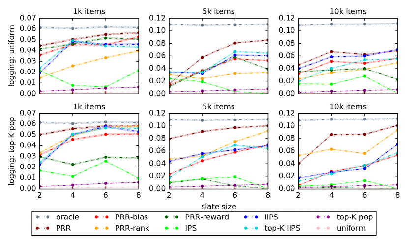
Figure 2: The reward (y-axis) of PRR and baselines in simulated A/B tests with varying slate sizes (x-axis), number of items (columns) and logging policies (rows). The shaded areas represent uncertainty and they are small since we run long A/B tests with $n_{\rm test}=100{\rm k}$.

4.2 Performance Comparison

We consider a realistic setting with relatively large catalogs and slates. The engagement features $\bm{y}$ are $5$-dimensional embeddings. The user interests $\bm{z}$ are $20$-dimensional binary vectors that encode the categories that are appealing to the user. The true parameters of the simulation sessions are randomly sampled from uniform distributions. In Fig. 2, we report the average A/B test reward of PRR with varying slate sizes, number of items and logging policies using 100k training samples. An interesting metric to assess the performance of algorithms is the ratio between their rewards and that of the oracle. We defer the plots of the relative performance to Fig. 3 in Appendix A. Overall, we observe that PRR outperforms the baselines across the different settings. Next we summarize the general trends of algorithms.

1. Varying logging policy: models that use the reward only, IPS and PRR-reward, favor uniform logging policies while those that use only the rank, IIPS and PRR-rank perform better with the top-K pop logging policy. PRR-bias discards the slate-level features $\bm{y}$ and uses a single parameter $\phi$ for all slates. Thus PRR-bias benefits from uniform logging policies as they allow learning $\phi$ that works well across all slates. Indeed, in Fig. 2 the gap between PRR and PRR-bias shrinks for the uniform logging policy. Finally, the performance of PRR is relatively stable for both logging policies.

2. Varying slate size: the performance of models that use the reward only, IPS and PRR-reward, deteriorates when the maximum slate size increases. On the other hand, those that use only the rank, IIPS and PRR-rank, benefit from larger slates as this leads to displaying more item comparisons. The addition of the top-K heuristic improves the performance of IIPS in some cases by spreading the mass over different items, making it not only focus on retrieving one but several high scoring items. However, the increase in performance is not always guaranteed which might be due to our choice of hyperparameters or our approximation of the marginal distributions of policies. Finally, PRR performs well across all slate sizes as it uses both the reward and rank.

3. Varying number of items: the models that use the rank benefit from large slates. Here we observe that the increase in performance is more significant for large catalogs. Also, the gap between the algorithms and the oracle becomes higher. In particular, models that use only the reward suffer a significant drop in performance when the number of items increases.

4.3 Speed Comparison

We assess the training speed of the algorithms with respect to the catalog and slate sizes $P$ and $K$. First, PRR and its variants compute $K+1$ scores $\theta_{0},\dots,\theta_{K}$ and normalize them using $Z=\sum_{\ell=0}^{K}\theta_{\ell}$. Therefore, evaluating PRR and its variants in one data-point costs roughly $\mathcal{O}(K)$, where we omit the cost of computing the scores since it is the same for all algorithms. In contrast, IPS and its variants compute a softmax over the catalog. This requires computing the normalization constant $\sum_{a^{\prime}\in[P]}\exp\{f_{\bm{\Xi}}(\bm{z})^{\top}\bm{\beta}_{a^{\prime}}\}$ in (12). Thus the evaluation cost of IPS and its variants is roughly $\mathcal{O}(P)$. This is very costly compared to $\mathcal{O}(K)$ in realistic settings where $P\gg K$. An additional consideration to compare the training speed of algorithms is whether they use successful slates only, which significantly reduces the size of training data. Taking this into account, the fastest of all algorithms is the PRR-rank since its evaluation speed is $\mathcal{O}(K)$ and it is trained on successful slates only. For instance, PRR-rank can be $\approx 20$ times faster to train than IPS as we show in Table 2.

Method	Evaluation Complexity	Statistical Efficiency	Training Time/Epoch
PRR	$\mathcal{O}(K)$	High	35
PRR-bias	$\mathcal{O}(K)$	Medium	33
PRR-rank	$\mathcal{O}(K)$	Medium	11
PRR-reward	$\mathcal{O}(K)$	Low	35
IPS	$\mathcal{O}(P)$	Low	230
IIPS	$\mathcal{O}(P)$	Medium	230
Top-K IIPS	$\mathcal{O}(P)$	Medium	230

Table 2: Properties of PRR and the baselines. The last column, Training Time/Epoch, corresponds to the training time per epoch in seconds for a simulated A/B test with 1M items, $n_{\rm train}=$100k, $K=8$ and batch size$=516$.

5 CONCLUSION

We present PRR, a scalable probabilistic model for personalized slate recommendation. PRR efficiently estimates the probability of a slate being successful by combining the reward and rank signals. It also optimizes the reward of the whole slate by distinguishing between slate-level and item-level features. Experiments attest that PRR outperforms competing baselines and it is scalable to large-scale tasks, for both training and decision-making. The shortcoming of our approach is that PRR is trained to predict the reward of any slate, while we only recommend the best one. There is a cost for this as PRR might require for example very high-dimensional embeddings, which can be costly for extremely low latency tasks. A possible path to improve this is to optimize a policy with small embeddings using the reward estimates of PRR instead of IPS.

Appendix A Additional Results

In Fig. 3, we report the ratio between the reward of the algorithms and that of the oracle.

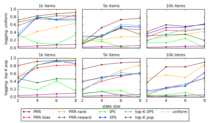
Figure 3: The ratio between the reward of the baselines and that of the oracle (y-axis) in simulated A/B tests with varying slate sizes (x-axis), number of items (columns) and logging policies (rows).

References

- Abbasifard et al. (2014) Mohammad Reza Abbasifard, Bijan Ghahremani, and Hassan Naderi. A survey on nearest neighbor search methods. International Journal of Computer Applications, 95(25), 2014.
- Aouali et al. (2021) Imad Aouali, Sergey Ivanov, Mike Gartrell, David Rohde, Flavian Vasile, Victor Zaytsev, and Diego Legrand. Combining reward and rank signals for slate recommendation, 2021. URL https://arxiv.org/abs/2107.12455.
- Aouali et al. (2022) Imad Aouali, Amine Benhalloum, Martin Bompaire, Benjamin Heymann, Olivier Jeunen, David Rohde, Otmane Sakhi, and Flavian Vasile. Offline evaluation of reward-optimizing recommender systems: The case of simulation, 2022. URL https://arxiv.org/abs/2209.08642.
- Ashkan & Clarke (2012) Azin Ashkan and Charles LA Clarke. Modeling browsing behavior for click analysis in sponsored search. In Proceedings of the 21st ACM international conference on Information and knowledge management, pp. 2015–2019, 2012.
- Bottou et al. (2013) Léon Bottou, Jonas Peters, Joaquin Quiñonero-Candela, Denis X Charles, D Max Chickering, Elon Portugaly, Dipankar Ray, Patrice Simard, and Ed Snelson. Counterfactual reasoning and learning systems: The example of computational advertising. Journal of Machine Learning Research, 14(11), 2013.
- Chapelle & Zhang (2009) Olivier Chapelle and Ya Zhang. A dynamic bayesian network click model for web search ranking. In Proceedings of the 18th international conference on World wide web, pp. 1–10, 2009.
- Chen et al. (2019) Minmin Chen, Alex Beutel, Paul Covington, Sagar Jain, Francois Belletti, and Ed H Chi. Top-k off-policy correction for a reinforce recommender system. In Proceedings of the Twelfth ACM International Conference on Web Search and Data Mining, pp. 456–464, 2019.
- Chuklin et al. (2013) Aleksandr Chuklin, Pavel Serdyukov, and Maarten De Rijke. Modeling clicks beyond the first result page. In Proceedings of the 22nd ACM international conference on Information & Knowledge Management, pp. 1217–1220, 2013.
- Chuklin et al. (2015) Aleksandr Chuklin, Ilya Markov, and Maarten de Rijke. Click models for web search. Synthesis lectures on information concepts, retrieval, and services, 7(3):1–115, 2015.
- Covington et al. (2016) Paul Covington, Jay Adams, and Emre Sargin. Deep neural networks for youtube recommendations. In Proceedings of the 10th ACM conference on recommender systems, pp. 191–198, 2016.
- Craswell et al. (2008) Nick Craswell, Onno Zoeter, Michael Taylor, and Bill Ramsey. An experimental comparison of click position-bias models. In Proceedings of the 2008 international conference on web search and data mining, pp. 87–94, 2008.
- Ding et al. (2019) Qin Ding, Hsiang-Fu Yu, and Cho-Jui Hsieh. A fast sampling algorithm for maximum inner product search. In The 22nd International Conference on Artificial Intelligence and Statistics, pp. 3004–3012. PMLR, 2019.
- Dudík et al. (2012) Miroslav Dudík, Dumitru Erhan, John Langford, and Lihong Li. Sample-efficient nonstationary policy evaluation for contextual bandits. In Proceedings of the Twenty-Eighth Conference on Uncertainty in Artificial Intelligence, UAI’12, pp. 247–254, Arlington, Virginia, USA, 2012. AUAI Press. ISBN 9780974903989.
- Dudík et al. (2014) Miroslav Dudík, Dumitru Erhan, John Langford, and Lihong Li. Doubly robust policy evaluation and optimization. Statistical Science, 29(4):485–511, 2014.
- Dupret & Piwowarski (2008) Georges E. Dupret and Benjamin Piwowarski. A user browsing model to predict search engine click data from past observations. SIGIR ’08, 2008.
- Garcin et al. (2014) F. Garcin, B. Faltings, O. Donatsch, A. Alazzawi, C. Bruttin, and A. Huber. Offline and Online Evaluation of News Recommender Systems at Swissinfo.Ch. In Proc. of the 8th ACM Conference on Recommender Systems, RecSys ’14, pp. 169–176, 2014.
- Gilotte et al. (2018) Alexandre Gilotte, Clément Calauzènes, Thomas Nedelec, Alexandre Abraham, and Simon Dollé. Offline a/b testing for recommender systems. In Proceedings of the Eleventh ACM International Conference on Web Search and Data Mining, pp. 198–206, 2018.
- Guo et al. (2009) Fan Guo, Chao Liu, and Yi Min Wang. Efficient multiple-click models in web search. In Proceedings of the Second ACM International Conference on Web Search and Data Mining, WSDM ’09, 2009.
- Hochreiter & Schmidhuber (1997) Sepp Hochreiter and Jürgen Schmidhuber. Long short-term memory. Neural Computation, 9(8):1735–1780, 1997.
- Horvitz & Thompson (1952) Daniel G Horvitz and Donovan J Thompson. A generalization of sampling without replacement from a finite universe. Journal of the American statistical Association, 47(260):663–685, 1952.
- Hu et al. (2011) Botao Hu, Yuchen Zhang, Weizhu Chen, Gang Wang, and Qiang Yang. Characterizing search intent diversity into click models. In Proceedings of the 20th international conference on World wide web, pp. 17–26, 2011.
- Huang et al. (2012) Jeff Huang, Ryen W White, Georg Buscher, and Kuansan Wang. Improving searcher models using mouse cursor activity. In Proceedings of the 35th international ACM SIGIR conference on Research and development in information retrieval, pp. 195–204, 2012.
- Ie et al. (2019) Eugene Ie, Vihan Jain, Jing Wang, Sanmit Narvekar, Ritesh Agarwal, Rui Wu, Heng-Tze Cheng, Tushar Chandra, and Craig Boutilier. Slateq: A tractable decomposition for reinforcement learning with recommendation sets. 2019.
- Jiang et al. (2019) Ray Jiang, Sven Gowal, Timothy A. Mann, and Danilo J. Rezende. Beyond greedy ranking: Slate optimization via list-cvae, 2019.
- Joachims et al. (2017) Thorsten Joachims, Laura Granka, Bing Pan, Helene Hembrooke, and Geri Gay. Accurately interpreting clickthrough data as implicit feedback. In Acm Sigir Forum, volume 51, pp. 4–11. Acm New York, NY, USA, 2017.
- Li et al. (2018) Shuai Li, Yasin Abbasi-Yadkori, Branislav Kveton, S Muthukrishnan, Vishwa Vinay, and Zheng Wen. Offline evaluation of ranking policies with click models. In Proceedings of the 24th ACM SIGKDD International Conference on Knowledge Discovery & Data Mining, pp. 1685–1694, 2018.
- Liu et al. (2014) Yiqun Liu, Chao Wang, Ke Zhou, Jianyun Nie, Min Zhang, and Shaoping Ma. From skimming to reading: A two-stage examination model for web search. In Proceedings of the 23rd ACM International Conference on Conference on Information and Knowledge Management, pp. 849–858, 2014.
- McInerney et al. (2020) James McInerney, Brian Brost, Praveen Chandar, Rishabh Mehrotra, and Benjamin Carterette. Counterfactual evaluation of slate recommendations with sequential reward interactions. In Proceedings of the 26th ACM SIGKDD International Conference on Knowledge Discovery & Data Mining, pp. 1779–1788, 2020.
- Sachdeva et al. (2020) Noveen Sachdeva, Yi Su, and Thorsten Joachims. Off-policy bandits with deficient support. In Proceedings of the 26th ACM SIGKDD International Conference on Knowledge Discovery & Data Mining, pp. 965–975, 2020.
- Swaminathan & Joachims (2015) Adith Swaminathan and Thorsten Joachims. Counterfactual risk minimization: Learning from logged bandit feedback. In International Conference on Machine Learning, pp. 814–823. PMLR, 2015.
- Swaminathan et al. (2017) Adith Swaminathan, Akshay Krishnamurthy, Alekh Agarwal, Miroslav Dudík, John Langford, Damien Jose, and Imed Zitouni. Off-policy evaluation for slate recommendation, 2017.
- Vaswani et al. (2017) Ashish Vaswani, Noam Shazeer, Niki Parmar, Jakob Uszkoreit, Llion Jones, Aidan N Gomez, Łukasz Kaiser, and Illia Polosukhin. Attention is all you need. Advances in neural information processing systems, 30, 2017.
- Wilhelm et al. (2018) Mark Wilhelm, Ajith Ramanathan, Alexander Bonomo, Sagar Jain, Ed H Chi, and Jennifer Gillenwater. Practical diversified recommendations on youtube with determinantal point processes. In Proceedings of the 27th ACM International Conference on Information and Knowledge Management, pp. 2165–2173, 2018.
- Yue et al. (2010) Yisong Yue, Rajan Patel, and Hein Roehrig. Beyond position bias: Examining result attractiveness as a source of presentation bias in clickthrough data. In Proceedings of the 19th International Conference on World Wide Web, WWW ’10, pp. 1011–1018, 2010.
- Zhang et al. (2011) Yuchen Zhang, Weizhu Chen, Dong Wang, and Qiang Yang. User-click modeling for understanding and predicting search-behavior. In Proceedings of the 17th ACM SIGKDD international conference on Knowledge discovery and data mining, pp. 1388–1396, 2011.
- Zhao et al. (2018) Xiangyu Zhao, Long Xia, Liang Zhang, Zhuoye Ding, Dawei Yin, and Jiliang Tang. Deep reinforcement learning for page-wise recommendations. In Proceedings of the 12th ACM Conference on Recommender Systems, pp. 95–103, 2018.