The Optical Appearance of Charged Four-Dimensional Gauss-Bonnet Black Hole with Strings Cloud and Non-Commutative Geometry Surrounded by Various Accretions Profiles

Abstract

Thanks for the releasing image of supermassive black holes (BHs) by the event horizon telescope (EHT) at the heart of the $M87$ galaxy. After the discovery of this mysterious object, scientists paid attention to exploring the BH shadow features under different gravitational backgrounds. In this scenario, we study the light rings and observational properties of BH shadow surrounded by different accretion flow models and then investigate the effect of model parameters on the observational display and space-time structure of BHs in the framework of our considering system. Under the incompatible configuration of the emission profiles, the images of BHs comprise that the observed luminosity is mainly determined by direct emission, while the lensing ring will provide a small contribution of the total observed flux and the photon ring makes a negligible contribution due to its exponential narrowness. More importantly, the observed regions and specific intensities of all emission profiles are changed correspondingly under variations of parameters. For optically thin accreting matters, we analyze the profile and specific intensity of the shadows with static and infalling accretions models, respectively. We find that with an infalling motion the interior region of the shadows will be darker than in a static case, due to the Doppler effect of the infalling movement. Finally, it is concluded that these findings support that the change of BH state parameters will change the way of space-time geometry, thus affecting the BH shadows dynamics.

I Introduction

A black hole is a mysterious region of space-time, where the gravitational force is extremely intense that nothing, no particles, or even electromagnetic radiation such as light, can escape from it. A BH can be formed at the final stage of a massive star. When such a star has completely exhausted the nuclear fuel in its core at the end of its life cycle, the core becomes unbalanced and gravitational collapse occurs inside the core, and the outer layers of the star are blown away. After this, the massless weight of constituent matter falls in the dying sphere to a point of zero volume and infinite density, so-called singularity. The simplest model for BH formation involves a collapsing thin spherical shell of massless matter, i.e., a shell of photons, gravitons, or massless neutrinos with very small radial extension and total energy. In general relativity (GR), BH is one of the most fascinating predictions, and researchers have been trying to resolve this mysterious puzzle. The Laser-Interferometer Gravitational Wave-Observatory (LIGO) detects the emission of gravitational waves from BHs merger 1 .

In 2019, the EHT captured the first evidence for the existence of ultra-high angular resolution image of accretion flows around a super-massive object at the center of $M87$ ($M=6.5\pm 0.7\times 10^{9}M_{\odot}$) galaxy 2 ; 3 ; 4 ; 5 ; 6 ; 7 . The canonical interpretation of the $M87$ galaxy shows that the gravitational field of a BH contains a photon sphere when generally illuminated by an thin accretion matter. The interior of dark region is bounded by a bright band, known as the BH shadow and photon sphere, respectively. The existence of a strong gravitational interaction at the core of BH regimens makes the gravitational deflection of light, which provide a comprehensive way to analyze the BH shadow. Therefore, the analysis of BH shadow and gravitational lensed may provide the feasible way to evaluate the strength of the gravitational field in space-time geometry and support the prediction of Einstein’s GR 8 ; 9 ; 10 ; 11 .

The intensity of emitted light depends upon the location of the distant observer, leading to a dark inner region and intense photon ring. Generally, the shadow of different BHs has been discussed in the literature and tries to find a complex pattern of several light ray trajectories around a dark thin disk. The study of light deflection by a compact star or BH was initially studied in 9 . Later, the extension of BH thin accretion disk and critical curve observed the image of BH in 11 . Theoretically, the critical curve is the light trajectory traced backward from the distant viewer, which would have asymptotically approach towards a bound photon ring. For the Schwarzschild BH, the value of bound photon ring is $r=3M$, (where $M$ is the mass of BH) and the radius of the critical impact parameter curve is $b=3\sqrt{3}M$.

However, the region of impact parameter depends on the geometrical interpretation and various physical properties of the illuminating accretion flow of BHs 12 . In addition, the width and the intensity of lensing rings is changed with the variation of emission region and size of the shadow dependent on the emission model, the accretion has a minor effect on the dark central region 13 . The influence of quintessence dark energy dynamics on the shadow of BH and thin accretions disk surrounded by various trajectories of light are widely discussed in 14 . Further, the authors in 14 concluded that the existence of a cosmological horizon plays an significant part in the BH shadows and the location of photon rings for both stationary and infalling accretions are lie in the same orbit. Shadows and photon rings with the static and spherical infalling accretions are analyzed in the framework of four-dimensional Gauss-Bonnet (GB) BH, and the influence of the GB coupling constant on the BH shadow and dynamics of photon spheres have been calculated in 15 .

In the background of Einstein GB-Maxwell gravity, Ma et al. 16 studied the spherically symmetric charged BH shadow and its photons sphere with the sequence of inequalities of the BH horizon and its mass. Gao et al. 17 discussed gravitational lensing of a hairy BH in Einstein-Scalar-GB gravity and compared the consistency of BH shadow with EHT data. Guo et al. 18 considered the perfect fluid within Rastall gravity and investigated the shadow and photon sphere of charged BH with infalling accretion and obtained brighter photon sphere luminosity than the static spherical accretion. The luminosity of shadows and light rings of the Hayward charge BH are affected by the accretion flow property is a result obtained in 19 . The analysis of BH shadow in GR as well as in extended gravitational theories provides a new way to discover the properties of BHs 20 ; 21 ; 22 ; 23 ; 24 ; 25 ; 26 ; 27 .

The idea of the non-commutative (NC) geometry is extensively used to evaluate the BH solutions, wormhole geometry, and cosmological constraints. Recently, NC geometry has obtained a significant attraction as it provides an comprehensive way to analysis the effects of quantum gravity in space-time structure f1 ; f2 . For instance, the influence of NC operators on BH is a interesting subject, and a number of methods are being proposed to explore the NC geometry f3 ; f4 ; f5 . This geometry can be implemented to GR by modifying the matter source, considering the minimal length instead of the Dirac function, replaced by Gaussian distribution or Lorentzian distribution 29 . Regarding the growing interest of researchers in further analysis of BH shadows, we have proposed a new approach to discussing the observational characteristics of BH space-time. In the present manuscript, we investigate the shadow of four-dimensional GB charged BH with spherical accretions under the influence of a cloud of strings and NC geometry 27 ; 28 ; 29 . Particularly, we study the qualitative features of BH shadows under the influence of charge, the cloud of strings, and NC geometry parameters. In Sec. II, we provide the basic formulation of our considering system and studied the effective potential corresponding to the light trajectories. Section III is dedicated to the optical appearance of photon rings with thin disk accretion flow models and to studying the shadow with specifically observed intensities. The analysis of shadows and photon spheres rings with a static accretion matter is dealt with in Sec. IV. In next section, we discuss the dynamics of the BH accretion with infalling matters. The last section is devoted to the conclusion and discussion of the current analysis.

II Light Deflection in the Charged GB BH with Cloud of Strings and NC Geometry

The Einstein-Hilbert action of GB gravity is formulated as 15

$$\mathcal{I}=\frac{1}{16\pi G}\int d^{4}{x\sqrt{-g}}[R+\alpha(R_{\gamma\delta\zeta\xi}R^{\gamma\delta\zeta\xi}-4R_{\gamma\delta}R^{\gamma\delta}+R^{2})],$$ (1)

where $R$ is the curvature scalar, by re-scaling the GB coupling constant $\alpha$, i.e., $\alpha$/$D-4$ and taking the limit $D\rightarrow 4$ in the GB term, one can obtain the solution of four-dimensional GB BH 30 . We consider the static and spherically symmetric metric for four-dimensional GB BH 28

$$ds^{2}=-f(r)dt^{2}+\frac{dr^{2}}{f(r)}+r^{2}d\theta^{2}+r^{2}\sin^{2}\theta d\varphi^{2},$$ (2)

with

$$f(r)=1+\frac{r^{2}}{2\alpha}\bigg{(}1-\sqrt{1+4\alpha\big{(}\frac{2M}{r^{3}}-\frac{Q}{r^{4}}+\frac{a}{r^{2}}\big{)}}\bigg{)}.$$ (3)

The solution (3) can be characterized by the GB coupling constant $\alpha$, mass $M$, Charge $Q$ and cloud of string parameter $a$, which is consider to be positive.

The point-like structure with smeared objects, the mass density of a static and spherically symmetric gravitational source is given by Lorentzian distribution as follows 29

$$\rho_{\phi}=\frac{\sqrt{\phi}M}{\pi^{3/2}(\pi\phi+r^{2})^{2}},$$ (4)

where $\phi$ is the strength of NC parameter in Lorentzian distribution. The smeared mass of matter distribution can be obtain as 27

$$\mathcal{M_{\phi}} = \int^{r}_{0}4\pi r^{2}\rho_{\phi}(r)dr=\frac{2M}{\pi}\bigg{[}\arctan\big{(}\frac{r}{\sqrt{\pi\phi}}\big{)}-\frac{r\sqrt{\pi\phi}}{\pi\phi+r^{2}}\bigg{]},$$ (5)

$$= M-\frac{4\sqrt{\phi}M}{\sqrt{\pi}r}+\mathcal{O}(\phi^{3/2}).$$

In this way, the equation (3) can be rewritten as

$$f(r)=1+\frac{r^{2}}{2\alpha}\bigg{(}1-\sqrt{1+4\alpha\big{(}\frac{2\mathcal{M}_{\phi}}{r^{3}}-\frac{Q}{r^{4}}+\frac{a}{r^{2}}\big{)}}\bigg{)},$$ (6)

which modify the NC BH geometry as

$$f(r)=1+\frac{r^{2}}{2\alpha}\bigg{(}1-\sqrt{1+4\alpha\big{(}\frac{2M}{r^{3}}-\frac{8\sqrt{\phi}M}{\sqrt{\pi}r^{4}}-\frac{Q}{r^{4}}+\frac{a}{r^{2}}\big{)}}\bigg{)}.$$ (7)

In order to found the location of horizons, one can solve the equation $f(r)=0$, and following two analytic solutions are obtained

$$r_{h} = \frac{M\pi^{1/4}+\sqrt{\sqrt{\pi}(M^{2}+(a-1)((Q+\alpha)+8M\sqrt{\phi}))}}{(1-a)\pi^{1/4}},$$ (8)

$$r_{c} = \frac{M\pi^{1/4}-\sqrt{\sqrt{\pi}(M^{2}+(a-1)((Q+\alpha)+8M\sqrt{\phi}))}}{(1-a)\pi^{1/4}},$$ (9)

where $r_{h}$ and $r_{c}$ correspond to the event horizon and cosmological horizon of the BH, respectively. For the existence of a horizon, the GB coupling parameter $\alpha$ should fall in the allowed range $-8\leq\alpha/M\leq 1$. For $\alpha>0$, we have two horizons, while for $\alpha<0$, only one horizon exists. Although $\alpha>0$ depicts the properties of the inverse string tension, the solution (3) also allows the case $\alpha<0$. So, we expect some interesting aspects of GB gravity as it was argued in 30 .

To analysis the accretion flow of photons spheres around the BH, we need to analyze the behavior of light deflection in geometrical optics near the BH shadow. The geodesic motion can be encapsulated with the help of the Euler-Lagrange equation, can be written in the following form

$$\frac{d}{d\eta}\bigg{(}\frac{\partial\mathcal{L}}{\partial\dot{x}^{\alpha}}\bigg{)}=\frac{\partial\mathcal{L}}{\partial x^{\alpha}},$$ (10)

in which $\eta$ is the affine parameter, $\dot{x}^{\alpha}$ is the four-velocity of BH light rays, “.” represents the derivative with respect to $\eta$. The Lagrangian $(\mathcal{L})$ of photons can be written as:

$$\mathcal{L}=\frac{1}{2}g_{\alpha\beta}\dot{x}^{\alpha}\dot{x}^{\beta}=\frac{1}{2}\bigg{(}-f(r)\dot{t}^{2}+\frac{\dot{r}^{2}}{f(r)}+r^{2}\dot{\theta}^{2}+r^{2}\sin^{2}\theta\dot{\varphi}^{2}\bigg{)}.$$ (11)

The spherical symmetry allows us to choose the motion of photons on the equatorial plane with $\theta=\pi/2$ and $\dot{\theta}=0$ without loss of generality 10 ; 31 . From (2), the metric coefficients are independent of time $t$, and the azimuthal angle $\varphi$. So, two conserved quantities can be evaluated such as energy $E=\partial\mathcal{L}/\partial\dot{t}=f(r)\dot{t}$, and angular momentum of photon $\mathcal{J}=\partial\mathcal{L}/\partial\dot{\varphi}=r^{2}\dot{\varphi}$. Using Eqs. (7), (10) and (11), we obtain

$$\dot{t}=\frac{1}{b\bigg{(}1+\frac{r^{2}}{2\alpha}\bigg{(}1-\sqrt{1+4\alpha\big{(}\frac{2M}{r^{3}}-\frac{8\sqrt{\phi}M}{\sqrt{\pi}r^{4}}-\frac{Q}{r^{4}}+\frac{a}{r^{2}}\big{)}}\bigg{)}\bigg{)}},$$ (12)

$$\dot{\varphi}=\pm\frac{1}{r^{2}},$$ (13)

$$\dot{r^{2}}+\frac{1}{r^{2}}\bigg{(}1+\frac{r^{2}}{2\alpha}\bigg{(}1-\sqrt{1+4\alpha\big{(}\frac{2M}{r^{3}}-\frac{8\sqrt{\phi}M}{\sqrt{\pi}r^{4}}-\frac{Q}{r^{4}}+\frac{a}{r^{2}}\big{)}}\bigg{)}\bigg{)}=\frac{1}{b^{2}},$$ (14)

where $``+"$ and $``-"$ in Eq. (13) corresponds to the anti-clockwise/clockwise motion of photon, respectively. Further, we define the affine parameter $\eta$, by $\frac{\eta}{\mathcal{J}}$ and the impact parameter $b_{c}=\frac{\mathcal{J}}{E}$, which is used to evaluate the vertical distance between the two lines, such as geodesic and parallel lines having the same origin. Equation (14) is used to evaluate the geodesic equation in the form of the effective potential, one can write as

$$\dot{r^{2}}+V_{e}(r)=\frac{1}{b^{2}},$$ (15)

where

$$V_{e}(r)=\frac{1}{r^{2}}\big{(}f(r)\big{)}.$$ (16)

In the equatorial plane, the null geodesic exists in space-time region and the light rays projected on the equatorial plane, yielding a circular orbit. The position of the maximum effective potential correspond to the frequency of threshold stability for the null geodesic circular geometry around $b_{c}$ having a critical curve. The photon will move around the BH in an unbalanced circular orbit, at this time, the surface of the photon sphere corresponds to the surface of the circular orbit. The motion of the light rays on the photon sphere should satisfy the conditions $\dot{r}=0$ and $\ddot{r}=0$. Further, the motion of photon sphere orbit can be translated as

$$V_{e}(r)=\frac{1}{b^{2}},\quad V^{\prime}_{e}(r)=0,$$ (17)

where prime represent the derivative with respect to $r$. Based on this equation, the shadow radius of photon sphere $r_{p}$, impact parameter of the critical curve $b_{c}$ and radii of event horizon $r_{h}$ are obtained for different values of model parameters and listed in Table. 1. The quantities $r_{p}$ and $b_{c}$ are satisfying the following equations:

$$r^{2}_{p}=b^{2}_{c}f(r),\quad 2b^{2}_{c}f(r)^{2}-r^{3}_{p}f^{\prime}(r)=0.$$ (18)

Due to the correlation of parameters, the geometry of space-time varies with the variation of parameters, which means that the trajectories of photons will be different corresponding to different numerical values. For instant, we choose fixed values of charge $Q$ and NC parameter $\phi$ and evaluate the event horizon $r_{h}$, critical curve $b_{c}$ and radius of photon sphere $r_{p}$, for different values of coupling constant $\alpha$ and cloud of strings parameter $a$. Similarly, we can also evaluate the numerical values of $r_{h}$, $b_{c}$ and $r_{p}$ corresponding to different values $Q$ and $\phi$ by fixing other parameters.

One can see from Table. 1, the numerical values of $r_{h}$ , $b_{c}$ and $r_{p}$ decreases with an increase in the values of $\alpha$. On the other hand, these values increase directly with increasing values of $a$. Hence, it implies that the BH photon ring shrinks inward as one increases the values of $\alpha$ and expands outward concerning $a$. Taking some fixed values of the parameters, we depict the effective potential $V_{e}(r)$, in Fig. 1 (left panel). Let us consider Fig. 1 (left panel), there is no effective potential at the event horizon. The trajectory of effective potential increases maximum in the position of the photon sphere and then vanishes gradually with the increment of radius $r$.

$\alpha$	$-7.55$	$-5.55$	$-2.55$	$0.22$	$0.44$	$0.55$
$r_{h}$	$4.11292$	$3.71661$	$2.96995$	$1.72553$	$1.47589$	$1.21524$
$b_{c}$	$7.70838$	$7.31300$	$6.55952$	$5.37765$	$5.20921$	$5.11003$
$r_{p}$	$5.01684$	$4.64989$	$3.94120$	$2.75860$	$2.56800$	$2.44825$
$a$	$0.1$	$0.2$	$0.3$	$0.4$	$0.5$	$0.6$
$r_{h}$	$1.61637$	$1.92883$	$2.13273$	$2.81072$	$3.49576$	$4.51162$
$b_{c}$	$5.29741$	$6.42990$	$7.98517$	$10.22250$	$13.64610$	$19.36120$
$r_{p}$	$2.66938$	$3.10145$	$3.64973$	$4.37446$	$5.38328$	$6.89082$

Table 1: The numerical values of involved physical quantities for various values of $\alpha$ and $a$ for fixed values of $Q=0.1$ and $\phi=0.01$ with $M=1$.

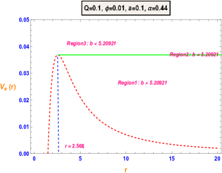
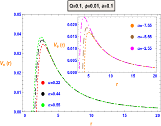
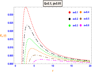
Figure 1: The Behaviour of $V_{e}(r)$ versus $r$ for some specific values of model parameters (left panel), for different $\alpha$ (middle panel) and for different $a$ (right panel) with $M=1$. In left panel, dashed blue line indicates the radius of photon sphere $r_{p}$ while green line corresponds to $V_{e}(r)=1/b_{c}^{2}$.

In region $1$ ($b>b_{c}$), the light rays hit the potential barrier which is generated due to $V_{e}(r)$, region $2$ ($b=b_{c}$) defines the behavior of impact parameter which is nearest to the photon sphere radius and rotate around the BH, and region $3$ ($b<b_{c}$), light fall into BH because there is no encounter the potential barrier. The changing trend of the effective potential for different values of $\alpha$ and $a$ are presented in Fig. 1 (middle and right panels). To depict the geodesics of photons, using Eqs. (13) and (15) with the setting of $u_{0}=1/r$ as

$$\Psi(u_{0})=\frac{du_{0}}{d\varphi}=\bigg{(}\frac{1}{b^{2}}-u_{0}^{2}\bigg{(}1+\big{(}1-\big{(}1+4\alpha(au_{0}^{2}+2Mu_{0}^{3}-Qu_{0}^{4}-(8Mu_{0}^{4}\sqrt{\phi})/\sqrt{\pi})\big{)}^{\frac{1}{2}}\big{)}/2u_{0}^{2}\alpha\bigg{)}\bigg{)}^{\frac{1}{2}}.$$ (19)

The optical appearance of the BH shadow depends on Eq. (19), and we plot the ingoing or outgoing trajectories through the ray-tracing procedure as presented in Figs. 2 and 3. The light deflection for the region $b<b_{c}$ (orange lines), the light rays fall into BH. For case, $b=b_{c}$ (green lines), locate the position of the photon sphere and revolve around the BH whereas for $b>b_{c}$ (blue lines), the light ray deflected and move towards the BH from an infinite location to one closest point and moves away from BH to infinity.

In addition, regions $1$, $2$ and $3$ are presented in Fig. 1 (left panel) correspond to the blue, green, and orange lines in Figs. 2 and 3 in general sense. We plot Figs. 2 and 3 for some specific choices of model parameters and find the shadow image of BH in space-time which is different for each set of these values.

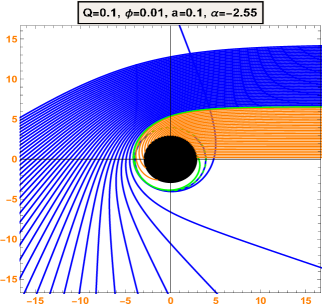
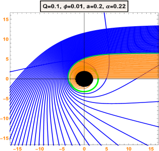
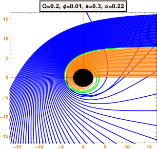
Figure 2: The trajectories of photon rings for different parameters in polar coordinates $(r,\varphi)$. The considering BH is shown as solid black disks, and the blue, green and orange lines correspond to $b>b_{c}$, $b=b_{c}$ and $b<b_{c}$ regions, respectively. The dashed green line represents the radius of photon sphere and the mass of BH as $M=1$.

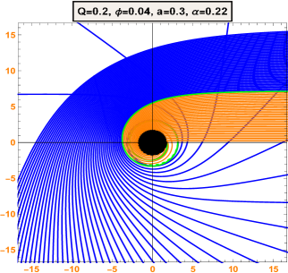
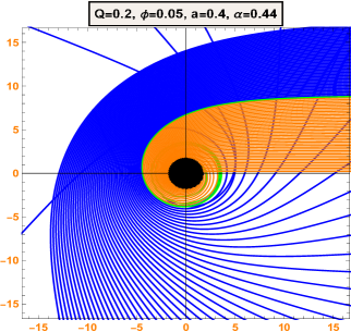
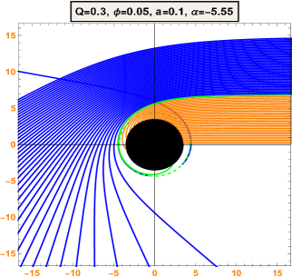
Figure 3: The trajectories of photon rings for different parameters in polar coordinates $(r,\varphi)$. The considering BH is shown as solid black disks, and the blue, green and orange lines correspond to $b>b_{c}$, $b=b_{c}$ and $b<b_{c}$ regions, respectively. The dashed green line represents the radius of photon sphere and the mass of BH as $M=1$

III Shadows and Photon Rings with Thin-Accretion Flow Models

Now, we are going to discuss the optical appearance of thin disk accretion around the BH in NC geometry with the cloud of strings and charge in the background of four-dimensional GB BH. Our focus is to investigate the photon rings and lensing rings surrounding the BH shadow and observed the light intensity by the thin accretion disk.

III.1 Direct Emission, Lensing Emission and Photon Ring Emission

To differentiate the photon ring and lensing ring near the BH, one can define the total number of light trajectories by $n(b)=\varphi/2\pi$, where $\varphi$ represents the total change in azimuthal angle beyond the horizon 12 . The optical appearance depends upon how near the impact parameter $b$, to its critical curve $b_{c}$. According to 12 , the trajectories of photon orbits are mainly divided into three cases and depending upon the number of orbits around the BH solution such as, $n<3/4$ corresponds to direct emission, the light trajectories crossing the equatorial plane just once, while the lensing ring corresponds to $3/4<n<5/4$, the light trajectories crossing the equatorial plane at leat $2$ times and when $n>5/4$ it corresponds to photon ring, the light trajectories crossing the equatorial plane minimum $3$ times.

From Fig. 4, one can see the that classify regions of direct, lensing and photon ring emissions for each set of parameters. We take different values of parameters for each set for example, set $1$, $2$ and $3$ correspond to $Q=0.3,\phi=0.05,a=0.1,\alpha=-5.55$, $Q=0.1,\phi=0.01,a=0.1,\alpha=-2.55$ and $Q=0.2,\phi=0.01,a=0.2,\alpha=0.22$, respectively. The intervals of $b$ which is related to numerical regions of emissions are listed as

$$\text{Set}:1\begin{cases}&\text{Direct emission: $n<3/4,b<6.78545$ and $b>8.13506$},\\ &\text{Lensing ring: $3/4<n<5/4$, $6.78545<b<6.8203$ and}\\ &\text{$6.82030<b<8.13506$},\\ &\text{Photon ring: $n>5/4$, $6.82737<b<6.83069$},\end{cases}$$

$$\text{Set}:2\begin{cases}&\text{Direct emission: $n<3/4,b<6.48387$ and $b>7.64494$},\\ &\text{Lensing ring: $3/4<n<5/4$, $6.48387<b<6.55920$ and}\\ &\text{$6.57435<b<7.59970$},\\ &\text{Photon ring: $n>5/4$, $6.55920<b<6.57435$},\end{cases}$$

$$\text{Set}:3\begin{cases}&\text{Direct emission: $n<3/4,b<5.85057$ and $b>8.98695$},\\ &\text{Lensing ring: $3/4<n<5/4$, $5.85057<b<6.333309$ and}\\ &\text{$6.51403<b<8.98695$},\\ &\text{Photon ring: $n>5/4$, $6.33330<b<6.51403$},\end{cases}$$

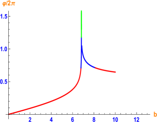
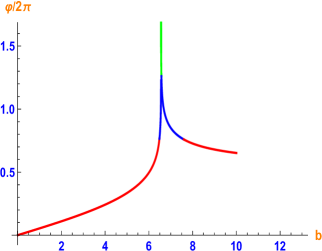
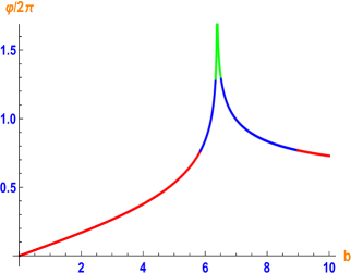
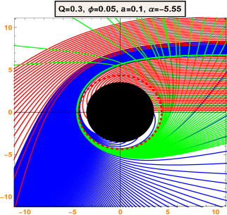
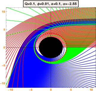
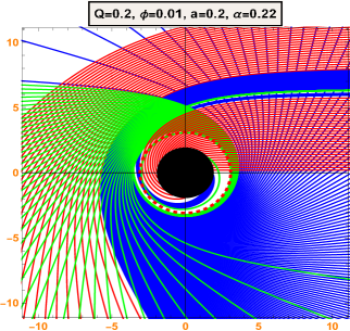
Figure 4: The relationship between different trajectories of photons and impact parameter $b$, for specific values of model parameters in polar coordinates $(r,\varphi)$. Here, the spacings of $b$ are $1/5$, $1/100$ and $1/1000$ for direct emission, lensing and photon ring corresponds to red, blue and green trajectories, respectively. The BH is shown as solid black disk and dashed red line represents the photon orbit and the mass of BH as $M=1$.

It is worth mentioning that the physical interpretation of photon behavior around the BH is different for each set. With the variation of numerical values, the radius of BH is gradually varying and hence, the bands of photon, lensing, and direct emissions are also changing the brightness and path of trajectories.

III.2 Observational Appearance and Transfer Functions

Now, we are going to analysis the profile of a BH with an optically/geometrically thin disk accretion and to observe the specific intensity. We consider that the disk is in the rest frame of static world-lines, and the emission of photons from it should obey the fundamental features of isotropy. In addition, as argue in 12 , we consider that the viewer is static and located at the zone of north pole and ignored the influence of other lights emitted from different sources in space-time and only focus on the light intensity which is emitted from a thin disk.

In this scenario, we delegate the specific emitted intensity and frequency of the accretion disk as $I_{\text{e}}(r)$ and $\nu_{\text{e}}$, where observed specific intensity and frequency are denoted as $I_{\text{obs}}(r)$ and $\nu$. Using the fact of Liouville’s theorem, the quantity $I_{\text{e}}(r)/\nu_{\text{e}}^{3}$ is conserved in the direction of light propagation and hence the observed specific intensity can be defined as

$$I_{\text{obs}}(r)=f(r)^{\frac{3}{2}}I_{\text{e}}(r).$$ (20)

The total observed intensity is deduced by integration over the entire range of different frequencies as

$$I=\int I_{\text{obs}}(r)d\nu=\int f(r)^{2}I_{\text{e}}d\nu_{\text{e}}=f(r)^{2}I_{\text{em}}(r),$$ (21)

where $I_{\text{em}}(r)=\int I_{\text{e}}d\nu_{\text{e}}$ is the total emitted radiation intensity near the thin accretion. From the previous discussion, if any photon light ray traced backwards from the observers screen passes through the thin disk accretion plane once (see blue and green lines from Fig. 4), it will get more light rings from the emission disk .

Hence, the total received optical luminosity will be the sum of all the intensities from each intersection, mathematically defined as $I(r)=\sum\limits_{\begin{subarray}{c}p\end{subarray}}f(r)^{2}I_{\text{em}}|_{r}=r_{p}(b)$, where $r_{p}(b)$ is called the transfer function, containing the information about the radial position of the $p^{th}$ intersection between the light with the impact parameter $b$ and the disk. Moreover, the slope of the transfer $dr/db$, represents the demagnification factor of the image 14 . In Fig. 5, the red line corresponds to the direct emission and represents the first transfer function for $p=1$. Since the profile of the direct image is the red-shift source profile therefore its slope is almost equal to unity.

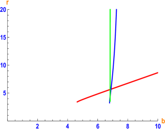
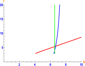
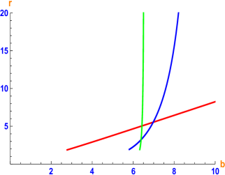
Figure 5: The profile depicts the first three transfer functions of the BH under different values of parameters. Here, we plot left to right panels with the values of set $1$, $2$ and $3$, respectively and the mass of BH as $M=1$.

The blue line corresponds to the lensing ring and represents the second transfer function for $p=2$. Here, the impact parameter $b$, is closed to the critical curve $b\sim b_{c}$. One can see that as the value (behaviour) of impact parameter $b$ increases, the slope of the second transfer function also increases, and hence, the back side appearance of the thin disk will be (de)magnified due to its large slope. The green line corresponds to the photon ring and represents the third transfer function for $p=3$. The slope $dr/dp$ is closed to $\infty$ so, the appearance of the front side of the thin disk will be highly demagnified. Further, we ignored the later transfer functions safely because the image depicted from these transfer functions is extremely (de)magnified and negligible.

III.3 Specific Luminosities of Thin Accretion Disks

Now, we consider an optically and geometrically thin disk model to observe the further specific intensity surrounding our BH solution on the equatorial plane. (Actually, this type of model evaluate the accretion matters when the accretion flow velocities is sub-Eddington with large opaque but ignores those with high accretion velocities and mass 32 . For instance, around the supermassive BHs, the accretion disk may effectively turn into an apparently thin but structurally thick one 33 ). The main source of observed specific light intensity is a thin disk and its luminosity only depends upon the radial coordinate $r$. So, we assume the following three toy models which is used to evaluate the realistic cases of thin matters.

• Model $1$: We assume that the matter emission begins from the peak point of the radius at the inner-most stable circular orbit (isco) for time-like observers. Therefore, we consider the model for this emission profile is a decay function, which is defined as

  $$I^{1}_{\text{em}}(r)=\begin{cases}\text{$(\frac{1}{r-(r_{\text{isco}}-1)})^{2},$ \quad if $r>r_{\text{isco}}$}\\ \text{$0$,\quad\quad\quad\quad\quad\quad if $r\leq r_{\text{isco}}$}\end{cases}$$ (22)

  

  

  

  

  

  

  

  

  

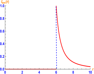
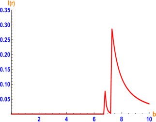
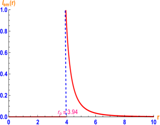
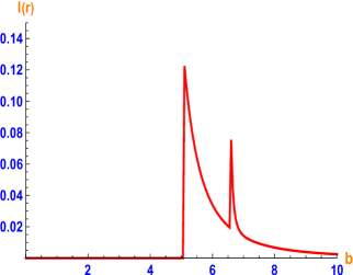
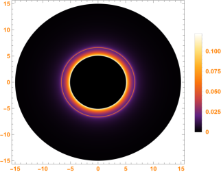
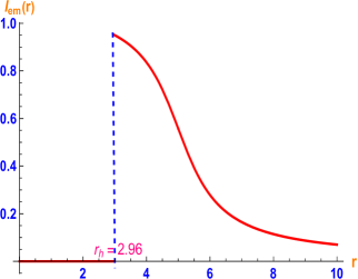
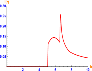
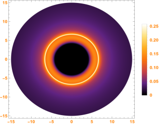
  Figure 6: Optical observation of thin disk accretion near the BH with different emission matter profiles, viewed from a face-on orientation. From left to right panels, the depicted graphs are reflecting the various emissions, observed emission and two dimensional optical appearance, respectively. The numerical values of parameters for all profiles are defined in set $2$ and the mass of BH as $M=1$.

• Model $2$: the considering emission has a sharp spikes at the isco location, having relatively similar center and asymptotic dynamics as model $1$. But the emission luminosity attenuation is significantly larger, so that the emission has decay characteristics of the third-order, mathematically defined as

  $$I^{2}_{\text{em}}(r)=\begin{cases}\text{$(\frac{1}{r-(r_{p}-1)})^{3},$ \quad if $r>r_{p}$}\\ \text{$0$,\quad\quad\quad\quad\quad if $r\leq r_{p}$}\end{cases}$$ (23)

• Model $3$: This emission lie beyond the horizon $r_{h}$, but its decaying rate is moderate than the previous two cases, as defined below

  $$I^{3}_{\text{em}}(r)=\begin{cases}\text{$\frac{\frac{\pi}{2}-\arctan(r-5)}{\frac{\pi}{2}-\arctan(-3)},$ \quad if $r>r_{h}$}\\ \text{$0$,\quad\quad\quad\quad\quad if $r\leq r_{h}$}\end{cases}$$ (24)

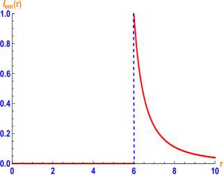
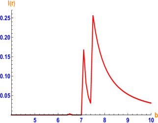
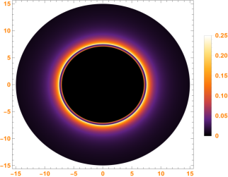
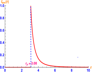
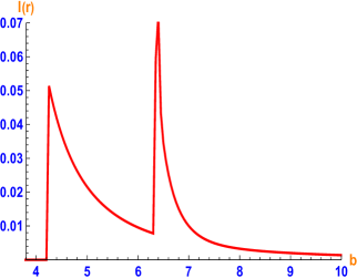
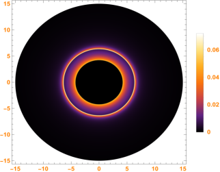
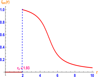
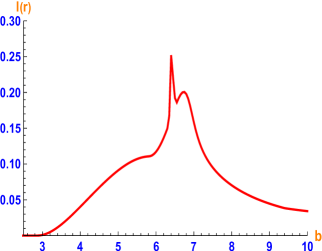
Figure 7: Optical observation of thin disk accretion near the BH with different emission matter profiles, viewed from a face-on orientation. From left to right panels, the depicted graphs are reflecting the various emissions, observed emission and two dimensional optical appearance, respectively. The numerical values of parameters for all profiles are defined in set $3$ and the mass of BH as $M=1$.

With the help of previously defined toy models, we consider just two examples for different numerical values of parameters as defined in Figs. 6 and 7, and showed the results of intensity and analyzed the emission under these constraints. In Figs. 6 and 7, the left column shows the emission profile from the accretion has good behavior outside the photon sphere and defines a connection between specific emission intensity and the radial coordinate $r$. The middle column depicts the one dimensional (observed intensity) function of $I(r)$, which is related to $b$, where as the right column is the two dimensional density profiles that reflect the optical appearance of observed intensities.

From Fig. 6 (first row, left panel), we observed that the emission flow has reached its peak value, close to the critical case of the impact parameter $r\sim b$, after that decaying dramatically to zero with the increasing values of $r$. In the middle panel, due to the intensity of gravitational lensing, we see that there are two spikes separated the photon and lensing orbit independently, and the corresponding observed image decays similar to $b>7.48M$. However, the confined region of the lensing ring lies in the range $6.85M<b<7.34M$, providing only a small contribution to the total flux while the photon ring contribute the negligible luminosity. Therefore, one needs to see the main contribution in the observed (optical) appearance which is obtained from the direct emission and yields a wide rim while lensing ring makes a small contribution, and we find it inner of a wide rim. Moreover, the innermost region represents the photon ring contribution to the total flux which is difficult to detect in the right panel of density profiles and spikes at $b\sim 6.64M$.

From the second row of Fig. 6, the emission attained a peak value near the photon sphere at $r_{p}=3.94$ as shown in the left panel. The view of the middle panel reflects that the direct emission intensity shows the maximum value at $b=5.11$ and then shows a nice fluctuating behavior with an increase of $b$. Further, the region of lensing ring makes a significant intensity in the wide range of $b$ lie in $6.55M<b<6.83M$, while the photon ring emission has a narrower the spike at $b\sim 6.64M$ which can hardly be differentiated from the lensing one which leads to highly demagnetized to a narrow region and the intensity of the direct emission is still observed dominant. The overall results in the two dimensional optical appearance is visualized in the right panel. The lensing ring has small contribution to the total brightness while the photon ring is hardly diluted and narrowly visible.

Finally, in the third row of Fig. 6, the emitted region has been increased to the event horizon $r_{h}=2.96$, as shown in the left column and the decay rate of the emission is very moderate as compared to previous two models. One can see that from the inner rim, the observed intensity lies in the lensed position of the event horizon at $b\sim 0.25M$. The observational intensity increases suddenly and reaches at highest point in the emission of the photon ring and lies beyond the dark region due to the influence of gravitational red-shift. After this, the observed intensity start to show decaying behaviour nicely at $b\sim 6.64M$ in the photon ring and the participation of the lensing ring to the total flux is appreciable as compared to previous two cases. In this case, the observed appearance reflect a narrow but makes a prominent brighter extended ring contribution to the observed intensity, but the photon ring is still safely ignored.

From Fig. 6, it is interesting to mention that the dark interior regions are different for different plots of emissions, but the location of the photon ring stays always at $b\sim 6.64M$. In addition, we plot all the emission profiles and observed intensities in Fig. 7. The graphical description is the same for these profiles as we discussed in Fig. 6. The differences are the location of the photon/lensing rings and the quantities of luminosity intensities. The optical appearance in these flow models is physically well behave and viable with the statistical mechanics obtained from the original analysis of the Schwarzschild BH as discussed in 12 .

IV Shadows of the BH with Rest Spherical Accretion

Here, we are going to analyze the shadows of the BH with static spherical accretion model for various values of model parameters. We investigate the shadow of charged four-dimensional GB BH with the influence of NC parameter and cloud of strings for static spherical accretion. To this end, we focus on the observed specific intensity (which is usually defined in $\text{ergs}^{-1}\text{cm}^{-2}\text{str}^{-1}\text{Hz}^{-1}$), as expressed in 34 ; 35 .

$$I^{\text{obs}}(b)=\int g^{\text{obs}3}j(\nu^{\text{obs}}_{e})dl_{p},$$ (25)

where $g^{\text{obs}}=\nu^{\text{obs}}_{o}/\nu^{\text{obs}}_{e}$ is the red-shift factor, $\nu^{\text{obs}}_{o}$ is the observed photon frequency, $\nu^{\text{obs}}_{e}$ is radiate photon frequency, $j(\nu^{\text{obs}}_{e})$ represents the emissivity per unit volume which is calculated in the static frame of the emitter and $dl_{p}$ is the infinitesimal proper length. From Eq. (2), the red-shift factor $g^{\text{obs}}=f(r)^{\frac{1}{2}}$. We consider the emission of light radiations is monochromatic, which is perceived with single constant frequency $\nu_{k}$, i.e.,

$$j(\nu^{\text{obs}}_{e})\propto\frac{\delta(\nu_{e}-\nu_{k})}{r^{2}}.$$ (26)

Further, the emission of light has $1/r^{2}$ radial profile as defined in 35 , and one can derived the proper length in space-time structure as following

$$dl_{p} = \sqrt{(f(r)^{-1}dr^{2}+r^{2}d\varphi^{2})},$$ (27)

$$= \sqrt{f(r)^{-1}+r^{2}\bigg{(}\frac{d\varphi}{dr}\bigg{)}^{2}}dr.$$

Using Eqs. (25)-(27), we can obtain the specific intensity which is observed by the static observer as

$$I^{\text{obs}}(b)=\int\frac{f(r)^{3/2}}{r^{2}}\sqrt{f(r)^{-1}+r^{2}\bigg{(}\frac{d\varphi}{dr}\bigg{)}^{2}}dr.$$ (28)

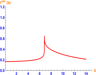
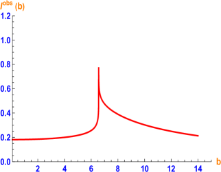
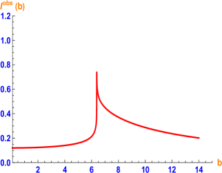
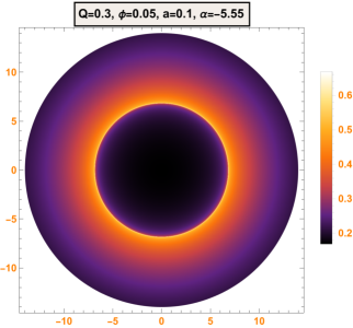
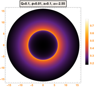
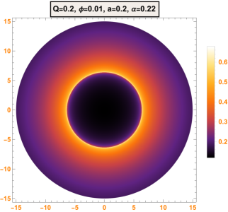
Figure 8: The graphical interpretation of the total observed intensity $I^{\text{obs}}(b)$, reflects by a static spherical accretion flow matter, for different BH state parameters and the mass of BH as $M=1$. We choose these numerical values as three examples, and one can find a comprehensive details in the main texts.

Based on Eq. (28), we will discuss the shadow appearance and related observed intensity of the considering BH in the perspective of static spherical accretion under the influence of parameters. The intensity of the light can be measured with the help of light pulse, which is calculated by the impact parameter $b$. In Fig. 8 (top row), the observed intensities of light rays are shown for various values of model parameters as mentioned in the two-dimensional BH shadow image in the bottom row.

From Fig. 1, we see that as the trajectory of impact parameter $b$ increases, the observed specific intensity starts to increase nicely and stay at the peak when $b=b_{c}$, and then exhibits a decaying pattern of attenuation. From Fig. 8 (top row), as $b$ increases, the intensity ascended first when $b<b_{c}$, then reached the peak value at $b=b_{c}$ and finally dropped down in the region $b>b_{c}$. This result is consistent with Fig. 1 and physically viable. When $b$ is smaller than the critical case $b_{c}$, the observed intensity originating from accretion matter is absorbed by the BH. For $b=b_{c}$, the trajectory of the photon is rotating about the BH several times in the BH photon ring orbit. Therefore, a distant static observer sees the maximal luminosity at the critical point.

Meanwhile, for $b>b_{c}$, the specific intensity $I^{\text{obs}}(b)$ shows a decaying behavior, and when $b\rightarrow\infty$, the observed intensity will be zero. Further, it is also observed that the intensity of the light ray gradually varies (increasing or decreasing) with the variation of parameters, and hence, each parameter plays a significant role in the BH luminosity. The two-dimensional BH shadow image is also reflected in Fig. 8 (bottom row), where different bright rings correspond to different values of the specific intensity. The image of the BH shadow is circularly symmetric, and BH is surrounded by a bright photon ring, so-called photon sphere. The numerical evaluation of photon sphere radius for some specific values of model parameters are listed in Table. 1. Clearly, the features in Fig. 8 are physically viable with that in Table. 1. Moreover, the interior of photon sphere does not vanish completely, because there is little part of radiative gas has escaped from the BH.

V Shadows of the BH with an Infalling Spherical Accretion

The geometrically thin accreting matter is assumed to be more realistic in nature due to infalling matters. Now Eq. (28) is still useful, but the associated red-shift factor defined as

$$g=\frac{\mathcal{K}_{\sigma}u_{0}^{\sigma}}{\mathcal{K}_{\tau}u_{e}^{\tau}},$$ (29)

in which $\mathcal{K}^{\rho}=\dot{x}_{\rho}$, $u_{0}^{\rho}=(1,0,0,0)$ and $u_{e}^{\rho}$ represent the four-velocity components of photon, static observer and accretion matter respectively, as given by

$$u_{e}^{s}=f(r)^{-1},\quad u_{e}^{v}=-(1-f(r))^{1/2},\quad u_{e}^{\theta}=u_{e}^{\varphi}=0.$$ (30)

Using Eqs. (12)-(14), we obtained the components of four-velocity. As $\mathcal{K}_{s}=1/b$ is a constant term and $\mathcal{K}_{v}$ can be inferred from $\mathcal{K}_{\varpi}\mathcal{K}^{\varpi}=0$, i.e.,

$$\frac{\mathcal{K}_{v}}{\mathcal{K}_{s}}=\pm\frac{1}{f(r)}\sqrt{1-\frac{b^{2}f(r)}{r^{2}}},$$ (31)

where the sign “$\pm$” corresponds to the motion of photons moving towards/away from the BH. Confronting Eq. (31), the red-shift factor given in Eq. (29) can be obtained as

$$g=\frac{1}{u_{e}^{s}+\mathcal{K}_{v}/\mathcal{K}_{e}u_{e}^{v}}.$$ (32)

In this case, the proper distance can be evaluated as

$$dl_{p}=\mathcal{K}_{\tau}u_{e}^{\tau}ds=\frac{\mathcal{K}_{s}}{g|\mathcal{K}_{v}|}dr,$$ (33)

where $\tau$ represents the photon path along the affine parameter $s$. Here, we also consider that the emissive specific intensity is monochromatic, so Eq. (26) is still valid and hence, the infalling spherical accretion can be calculated as

$$I^{\text{obs}}_{\star}(b)\propto\int g^{3}\mathcal{K}_{s}(r^{2}|\mathcal{K}_{v}|)^{-1}dr.$$ (34)

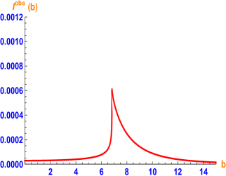
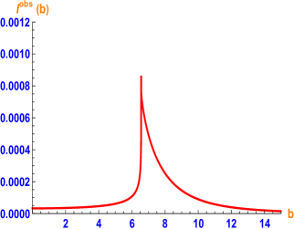
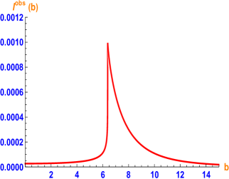
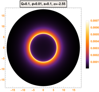
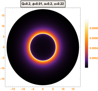
Figure 9: The graphical interpretation of the total observed intensity $I^{\text{obs}}_{\star}(b)$ reflects with an infalling spherical accretion flow matter, for different BH state parameters and the mass of BH as $M=1$. We choose these numerical values as three examples, and one can find a comprehensive details in the main texts.

From Eq. (34), we investigate the shadow of the considering BH by a static observer for different model parameters with infalling accretion. In Eq. (34), an absolute value of $\mathcal{K}_{v}$ is included, which represents that with the change of photon’s direction of motion, the sign of $\mathcal{K}_{v}$ also changed. From Fig. 9 (top row), we observed that the intensity of light increases significantly first as well to peak $b=b_{p}$, and then booster down to lower values. The observational features are relatively equivalent to that in the rest accretion case as we discussed earlier for Fig. 8.

The two-dimensional observational appearance of BH shadow image is shown in Fig. 9 (bottom row). We noticed that the resolution of the BH shadow and the location of the photon sphere are the similar phenomenological prescription as those with the static accretion flow. However, a major new disks viewed is found that in the central region, the infalling BH shadow has typically darker contribution in space-time properties as compared to that with static accretion, which is presumably accounted due to Doppler effect which relates the matter orbiting around the jet axis. More significantly, one can observe that the influence of this contribution is more prominent, which is close to the event horizon of the considering BH system.

VI Conclusions and Discussion

During the last two decades, the analysis of shadow cast by the astrophysical stellar objects, especially for BH and wormholes have been obtained significant attention in many research areas. The first detection of a BH shadow found at the hearts of giant galaxies from the EHT collaboration led to the more realistic interpretation of these astrophysical objects in nature. In the present study, we mainly investigate the shadows and photon spheres of BH, which is illuminated by a thin accretion disk. In this scenario, we have considered the optical appearance of four-dimensional Gauss-Bonnet BH in the presence of charge along with the cloud of strings and NC geometry of BH distribution.

For the viability of our developed structure in the framework of our considering BH shadow formulation, we have examined some physical properties under the influence of model parameters such as effective potential, deflection of light near the BH, shadows, and photon rings with optically and geometrically thin disk emission and observed specific intensities with static and infalling accretion flow models. The physical significance of the discussed properties for some specific choices of model parameters for our considered systems is listed below.

• Effective Potential: Using the effect of null geodesic, we depicted the behavior of effective potential and photon ring orbit in this geometry. From Fig. 1, one can see that the trajectories of effective potential significantly vary with the variations of parameters. Particularly, the value of the event horizon $r_{h}$, critical curve $b_{c}$ and photon sphere $r_{p}$ decreases with the increase of $\alpha$ and these quantities directly increase with increasing values of $a$. In addition, we also depicted the ingoing and outgoing trajectories of light rays corresponding to effective potential as shown in Figs. 2 and 3. For instant, we depicted here the behavior of effective potential just as example for some specific choices of model parameters and investigated the dynamics of the photon sphere under the influence of these values.

• Light Bending Near a BH: The optical appearance of accretion matter near the BH from a static observer’s eye can be understood by tracing the null geodesics. To understand the total change in the optical plane, we take three optical and geometrical accretion flow models as examples of null geodesic light trajectories with impact parameter $b$. We plotted this accretion in two different ways in Fig. 4. The top row of Fig. 4 shows the light ray trajectories according to the total number of orbits, $n(b)=\varphi/2\pi$. The motion of light rays in a straight line would correspond to $n(b)=1/2$, and the bending of light rays that do not enter the BH is calculated by $n(b)-1/2$. The singularity of these plots lie at $b=6.82781M$ (left panel), $b=6.55952M$ (Middle panel) and $b=6.38135M$ (right panel).

  The bottom row of Fig. 4 gives a clearer picture of what a static observer would see at large distances. The light rays can be classified into three regions such as direct emission, lensing ring and photon ring according to the number of distinctions at the equatorial plane. Despite these distinct configurations in the total luminosity of BH solutions, there is not only a dark interior the region, but also the direct emission makes a major contribution to the brightness while the lensing ring makes a minor contribution and the role of photon ring in observational appearance can be safely ignored regarding their negligible contribution.

• Transfer Functions: We try to understand the emission of light rays originating near the BH from an optically thin disk with the formulation of specific intensity depending on the radial coordinate. We plotted the first three transfer functions in Fig. 5. There is no light deflection inside the radius because none of the transfer functions has support for $b\leq 2.9M$. The slope of the first transfer function lies in the entire range, so the direct image represents the red-shift source file.

  The second transfer function supports the lensing ring and the image profile here is highly (de)magnified of the back side of the disk, while the third transfer function represents the photon ring, where the image is extremely demagnetized on the front side of the disk. This image profile as well as further images are highly demagnified, so, the contribution of these images is negligible to the total luminosity.

• Observational Features of BH: In addition, we considered three toy models of optically and geometrically thin disk emission flow to further study the observational appearance and then compared the observed specific intensities. The emitted intensity observed from these three models peaks at the isco for time-like observers, and at the unstable circular orbit for photons spheres and close the horizon for BH solution. The simulation obtained from specific intensities with the help of these three models yield different qualitative emissions and physical scenarios.

  From Figs. 6 and 7, the photon ring is an extremely curved light ray and has so narrow area and hence, the participation to the total flux can be negligible. The region of the lensing ring is wider than the photon ring and made a large contribution to the total flux. But this contribution is very small as compared to direct emission flow case. Hence, our obtained solutions showed that the role of direct emission is always appreciable to the total observed intensity.

• Specific Intensity with Static and Infalling Spherical Accretion: From the observed intensity, one can see that there is a bright sphere ring outside the central region and this brightness gradually varies with the influence of BH state parameters. In the case of infalling accretion, we found that the interior region of the shadow has lower observation luminosity than that of the static case, as one can see from the density map as depicted in Figs. 8 and 9. Furthermore, the static model has significantly lower trajectories than the infalling accretion one. So, the Doppler effect of infalling matter caused the most prominent contrast between these two accreting models. However, our considering BH parameters would change the position/location of the photon sphere BH profiles.

We obtained these results for a more realistic model as compared to 14 ; 15 and tried to enhance the brightness of the photon ring and BH shadow. We expect that these results inspire the theoretical study of BH shadow image and other physical quantities that may be fruitful for the observational teams working on achieving high resolution of the photon sphere and BH accreting matter configuration in GR as well as other modified theories of gravity.

References

- (1) B. Abbott et al, Observation of gravitational waves from a binary black hole merger, Phys. Rev. Lett. 116, 061102 (2016).
- (2) K. Akiyama et al., [Event Horizon Telescope Collaboration] First M87 event horizon telescope results. I. The shadow of the supermassive black hole. Astrophys. J. 875, L1 (2019).
- (3) K. Akiyama et al., [Event Horizon Telescope Collaboration, First M87 event horizon telescope results. II. Array and instrumentation. Astrophys. J. 875, L2 (2019).
- (4) K. Akiyama et al., [Event Horizon Telescope Collaboration], First M87 event horizon telescope results. III. Data processing and calibration. Astrophys. J. 875, L3 (2019).
- (5) K. Akiyama et al., [Event Horizon Telescope Collaboration], First M87 event horizon telescope results. IV. Imaging the central supermassive black hole. Astrophys. J. 875, L4 (2019).
- (6) K. Akiyama et al., [Event Horizon Telescope Collaboration], First M87 event horizon telescope results. V. Physical origin of the asymmetric ring. Astrophys. J. 875, L5 (2019).
- (7) K. Akiyama et al., [Event Horizon Telescope Collaboration], First M87 event horizon telescope results. VI. The shadow and mass of the central black hole. Astrophys. J. 875, L6 (2019).
- (8) R.M. Wald, General Relativity (The University of Chicago Press, 1984)
- (9) J.L. Synge, The escape of photons from gravitationally intense stars. Mon. Not. R. Astron. Soc. 131, 463 (1966). https://doi. org/10.1093/mnras/131.3.463
- (10) J.M. Bardeen, W.H. Press, S.A. Teukolsky, Rotating black holes: locally nonrotating frames, energy extraction, and scalar synchrotron radiation. Astrophys. J. 178, 347 (1972).
- (11) J.P. Luminet, Image of a spherical black hole with thin accretion disk. Astron. Astrophys. 75, 228 (1979).
- (12) S.E. Gralla, D.E. Holz, R.M. Wald, Black Hole shadows, photon rings, and lensing rings. Phys. Rev. D 100, 024018 (2019).
- (13) H. Falcke, F. Melia, E. Agol, Viewing the shadow of the black hole at the galactic center. Astrophys. J. 528, L13 (2000).
- (14) X.X. Zeng, H.Q. Zhang, Influence of quintessence dark energy on the shadow of black hole. Eur. Phys. J. C 80, 1058 (2020).
- (15) X.X. Zeng, H.Q. Zhang, H. Zhang, Shadows and photon spheres with spherical accretions in the four-dimensional Gauss-Bonnet black hole. Eur. Phys. J. C 80, 872 (2020).
- (16) Ma, Liang, H. Lü, Bounds on photon spheres and shadows of charged black holes in Einstein-Gauss-Bonnet-Maxwell gravity, Phys. Lett. B 807, 135535 (2020).
- (17) Y. X. Gao, Y. Xie, Gravitational lensing by hairy black holes in Einstein-scalar-Gauss-Bonnet theories, Phys. Rev. D. 103, 043008 (2021).
- (18) S. Guo, K. J. He, G. R. Li, G. P. Li, The shadow and photon sphere of the charged black hole in Rastall gravity, Class. Quant. Grav. 38, 165013 (2021).
- (19) S. Guo, G. R. Li, E. W. Liang, Influence of accretion flow and magnetic charge on the observed shadows and rings of the Hayward black hole, Phys. Rev. D. 105, 023024 (2022).
- (20) R. Shaikh, P. Kocherlakota, R. Narayan, P.S. Joshi, Shadows of spherically symmetric black holes and naked singularities. Mon. Not. Roy. Astron. Soc. 482, 52 (2019).
- (21) S. Vagnozzi, L. Visinelli, Hunting for extra dimensions in the shadow of . Phys. Rev. D 100, 024020 (2019).
- (22) R.A. Konoplya, A.F. Zinhailo, Quasinormal modes, stability and shadows of a black hole in the novel 4D Einstein-Gauss-Bonnet gravity. Eur. Phys. J. C 80, 1 (2020).
- (23) R.A. Konoplya, Shadow of a black hole surrounded by dark matter. Phys. Lett. B 795, 1 (2019).
- (24) M. Zhang, M. Guo, Can shadows reflect phase structures of black holes? Eur. Phys. J. C 80, 1 (2020).
- (25) Saurabh, K. Jusufi, Imprints of dark matter on black hole shadows using spherical accretions. Eur. Phys. J. C 81, 1 (2021).
- (26) K.J. He, S.C, Tan, G.P, Li, Influence of torsion charge on shadow and observation signature of black hole surrounded by various profiles of accretions. Eur. Phys. J. C 82, 1 (2022).
- (27) X.X. Zeng, G.P. Li, K.J. He, The shadows and observational appearance of a noncommutative black hole surrounded by various profiles of accretions. Nuc. Phys. B 974, 115639 (2022).
- (28) P. Nicolini, Noncommutative black holes, the final appeal to quantum gravity: a review. Int. J. Mod. Phys. A 24, 1229 (2009).
- (29) H.S. Snyder, Quantized space-time. Phys. Rev. 71 38 (1947).
- (30) G.P. Li, K.J. He, B.B. Chen, Lorentz violation, quantum tunneling and information conservation. Chi. Phys. C 45, 015111 (2021).
- (31) P. Aschieri, C. Blohmann, M. Dimitrijevic, F. Meyer, P. Schupp, J. Wess, A gravity theory on noncommutative spaces. Clas. Quant. Grav. 22, 3511 (2005).
- (32) P. Aschieri, M. Dimitrijevic, F. Meyer, J. Wess, Noncommutative geometry and gravity. Class. Quantum Gravity 23, 1883 (2006).
- (33) D.V. Singh, S.G. Ghosh, S.D. Maharaj (2020). Clouds of strings in Einstein-Gauss-Bonnet black holes. Phys. Dark. Uni, 30, 100730 (2020).
- (34) M.A. Anacleto, F.A. Brito, J.A.V. Campos, E. Passos. Absorption and scattering of a noncommutative black hole. Phys. Lett. B 803, 135334 (2020).
- (35) D. Glavan, C. Lin, Einstein-Gauss-Bonnet Gravity in Four-Dimensional Spacetime. Phys. Rev. Lett. 124, 081301 (2020).
- (36) S.E. Gralla, A. Lupsasca, Lensing by Kerr black holes. Phys. Rev. D 101, 044031 (2020).
- (37) D.N. Page, K.S. Thorne, Disk-accretion onto a black hole. Astrophys. J. 191, 499 (1974).
- (38) M. Guerrero, G.J. Olmo, D. Rubiera-Garcia, D.S.C. Gómez, Shadows and optical appearance of black bounces illuminated by a thin accretion disk. JCAP. 08, 036 (2021).
- (39) M. Jaroszynski, A. Kurpiewski, Optics near Kerr black holes. spectra of advection dominated accretion flows. Astron. Astrophys. 326, 419 (1997).
- (40) C. Bambi, Can the supermassive objects at the centers of galaxies be traversable wormholes? The first test of strong gravity for mm/submm very long baseline interferometry facilities. Phys. Rev. D 87, 107501 (2013).