A new approach to color-coherent parton evolution

Abstract

We present a simple parton-shower model that replaces the explicit angular ordering of the coherent branching formalism with a differentially accurate simulation of soft-gluon radiation by means of a non-trivial dependence of the splitting functions on azimuthal angles. We introduce a global kinematics mapping and provide an analytic proof that it satisfies the criteria for next-to leading logarithmic accuracy. In the new algorithm, initial and final state evolution are treated on the same footing. We provide an implementation for final-state evolution in the numerical code Alaric and present a first comparison to experimental data.

I Introduction

Parton showers are a cornerstone of computer simulations for high-energy collider physics Buckley et al. (2011); Campbell et al. (2022). They implement the evolution of QCD from the hard scales to be probed by experiments, to the low scale of hadronization, where the transition of quasi-free partons (the quarks and gluons of perturbative QCD) to observable hadrons occurs. In this process, a number of additional partons are generated according to evolution equations that are based on the factorization properties of QCD amplitudes in the soft and collinear limits. The most commonly used parton showers can be thought of as numerical implementations of the DGLAP equations Dokshitzer (1977); Gribov and Lipatov (1972); Lipatov (1975); Altarelli and Parisi (1977), but various other approaches exist Lönnblad (1992); Kharraziha and Lönnblad (1998); Jung and Salam (2001).

The first generation of parton shower programs Webber (1984); Bengtsson et al. (1986); Bengtsson and Sjöstrand (1987a); Marchesini and Webber (1988); Andersson et al. (1990) was developed four decades ago. Implementations differed in the way in which the ordering inherent to the evolution equations was realized in the simulation, and how the kinematics of the emissions were set up. Color coherence, manifesting itself through angular ordering Mueller (1981); Ermolaev and Fadin (1981); Dokshitzer et al. (1982a, b, 1983); Bassetto et al. (1982) became a guiding principle for the construction of parton showers Webber (1986); Bengtsson and Sjöstrand (1987b). Some of these parton showers were also improved using spin correlation algorithms Collins (1988); Knowles (1988a, b, 1990). Increasing precision requirements, especially in preparation for the Large Hadron Collider (LHC), mandated more precise Monte-Carlo simulations. The matching of parton showers to next-to-leading order calculations Frixione and Webber (2002); Nason (2004); Frixione et al. (2007); Alioli et al. (2010); Höche et al. (2011, 2012); Alwall et al. (2014) and the merging of calculations for varying jet multiplicity Catani et al. (2001); Lönnblad (2002); Krauss (2002); Alwall et al. (2008); Höche et al. (2009); Lönnblad and Prestel (2012); Gehrmann et al. (2013); Höche et al. (2013); Frederix and Frixione (2012); Lönnblad and Prestel (2013); Plätzer (2013) became focus points of event generator development. The correspondence between fixed-order infrared subtraction schemes and parton showers was identified as central to a correct matching procedure, leading to the construction of algorithms with a dipole-local momentum mapping and ordering in transverse momentum Nagy and Soper (2005, 2006); Schumann and Krauss (2008); Giele et al. (2008); Plätzer and Gieseke (2011); Höche and Prestel (2015); Fischer et al. (2016); Cabouat and Sjöstrand (2018).

These newly developed algorithms were found to have significant drawbacks in terms of their logarithmic accuracy Dasgupta et al. (2018). The resummation of observables at leading logarithmic (LL) accuracy is relatively straightforward to achieve using a parton-shower algorithm. The resummation at next-to-leading logarithmic (NLL) precision however poses a number of challenges. The first generic technique to quantify the logarithmic accuracy of parton showers was presented in Dasgupta et al. (2018, 2020) and consists of a set of fixed-order and all-order criteria, which can broadly be classified as tests related to kinematic recoil effects, and tests of color coherence. In the present manuscript, we will discuss only kinematic effects. A discussion of sub-leading color effects can be found for example in Nagy and Soper (2012); Plätzer and Sjödahl (2012); Nagy and Soper (2014, 2015); Plätzer et al. (2018); Isaacson and Prestel (2019); Nagy and Soper (2019a, b); Forshaw et al. (2019); Höche and Reichelt (2021); De Angelis et al. (2021); Holguin et al. (2021); Hamilton et al. (2021). One of the main results of Dasgupta et al. (2018) was that the kinematics mapping in the transition from an $n$-particle to an $n+1$-particle final state should not alter the existing momentum configuration in a way that distorts the effects of the pre-existing emissions on observables. This criterion is formulated such that only the effects relevant at NLL precision can be extracted, by taking the limit $\alpha_{s}\to 0$ at fixed $\lambda=\alpha_{s}\ln v$, where $v$ is the observable to be resummed. The algorithms in Schumann and Krauss (2008); Höche and Prestel (2015); Cabouat and Sjöstrand (2018) do not satisfy the criteria for NLL precision, because their momentum mappings can generate recoil whose effect on existing emissions at commensurate scales does not vanish in the $\alpha_{s}\to 0$ limit. It is important to note that these failures to agree with known NLL resummation are not related to the effects of momentum and probability conservation discussed in Höche et al. (2018). In order to remedy the problem with NLL accuracy, new kinematics mapping schemes were developed in Bewick et al. (2020); Forshaw et al. (2020); Dasgupta et al. (2020); van Beekveld et al. (2022). The main difference of the new dipole schemes in Dasgupta et al. (2020); van Beekveld et al. (2022) compared to existing algorithms is that recoil is assigned according to the rapidity of the emission in the frame of the hard process, rather than the dipole frame, and that initial-state radiation is treated such that the interpretation of the hard system is unchanged for subsequent emissions.

We will approach the same problem from a different perspective. Recalling that color–coherent parton evolution is a consequence of the angular dependence of the soft eikonal, we will reformulate the radiator functions of Webber (1986) using a partial fractioning approach similar to the identified particle subtraction scheme in Catani and Seymour (1997). In addition, we note that in dipole and antenna showers the anti-collinear direction is inextricably linked to the direction of the color spectator. By lifting this restriction, we are able to construct an algorithm which allows the entire QCD multipole to absorb the recoil from parton branching, independent of the number of pre-existing emissions, and independent of their kinematics. The price for such a generic scheme is a dependence of the parton shower splitting functions on the azimuthal angle between the decay plane and the plane defined by the emitting parton and its color spectator. Our new formulation presents a major extension of existing parton shower formalisms in this regard, and it introduces the most generic form of a spin-averaged splitting function in four dimensions, with a dependence on all three phase-space variables of the radiated parton. Based on previous analyses Höche and Prestel (2017); Dulat et al. (2018), it seems plausible that this scheme will considerably simplify the inclusion of higher-order corrections to the splitting kernels. We provide a first implementation of the new algorithm in the numerical code Alaric , which will be made available as part of the event generator Sherpa Gleisberg et al. (2004, 2009); Bothmann et al. (2019).

This manuscript is organized as follows: In Sec. II we revisit the soft singularity structure of QCD amplitudes and introduce our new decomposition of the soft eikonal. In Sec. III we discuss the novel phase-space mapping and the corresponding phase-space factorization. In Sec. IV we detail how soft and collinear emissions are generated in a probabilistic picture. Section V is dedicated to the analytic proof of logarithmic accuracy, and the numerical validation in the $\alpha_{s}\to 0$ limit. Section VI presents first numerical results for the process $e^{+}e^{-}\to\,$hadrons, and Sec. VII contains an outlook.

II The matching of soft to collinear radiators

We start the discussion by recalling the singularity structure of $n$-parton QCD amplitudes in the infrared limits.

If two partons, $i$ and $j$, become collinear, the squared amplitude factorizes as

$${}_{n}\langle 1,\ldots,n|1,\ldots,n\rangle_{n}=\sum_{\lambda,\lambda^{\prime}=\pm}\,{}_{n-1}\Big{<}1,\ldots,i\!\!\backslash(ij),\ldots,j\!\!\!\backslash,\ldots,n\Big{|}\frac{8\pi\alpha_{s}}{2p_{i}p_{j}}P^{\lambda\lambda^{\prime}}_{(ij)i}(z)\Big{|}1,\ldots,i\!\!\backslash(ij),\ldots,j\!\!\!\backslash,\ldots,n\Big{>}_{n-1}\;,$$ (1)

where the notation $i\!\!\backslash$ indicates that parton $i$ is removed from the original amplitude, and where $(ij)$ is the progenitor of partons $i$ and $j$. The functions $P^{\lambda\lambda^{\prime}}_{ab}(z)$ are the spin-dependent DGLAP splitting functions. They depend on the momentum fraction $z$ of parton $i$ with respect to the mother parton, $(ij)$, and on the helicities $\lambda$ Dokshitzer (1977); Gribov and Lipatov (1972); Lipatov (1975); Altarelli and Parisi (1977). In the collinear limit, the momentum fraction is equal to an energy or light-cone momentum fraction. In this manuscript we will consider only spin-averaged splitting functions; algorithms for spin-dependent evolution are discussed in Collins (1988); Knowles (1988a, b, 1990); Hamilton et al. (2022).

In the limit that gluon $j$ becomes soft, the squared amplitude factorizes as Bassetto et al. (1983)

$${}_{n}\langle 1,\ldots,n|1,\ldots,n\rangle_{n}=-8\pi\alpha_{s}\sum_{i,k\neq j}\,{}_{n-1}\big{<}1,\ldots,j\!\!\!\backslash,\ldots,n\big{|}{\bf T}_{i}{\bf T}_{k}\,w_{ik,j}\big{|}1,\ldots,j\!\!\!\backslash,\ldots,n\big{>}_{n-1}\;,$$ (2)

where ${\bf T}_{i}$ and ${\bf T}_{k}$ are the color insertion operators defined in Catani and Seymour (1997). In the remainder of this section we will discuss the case of massless radiators only and focus on the eikonal factor, $w_{ik,j}$, and how it can be rewritten in a suitable form to match the spin-averaged splitting functions $P_{ab}(z)$ in the soft-collinear limit. Since our analysis concerns only the denominator of $w_{ik,j}$, it will apply to spin-correlated evolution as well. The eikonal factor is given by

$$w_{ik,j}=\frac{p_{i}p_{k}}{(p_{i}p_{j})(p_{j}p_{k})}\;,$$ (3)

and it can be written in terms of (frame-dependent) energies and angles as

$$w_{ik,j}=\frac{W_{ik,j}}{E_{j}^{2}}\;,\qquad\text{where}\qquad W_{ik,j}=\frac{1-\cos\theta_{ik}}{(1-\cos\theta_{ij})(1-\cos\theta_{jk})}\;,$$ (4)

We note that Eq. (4) is symmetric in $i$ and $k$, and that it encapsulates the complete soft singularity structure of the hard matrix element Bassetto et al. (1983). If we were to implement Eq. (4) for each of the radiators $i$ and $k$ in the collinear limit, we would therefore double-count the most singular component of the emission probability Ellis et al. (1996). This is known as the soft double-counting problem, which can be solved by following the technique of Webber (1986). In this approach, $W_{ik,j}$ is written as a sum of two terms, which are enhanced only in either the $ij$- or $kj$-collinear limit:

$$W_{ik,j}=\tilde{W}_{ik,j}^{i}+\tilde{W}_{ki,j}^{k}\;,\qquad\text{where}\qquad\tilde{W}_{ik,j}^{i}=\frac{1}{2}\left(\frac{1-\cos\theta_{ik}}{(1-\cos\theta_{ij})(1-\cos\theta_{jk})}+\frac{1}{1-\cos\theta_{ij}}-\frac{1}{1-\cos\theta_{jk}}\right)\;.$$ (5)

It is customary to define the $z$-axis to be aligned with the momentum $p_{i}$, such that we can write $\cos\theta_{jk}$ in terms of polar angles, $\theta_{j}^{\,i}$, $\theta_{k}^{\,i}$ with respect to the axis defined by $p_{i}$, and the azimuthal angle $\phi_{jk}^{\,i}$ in the same frame. Note in particular that $\theta_{l}^{\,i}=\theta_{li}$, for any $l$.

$$\cos\theta_{jk}=\cos\theta_{j}^{\,i}\cos\theta_{k}^{\,i}+\sin\theta_{j}^{\,i}\sin\theta_{k}^{\,i}\cos\phi_{jk}^{\,i}\;.$$ (6)

When performing the azimuthal averaging, we find the simple result Webber (1986)

$$\frac{1}{2\pi}\int_{0}^{2\pi}{\rm d}\phi_{jk}^{i}\tilde{W}_{ik,j}^{i}=\frac{\tilde{I}_{ik,j}^{i}}{1-\cos\theta_{j}^{\,i}}\;,\qquad\text{where}\qquad\tilde{I}_{ik,j}^{i}=\left\{\begin{array}[]{cc}1&\quad\text{if}\quad\theta_{j}^{\,i}<\theta_{k}^{\,i}\\[5.69054pt] 0&\quad\text{else}\end{array}\right.\;.$$ (7)

The behavior of $\tilde{I}_{ik,j}^{i}$ as a function of the polar angles is known as angular ordering, which means that the total probability for soft radiation averages to zero outside of a cone defined by the cusp angle $\theta_{k}^{\,i}$ of the radiating color dipole. This is the origin of the coherent branching formalism and the basis for angular ordered parton showers. It is instructive to investigate this radiation pattern in more detail.

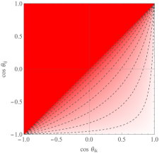
(a)

(b)

(c)

Figure 1: Azimuthally integrated radiator functions. Figures 1(a) and 1(b) show the positive and negative contributions to $\tilde{I}_{ik,j}^{i}$ arising from the additive matching in Eq. (5), Fig. 1(c) displays $\bar{I}_{ik,j}^{i}$ from the multiplicative matching in Eq. (9).

Figures 1(a) and 1(b) display the positive and negative contribution to the azimuthal integral, normalized to $2\pi$, as a function of the polar angles. The partial radiator function $\tilde{W}_{ik,j}^{i}$ has a root at

$$\cos\phi_{jk}^{\,i(0)}=-\sqrt{\frac{1+\cos\theta_{j}^{\,i}}{1-\cos\theta_{j}^{\,i}}\,\frac{1-\cos\theta_{k}^{\,i}}{1+\cos\theta_{k}^{\,i}}}$$ (8)

which falls inside the integration domain if $\theta_{j}^{\,i}>\theta_{k}^{\,i}$. In this case, the negative contribution to the azimuthal integral is equal in magnitude to the positive contribution, such that the average radiation probability vanishes identically. However, there is a strong modulation of this probability as a function of the azimuthal angle. If this modulation is not included in a parton-shower simulation, wide-angle soft radiation effects will only be captured correctly for observables that are sufficiently insensitive to the precise distribution of radiation in phase space.

A naive attempt to solving this problem would be to include the full azimuthal dependence of the radiator function in the Monte-Carlo simulation. Such an approach is bound to fail, because in the region $\theta_{j}^{\,i}>\theta_{k}^{\,i}$ one would need to sample the same amount of negative and positive weighted Monte-Carlo events, leading to an efficiency of exactly zero. We therefore adopt a different strategy, pioneered in Catani and Seymour (1997), where the radiator function is partial fractioned such that it maintains strict positivity

$$W_{ik,j}=\bar{W}_{ik,j}^{i}+\bar{W}_{ki,j}^{k}\;,\qquad\text{where}\qquad\bar{W}_{ik,j}^{i}=\frac{1-\cos\theta_{ik}}{(1-\cos\theta_{ij})(2-\cos\theta_{ij}-\cos\theta_{jk})}\;.$$ (9)

Azimuthal averaging again leads to Eq. (7), except that $\tilde{I}_{ik,j}^{i}$ is replaced by

$$\bar{I}_{ik,j}^{i}=\frac{1}{\sqrt{(\bar{A}_{ij,k}^{\,i})^{2}-(\bar{B}_{ij,k}^{\,i})^{2}}}\;,$$ (10)

where

$$\bar{A}_{ij,k}^{\,i}=\frac{2-\cos\theta_{j}^{\,i}(1+\cos\theta_{k}^{\,i})}{1-\cos\theta_{k}^{\,i}}\;\qquad\text{and}\qquad\bar{B}_{ij,k}^{\,i}=\frac{\sqrt{(1-\cos^{2}\theta_{j}^{\,i})(1-\cos^{2}\theta_{k}^{\,i})}}{1-\cos\theta_{k}^{\,i}}\;.$$ (11)

This function is shown in Fig. 1(c). As required, it approaches unity in the limit $\theta_{j}^{\,i}\to 0$, independent of the value of $\theta_{k}^{\,i}$, and also for the special case of a back-to-back configuration, $\theta_{k}^{\,i}\to\pi$. While the Monte-Carlo efficiency of an algorithm using this technology will be reduced compared to plain angular ordered evolution, the obvious benefit is that Eq. (9) allows to capture all angular correlations associated with the spin-summed soft eikonal, Eq. (4). In contrast, traditional angular ordered evolution, which is based on Eq. (7), does not populate the complete emission phase space, necessitating intricate matrix-element corrections and creating complications in higher-order matching Frixione and Webber (2002). We note again that the energy $E_{j}$ in Eq. (4) is frame dependent. This effect will be discussed in more detail in Sec. IV.1.

In the limit where partons $i$ and $j$ are collinear, we can write the eikonal factor in Eq. (3) as

$$w_{ik,j}\overset{i||j}{\longrightarrow}w_{ik,j}^{\rm(coll)}(z)=\frac{1}{2p_{i}p_{j}}\frac{2z}{1-z}\;,\qquad\text{where}\qquad z\overset{i||j}{\longrightarrow}\frac{E_{i}}{E_{i}+E_{j}}\;.$$ (12)

This can be identified with the leading term (in $1-z$) of the DGLAP splitting functions $P_{aa}(z)$, where 

$$\begin{split}P_{qq}(z)&=C_{F}\left(\frac{2z}{1-z}+(1-z)\right)\;,\\ P_{gg}(z)&=C_{A}\left(\frac{2z}{1-z}+z(1-z)\right)\;,\\ P_{gq}(z)&=T_{R}\left(1-2z(1-z)\right)\;.\end{split}$$ (13)

To match the soft to the collinear splitting functions, we therefore replace

$$\frac{1}{2p_{i}p_{j}}P_{(ij)i}(z)\to\frac{1}{2p_{i}p_{j}}P_{(ij)i}(z)+\delta_{(ij)i}\,{\bf T}_{i}^{2}\Bigg{[}\frac{\bar{W}_{ik,j}^{i}}{E_{j}^{2}}-w_{ik,j}^{\rm(coll)}(z)\Bigg{]}\;,$$ (14)

where the two contributions to the gluon splitting function are treated as two different radiators Höche and Prestel (2015). This substitution introduces a dependence on a color spectator, $k$, whose momentum defines a direction independent of the direction of the collinear splitting. In general, this implies that splitting functions which were formerly dependent only on a momentum fraction along this direction, now acquire a dependence on the remaining two phase-space variables of the new parton. This is the most general form of a splitting kernel for spin-averaged parton evolution, which we will use in the following. In particular, the dependence on the azimuthal angle allows to define the recoil momentum such that NLL precision is maintained for any hard process, as discussed in more detail in Sec. V.

III Momentum mapping and phase-space factorization

The mapping of Born momenta to a kinematic configuration after emission of additional partons is a key component of any parton shower algorithm. It is closely tied to the factorization of the Lorentz-invariant differential phase space element for a multi-parton configuration. Suitable momentum mappings will preserve the key features of previously simulated radiation, while an unsuitable mapping could skew the QCD radiation pattern up to a point where it becomes not only theoretically incorrect, but the differences become visible experimentally. A prime, although academic, example for the latter problem is a collinear unsafe mapping algorithm, in which the parton shower does not reflect the features of the collinear limit of the QCD matrix elements, Eq. (3) and therefore introduces an error at leading logarithmic accuracy. A key requirement for the construction of any momentum mapping therefore is collinear safety, and all known parton-shower algorithms satisfy this constraint. An example for a problem which may only be seen in dedicated measurements was identified in Dasgupta et al. (2018). It originates in a modification of existing soft momenta in subsequent emissions, that introduces an error in the simulated QCD radiation pattern at next-to-leading logarithmic accuracy. In the following, we will construct a generic, collinear and NLL safe momentum mapping for both final-state and initial-state radiation, which is inspired by the identified–particle dipole subtraction algorithm in Catani and Seymour (1997). We will provide the analytic proof of NLL safety in Sec. V.1 and sketch the additional steps that are required to match the parton shower to NLO calculations in Appendix C.

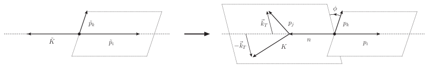
Figure 2: Sketch of the momentum mapping for final-state evolution. See the main text for details. Note that $p_{k}$ does not participate in the shift, Eq. (17), and only acts as a reference for the azimuthal angle $\phi$.

We begin by describing the logic underpinning our new kinematics mapping, $\{\tilde{p}_{l}\}\to\{p_{l}\}$. We identify the splitter momentum, $\tilde{p}_{i}$, and define a recoil momentum, $\tilde{K}$, as the negative sum of all momenta in the radiating QCD multipole, including the momentum of the splitter (see also Appendix A). Together, the momenta $\tilde{K}$ and $\tilde{p}_{i}$ define the reference frame of the splitting, as shown schematically in Fig. 2 (left). The momentum of the color spectator, $\tilde{p}_{k}$, defines an additional direction, which provides the reference for the azimuthal angle, $\phi$. In the first step of the mapping, the emitter momentum is scaled by a factor $z$, and the emitted momentum, $p_{j}$, is constructed with transverse momentum component $\vec{k}_{T}$ and suitable light-cone momenta. The color spectator remains unchanged, $p_{k}=\tilde{p}_{k}$. The recoil is absorbed by the overall multipole, such that after the emission we have $K\neq\tilde{K}$, while $K^{2}=\tilde{K}^{2}$. In particular, the multipole after the emission acquires a transverse momentum with respect to $\tilde{K}$. This is shown schematically in Fig. 2 (right). To compensate for both the transverse and the longitudinal recoil, the overall multipole is boosted to its original frame of reference. This changes all momenta and effectively distributes the recoil among them, generating changes of the order of ${\rm k}_{T}/\sqrt{K^{2}}$, which vanish in the infrared limits. We will make use of this fact in Sec. V.1.

A collinear safe momentum mapping requires that for any two massless collinear partons, $i$ and $j$, the momenta behave as

$$p_{i}\overset{i||j}{\longrightarrow}z\,\tilde{p}_{i}\;,\qquad p_{j}\overset{i||j}{\longrightarrow}(1-z)\,\tilde{p}_{i}\;.$$ (15)

In the exact limit, $\cos\theta_{ij}=0$, the splitting variable $z$ is uniquely defined and given by

$$z=\frac{p_{i}n}{(p_{i}+p_{j})n}\;.$$ (16)

where $n$ is an arbitrary auxiliary vector that satisfies $\tilde{p}_{i}n\neq 0$. Note that $n$ can be either light-like, time-like or space-like, as long as $\tilde{p}_{i}n\neq 0$. In order to construct a collinear-safe momentum mapping for arbitrary values of the two-particle virtuality $p_{i}p_{j}$, we can simply use the first part of Eq. (15) away from this limit. This implies in particular that $p_{i}$ retains its direction, and that all angular radiator functions involving $p_{i}$ remain unchanged.

A second important constraint for the mapping is overall four-momentum conservation. We satisfy this by defining a vector $\tilde{K}$ to be a combination of the momenta $\{\tilde{p}_{1},\ldots,\tilde{p}_{j-1},\tilde{p}_{j+1},\ldots,\tilde{p}_{n}\}$, and by using the shift

$$p_{i}=z\,\tilde{p}_{i}\;,\qquad n=\tilde{K}+(1-z)\,\tilde{p}_{i}\;,$$ (17)

which implies $p_{i}+n=\tilde{p}_{i}+\tilde{K}$. The remaining task is to construct two new vectors, $K$ and $p_{j}$, such that $K^{2}=\tilde{K}^{2}$, and such that $p_{j}$ satisfies the collinear safety constraint, Eq. (15). The momenta in $\tilde{K}$ are mapped to new momenta by a Lorentz transformation that is defined in terms of $\tilde{K}$ and $K$. The simplest way to obtain the new momenta is by means of a light-cone parametrization Sudakov (1956). With the help of the light-like vector

$$\bar{n}=n-\frac{n^{2}}{2\tilde{p}_{i}n}\,\tilde{p}_{i}=\tilde{K}-\kappa\,\tilde{p}_{i}\;,\qquad\text{where}\qquad\kappa=\frac{\tilde{K}^{2}}{2\tilde{p}_{i}\tilde{K}}\;.$$ (18)

we can write

$$\begin{split}p_{j}&=v\,\bar{n}+\frac{1}{v}\frac{{\rm k}_{\perp}^{2}}{2\tilde{p}_{i}\tilde{K}}\,\tilde{p}_{i}-k_{\perp}\;,&\text{where}\qquad v&=\frac{p_{i}p_{j}}{p_{i}\tilde{K}}\\ K&=(1-v)\,\bar{n}+\frac{1}{1-v}\frac{{\rm k}_{\perp}^{2}+\tilde{K}^{2}}{\,2\tilde{p}_{i}\tilde{K}}\,\tilde{p}_{i}+k_{\perp}\;.\end{split}$$ (19)

Equation (19) makes it manifest that $\tilde{K}$ absorbs the newly generated transverse and anti-collinear momentum when parton $(ij)$ is put off-shell, such that overall momentum conservation is satisfied. This leads to the identity

$${\rm k}_{\perp}^{2}=v(1-v)\,2p_{j}K-v^{2}K^{2}=v(1-v)(1-z)\,2\tilde{p}_{i}\tilde{K}-v^{2}\tilde{K}^{2}\;.$$ (20)

Note that ${\rm k}_{\perp}^{2}$ is proportional to $v$ and therefore tends to zero in the collinear limit $\cos\theta_{j}^{\,i}\to 0$. Inserting this relation into Eq. (19) makes both collinear safety and overall four-momentum conservation of the kinematics mapping manifest.

$$\begin{split}p_{j}&=(1-z)\,\tilde{p}_{i}+v\big{(}\tilde{K}-(1-z+2\kappa)\,\tilde{p}_{i}\big{)}+k_{\perp}\;,\\ K&=\hskip 31.29802pt\tilde{K}-v\big{(}\tilde{K}-(1-z+2\kappa)\,\tilde{p}_{i}\big{)}-k_{\perp}\;.\end{split}$$ (21)

In order to determine a reference direction for the azimuthal angle $\phi=\arctan({\rm k}_{y}/{\rm k}_{x})$, we note that the soft radiation pattern of Eq. (9) must be correctly generated. To achieve this we decompose the transverse momentum as

$$k_{\perp}^{\mu}={\rm k}_{\perp}\left(\cos\phi\,\frac{n_{\perp}^{\mu}}{|n_{\perp}|}+\sin\phi\,\frac{l_{\perp}^{\,\mu}}{|l_{\perp}|}\right)\;,$$ (22)

where the reference axes $n_{\perp}$ and $l_{\perp}$ are given by the transverse projections

$$n_{\perp}^{\mu}=p_{k}^{\mu}-\frac{p_{k}\bar{n}}{\tilde{p}_{i}\tilde{K}}\,\tilde{p}_{i}^{\mu}-\frac{p_{k}\tilde{p}_{i}}{\tilde{p}_{i}\tilde{K}}\,\bar{n}^{\mu}\;,\qquad\text{and}\qquad l_{\perp}^{\,\mu}=\varepsilon^{\mu}_{\;\nu\rho\sigma}\,\tilde{p}_{i}^{\,\nu}\,\bar{n}^{\,\rho}\,n_{\perp}^{\sigma}\;.$$ (23)

Because the differential emission phase-space element, Eq. (28), is a Lorentz-invariant quantity, the azimuthal angle $\phi$ is Lorentz invariant. It can be expressed as

$$\phi=\arccos\frac{(p_{i}p_{j})(p_{k}{\bar{n}})+(p_{i}p_{k})(p_{j}{\bar{n}})-(p_{i}{\bar{n}})(p_{j}p_{k})}{\sqrt{2(p_{i}p_{j})(p_{j}{\bar{n}})}\sqrt{2(p_{i}p_{k})(p_{k}{\bar{n}})}}\;.$$ (24)

This allows us to write the emission phase space in a frame-independent way. After the momenta $p_{i}$, $p_{j}$ and $K$ are constructed, the momenta $\{p_{l}\}$ used to define $\tilde{K}$ are subjected to a Lorentz transformation, which can be written as Catani and Seymour (1997)

$$p_{l}^{\mu}\to\Lambda^{\mu}_{\;\nu}(\tilde{K},K)\,p_{l}^{\nu}\;,\qquad\text{where}\qquad\Lambda^{\mu}_{\;\nu}(\tilde{K},K)=g^{\mu}_{\;\nu}-\frac{2(K+\tilde{K})^{\mu}(K+\tilde{K})_{\nu}}{(K+\tilde{K})^{2}}+\frac{2K^{\mu}\tilde{K}_{\nu}}{\tilde{K}^{2}}\;.$$ (25)

If needed, the event is restored to the lab frame, as described in App. A. We list the precise algorithm for the construction of final-state splittings in Sec. A.1, and give the algorithm for the construction of initial-state splittings in Sec. A.2. The initial-state kinematics are obtained by the simple replacement $z\to x=1/z$, as indicated by crossing relations.

The last remaining task is to determine the differential emission phase space element. We will outline how to do this for pure final-state evolution, where the recoil partner $\tilde{K}$ corresponds to the sum of the initial state momenta. This covers the important case of the decay of a color-neutral, massive particle, such as a $Z$-boson at LEP. Since $K$, $\tilde{K}$ and $n$ are treated as outgoing, they appear with negative energy component, which requires the explicit compensation of a number of minus signs that do not appear in the case where $\tilde{K}$ corresponds to a part of the final state. The general discussion can be found in App. B.

The differential phase-space element for $(n-1)$ hard momenta, $\{p_{1},\ldots,p_{j-1},p_{j+1},\ldots,p_{n}\}$, and one soft momentum, $p_{j}$, is defined as

$$\begin{split}{\rm d}\Phi_{n}(p_{a},p_{b};p_{1},\ldots,p_{n})=&\;\left[\prod_{i=1}^{n}\frac{1}{(2\pi)^{3}}\frac{{\rm d}^{3}p_{i}}{2p_{i}^{0}}\right](2\pi)^{4}\delta^{(4)}(p_{a}+p_{b}-\sum p_{i})\;.\end{split}$$ (26)

It can be written in terms of the differential phase-space element for the momenta $\{\tilde{p}_{1},\ldots,\tilde{p}_{j-1},\tilde{p}_{j+1},\ldots,\tilde{p}_{n}\}$ before the mapping

$$\begin{split}{\rm d}\Phi_{n-1}(\tilde{p}_{a},\tilde{p}_{b};\tilde{p}_{1},\ldots,\tilde{p}_{j-1},\tilde{p}_{j+1},\ldots,\tilde{p}_{n})=&\;\Bigg{[}\prod_{\begin{subarray}{c}i=1\\ i\neq j\end{subarray}}^{n}\frac{1}{(2\pi)^{3}}\frac{{\rm d}^{3}\tilde{p}_{i}}{2\tilde{p}_{i}^{0}}\Bigg{]}(2\pi)^{4}\delta^{(4)}(\tilde{p}_{a}+\tilde{p}_{b}-\sum_{i\neq j}\tilde{p}_{i})\;,\end{split}$$ (27)

and the ratio of differential phase-space elements after and before the mapping

$${\rm d}\Phi_{+1}(\tilde{p}_{a},\tilde{p}_{b};\tilde{p}_{1},\ldots,\tilde{p}_{j-1},\tilde{p}_{j+1},\ldots,\tilde{p}_{n};p_{j})=\frac{{\rm d}\Phi_{n}(p_{a},p_{b};p_{1},\ldots,p_{n})}{{\rm d}\Phi_{n-1}(\tilde{p}_{a},\tilde{p}_{b};\tilde{p}_{1},\ldots,\tilde{p}_{j-1},\tilde{p}_{j+1},\ldots,\tilde{p}_{n})}\;.$$ (28)

Eq. (28) denotes the single-emission phase space. It can be computed using the lowest possible multiplicity, i.e. $n=2$ We start from the factorization formula

$${\rm d}\Phi_{3}(-K;p_{i},p_{j},Q)={\rm d}\Phi_{2}(-K;p_{j},-n)\,\frac{{\rm d}n^{2}}{2\pi}\,{\rm d}\Phi_{2}(-n;p_{i},Q)\;,$$ (29)

where $Q=\sum_{k\neq i,j}p_{k}$. The two-particle phase space in the frame of a time-like momentum $P$ can be written as

$${\rm d}\Phi_{2}(p_{1}+p_{2};p_{1},p_{2})=\frac{1}{16\pi^{2}}\frac{\sqrt{(p_{1}P)^{2}-p_{1}^{2}P^{2}}^{\,3}}{((p_{1}P)(p_{1}p_{2})-p_{1}^{2}(p_{2}P))P^{2}}\,{\rm d}\cos\theta_{1}^{(P)}{\rm d}\phi_{1}^{(P)}\;,$$ (30)

We perform all transformations in the rest frame of $n$, where we have the simple relations

$$E_{i}=z\,\frac{-\tilde{p}_{i}\tilde{K}}{\sqrt{n^{2}}}\;,\qquad E_{j}=(1-z)\,\frac{-\tilde{p}_{i}\tilde{K}}{\sqrt{n^{2}}}\;,\qquad E_{K}=(1-z+2\kappa)\,\frac{-\tilde{p}_{i}\tilde{K}}{\sqrt{n^{2}}}\;,\quad\text{and}\quad n^{2}=-2\tilde{p}_{i}\tilde{K}\,(1-z+\kappa)\;.$$ (31)

Using the following identity for the polar angle $\theta_{j}$ of the emission,

$$1-\cos\theta_{j}^{\,i}=2v\,\frac{1-z+\kappa}{1-z}\;,$$ (32)

we find the first two-particle decay phase space in Eq. (29) to be

$${\rm d}\Phi_{2}(-K;p_{j},n)=\frac{1}{16\pi^{2}}\,{\rm d}v\,{\rm d}\phi_{j}^{(n)}\;.$$ (33)

Note that this implies that $\phi_{j}^{(n)}$ is a Lorentz invariant quantity, which is in fact given by Eq. (24). We also have

$${\rm d}n^{2}=-2\tilde{p}_{i}\tilde{K}\,{\rm d}z\;.$$ (34)

Finally, we rewrite the second two-particle decay phase space as

$${\rm d}\Phi_{2}(-n;p_{i},Q)=\frac{1}{16\pi^{2}}\frac{z}{2(1-z+\kappa)}\,{\rm d}\cos\theta_{i}^{(n)}\,{\rm d}\phi_{i}^{(n)}\;.$$ (35)

In order to obtain a factorization formula, this must be mapped to the Born phase space, which is given by ${\rm d}\Phi_{2}(-\tilde{K};\tilde{p}_{i},\tilde{Q})$. The angular integrals in Eq. (35) are identical when working in the rest frame of the momentum $n$, which leads to the relation

$${\rm d}\Phi_{2}(-n;p_{i},Q)=z\,{\rm d}\Phi_{2}(-\tilde{K};\tilde{p}_{i},\tilde{Q})\;.$$ (36)

Combining all of the above, we find the single-emission phase space element

$${\rm d}\Phi_{+1}^{\rm(FI)}(-\tilde{K};\tilde{p}_{1},\ldots,\tilde{p}_{j-1},\tilde{p}_{j+1},\ldots,\tilde{p}_{n};p_{j})=\frac{-2\tilde{p}_{i}\tilde{K}}{16\pi^{2}}\,{\rm d}v\,{\rm d}z\,z\,\frac{{\rm d}\phi}{2\pi}\;.$$ (37)

We derive the analogous factorization formulae for recoilers in the final state and for initial-state emitters in App. B.

IV Details of the algorithm

This section introduces the details needed to implement our new parton-shower algorithm. The procedure rests on the fact that the angular radiator function $(1-\cos\theta_{j}^{\,i})\bar{W}_{ik,j}^{i}$, with $\bar{W}_{ik,j}^{i}$ given in Eq. (9), has a fairly mild dependence on the azimuthal angle. In particular, it is finite in the physical domain $0<\theta_{j}^{\,i},\theta_{k}^{\,i}<\pi$. We can therefore generate the azimuthal angle using a flat prior distribution, and work with standard algorithms for the remainder of the parton shower. In the following, we will assume some familiarity of the reader with these algorithms. Details can be found in the many excellent reviews in the literature, for example Ellis et al. (1996); Sjöstrand et al. (2006).

IV.1 Soft evolution

We determine energies and angles in a global frame, which is defined by $n$. In the soft limit, $p_{j}\to 0$, this frame coincides with the event frame, defined by $K$. The energies of particles $i$ and $j$ are given by Eq. (31). The polar angle $\theta_{j}^{\,i}$ of the emission is determined by Eq. (32) . We define partial radiator functions, $\bar{w}_{ik,j}^{i}$, analogous to Eq. (9), such that $w_{ik,j}=\bar{w}_{ik,j}^{i}+\bar{w}_{ki,j}^{k}$. This leads to

$$\bar{w}_{ik,j}^{i}=\frac{\bar{W}_{ik,j}^{i}}{E_{j}^{2}}=\frac{\bar{W}_{ik,j}}{p_{i}p_{j}}\;,\qquad\text{where}\qquad\bar{W}_{ik,j}=\frac{z}{1-z}\,(1-\cos\theta_{j}^{\,i})\,\bar{W}_{ik,j}^{i}\;.$$ (38)

The function $\bar{W}_{ik,j}$ describes the frame-dependent azimuthal modulation of the radiation pattern. We implement it in the numerically more convenient form (see also Appendix C)

$$\bar{W}_{ik,j}=\frac{l_{ik}p_{i}}{l_{ik}p_{j}}\;,\qquad\text{where}\qquad l_{ik}^{\mu}=\frac{p_{i}^{\mu}}{p_{i}n}+\frac{p_{k}^{\mu}}{p_{k}n}\;.$$ (39)

The function $(1-\cos\theta_{j}^{\,i})\bar{W}_{ik,j}^{i}$ assumes its maximum for $\phi_{jk}^{\,i}=0$. It is bounded from above by $2$. The eikonal part of the splitting function can therefore be overestimated by

$$\bar{w}_{ik,j}^{i}\leq 2w_{ik,j}^{\rm(coll)}(z)=\frac{1}{2p_{i}p_{j}}\frac{4z}{1-z}\;.$$ (40)

We define the evolution variable of the parton shower as

$$t=2E_{j}^{2}\,(1-\cos\theta_{j}^{\;i})=v\,(1-z)\,2\tilde{p}_{i}\tilde{K}\;.$$ (41)

Note that $1-\cos\theta_{j}^{\,i}=2\sin^{2}(\theta_{j}^{\,i}/2)$, such that $t$ corresponds to a transverse momentum. In the generalized rescaling limit $\rho\to 0$ of Banfi et al. (2005) (see Eq. (53) and Sec. V.1 for details), it can be identified with the transverse momentum squared in the Lund plane, hence our parton shower algorithm corresponds to the case $\beta_{\rm PS}=0$ in Dasgupta et al. (2020). The kinematical variable $v$ is given as a function of $t$ by

$$v=\frac{\tau}{1-z}\;,\qquad\text{where}\qquad\tau=\frac{t}{2\tilde{p}_{i}\tilde{K}}\;.$$ (42)

There is no Jacobian factor for the transformation $\ln v\to\ln t$. The differential branching probability for soft radiation is eventually given by the manifestly Lorentz invariant expression

$${\rm d}P_{ik,j}^{i\,\rm(soft)}(t,z,\phi)={\rm d}\Phi_{+1}(\{\tilde{p}\},p_{j})\,8\pi\alpha_{s}\,C_{i}\,\bar{w}_{ik,j}^{i}={\rm d}t\,{\rm d}z\,\frac{{\rm d}\phi}{2\pi}\,\frac{\alpha_{s}}{2\pi\,t}\,2C_{i}\,\bar{W}_{ik,j}\;.$$ (43)

For any $|\tau|>\tau_{0}=t_{0}/2\tilde{p}_{i}\tilde{K}$, with $t_{0}$ the infrared cutoff of the parton shower, Eq. (41) defines a boundary on $z$ that is given by $z_{+}=1/(1+\tau_{0})$. This regularizes the integral of the overestimate of the splitting function in Eq. (40). We also introduce a lower bound on $z$, given by $z_{-}^{2}=t_{0}/\tilde{K}^{2}$, to render the upper bound of the $t$ integration finite. This is analogous to the determination of the upper photon energy bound in Schönherr and Krauss (2008). The splitting variable $z$ can therefore be generated using standard Monte-Carlo techniques.

IV.2 Collinear evolution

We are now left with the task to define the parton-shower algorithm to resum purely collinear logarithms. The corresponding splitting functions can be derived by subtracting the collinear limit of the soft eikonal factor, Eq. (3), from the leading-order DGLAP splitting functions, Eq. (13). The differential branching probability for collinear radiation is then given by (see Eq. (14))

$$\begin{split}{\rm d}P_{ik,j}^{i\,\rm(coll)}(t,z,\phi)=&\;{\rm d}\Phi_{+1}(\{\tilde{p}\},p_{j})\,\frac{\alpha_{s}}{2\pi}\left(\frac{P_{\tilde{\imath}i}(z)}{2p_{i}p_{j}}-\delta_{\tilde{\imath}i}\,2C_{i}\,w_{ik,j}^{\rm(coll)}(z)\right)\\ =&\;{\rm d}t\,{\rm d}z\,\frac{{\rm d}\phi}{2\pi}\,\frac{\alpha_{s}}{2\pi\,t}\left(P_{\tilde{\imath}i}(z)-\delta_{\tilde{\imath}i}\,C_{i}\,\frac{2z}{1-z}\right)\\ =&\;{\rm d}t\,{\rm d}z\,\frac{{\rm d}\phi}{2\pi}\,\frac{\alpha_{s}}{2\pi\,t}\,C_{\tilde{\imath}i}\;.\end{split}$$ (44)

Here we have defined the purely collinear remainder functions

$$\begin{split}C_{qq}&=C_{F}\left(1-z\right)\;,\\ C_{gg}&=C_{A}\,z(1-z)\;,\\ C_{gq}&=T_{R}\left(1-2z(1-z)\right)\;.\end{split}$$ (45)

While we use the same ordering parameter as in soft evolution, Eq. (41), an ordering in virtuality or other variables is possible without affecting the logarithmic precision.

V Analysis of logarithmic structure

In this section we will analyze the logarithmic structure of the new parton-shower algorithm. We first provide an analytic proof that the recoil effects from new emissions on pre-existing ones vanish in the $\rho\to 0$ limit Banfi et al. (2005). This limit corresponds to a similarity transformation in the Lund plane such that all emissions can be considered as soft or collinear. The technique was introduced to eliminate corrections from kinematic effects which would generate terms beyond NLL accuracy. Parton showers that create non-vanishing recoil effects in this limit are not NLL accurate Dasgupta et al. (2018). Here we focus solely on the question whether the generalized scaling of emissions introduced in Banfi et al. (2005) is maintained in our parton shower when additional splittings are generated at lower or commensurate scales. In addition, we perform a numerical test of NLL accuracy, following the proposal in Dasgupta et al. (2020), which provides an additional strong check of our new algorithm.

V.1 Recoil effects in the infrared limit

We will first show that the new kinematics mapping satisfies the fixed-order criteria for NLL accuracy laid out in Dasgupta et al. (2018, 2020) to all orders. Proofs for other parton-shower algorithms have been provided in numerical form Dasgupta et al. (2020), or based on approximations of the parton-shower branching probability, combined with analytical integration for specific observables Nagy and Soper (2020); Forshaw et al. (2020). Here we will follow a different approach. We describe the case of pure final-state evolution (for example in in $e^{+}e^{-}\to$hadrons), similar arguments apply to initial-state evolution as well.

We follow Banfi et al. (2005) and denote the momenta of the hard partons as $p_{1},\ldots,p_{n}$. Additional soft emissions are denoted by $k$, and the observable we wish to compute by $v$. In general, the observable will be a function of both the hard and the soft momenta, $v=V(\{p\},\{k\})$, while in the soft approximation it reduces to a function of the soft momenta alone, $v=V(\{k\})$. In the rest frame of two hard legs, $i$ and $j$, one may parametrize the momentum of a single emission as

$$k=z_{i,j}p_{i}+z_{j,i}p_{j}+k_{T,ij}\;,\qquad\text{where}\qquad k_{T,ij}^{2}=2p_{i}p_{j}\,z_{i,j}\,z_{j,i}\;.$$ (46)

The rapidity of the emission in this frame can be parametrized as $\eta_{ij}=1/2\ln(z_{i,j}/z_{j,i})$. The observable, computed as a function of the momentum $k$, radiated collinear to the hard parton, $l$, can then be expressed as

$$V(k)=\left(\frac{k_{T,l}}{Q}\right)^{a}e^{-b_{l}\eta_{l}}\;,$$ (47)

where, in the collinear limit, we have $k_{T,l}=k_{T,lj}$ and $\eta_{l}=\eta_{lj}$ for any $j\nparallel l$.

The cumulative cross section for an arbitrary observable, $v$, is defined as

$$\Sigma\left(v\right):=\frac{1}{\sigma}\int^{v}\mathop{d\bar{v}}\frac{\mathop{d\sigma}}{\mathop{d\bar{v}}}\;.$$ (48)

It is typically decomposed into a Sudakov factor, $e^{-R(v)}$, and a remainder function, $\mathcal{F}(v)$,

$$\Sigma(v)=e^{-R(v)}\mathcal{F}(v)\;.$$ (49)

The remainder function contains no leading logarithms, and the Sudakov radiator is a sum over all partons in the hard process, $R=\sum_{l}R_{l}$. The function $\mathcal{F}(v)$ is extracted from the all-orders resummed result, Eq. (2.34) of Banfi et al. (2005), which reads

$$\begin{split}\Sigma(v)=&\;\int{\rm d}^{3}k_{1}|M(k_{1})|^{2}\exp\left\{-\int_{\varepsilon v_{1}}{\rm d}^{3}k|M(k)|^{2}\right\}\\ &\times\sum_{m=0}^{\infty}\frac{1}{m!}\bigg{(}\prod_{i=2}^{m+1}\int_{\varepsilon v_{1}}^{v_{1}}{\rm d}^{3}k_{i}|M(k_{i})|^{2}\bigg{)}\Theta\Big{(}v-V(\{p\},k_{1},\ldots,k_{n})\Big{)}\;.\end{split}$$ (50)

A Taylor expansion in the virtual corrections up to first order in the derivative of the Sudakov radiator, using a cutoff parameter, $\varepsilon$, leads to

$$\exp\left\{-\int_{\varepsilon v_{1}}{\rm d}^{3}k|M(k)|^{2}\right\}=e^{-R(v)}\,e^{-R^{\prime}\ln\frac{v}{\varepsilon v_{1}}+\mathcal{O}(R^{\prime\prime})}\;,\quad\text{where}\quad R^{\prime}=\frac{{\rm d}R}{{\rm d}\ln 1/v}\;.$$ (51)

The function $M(k)$ is the single-emission matrix element in the infrared limit. This leads to the convenient form (cf. Eq. (2.37) in Banfi et al. (2005))

$$\begin{split}\mathcal{F}(v)=&\;\int{\rm d}^{3}k_{1}|M(k_{1})|^{2}\,e^{-R^{\prime}\ln\frac{v}{\varepsilon v_{1}}}\sum_{m=0}^{\infty}\frac{1}{m!}\bigg{(}\prod_{i=2}^{m+1}\int_{\varepsilon v_{1}}^{v_{1}}{\rm d}^{3}k_{i}|M(k_{i})|^{2}\bigg{)}\Theta\big{(}v-V(\{p\},k_{1},\ldots,k_{n})\big{)}\;.\end{split}$$ (52)

Here, $v_{1}$ is the value of the observable in the leading (in $v$) emission, and $k_{1}$ is the corresponding momentum. The expressions to the left of the sum can be interpreted as the differential radiation probability for the first emission, and the corresponding Sudakov suppression factor, assuming that further radiation is resolved down to a scale of $\varepsilon v_{1}$. The sum then implements the corresponding real radiative corrections to all orders, while the $\Theta$ function accounts for the constraint from the observable, $v$. This makes it clear that the $\mathcal{F}$ function is due to multiple emission effects.

In order to cleanly extract the NLL expression for $\mathcal{F}(v)$, the limit $\varepsilon\to 0$ must be taken, and the sum over emissions must be computed to all orders. This corresponds to the limit $\alpha_{s}\to 0$ or $v\to 0$, while $\alpha_{s}\ln 1/v$ remains constant. The case $v\to 0$ can be understood as the limit of infinite center-of-mass energy. In this limit, kinematic edge effects can be neglected. However, it must be guaranteed that the event topology in the limit remains the same as in a situation with finite $v$, which implies that the observable must satisfy the recursive IRC safety conditions laid out in Sec. 2.2.3 of Banfi et al. (2005). If it does, one will be able to take the limit and compute $\mathcal{F}(v)$ by performing a similarity transformation in the Lund plane, which is given in terms of a scaling parameter, $\rho$, by Eq. (2.39) of Banfi et al. (2005)

$$k_{t,l}\to k_{t,l}^{\prime}=k_{t,l}\rho^{(1-\xi_{l})/a+\xi_{l}/(a+b)}\;,\qquad\eta_{l}\to\eta_{l}^{\prime}=\eta-\xi_{l}\frac{\ln\rho}{a+b}\;,\qquad\text{where}\qquad\xi=\frac{\eta}{\eta_{\rm max}}\;.$$ (53)

This transformation is sketched in Fig. 3 of Banfi et al. (2005). The aim of our proof is to show that the recoil arising from the inverse of the Lorentz transformation in Eq. (25) does not lead to an appreciable alteration of the momenta of pre-existing emissions in the limit where the scaling parameter vanishes, $\rho\to 0$. In order to analyze the behavior of the Lorentz transformation, we switch back to our original notation and use Eq. (21) to split $K^{\mu}$ into its components along the recoil momentum, $\tilde{K}^{\mu}$, the emitter momentum, $\tilde{p}_{i}^{\mu}$, and the emission, $p_{j}^{\mu}$,

$$\begin{split}K^{\mu}&=\tilde{K}^{\mu}-X^{\mu}\;,\qquad\text{where}\qquad X^{\mu}=p_{j}^{\mu}-(1-z)\,\tilde{p}_{i}^{\mu}\;.\end{split}$$ (54)

The vector $X^{\mu}$ will tend to zero in both the soft and the collinear limit, because it has no component along the direction of the emitter momentum, $\tilde{p}_{i}$. This implies in particular that for emissions off the original hard partons, $X^{\mu}$ will tend to zero, even in the hard collinear region, such that the Lorentz transformation vanishes. In terms of $\tilde{K}^{\mu}$ and $X^{\mu}$, Eq. (25) takes the form

$$\Lambda^{\mu}_{\;\nu}(K,\tilde{K})=g^{\mu}_{\nu}+\tilde{K}^{\mu}A_{\nu}+X^{\mu}B_{\nu}\;,$$ (55)

where

$$A^{\nu}=2\bigg{[}\,\frac{(\tilde{K}-X)^{\nu}}{(\tilde{K}-X)^{2}}-\frac{(\tilde{K}-X/2)^{\nu}}{(\tilde{K}-X/2)^{2}}\,\bigg{]}\;,\qquad\text{and}\qquad B^{\nu}=\frac{(\tilde{K}-X/2)^{\nu}}{(\tilde{K}-X/2)^{2}}\;.$$ (56)

Following Sec. 2.2.3 of Banfi et al. (2005), we now analyze the behavior of this change under the generalized rescaling of all emissions, $p_{l}$, according to Eq. (53). Note that the transverse momentum $k_{t}$ in this analysis is not the same as ${\rm k}_{\perp}$ in Eq. (21). It is instead given in terms of Lund plane coordinates, see Sec. 2 of Banfi et al. (2005) for details of these definitions. We can choose to use the initial momenta of the hard quark and anti-quark (which are not subject to the rescaling) as reference directions to define the Lund plane transverse momentum and rapidity, and work in their rest frame with the quark (antiquark) momentum pointing along the positive (negative) $z$ direction. In this frame, the longitudinal components of the momenta $p_{l}$ scale as $\tilde{p}_{l}^{0,3}\sim\rho^{(1-\xi_{l})/a}$, while the transverse components behave as $\tilde{p}_{l}^{1,2}\sim\rho^{(1-\xi_{l})/a+\xi_{l}/(a+b)}$.

From Eq. (54) we deduce that all components of $X^{\mu}$ scale as the soft momenta $\tilde{p}_{l}$ in Eq. (53), because the component of $p_{j}$ along the emitter momentum $\tilde{p}_{i}$ has been subtracted. This is a very important feature of our kinematics mapping. We will now show that this mapping maintains the scaling properties, Eq. (53), of an arbitrary set of pre-existing emissions in the $\rho\to 0$ limit.

First we take the $\rho\to 0$ limit of the coefficients in Eq. (55). The leading contributions are given by

$$A^{\nu}\overset{\rho\to 0}{\longrightarrow}2\,\frac{\tilde{K}X}{\tilde{K}^{2}}\,\frac{\tilde{K}^{\nu}}{\tilde{K}^{2}}-\frac{X^{\nu}}{\tilde{K}^{2}}\;,\qquad\text{and}\qquad B^{\nu}\overset{\rho\to 0}{\longrightarrow}\frac{\tilde{K}^{\nu}}{\tilde{K}^{2}}\;.$$ (57)

The momentum shift of particle $l$ under the Lorentz transformation is then given by

$$\Delta p_{l}^{\mu}=2\,\frac{\tilde{K}X}{\tilde{K}^{2}}\,\frac{\tilde{p}_{l}\tilde{K}}{\tilde{K}^{2}}\,\tilde{K}^{\mu}-\frac{\tilde{p}_{l}X}{\tilde{K}^{2}}\,\tilde{K}^{\mu}+\frac{\tilde{p}_{l}\tilde{K}}{\tilde{K}^{2}}\,X^{\mu}\;.$$ (58)

For color singlet decay or production processes we can work in the multipole center-of-mass frame. $\tilde{K}$ then only has an energy component, which is not rescaled as $\rho\to 0$. Let us first assume that the emitter momentum, $\tilde{p}_{i}$, is one of the soft momenta.

The scaling of the scalar products in Eq. (58) is then given by

$$\begin{split}\tilde{p}_{l}\tilde{K}&\sim\rho^{(1-\xi_{l})/a}\;,\\ \tilde{p}_{l}X&\sim\rho^{(2-\xi_{l}-\max(\xi_{i},\xi_{j}))/a}\;.\end{split}$$ (59)

The denominators in $A^{\nu}$ and $B^{\nu}$ do not scale with $\rho$. With that we can derive the scaling of the change in each component of $p_{l}$ and compare it to the scaling of the original components in $\tilde{p}_{l}$.

$$\begin{split}\tilde{p}_{l}^{0}\sim&\;\rho^{(1-\xi_{l})/a}\qquad&\Delta p_{l}^{0}\sim&\;\rho^{(1-\xi_{l})/a}X^{0}+\rho^{(2-\xi_{l}-\max(\xi_{i},\xi_{j}))/a}\tilde{K}^{0}+\rho^{(1-\xi_{l})/a}X^{0}\sim\rho^{(2-\xi_{l}-\max(\xi_{i},\xi_{j}))/a}\;,\\ \tilde{p}_{l}^{3}\sim&\;\rho^{(1-\xi_{l})/a}&\Delta p_{l}^{3}\sim&\;\rho^{(1-\xi_{l})/a}X^{3}\sim\rho^{(2-\xi_{l}-\max(\xi_{i},\xi_{j}))/a}\;,\\ \tilde{p}_{l}^{1,2}\sim&\;\rho^{(1-b/(a+b)\xi_{l})/a}&\Delta p_{l}^{1,2}\sim&\;\rho^{(1-\xi_{l})/a}X^{1,2}\sim\rho^{(2-\xi_{l}-b/(a+b)\max(\xi_{i},\xi_{j}))/a}\;.\end{split}$$ (60)

The relative momentum shifts are

$$\begin{split}\frac{\Delta p_{l}^{0,3}}{p_{l}^{0,3}}\sim&\;\rho^{(1-\max(\xi_{i},\xi_{j}))/a}\;,\\ \frac{\Delta p_{l}^{1,2}}{p_{l}^{1,2}}\sim&\;\rho^{(1-\xi_{l}-b/(a+b)(\max(\xi_{i},\xi_{j})-\xi_{l}))/a}<\rho^{(1-b/(a+b))(1-\xi_{l})/a}\;.\end{split}$$ (61)

If $\xi_{l}<1$ and $\max(\xi_{i},\xi_{j})<1$, these changes vanish in the $\rho\to 0$ limit. The case of $\xi_{l}=1$ and/or $\max(\xi_{i},\xi_{j})=1$ corresponds to a phase-space region of measure zero and does therefore not need to be considered.

In the case where $\tilde{p}_{i}$ is one of the hard momenta, the leading terms in Eq. (54) cancel exactly, and the remaining components of $X^{\mu}$ are transverse or anti-collinear, leading to a scaling with $\rho^{1/a}$ and $\rho^{2/a}$, respectively, in Eq. (60). This leads to the same conclusions as the case $\xi_{i}=\xi_{j}=0$.

Figure 3: NLL test for $\Delta\psi_{12}$.

V.2 Numerical tests of kinematics mapping

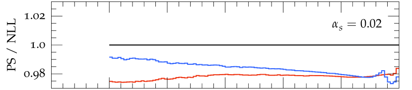
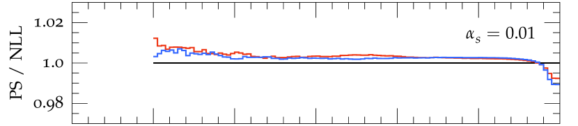
Figure 4: NLL test for various event shape observables. See the main text for details.

In this section we present numerical tests of our new algorithm. We follow the procedure outlined in Dasgupta et al. (2020) and perform a scaling of the strong coupling, while keeping the variable $\lambda=\alpha_{s}\ln v$ fixed, where $v$ is an observable whose single-emission contribution to a measurement can be parametrized in the form $v(k)=(k_{t}/Q)^{a}e^{-b|\eta_{k}|}$, see Eq. (47). In particular we analyze the event shape observables thrust, $T$ Farhi (1977), jet broadening, $B_{T}$ Catani et al. (1992), heavy jet mass, $M_{H}$, and the fractional energy correlators $FC_{1-\beta}$ Banfi et al. (2005) for $\beta=0$ and $1/2$. We also analyze the leading Lund plane declustering scale in the Cambridge algorithm, $y_{23}$, and the azimuthal angle between the two leading Lund plane declusterings, $\Delta\psi_{12}$ Dasgupta et al. (2020).

Since the running of the strong coupling will not affect the kinematics reconstruction, we keep $\alpha_{s}$ constant in this numerical test. In addition, we do not use the CMW scheme, and we work in the strict leading color approximation, $2C_{F}=C_{A}=3$. We find that this is sufficient to reproduce the dominant features of the Dire dipole shower algorithm that were observed to break NLL precision in Dasgupta et al. (2018, 2020). Figure 3 shows the azimuthal angle separation $\Delta\psi_{12}$. The predictions from Dire exhibit the same features as already shown in Dasgupta et al. (2020), and it can be seen that the deviation from a flat $\Delta\psi_{12}$ distribution does not vanish as $\alpha_{s}\to 0$. In contrast, for the Alaric algorithm we observe increasingly smaller deviations from a flat $\Delta\psi_{12}$ dependence, in agreement with NLL resummation.

Figure 4 displays the event shape observables and the leading Lund declustering scale for varying $\alpha_{s}$. In order to test for a variety of possible effects of NLL violation, we have chosen observables with different NLL contributions. In addition, we test observables with $b=0$ ($\sqrt{y_{23}}$, $B_{T}$ and $FC_{1}$), observables with $b=1/2$ ($FC_{1/2}$) and observables with $b=1$ ($1-T$, $M_{H}$). In each case we find that the deviation of the Alaric prediction from the NLL target result (modified to account for constant $\alpha_{s}$, no CMW rescaling and leading color) decreases in size proportional to the scaling in $\alpha_{s}$, as $\alpha_{s}\to 0$. At the same time, we observe large deviations of the Dire predictions from the target NLL result. It is notable that the predictions from Alaric are flat with respect to the NLL result starting at fairly small values of $-\lambda$ for most observables. For each prediction we have performed a fit to a linear function of $\alpha_{s}$ in order to extract the limit for $\alpha_{s}\to 0$. There are two noteworthy artefacts of this extrapolation: Firstly, there are bumps in the extrapolated result at large values of $\lambda$, which would not be present in the true ratio at any $\alpha_{s}<0.0025$. Second, the extrapolated result is smoother than the individual inputs, since the predictions at smaller $\alpha_{s}$ are less constraining due to their larger uncertainties. This concludes our tests of the kinematics mapping.

VI Comparison to experimental data

Figure 5: Alaric and Dire predictions in comparison to LEP data from Pfeifenschneider et al. (2000).

Figure 6: Alaric and Dire predictions in comparison to LEP data from Heister et al. (2004).

In this section we present first numerical results obtained with the Alaric final-state parton shower, as implemented in the event generation framework Sherpa Gleisberg et al. (2004, 2009); Bothmann et al. (2019). We do not perform NLO matching or multi-jet merging, and we set $C_{F}=(N_{c}^{2}-1)/(2N_{c})=4/3$ and $C_{A}=3$. All quarks are considered massless, and we implement flavor thresholds at $m_{c}=1.42$ GeV and $m_{b}=4.92$ GeV. The running coupling is evaluated at two loop accuracy, and we set $\alpha_{s}(m_{z})=0.118$. Following standard practice to improve the logarithmic accuracy of the parton shower, we employ the CMW scheme Catani et al. (1991), i.e. the soft eikonal contribution to the flavor conserving splitting functions is rescaled by $1+\alpha_{s}(t)/(2\pi)K$, where $K=(67/18-\pi^{2}/6)\,C_{A}-10/9\,T_{R}\,n_{f}$. Our results include the simulation of hadronization using the Lund string fragmentation implemented in Pythia 6.4 Sjöstrand et al. (2006) . We use the default hadronization parameters, apart from the following values: PARJ(21)=0.3, PARJ(41)=0.4, PARJ(42)=0.36 for Alaric, and PARJ(21)=0.3, PARJ(41)=0.4, PARJ(42)=0.45 for Dire. All analyses are performed with Rivet Buckley et al. (2013).

Figure 5 shows predictions from the Alaric parton shower for differential jet rates in the Durham scheme compared to experimental results from the JADE and OPAL collaborations Pfeifenschneider et al. (2000). The perturbative region is to the right of the plot, and $y\sim 2.8\cdot 10^{-3}$ corresponds to the $b$-quark mass. The simulation of nonperturbative effects dominates the predictions below $\sim 10^{-4}$. We observe fairly good agreement with the experimental data, however, we note that at moderate values of $y$ the prediction will be altered when a proper evolution of massive quark final states is included.

Figure 6 shows a comparison for event shapes measured by the ALEPH collaboration Heister et al. (2004). The perturbative region is to the right of the plot, except for the thrust distribution, where it is to the left. We notice some deviation in the predictions for the total jet broadening and for the aplanarity. They are mostly within the $2\sigma$ uncertainty of the experimental measurements. It can be expected that the simulations will improve upon including matrix-element corrections or when merging the Alaric parton shower with higher-multiplicity calculations. Deviations in the hadronization region may be associated with the treatment of $b$-quarks and $c$-quarks as massless partons.

VII Conclusions

We have presented a new parton-shower algorithm, which is closely modeled on the fixed-order subtraction formalism for identified particles by Catani and Seymour. This technique allows, for the first time in a dipole-like parton shower, to disentangle color and kinematics, at the price of introducing an azimuthal angle dependence in the splitting functions. Partial fractioning the angular radiator function and matching to the collinear limit maintains strict positivity of the evolution kernels, thus allowing a straightforward implementation without the need for explicit angular ordering. Through a suitable assignment of recoil, which is absorbed by the entire QCD multipole, we are able to show that the local kinematics mapping satisfies the criteria for NLL precision.

Several extensions of this algorithm are required: Firstly, it should be modified to include spin correlations Collins (1988); Knowles (1988a, b, 1990) and dominant sub-leading color effects Gustafson (1993); Dulat et al. (2018); Hamilton et al. (2021). A number of formally less relevant, but practically important considerations need to be addressed as well. They include the evolution for massive partons, in order to properly describe bottom and charm jet production and $b$- and $c$-quark fragmentation functions. Another open question is the extension to processes with non-trivial color dependence at Born level, such as top-quark pair production and inclusive jet or di-jet production at hadron colliders. A related, though substantially simpler problem is the treatment of processes with multiple, disconnected QCD multipoles, such as vector boson fusion in the structure function approximation, or the production of a Higgs boson in association with a hadronically decaying vector boson in the narrow width approximation. The latter cases can be handled by applying the algorithms introduced here to each QCD multipole individually, while keeping track of spin correlations among the different multipoles. Finally, we plan to extend our new algorithms to higher-orders, based on the techniques developed in Höche and Prestel (2017); Dulat et al. (2018); Gellersen et al. (2022).

Appendix A Implementation details

This appendix summarizes details of the kinematics mapping and the relations between the kinematic invariants and the evolution and splitting variables for both final-state and initial-state evolution. We limit the discussion to situations where the recoiler momentum is composed either of final-state momenta only, or of initial-state momenta only.

A.1 Final-state evolution

We will first discuss the case of a final-state emitter with a recoil momentum $\tilde{K}$ that is composed only of final-state momenta. The momentum mapping is sketched in Fig. 7 (FF). The emitting particle is labeled $i$, the emission is labeled $j$, and the color spectator is labeled $k$. The momenta $p_{i}$, $p_{j}$ and $K$ are given by Eq. (21)

$$\begin{split}p_{i}&=\,z\,\tilde{p}_{i}\;,\\ p_{j}&=\,(1-z)\,\tilde{p}_{i}+v\big{(}\tilde{K}-(1-z+2\kappa)\,\tilde{p}_{i}\big{)}+k_{\perp}\;,\\ K&=\,\tilde{K}-v\big{(}\tilde{K}-(1-z+2\kappa)\,\tilde{p}_{i}\big{)}-k_{\perp}\;,\end{split}$$ (62)

where

$${\rm k}_{\perp}^{2}=v(1-v)(1-z)\,2\tilde{p}_{i}\tilde{K}-v^{2}\tilde{K}^{2}\;,\qquad\text{and}\qquad v=\frac{\tau}{1-z}\;.$$ (63)

The particles included in the momentum $\tilde{K}$ are subjected to a Lorentz transformation, which accounts for the decay of the new recoil momentum, $K$, in a different frame. If the recoil momentum is given by a single, light-like vector, no such transformation is necessary.

$$p_{l}^{\mu}\to\Lambda^{\mu}_{\;\nu}(\tilde{K},K)\,p_{l}^{\nu}\;.$$ (64)

The momentum mapping for final-state emitters with with a recoil momentum $\tilde{K}$ composed only of initial-state momenta is sketched in Fig. 7 (FI). We define the momentum $\tilde{K}$ as incoming, i.e. $\tilde{K}_{0}>0$. This implies the replacement $v\to-v$, $\tilde{K}\to-\tilde{K}$ and $n\to-n$, leading to

$$\begin{split}p_{i}&=\,z\,\tilde{p}_{i}\;,\\ p_{j}&=\,(1-z)\,\tilde{p}_{i}+v\big{(}\tilde{K}+(1-z-2\kappa)\,\tilde{p}_{i}\big{)}+k_{\perp}\;,\\ K&=\,\tilde{K}+v\big{(}\tilde{K}+(1-z-2\kappa)\,\tilde{p}_{i}\big{)}+k_{\perp}\;,\end{split}$$ (65)

where

$${\rm k}_{\perp}^{2}=v(1+v)(1-z)\,2\tilde{p}_{i}\tilde{K}-v^{2}\tilde{K}^{2}\;,\qquad\text{and}\qquad v=\frac{\tau}{1-z}\;.$$ (66)

As in the case of a final-state spectator, the momenta defining $\tilde{K}$ are subjected to the Lorentz transformation given by Eq. (64). An additional transformation has to be applied, such as to align the momenta of both redefined beam particles, $p_{a}$ and $p_{b}$, with the beam axis. If there are no strongly interacting particles in the initial state, this can be achieved by the simple mapping

$$p_{l}^{\mu}\to\Lambda^{\mu}_{\;\nu}(p_{a}+p_{b},\tilde{p}_{a}+\tilde{p}_{b})\,p_{l}^{\nu}\;.$$ (67)

Note that this additional Lorentz transformation is applied to all particles in the event.

A.2 Initial-state evolution

Figure 7: Sketch of the momentum mapping for final-state emitters with final-state spectator (FF), final-state emitters with initial-state spectator (FI), initial-state emitters with final-state spectator (IF) and initial-state emitters with initial-state spectator (II).

For initial-state emissions, we redefine $z\to 1/z$. The momentum mapping for recoil momenta $\tilde{K}$ composed only of initial-state momenta is sketched in Fig. 7 (II). The emitting particle is labeled $i$, the emission is labeled $j$, and the color spectator is labeled $k$. We define both $\tilde{p}_{i}$ and $\tilde{K}$ as incoming, i.e. $\tilde{p}_{i,0}>0$ and $\tilde{K}_{0}>0$. The momenta $p_{i}$, $p_{j}$ and $K$ are then given by Eq. (21)

$$\begin{split}p_{i}&=\,\frac{1}{z}\,\tilde{p}_{i}\;,\\ p_{j}&=\,\frac{1-z}{z}\,\tilde{p}_{i}+v\left(\tilde{K}+\left(\frac{1-z}{z}-2\kappa\right)\tilde{p}_{i}\right)+k_{\perp}\;,\\ K&=\,\tilde{K}+v\left(\tilde{K}+\left(\frac{1-z}{z}-2\kappa\right)\tilde{p}_{i}\right)+k_{\perp}\;,\end{split}$$ (68)

where

$${\rm k}_{\perp}^{2}=v(1+v)\frac{1-z}{z}\,2\tilde{p}_{i}\tilde{K}-v^{2}\tilde{K}^{2}\;,\qquad\text{and}\qquad v=\frac{\tau}{1-z}\;.$$ (69)

As in the case of final-state evolution, the momenta defining $\tilde{K}$ are subjected to the Lorentz transformation given by Eq. (64). The complete event is then subjected to a Lorentz transformation, determined such as to align the momenta of the initial-state particles, $p_{a}$ and $p_{b}$, with the beam axis, while shifting the event rapidity to $y=\tilde{y}-{\rm sgn}(p_{i,z})\ln\sqrt{z}$ and preserving the azimuthal orientation of the event.

The momentum mapping for initial-state emitters with a recoil momentum $\tilde{K}$ composed only of final-state momenta is sketched in Fig. 7 (IF). The momenta $p_{i}$, $p_{j}$ and $K$ are given by

$$\begin{split}p_{i}&=\,\frac{1}{z}\,\tilde{p}_{i}\;,\\ p_{j}&=\,\frac{1-z}{z}\,\tilde{p}_{i}+v\left(\tilde{K}-\left(\frac{1-z}{z}+2\kappa\right)\tilde{p}_{i}\right)+k_{\perp}\;,\\ K&=\,\tilde{K}-v\left(\tilde{K}-\left(\frac{1-z}{z}+2\kappa\right)\tilde{p}_{i}\right)-k_{\perp}\;,\end{split}$$ (70)

where

$${\rm k}_{\perp}^{2}=v(1-v)\frac{1-z}{z}\,2\tilde{p}_{i}\tilde{K}-v^{2}\tilde{K}^{2}\;,\qquad\text{and}\qquad v=\frac{\tau}{1-z}\;.$$ (71)

The particles included in the momentum $\tilde{K}$ are subjected to a Lorentz transformation, which accounts for the decay of the new recoil momentum, $K$, in a different frame. As in the case of final-state evolution, this can be achieved by applying the Lorentz transformation in Eq. (64). If the recoil momentum is given by a single, light-like vector, no transformation is needed.

Appendix B Phase-space factorization

This appendix summarizes details on the phase-space factorization for both final-state and initial-state evolution. The case of final-state emitter and initial-state recoiler was discussed in Sec. III, and we do not repeat it here.

B.1 Final-state emitter and final-state recoiler

This case covers electroweak decays of a color-charged resonance, such as the top quark. We start from

$${\rm d}\Phi_{3}(p_{i},p_{j},K;Q)={\rm d}\Phi_{2}(p_{i},n;Q)\,\frac{{\rm d}n^{2}}{2\pi}\,{\rm d}\Phi_{2}(p_{j},K;n)$$ (72)

The generic frame-independent form of the two-particle phase space is given in Eq. (30). We perform all transformations in the rest frame of $n$, where we have the simple relations

$$E_{i}=z\,\frac{\tilde{p}_{i}\tilde{K}}{\sqrt{n^{2}}}\;,\qquad E_{j}=(1-z)\,\frac{\tilde{p}_{i}\tilde{K}}{\sqrt{n^{2}}}\;,\qquad E_{K}=(1-z+2\kappa)\,\frac{\tilde{p}_{i}\tilde{K}}{\sqrt{n^{2}}}\;,\qquad\text{and}\qquad n^{2}=2\tilde{p}_{i}\tilde{K}\,(1-z+\kappa)\;.$$ (73)

Using the following identity for the polar angle $\theta_{j}$ of the emission,

$$1-\cos\theta_{j}^{\,i}=-2v\,\frac{1-z+\kappa}{1-z}\;,$$ (74)

we find the first two-particle decay phase space to be

$${\rm d}\Phi_{2}(p_{j},K;n)=\frac{1}{16\pi^{2}}\,{\rm d}v\,\frac{{\rm d}\phi_{j}^{(n)}}{2\pi}\;.$$ (75)

Analogous to Eq. (34), we can write ${\rm d}n^{2}=2\tilde{p}_{i}\tilde{K}\,{\rm d}z$. Finally, we rewrite the second two-particle decay phase space

$${\rm d}\Phi_{2}(p_{i},n;Q)=\frac{1}{16\pi^{2}}\frac{z}{2(1-z+\kappa)}\,{\rm d}\cos\theta_{i}^{(n)}\,\frac{{\rm d}\phi_{i}^{(n)}}{2\pi}\;.$$ (76)

In order to obtain a factorization formula, this must be mapped to the Born phase space, which is given by ${\rm d}\Phi_{2}(\tilde{p}_{i},\tilde{K};Q)$. The angular integrals in Eq. (76) are identical when working in the rest frame of the momentum $n$, which leads to the relation ${\rm d}\Phi_{2}(p_{i},n;Q)=z\;{\rm d}\Phi_{2}(\tilde{p}_{i},\tilde{q}_{i};\tilde{K})$. Combining all of the above, we find the single-emission phase space element

$${\rm d}\Phi_{+1}^{\rm(FF)}(\tilde{K};\tilde{p}_{1},\ldots,\tilde{p}_{j-1},\tilde{p}_{j+1},\ldots,\tilde{p}_{n};p_{j})=\frac{2z\tilde{p}_{i}\tilde{K}}{16\pi^{2}}\,{\rm d}v\,{\rm d}z\,\frac{{\rm d}\phi}{2\pi}\;.$$ (77)

B.2 Initial-state emitter and final-state recoiler

This case covers hadroproduction of a colorless final state, in particular Drell-Yan lepton pair production. We start from the factorization formula

$${\rm d}\Phi_{2}(p_{j},K;Q+p_{i})={\rm d}\Phi_{2}(p_{j},K;n)\,\frac{{\rm d}n^{2}}{2\pi}\,{\rm d}\Phi_{1}(n;Q+p_{i})$$ (78)

The generic frame-independent form of the two-particle phase space is given in Eq. (30). Again, we perform all transformations in the rest frame of $n$, leading to the relations in Eq. (73). Using Eq. (74) for the polar angle $\theta_{j}$ of the emission, we find the two-particle decay phase space in Eq. (75). Analogous to Eq. (34), we can write ${\rm d}n^{2}=2\tilde{p}_{i}\tilde{K}\,{\rm d}z$. The one-particle production phase space is given by

$${\rm d}\Phi_{1}(n;Q+p_{i})=2\pi\,\delta(n^{2}-(Q+p_{i})^{2})\;.$$ (79)

In order to obtain a factorization formula, this is mapped to the Born phase space, leading to ${\rm d}\Phi_{1}(n;Q+p_{i})=1/z\;{\rm d}\Phi_{2}(\tilde{K};Q+\tilde{p}_{i})$. Combining all of the above, we obtain the single-emission phase space element

$${\rm d}\Phi_{+1}^{\rm(IF)}(\tilde{K};\tilde{p}_{1},\ldots,\tilde{p}_{j-1},\tilde{p}_{j+1},\ldots,\tilde{p}_{n};p_{j})=\frac{2\tilde{p}_{i}\tilde{K}}{16\pi^{2}}\,{\rm d}v\,\frac{{\rm d}x}{x}\,\frac{{\rm d}\phi}{2\pi}\;.$$ (80)

B.3 Initial-state emitter and initial-state recoiler

This case covers deep inelastic scattering. We start from the two-particle phase space

$${\rm d}\Phi_{2}(p_{j},Q;K+p_{i})\;.$$ (81)

Its generic, frame-independent form is given in Eq. (30). We perform all transformations in the rest frame of $n$, where we have the relations in Eq. (31). Next we insert the identity

$$1=\int{\rm d}x\;\delta\left(x-\frac{\tilde{p}_{i}\tilde{K}}{p_{i}n}\right)=\int{\rm d}x\;\frac{2\tilde{p}_{i}\tilde{K}}{x}\,\delta\left(2\tilde{p}_{i}\tilde{K}-(p_{i}+p_{j})n\right)=\int{\rm d}x\;\frac{2\tilde{p}_{i}\tilde{K}}{x}\,\delta\left((\tilde{p}_{i}+\tilde{K})^{2}-Q^{2}\right)\;.$$ (82)

In order to obtain a factorization formula, this is mapped to the Born phase space as ${\rm d}\Phi_{1}(\tilde{Q};\tilde{p}_{i}+\tilde{K})=2\pi\,\delta(\tilde{Q}^{2}-(\tilde{p}_{i}+\tilde{K})^{2})$. Combining all of the above, we obtain the single-emission phase space element

$${\rm d}\Phi_{+1}^{\rm(IF)}(\tilde{K};\tilde{p}_{1},\ldots,\tilde{p}_{j-1},\tilde{p}_{j+1},\ldots,\tilde{p}_{n};p_{j})=\frac{2\tilde{p}_{i}\tilde{K}}{16\pi^{2}}\,{\rm d}v\,\frac{{\rm d}x}{x}\,\frac{{\rm d}\phi}{2\pi}\;.$$ (83)

Appendix C Monte-Carlo counterterms for MC@NLO matching

To match a parton shower to NLO calculations in dimensional regularization based on the MC@NLO algorithm Frixione and Webber (2002), the integral of the splitting functions must be known in $D=4-2\varepsilon$ dimensions. Since our new parton shower is modeled on the Catani-Seymour identified particle subtraction, we can utilize the techniques developed in Höche et al. (2019); Liebschner (2020). By means of a suitable identification of the radiating color multipole, this allows us to treat the problem of standard final-state evolution, resonant particle production, color singlet production at hadron colliders, deep-inelastic scattering, etc. on the same footing.

Here we will limit ourselves to listing the main changes with respect to Höche et al. (2019); Liebschner (2020) that are needed in order to implement the algorithm. For details on the respective phase-space integrals, and on the basis of the subtraction technique, we refer the reader to Catani and Seymour (1997). Details on the implementation of MC@NLO can be found in Frixione and Webber (2002); Höche et al. (2012).

C.1 Final-state emitter

By combining the integrated splitting function with the collinear mass factorization counterterms, we can derive a combined integrated subtraction term for identified parton production with a partonic fragmentation function Höche et al. (2019); Liebschner (2020)

$$\int_{m+1}\mathrm{d}\sigma^{S}+\int_{m}\mathrm{d}\sigma^{C}=\frac{1}{2}\sum_{i=g,q,\bar{q}}\sum_{\tilde{\imath}=1}^{m}\int_{0}^{1}\frac{\mathrm{d}z}{z^{2-2\epsilon}}\int_{m}\mathrm{d}\sigma^{B}(p_{1},\dots,\frac{p_{i}}{z},\dots,p_{m})\otimes\hat{\mathbf{I}}_{\tilde{\imath}i}^{\rm(FS)}\;,$$ (84)

where the $\otimes$ stands for spin and color correlations. In the $\overline{\mathrm{MS}}$ scheme, the insertion operator is given by

$$\hat{\mathbf{I}}_{\tilde{\imath}i}^{\rm(FS)}=-\frac{\alpha_{s}}{2\pi}\frac{1}{\Gamma(1-\epsilon)}\Bigg{\{}\sum_{k=1,k\neq\tilde{\imath}}^{m}\frac{\mathbf{T}_{\tilde{\imath}}\mathbf{T}_{k}}{\mathbf{T}_{\tilde{\imath}}^{2}}\left(\frac{4\pi\mu^{2}(p_{k}n)}{2(p_{i}p_{k})(p_{i}n)}\right)^{\epsilon}\hat{\mathcal{V}}_{\tilde{\imath},i}(z;\epsilon;p_{i},p_{k},n)-\delta_{\tilde{\imath}i}\frac{1}{\epsilon}\left(\frac{4\pi\mu^{2}}{\mu_{F}^{2}}\right)^{\epsilon}P_{\tilde{\imath}i}(z)\Bigg{\}}~{}.$$ (85)

The explicit pole in $\epsilon$, originating from the renormalization of the perturbative fragmentation function, cancels against the corresponding pole in $\bar{\mathcal{V}}_{\tilde{\imath},i}$. The remainder can be split into three contributions:

$$\hat{\mathbf{I}}_{\tilde{\imath}i}^{\rm(FS)}=\delta(1-z)\mathbf{I}_{\tilde{\imath}i}+\mathbf{P}_{\tilde{\imath}i}+\mathbf{H}_{\tilde{\imath}i}~{}.$$ (86)

The singularities in the virtual corrections are canceled by the insertion operator present for standard final-state dipoles with final-state spectator Catani and Seymour (1997)

$$\mathbf{I}_{\tilde{\imath}i}(p_{1},\dots,p_{i},\dots,p_{m};\epsilon)=-\frac{\alpha_{s}}{2\pi}\frac{1}{\Gamma(1-\epsilon)}\sum_{k=1,k\neq\tilde{\imath}}^{m}\frac{\mathbf{T}_{\tilde{\imath}}\mathbf{T}_{k}}{\mathbf{T}_{\tilde{\imath}}^{2}}\left(\frac{4\pi\mu^{2}(p_{k}n)}{2(p_{i}p_{k})(p_{i}n)}\right)^{\epsilon}\mathcal{V}_{\tilde{\imath}i}(\epsilon)\;.$$ (87)

Employing color conservation and expanding through $\mathcal{O}(\epsilon)$, the remaining two operators read Höche et al. (2019); Liebschner (2020)

$$\mathbf{P}_{\tilde{\imath}i}(p_{1},\dots,\frac{p_{i}}{z},\dots,p_{m};z;\mu_{F})=\frac{\alpha_{s}}{2\pi}\sum_{k=1,k\neq\tilde{\imath}}^{m}\frac{\mathbf{T}_{\tilde{\imath}}\mathbf{T}_{k}}{\mathbf{T}_{\tilde{\imath}}^{2}}\ln\frac{z^{2}\mu_{F}^{2}(p_{k}n)}{2(p_{i}p_{k})(p_{i}n)}\delta_{\tilde{\imath}i}P_{\tilde{\imath}i}(z)$$ (88)

and

$$\mathbf{H}_{\tilde{\imath}i}(p_{1},\dots,p_{i},\dots,p_{m};n;z)=-\frac{\alpha_{s}}{2\pi}\sum_{k=1,k\neq\tilde{\imath}}^{m}\frac{\mathbf{T}_{\tilde{\imath}}\mathbf{T}_{k}}{\mathbf{T}_{\tilde{\imath}}^{2}}\left[\tilde{K}^{\tilde{\imath}i}(z)+\bar{K}^{\tilde{\imath}i}(z)+2P_{\tilde{\imath}i}(z)\ln z+\hat{\mathcal{L}}^{\tilde{\imath}i}(z;p_{i},p_{k},n)\right]~{}.$$ (89)

Finally, an integration over $p_{i}$ has to be performed. Following Refs. Höche et al. (2019); Liebschner (2020) we replace the integration over $p_{i}$ by an integration over $\tilde{p}_{i}$. This leads to a Jacobian of $z^{2-2\epsilon}$, canceling the prefactor in Eq. (84). Consequently, the differential Born cross-section $\mathrm{d}\sigma^{B}$ decouples from the $z$ integration and we obtain

$$\sum_{\tilde{\imath}=1}^{m}\int\frac{\mathrm{d}^{D}p_{i}}{(2\pi)^{D-1}}\delta(p_{i}^{2})\sigma^{I}(p_{i})=\sum_{\tilde{\imath}=1}^{m}\int_{m}\mathrm{d}\sigma^{B}(p_{1},\dots,p_{m})\otimes\int_{0}^{1}\mathrm{d}z\;\frac{1}{2}\sum_{i=g,q,\bar{q}}\hat{\mathbf{I}}_{\tilde{\imath}i}\;.$$ (90)

The integral over $\sum_{i}\mathbf{P}_{\tilde{\imath}i}$ vanishes, because $\sum_{i}P_{\tilde{i}i}$ is a pure plus distribution. The other two $z$-integrals can be evaluated directly, because $\tilde{p}_{i}$ is $z$-independent. In particular, the integral of the $\mathbf{I}_{\tilde{\imath}}$ operator is trivial. The integral over the $\mathbf{H}_{\tilde{\imath}i}$ operator is given by a modified form of the result in Höche et al. (2019); Liebschner (2020). We note that the arguments of the dilogarithms depend only on the angle and velocity of $l_{ik}$ as defined in Eq. (39), see Appendix B in Catani and Seymour (1997). Using the following substitution in Eq. (B.9) in Catani and Seymour (1997)

$$1-v\cos\chi\to\frac{n^{2}\,l_{ik}p_{i}}{(p_{i}n)(l_{ik}n)}\;,\qquad 1-v^{2}\to\frac{n^{2}l_{ik}^{2}}{(l_{ik}n)^{2}}\;,$$ (91)

we therefore obtain

$$\begin{split}&\int_{0}^{1}\mathrm{d}{z}\,\mathbf{H}_{\tilde{\imath}i}(p_{1},\dots,p_{i},\dots,p_{m};n;z)\\ &\qquad=-\frac{\alpha_{s}}{2\pi}\sum_{k=1,k\neq\tilde{\imath}}^{m}\frac{\mathbf{T}_{\tilde{\imath}}\mathbf{T}_{k}}{\mathbf{T}_{\tilde{\imath}}^{2}}\Bigg{\{}\;\mathcal{K}^{\tilde{\imath}i}+\delta_{\tilde{\imath}i}\,\mathrm{Li}_{2}\bigg{(}1-\frac{2\tilde{p}_{i}\tilde{p}_{k}\,\tilde{K}^{2}}{(\tilde{p}_{i}\tilde{K})(\tilde{p}_{k}\tilde{K})}\bigg{)}-\int_{0}^{1}\mathrm{d}z\,P^{\tilde{\imath}i}_{\rm reg}(z)\ln\frac{(p_{i}p_{k})n^{2}}{2(p_{i}n)(p_{k}n)}\;\Bigg{\}}\;,\end{split}$$ (92)

where the integral $\mathcal{K}^{\tilde{\imath}i}$ is defined as

$$\mathcal{K}^{\tilde{\imath}i}=\int_{0}^{1}\mathrm{d}z~{}\Big{(}\bar{K}^{\tilde{\imath}i}(z)+\tilde{K}^{\tilde{\imath}i}(z)+2P_{\tilde{\imath}i}(z)\ln z\Big{)}\;.$$ (93)

In general, the last term of Eq. (92) must be computed numerically, as $n$ implicitly depends on $z$, see Eq. (17).

C.2 Initial-state emitter

As in the case of a final-state emitter, the case of an initial state emitter is treated in the same manner as in Höche et al. (2019); Liebschner (2020). The sum of the subtraction terms and the collinear counterterms is given by

$$\int_{m+1}\mathrm{d}\sigma^{S}+\int_{m}\mathrm{d}\sigma^{C}=\sum_{\tilde{i}=g,q,\bar{q}}\int_{0}^{1}\mathrm{d}x\int_{m}\mathrm{d}\sigma^{B}(p_{1},\dots,xp_{i},\dots,p_{m})\otimes\hat{\mathbf{I}}_{i\tilde{\imath}}^{\rm(IS)}\;,$$ (94)

where the $\otimes$ again stands for spin and color correlations. In the $\overline{\rm MS}$ scheme, the insertion operator is given by

$$\hat{\mathbf{I}}_{i\tilde{\imath}}^{\rm(IS)}=\delta(1-z)\mathbf{I}_{i\tilde{\imath}}+\mathbf{P}_{i\tilde{\imath}}+\mathbf{K}_{i\tilde{\imath}}\;.$$ (95)

The operator $\mathbf{I}_{i\tilde{\imath}}$ is obtained by replacing $k\to\tilde{k}$ in Eq. (87). The $\mathbf{K}$ operator can be written as

$$\mathbf{K}_{i\tilde{\imath}}(p_{1},\ldots,p_{m};p_{i},n,x)=-\frac{\alpha_{s}}{2\pi}\sum_{\tilde{b}=1}^{m}\frac{\mathbf{T}_{\tilde{k}}\mathbf{T}_{\tilde{\imath}}}{\mathbf{T}_{\tilde{\imath}}^{2}}\left[\;\bar{K}^{i,\tilde{\imath}}(x)+\tilde{K}^{i,\tilde{\imath}}(x)+\mathcal{L}^{i,\tilde{\imath}}(x;p_{i},\tilde{p}_{k},n)\;\right]\;.$$ (96)

This result can be derived from Eq. (89) by using the known expressions for the breaking of the Gribov-Lipatov relation at NLO QCD, see Sec. 6.4 of Curci et al. (1980). All remaining components of the subtraction formulae can be found in Appendix C of Catani and Seymour (1997).

References

- Buckley et al. (2011) A. Buckley et al., Phys. Rept. 504, 145 (2011), arXiv:1101.2599 [hep-ph] .
- Campbell et al. (2022) J. M. Campbell et al., in 2022 Snowmass Summer Study (2022) arXiv:2203.11110 [hep-ph] .
- Dokshitzer (1977) Y. L. Dokshitzer, Sov. Phys. JETP 46, 641 (1977).
- Gribov and Lipatov (1972) V. N. Gribov and L. N. Lipatov, Sov. J. Nucl. Phys. 15, 438 (1972).
- Lipatov (1975) L. N. Lipatov, Sov. J. Nucl. Phys. 20, 94 (1975).
- Altarelli and Parisi (1977) G. Altarelli and G. Parisi, Nucl. Phys. B126, 298 (1977).
- Lönnblad (1992) L. Lönnblad, Comput. Phys. Commun. 71, 15 (1992).
- Kharraziha and Lönnblad (1998) H. Kharraziha and L. Lönnblad, JHEP 03, 006 (1998), hep-ph/9709424 .
- Jung and Salam (2001) H. Jung and G. P. Salam, Eur. Phys. J. C19, 351 (2001), hep-ph/0012143 .
- Webber (1984) B. R. Webber, Nucl. Phys. B238, 492 (1984).
- Bengtsson et al. (1986) M. Bengtsson, T. Sjöstrand, and M. van Zijl, Z. Phys. C32, 67 (1986).
- Bengtsson and Sjöstrand (1987a) M. Bengtsson and T. Sjöstrand, Nucl. Phys. B289, 810 (1987a).
- Marchesini and Webber (1988) G. Marchesini and B. R. Webber, Nucl. Phys. B310, 461 (1988).
- Andersson et al. (1990) B. Andersson, G. Gustafson, and L. Lönnblad, Nucl. Phys. B339, 393 (1990).
- Mueller (1981) A. H. Mueller, Phys. Lett. B104, 161 (1981).
- Ermolaev and Fadin (1981) B. I. Ermolaev and V. S. Fadin, JETP Lett. 33, 269 (1981).
- Dokshitzer et al. (1982a) Y. L. Dokshitzer, V. S. Fadin, and V. A. Khoze, Phys. Lett. B 115, 242 (1982a).
- Dokshitzer et al. (1982b) Y. L. Dokshitzer, V. S. Fadin, and V. A. Khoze, Z. Phys. C15, 325 (1982b).
- Dokshitzer et al. (1983) Y. L. Dokshitzer, V. S. Fadin, and V. A. Khoze, Z. Phys. C 18, 37 (1983).
- Bassetto et al. (1982) A. Bassetto, M. Ciafaloni, G. Marchesini, and A. H. Mueller, Nucl. Phys. B207, 189 (1982).
- Webber (1986) B. Webber, Ann. Rev. Nucl. Part. Sci. 36, 253 (1986).
- Bengtsson and Sjöstrand (1987b) M. Bengtsson and T. Sjöstrand, Phys. Lett. B185, 435 (1987b).
- Collins (1988) J. C. Collins, Nucl.Phys. B304, 794 (1988).
- Knowles (1988a) I. Knowles, Nucl.Phys. B304, 767 (1988a).
- Knowles (1988b) I. Knowles, Nucl.Phys. B310, 571 (1988b).
- Knowles (1990) I. Knowles, Comput.Phys.Commun. 58, 271 (1990).
- Frixione and Webber (2002) S. Frixione and B. R. Webber, JHEP 06, 029 (2002), hep-ph/0204244 .
- Nason (2004) P. Nason, JHEP 11, 040 (2004), hep-ph/0409146 .
- Frixione et al. (2007) S. Frixione, P. Nason, and C. Oleari, JHEP 11, 070 (2007), arXiv:0709.2092 [hep-ph] .
- Alioli et al. (2010) S. Alioli, P. Nason, C. Oleari, and E. Re, JHEP 06, 043 (2010), arXiv:1002.2581 [hep-ph] .
- Höche et al. (2011) S. Höche, F. Krauss, M. Schönherr, and F. Siegert, JHEP 04, 024 (2011), arXiv:1008.5399 [hep-ph] .
- Höche et al. (2012) S. Höche, F. Krauss, M. Schönherr, and F. Siegert, JHEP 09, 049 (2012), arXiv:1111.1220 [hep-ph] .
- Alwall et al. (2014) J. Alwall, R. Frederix, S. Frixione, V. Hirschi, F. Maltoni, O. Mattelaer, H.-S. Shao, T. Stelzer, P. Torrielli, and M. Zaro, JHEP 07, 079 (2014), arXiv:1405.0301 [hep-ph] .
- Catani et al. (2001) S. Catani, F. Krauss, R. Kuhn, and B. R. Webber, JHEP 11, 063 (2001), hep-ph/0109231 .
- Lönnblad (2002) L. Lönnblad, JHEP 05, 046 (2002), hep-ph/0112284 .
- Krauss (2002) F. Krauss, JHEP 08, 015 (2002), hep-ph/0205283 .
- Alwall et al. (2008) J. Alwall et al., Eur. Phys. J. C53, 473 (2008), arXiv:0706.2569 [hep-ph] .
- Höche et al. (2009) S. Höche, F. Krauss, S. Schumann, and F. Siegert, JHEP 05, 053 (2009), arXiv:0903.1219 [hep-ph] .
- Lönnblad and Prestel (2012) L. Lönnblad and S. Prestel, JHEP 03, 019 (2012), arXiv:1109.4829 [hep-ph] .
- Gehrmann et al. (2013) T. Gehrmann, S. Höche, F. Krauss, M. Schönherr, and F. Siegert, JHEP 01, 144 (2013), arXiv:1207.5031 [hep-ph] .
- Höche et al. (2013) S. Höche, F. Krauss, M. Schönherr, and F. Siegert, JHEP 04, 027 (2013), arXiv:1207.5030 [hep-ph] .
- Frederix and Frixione (2012) R. Frederix and S. Frixione, JHEP 12, 061 (2012), arXiv:1209.6215 [hep-ph] .
- Lönnblad and Prestel (2013) L. Lönnblad and S. Prestel, JHEP 03, 166 (2013), arXiv:1211.7278 [hep-ph] .
- Plätzer (2013) S. Plätzer, JHEP 08, 114 (2013), arXiv:1211.5467 [hep-ph] .
- Nagy and Soper (2005) Z. Nagy and D. E. Soper, JHEP 10, 024 (2005), hep-ph/0503053 .
- Nagy and Soper (2006) Z. Nagy and D. E. Soper, (2006), hep-ph/0601021 .
- Schumann and Krauss (2008) S. Schumann and F. Krauss, JHEP 03, 038 (2008), arXiv:0709.1027 [hep-ph] .
- Giele et al. (2008) W. T. Giele, D. A. Kosower, and P. Z. Skands, Phys. Rev. D78, 014026 (2008), arXiv:0707.3652 [hep-ph] .
- Plätzer and Gieseke (2011) S. Plätzer and S. Gieseke, JHEP 01, 024 (2011), arXiv:0909.5593 [hep-ph] .
- Höche and Prestel (2015) S. Höche and S. Prestel, Eur. Phys. J. C75, 461 (2015), arXiv:1506.05057 [hep-ph] .
- Fischer et al. (2016) N. Fischer, S. Prestel, M. Ritzmann, and P. Skands, Eur. Phys. J. C 76, 589 (2016), arXiv:1605.06142 [hep-ph] .
- Cabouat and Sjöstrand (2018) B. Cabouat and T. Sjöstrand, Eur. Phys. J. C78, 226 (2018), arXiv:1710.00391 [hep-ph] .
- Dasgupta et al. (2018) M. Dasgupta, F. A. Dreyer, K. Hamilton, P. F. Monni, and G. P. Salam, JHEP 09, 033 (2018), [Erratum: JHEP 03, 083 (2020)], arXiv:1805.09327 [hep-ph] .
- Dasgupta et al. (2020) M. Dasgupta, F. A. Dreyer, K. Hamilton, P. F. Monni, G. P. Salam, and G. Soyez, Phys. Rev. Lett. 125, 052002 (2020), arXiv:2002.11114 [hep-ph] .
- Nagy and Soper (2012) Z. Nagy and D. E. Soper, JHEP 1206, 044 (2012), arXiv:1202.4496 [hep-ph] .
- Plätzer and Sjödahl (2012) S. Plätzer and M. Sjödahl, JHEP 07, 042 (2012), arXiv:1201.0260 [hep-ph] .
- Nagy and Soper (2014) Z. Nagy and D. E. Soper, JHEP 06, 097 (2014), arXiv:1401.6364 [hep-ph] .
- Nagy and Soper (2015) Z. Nagy and D. E. Soper, JHEP 07, 119 (2015), arXiv:1501.00778 [hep-ph] .
- Plätzer et al. (2018) S. Plätzer, M. Sjodahl, and J. Thorén, JHEP 11, 009 (2018), arXiv:1808.00332 [hep-ph] .
- Isaacson and Prestel (2019) J. Isaacson and S. Prestel, Phys. Rev. D 99, 014021 (2019), arXiv:1806.10102 [hep-ph] .
- Nagy and Soper (2019a) Z. Nagy and D. E. Soper, Phys. Rev. D 100, 074005 (2019a), arXiv:1908.11420 [hep-ph] .
- Nagy and Soper (2019b) Z. Nagy and D. E. Soper, Phys. Rev. D 99, 054009 (2019b), arXiv:1902.02105 [hep-ph] .
- Forshaw et al. (2019) J. R. Forshaw, J. Holguin, and S. Plätzer, JHEP 08, 145 (2019), arXiv:1905.08686 [hep-ph] .
- Höche and Reichelt (2021) S. Höche and D. Reichelt, Phys. Rev. D 104, 034006 (2021), arXiv:2001.11492 [hep-ph] .
- De Angelis et al. (2021) M. De Angelis, J. R. Forshaw, and S. Plätzer, Phys. Rev. Lett. 126, 112001 (2021), arXiv:2007.09648 [hep-ph] .
- Holguin et al. (2021) J. Holguin, J. R. Forshaw, and S. Plätzer, Eur. Phys. J. C 81, 364 (2021), arXiv:2011.15087 [hep-ph] .
- Hamilton et al. (2021) K. Hamilton, R. Medves, G. P. Salam, L. Scyboz, and G. Soyez, JHEP 03, 041 (2021), arXiv:2011.10054 [hep-ph] .
- Höche et al. (2018) S. Höche, D. Reichelt, and F. Siegert, JHEP 01, 118 (2018), arXiv:1711.03497 [hep-ph] .
- Bewick et al. (2020) G. Bewick, S. Ferrario Ravasio, P. Richardson, and M. H. Seymour, JHEP 04, 019 (2020), arXiv:1904.11866 [hep-ph] .
- Forshaw et al. (2020) J. R. Forshaw, J. Holguin, and S. Plätzer, JHEP 09, 014 (2020), arXiv:2003.06400 [hep-ph] .
- van Beekveld et al. (2022) M. van Beekveld, S. Ferrario Ravasio, G. P. Salam, A. Soto-Ontoso, G. Soyez, and R. Verheyen, JHEP 11, 019 (2022), arXiv:2205.02237 [hep-ph] .
- Catani and Seymour (1997) S. Catani and M. H. Seymour, Nucl. Phys. B485, 291 (1997), hep-ph/9605323 .
- Höche and Prestel (2017) S. Höche and S. Prestel, Phys. Rev. D96, 074017 (2017), arXiv:1705.00742 [hep-ph] .
- Dulat et al. (2018) F. Dulat, S. Höche, and S. Prestel, Phys. Rev. D98, 074013 (2018), arXiv:1805.03757 [hep-ph] .
- Gleisberg et al. (2004) T. Gleisberg, S. Höche, F. Krauss, A. Schälicke, S. Schumann, and J. Winter, JHEP 02, 056 (2004), hep-ph/0311263 .
- Gleisberg et al. (2009) T. Gleisberg, S. Höche, F. Krauss, M. Schönherr, S. Schumann, F. Siegert, and J. Winter, JHEP 02, 007 (2009), arXiv:0811.4622 [hep-ph] .
- Bothmann et al. (2019) E. Bothmann et al. (Sherpa), SciPost Phys. 7, 034 (2019), arXiv:1905.09127 [hep-ph] .
- Hamilton et al. (2022) K. Hamilton, A. Karlberg, G. P. Salam, L. Scyboz, and R. Verheyen, JHEP 03, 193 (2022), arXiv:2111.01161 [hep-ph] .
- Bassetto et al. (1983) A. Bassetto, M. Ciafaloni, and G. Marchesini, Phys. Rept. 100, 201 (1983).
- Ellis et al. (1996) R. K. Ellis, W. J. Stirling, and B. R. Webber, QCD and collider physics, 1st ed., Vol. 8 (Cambridge Monogr. Part. Phys. Nucl. Phys. Cosmol., 1996) p. 435.
- Sudakov (1956) V. V. Sudakov, Sov. Phys. JETP 3, 65 (1956).
- Sjöstrand et al. (2006) T. Sjöstrand, S. Mrenna, and P. Skands, JHEP 05, 026 (2006), hep-ph/0603175 .
- Catani et al. (1993) S. Catani, L. Trentadue, G. Turnock, and B. R. Webber, Nucl. Phys. B407, 3 (1993).
- Banfi et al. (2005) A. Banfi, G. P. Salam, and G. Zanderighi, JHEP 03, 073 (2005), hep-ph/0407286 .
- Schönherr and Krauss (2008) M. Schönherr and F. Krauss, JHEP 12, 018 (2008), arXiv:0810.5071 [hep-ph] .
- Nagy and Soper (2020) Z. Nagy and D. E. Soper, (2020), arXiv:2011.04777 [hep-ph] .
- Farhi (1977) E. Farhi, Phys. Rev. Lett. 39, 1587 (1977).
- Catani et al. (1992) S. Catani, G. Turnock, and B. R. Webber, Phys. Lett. B 295, 269 (1992).
- Pfeifenschneider et al. (2000) P. Pfeifenschneider et al. (JADE and OPAL), Eur. Phys. J. C17, 19 (2000), hep-ex/0001055 .
- Heister et al. (2004) A. Heister et al. (ALEPH), Eur. Phys. J. C35, 457 (2004).
- Catani et al. (1991) S. Catani, B. R. Webber, and G. Marchesini, Nucl. Phys. B349, 635 (1991).
- Chahal and Krauss (2022) G. S. Chahal and F. Krauss, SciPost Phys. 13, 019 (2022), arXiv:2203.11385 [hep-ph] .
- Buckley et al. (2013) A. Buckley et al., Comput.Phys.Commun. 184, 2803 (2013), arXiv:1003.0694 [hep-ph] .
- Gustafson (1993) G. Gustafson, Nucl. Phys. B 392, 251 (1993).
- Gellersen et al. (2022) L. Gellersen, S. Höche, and S. Prestel, Phys. Rev. D 105, 114012 (2022), arXiv:2110.05964 [hep-ph] .
- Höche et al. (2019) S. Höche, S. Liebschner, and F. Siegert, Eur. Phys. J. C 79, 728 (2019), arXiv:1807.04348 [hep-ph] .
- Liebschner (2020) S. Liebschner, PhD thesis, (2020), CERN-THESIS-2020-126.
- Curci et al. (1980) G. Curci, W. Furmanski, and R. Petronzio, Nucl. Phys. B175, 27 (1980).