Automated Market Making and Loss-Versus-Rebalancing

Abstract

Automated market making (AMM) protocols such as Uniswap have recently emerged as an alternative to the most common market structure for electronic trading, the limit order book. Relative to limit order books, AMMs are both more computationally efficient and do not require the participation of active market making intermediaries such as high frequency traders. As such, AMMs have emerged as the dominant market mechanism for trust-less decentralized exchanges (DEXs) implemented through smart contracts on programmable blockchain platforms such as Ethereum. In cryptocurrency markets, the aggregate trading volume on the Uniswap DEX exceeds that of the much better known Coinbase centralized exchange.

We develop a model the underlying economics of AMMs from the perspective of their passive liquidity providers (LPs). Our central contribution is a ‘‘Black-Scholes formula for AMMs’’. Like the Black-Scholes formula, we consider the return to LPs once market risk has been hedged. We identify the main adverse selection cost incurred by LPs, which we call ‘‘loss-versus-rebalancing’’ (LVR, pronounced ‘‘lever’’). LVR captures costs incurred by AMM LPs due to stale prices that are picked off by better informed arbitrageurs. In a continuous time Black-Scholes setting, we are able to derive closed-form expressions for this adverse selection cost, for all automated market makers, including constant function market makers and those featuring concentrated liquidity (e.g., Uniswap v3). Qualitatively, we highlight the main forces that drive AMM LP returns, including asset characteristics (volatility) and AMM characteristics (curvature / marginal liquidity). Quantitatively, we illustrate how our model’s expressions for LP returns match actual LP returns for the Uniswap v2 WETH-USDC trading pair. Our model provides tradable insight into both the ex ante and ex post assessment of AMM LP investment decisions. LVR can also inform the design of the next generation of DEX market mechanisms — in fact, in the short time since our work has been released, ‘‘LVR mitigation’’ has already emerged as the dominant challenge among practitioners in the AMM protocol designer community.

1 Introduction

In recent years, automated market makers (AMMs) have emerged as the dominant mechanism for decentralized exchange on blockchains. Most (but not all) of the deployed AMMs have the form of a constant function market maker (CFMM) such as Uniswap (Adams et al., 2020, 2021). Compared to electronic limit order books (LOBs), which are the dominant market structure for traditional, centralized exchange-based electronic markets, CFMMs offer some advantages. First of all, they are efficient computationally. They have minimal storage needs, and matching computations can be done quickly, typically via constant-time closed-form algebraic computations. In an LOB, on the other hand, matching engine calculations may involve complex data structures and computations that scale with the number of orders. Thus, CFMMs are uniquely suited to the severely computation- and storage-constrained environment of the blockchain. Second, LOBs are not well-suited to a ‘‘long-tail’’ of illiquid assets. This is because they require the participation of active market makers. In contrast, AMMs mainly rely on passive liquidity providers (LPs).

The goal of this paper is to understand the returns to providing liquidity in an AMM, in a manner which is inspired by the Black and Scholes (1973) model of option pricing. The Black-Scholes model builds on the insight that options can be replicated by dynamically trading the underlying stock. From this insight, the model can be used to analyze option returns both qualitatively and quantitatively. Qualitatively, the Black-Scholes model shows how option returns are related to the underlying stock’s return, volatility, and other parameters. Quantitatively, the model is realistic enough that it can be used to price options, by plugging in values for model parameters.

Analogous to the Black-Scholes approach, we aim to construct a model of AMM LP returns, which both delivers qualitative insights about the factors that affect LP profitability, and is quantitatively realistic enough to bring to data. We begin with the idea of replicating the AMM’s trades by dynamically trading the underlying asset at market prices; we call this trading scheme the rebalancing strategy. The AMM LP position systematically underperforms relative to the rebalancing strategy; we call the performance gap loss-versus-rebalancing, (or $\mathsf{LVR}$, pronounced ‘‘lever’’). The source of underperformance is price slippage: due to the passive nature of AMM liquidity provision, whenever risky asset prices move, AMMs trade at worse-than-market prices. The concept of loss-versus-rebalancing, as we present it hereby, applies for any AMM with mild regularity assumptions. Therefore, $\mathsf{LVR}$ does not only refer to and is not a quantity specific to CFMMs; $\mathsf{LVR}$ characterizes the behavior of general AMMs. We derive a simple expression for $\mathsf{LVR}$ on locally-smooth AMMs (of which CFMMs is only a special case), which depends only on two parameters: the volatility of the underlying asset, and the marginal liquidity of the AMM’s demand curve. We then use our model to empirically analyze the Uniswap v2 WETH-USDC pair. Our model quantitatively performs well in matching LP returns. Our results have implications for measuring the returns to providing liquidity for AMMs, as well as for redesigning AMMs to limit $\mathsf{LVR}$ and thus decrease the effective trading fees charged to AMM traders.

We model trading between a risky asset and a numéraire. The two assets can be traded on an AMM and a centralized exchange (CEX). We assume the CEX is infinitely deep, so the risky asset can be traded on the CEX with no price impact. As in the Black-Scholes model, we assume the risky asset’s price follows a geometric Brownian motion with possibly stochastic volatility. There are two kinds of traders in the model. Noise traders trade with the AMM, contributing fees to AMM LPs. Arbitrageurs trade with the AMM and the CEX to maximize profits. We assume arbitrageurs pay no fees, implying that arbitrageurs ensure that the AMM’s price is always equal to the CEX price. In the case that the AMM is a CFMM, the CFMM is described by an invariant curve $f\left(x,y\right)=L$; the CFMM is willing to make any trade such that it stays on this level curve.

We define the rebalancing strategy as a trading strategy which holds whatever amount of the risky asset the AMM holds at any point in time, but adjusts its positions in the risky asset by trading at CEX prices, rather than AMM prices. Shorting the rebalancing strategy effectively delta-hedges the AMM LP position. We show that, ignoring fees, AMM LPs always do worse than the rebalancing strategy. We define loss-versus-rebalancing, or $\mathsf{LVR}$, as the gap between the rebalancing strategy’s performance, and the AMM LP’s performance. The intuition for this underperformance is related to the phenomenon of ‘‘sniping’’ in high-frequency trading settings. In the model of Budish et al. (2015), a market maker quotes prices to trade a risky asset. Whenever public information arrives causing the fair price of the risky asset to move, there is a ‘‘speed race’’ between the quoting market maker to cancel her order, and other traders to ‘‘snipe’’ the market maker’s stale quotes.

AMMs can be thought of as quoting market makers who do not proactively update their price quotes; they only ever change prices in response to trades. Thus, whenever CEX prices move, AMM quotes become ‘‘stale’’, giving arbitrageurs opportunities to profit by ‘‘sniping’’ the AMM, until the point where AMM prices are equal to CEX prices. AMMs thus lose money from price slippage: every trade which the AMM makes is executed at slightly worse prices than the rebalancing strategy, which buys and sells at CEX prices. $\mathsf{LVR}$ consists of the aggregate losses incurred from such price slippage.

Instantaneous $\mathsf{LVR}$ depends on only two parameters on locally-smooth AMMs: the instantaneous variance of asset prices, and the marginal liquidity available — the slope of the AMM’s demand function for the risky asset — at the current price level in the pool. That is, AMM losses from price slippage are greater when prices move more, and when the AMM trades more aggressively in response to price movements. Asset price volatility is straightforward to measure, and marginal liquidity can be calculated based on the formula for the AMM’s demand curve (in the special sub-case of CFMMs, this comes from the CFMM’s level sets), implying that our model can be used to measure $\mathsf{LVR}$ for any asset pair and AMM empirically.

The Black-Scholes model also implies that options can be delta-hedged by trading the underlying stock; a delta-hedged call option is a pure bet on whether the volatility implied by option prices is greater than realized volatility. Analogously, the concept of $\mathsf{LVR}$ can be used the basis of a trading strategy involving delta-hedging LP positions. A portfolio which holds a long position in the AMM LP, and a short position in the rebalancing strategy, is always hedged to first-order at any point against directional movements in the risky asset’s prices. At any point in time, the position is thus a bet on whether accrued trading fees are large enough to compensate for $\mathsf{LVR}$ losses due to price slippage; the strategy profits if fees are large relative to the product of price volatility and marginal liquidity, and loses money otherwise.

We use our model to empirically analyze the Uniswap v2 ETH-USDC trading pair. The analysis has two goals. First, we show that our model-predicted $\mathsf{LVR}$ is very close to the returns from delta-hedged LPing — a trading strategy which holds a long position in the CFMM LP, and a short position in the rebalancing strategy. Second, our analysis shows how ‘‘hedged LP’’ methodology can be used to improve the measurement of LP returns. Hedged LPing is much less risky than unhedged LPing: hedged LP $\mathsf{P\&L}$ has a standard deviation of returns of around 1%–6% (depending on the hedging frequency) of the standard deviation of returns of unhedged LP $\mathsf{P\&L}$. This indicates that the vast majority of variation in unhedged LP returns is driven simply by the LP position’s exposure to market risk in the underlying assets, which can be easily eliminated by shorting the rebalancing strategy. Researchers analyzing the economic drivers of LP profitability should thus analyze hedged LP returns: by removing LP positions’ mechanical exposures to market risk, this methodology allows the researcher to focuses on the economic tradeoff of whether fees, pool token incentives, and other such benefits to LPs are large enough to outweigh losses from price slippage. Our procedure requires very little data to apply: the researcher simply needs a time series of the asset holdings of the CFMM LP, as well as any mints and burns, and a time series of CEX prices of the risky asset.

Next, we discuss connections between AMM LP positions and the three classical ways that volatility can be traded: static (European) options, dynamic trading strategies, and variance swaps (Carr and Madan, 2001). We model the AMM reserves at the static payoff of a pool value function. This relates to Clark (2020), Fukasawa et al. (2022), and Deng et al. (2023), who show that AMM LP payoffs, over any finite time horizon, can be replicated by shorting a bundle of European options. These option positions, in turn, are equivalent to dynamic trading strategies which sells (buys) the asset when prices increase (decrease). In our setting, the rebalancing strategy plays the role of delta-hedging. Finally, an delta-hedged LP position can be thought of as a generalized variance swap, whose payoff over any given time period is equal to realized variance weighted by the marginal liquidity of the AMMs.

A common benchmark used by practitioners to measure AMM LP losses is ‘‘impermanent loss’’. Impermanent loss compares the performance of a AMM LP position to a portfolio which simply holds the LP’s initial bundle of assets; this differs from $\mathsf{LVR}$, which compares LP performance to the rebalancing strategy. On the one hand, we show that the risk-neutral expectation of $\mathsf{LVR}$ and impermanent loss — and in fact with any other benchmark strategy which trades at market prices — is the same. On the other hand, $\mathsf{LVR}$ is the unique choice of benchmark which eliminates differences attributable to market risk. Mathematically, the loss of an AMM LP position relative to any other benchmark can be thought of as $\mathsf{LVR}$, plus a noise term due to difference between the market risk exposures of the benchmark and the AMM LP.

Our results have implications for AMM design. $\mathsf{LVR}$ can be used by AMM protocol designers for guidance to set fees. This is because in a competitive market for liquidity provision, there should be no excess profits for LPs, and hence fees should balance with $\mathsf{LVR}$. For example, since $\mathsf{LVR}$ scales with variance, one might imagine fee mechanisms that also scale with variance. Or, alternatively, protocols could be constructed that compare $\mathsf{LVR}$ versus fee income in a backward looking window, increasing fees if they are below $\mathsf{LVR}$, and decreasing fees if they are above $\mathsf{LVR}$. More speculatively, our results suggest a potential approach to redesign AMMs to reduce or eliminate $\mathsf{LVR}$: an AMM which has access to a reliable and high-frequency price oracle could in principle quote prices arbitrarily close to market prices for the risky asset, thus eliminating losses from price slippage, and achieving payoffs arbitrarily close to that of the rebalancing strategy. Relatedly, AMMs could sell special rights to arbitrage LPs to special wallets, ‘‘capturing’’ expected $\mathsf{LVR}$ and redistributing the profits to AMM LPs.

Related literature. Automated market makers have their origin in the classic literature on prediction markets and market scoring rules; see Pennock and Sami (2007) for a survey of this area. Constant function market makers, which are characterized by a invariant or bonding function, build on the utility-based market making framework of Chen and Pennock (2007). In that framework, utility indifference conditions define a bonding function for binary payoff Arrow-Debreu securities. More recent interest in CFMMs has been prompted by an entirely new application: its functioning as a decentralized exchange mechanism, first proposed by Buterin (2016) and Lu and Köppelmann (2017). The latter authors first suggested a constant product market maker, this was first analyzed by Angeris et al. (2019). Angeris and Chitra (2020) and Angeris et al. (2021a, b) apply tools from convex analysis (e.g., the pool reserve value function) to study the more general case of constant function market makers; we employ some of those tools here. Angeris et al. (2021b) also analyze arbitrage profits, but do not relate them to the rebalancing strategy or express them in closed-form. A separate line of work seeks to design specific CFMMs with good properties by identifying good bonding functions (Port and Tiruviluamala, 2022; Wu and McTighe, 2022; Forgy and Lau, 2021; Krishnamachari et al., 2021a).

Our paper relates to a sizable recent literature on automated market makers. Lehar and Parlour (2021) compare liquidity provision in limit order books and AMMs. In their model, as in ours, liquidity providers make profits from liquidity traders, and lose when risky asset prices move and arbitrageurs ‘‘snipe’’ stale CFMM quotes. Lehar and Parlour (2021) show theoretically and empirically that equilibrium pool size is smaller when asset volatility is higher, and characterize a number of other stylized facts of Uniswap liquidity pools. In a similar setting, Capponi and Jia (2021) also show that CFMM LPs suffer losses when risky asset prices move, analyzing both the ‘‘rebalancing’’ arbitrage we study in this paper, as well as ‘‘reversal’’ arbitrage from exploiting noise traders. Capponi and Jia (2021) calculate the optimal convexity of the CFMM invariant, for trading off losses from arbitrage and increased price impact from investors. Lehar and Parlour (2021) and Capponi and Jia (2021) go beyond the present paper in that they are equilibrium models for liquidity provision. However, they are in a stylized two-period setting (as opposed to our dynamic, continuous-time setting), and cannot be calibrated to market data, unlike the present work.

A number of papers theoretically and empirically analyze CFMM fees, and their effects on trade volume and price efficiency (Lehar et al., 2022; Hasbrouck et al., 2022). Barbon and Ranaldo (2021), Foley et al. (2023), Lehar and Parlour (2021), and Han et al. (2021) empirically compare price impact, price efficiency, and net trading fees on centralized and decentralized exchanges. Other papers analyzing CFMMs include Augustin et al. (2022), Brolley and Zoican (2023), Aoyagi (2020), Aoyagi and Ito (2021), Park (2021), Fang (2022), and Hasbrouck et al. (2023). Arbitrage profits are a form of miner extractable value (MEV). Qin et al. (2022) empirically quantifies this and other types of CFMM related MEV, including ‘‘sandwich’’ attacks. Sandwich attacks are also considered by Zhou et al. (2021) empirically.

Black-Scholes-style options pricing models, like the ones developed in this paper, have been applied to weighted geometric mean market makers over a finite time horizon by Evans (2020), who also observes that constant product pool values are a super-martingale because of negative convexity. Clark (2020) replicates the payoff of a constant product market over a finite time horizon in terms of a static portfolio of European put and call options. Tassy and White (2020) compute the growth rate of a constant product market maker with fees. Lambert (2022) considers a number of related issues. Boueri (2021) considers the profitability of geometric mean market makers under geometric Brownian motion dynamics; his (re-)definition of ‘‘impermanent loss’’ in that setting is equivalent to $\mathsf{LVR}$. Lastly, the ‘‘convexity cost’’ component of the ‘‘predictable loss’’ given by Cartea et al. (2022) subsequently to the present work is also equivalent to $\mathsf{LVR}$.

$\mathsf{LVR}$ has evolved as a centerpiece in practical applications and analyses, having had wide impact in the industry. For one, $\mathsf{LVR}$ and markouts have been used in practice to measure hedged LP returns of AMM pools, including those of concentrated liquidity market makers (Elsts, 2023; CrocSwap, 2022). Canidio and Fritsch (2023) study the usage of batch trading mechanisms to mitigate the adverse selection problem posed by $\mathsf{LVR}$. Many industrial applications have subsequently been examining and proposing techniques to mitigate $\mathsf{LVR}$ in AMMs (Cata Labs, 2023; Fenbushi Capital, 2023; Algebra Protocol, 2023; Klages-Mundt and Schuldenzucker, 2022; Aori Protocol, 2023).

We make a number of contributions relative to the literature. Qualitatively, our model highlights that the losses of AMM LPs should be thought of as arising from price slippage, due to systematically trading at worse-than-market prices, in a manner similar to the ‘‘quote-sniping’’ losses of market makers in high-frequency trading models (Budish et al., 2015; Biais et al., 2015; Baldauf and Mollner, 2020; Aquilina et al., 2022). This insight has implications for redesigning AMMs to eliminate these losses. Besides this qualitative contribution, an important feature of our model is that it is quantitatively realistic, using continuous time and price spaces instead of the finite-time, finite-state models used in much of the prior literature. Our model is thus more amenable to fitting to data in practice; we show that our model matches empirical losses of CFMM LPs well. Moreover, we show that ‘‘delta-hedged’’ LPing is a general empirical method that can be used to analyze LP profitability while eliminating LP exposure to market risk.

Outline. The paper proceeds as follows. Section 2 describes some institutional details of AMMs. Section 3 describes our model. Section 4 contains our main results. Section 5 shows expressions for loss-versus-rebalancing for a number of CFMM invariants used in practice. Section 6 contains our empirical analysis. Section 7 discusses the relationship of AMM LPs to options and other ways to trade volatility. Section 8 discusses the relationship between $\mathsf{LVR}$ and other benchmarks, such as impermanent loss. We discuss practical implications of our results for AMM design in Section 9, and conclude in Section 10. Proofs and supplementary results are contained in the appendix.

2 Institutional Background

An automated market maker (AMM) is a smart contract which allows market participants to trade one cryptoasset with another directly on the blockchain, rather than using a centralized exchange. Suppose, for example, that a market participant wanted to trade an asset such as ETH held in her blockchain wallet for another asset, such as USDC. She could do so on a custodial centralized exchange (CEX), such as Binance, by ‘‘depositing’’ her ETH by sending it to Binance on the blockchain; trading Binance-custodied ETH for custodied USDC; and then ‘‘withdrawing’’ the USDC, directing Binance to send USDC back into her personal blockchain wallet. This process has a number of costs. The market participant must give the CEX custody over her cryptoassets, exposing her to exchange credit risk. Market participants must have a CEX trading account; many CEXs impose jurisdictional and identification requirements, often imposed by national regulators to satisfy know-your-customer or anti-money-laundering laws, which market participants may be unwilling or unable to satisfy. The CEX must enable trading of the asset pair in question; many tokens with small market caps are simply not listed on CEXs for trade. Moreover, the rules for determining trade priority and prices on CEXs are not always transparent, and CEXs may impose deposit, withdrawal, and settlement fees or delays on their users.

AMMs present an alternative to CEX trading which circumvents many of these costs. Technically, AMMs are ‘‘smart contract’’ wallets, meaning they are blockchain wallets which can hold cryptoassets, but whose behavior is determined fully by blockchain code rather than human discretion. In this example, the AMM wallet holds some inventory of ETH and USDC. When a trader submits a blockchain transaction to trade ETH for USDC, ETH is sent from the user to the AMM’s inventory, and USDC is sent from the AMM’s inventory to a user, in a single atomic transaction. We will discuss how the trade price is determined in Section 3 below. There are no barriers to access to AMMs: any individual can initiate a transaction with any AMM. There is no credit risk, since trades are completed in a single step, and it is not possible to lose the sold assets without gaining the purchased assets. The mechanisms through which trade prices are calculated is comparatively transparent: for example, the Uniswap v2 smart contract consists of under a thousand lines of publicly available code. Once ‘‘deployed’’ to the blockchain, no one, not even the creator, can modify the code. AMMs thus present an attractive trading option for market participants who do not want exposure to exchange credit risk, who face barriers to accessing CEXs, or who value the transparency of AMM behavior.

The asset inventory AMMs use to trade is provided in a decentralized manner: any market participant can become a ‘‘liquidity provider’’ (LP) in a ETH-USDC AMM, or any other pair of tokens, by contributing ETH and USDC to the AMM’s inventory. The AMM pool then trades using these contributed assets as a part of its inventory, and any trading fees accrue proportionately to the liquidity inventory providers depending on her share. At any point, the liquidity providers can withdraw ETH and USDC corresponding to her share of the pool; however, the amounts of ETH and USDC withdrawn will generally differ from what the liquidity provider first contributed, as inventory adjusts with market participants’ trade requests and fees are collected. The economic problem facing LPs, which is the core focus of our paper, is how to evaluate the costs and benefits of providing liquidity to AMMs.

3 Model

In what follows, we describe the frictionless, continuous-time Black-Scholes setting of our model.

Assets. Fix a filtered probability space $\big{(}\Omega,\mathcal{F},\{\mathcal{F}_{t}\}_{t\geq 0},\mathbb{Q}\big{)}$ where $\mathbb{Q}$ is a risk-neutral or equivalent martingale measure, satisfying the usual assumptions. Suppose there are two assets, a risky asset $x$ and a numéraire asset $y$. Without loss of generality, assume that the risk-free rate is zero. There is an infinitely deep centralized exchange, where the risky asset can be traded with zero fees. The price on the centralized exchange is observable, and evolves exogenously according to a geometric Brownian motion that is a continuous $\mathbb{Q}$-martingale, i.e.,

$$\frac{dP_{t}}{P_{t}}=\sigma_{t}\,dB_{t}^{\mathbb{Q}},\quad\forall\ t\geq 0,$$

with a stochastic volatility process given by $\sigma_{t}>0$, and where $B_{t}^{\mathbb{Q}}$ is a $\mathbb{Q}$-Brownian motion.

CFMM pool. The state of a constant function market maker (CFMM) pool is characterized by the reserves $(x,y)\in\mathbb{R}_{+}^{2}$, which describe the current holdings of the pool in terms of the risky asset and the numéraire, respectively. Define the feasible set of reserves $\mathcal{C}$ according to

$$\mathcal{C}\triangleq\{(x,y)\in\mathbb{R}_{+}^{2}\ :\ f(x,y)=L\},$$

where $f\colon\mathbb{R}_{+}^{2}\rightarrow\mathbb{R}$ is referred to as the bonding function or invariant, and $L\in\mathbb{R}$ is a constant. In other words, the feasible set is a level set of the bonding function. The pool is defined by a smart contract which allows an agent to transition the pool reserves from the current state $(x_{0},y_{0})\in\mathcal{C}$ to any other point $(x_{1},y_{1})\in\mathcal{C}$ in the feasible set, so long as the agent contributes the difference $(x_{1}-x_{0},y_{1}-y_{0})$ into the pool; see Figure 1(a).

Example 1.

The constant product market maker is defined by the invariant $xy=L$.

To simplify our analysis, we will also assume that, aside from trading with arriving liquidity demanding agents, the pool is static otherwise. In particular, we assume that the liquidity providers do not add (‘‘mint’’) or remove (‘‘burn’’) reserves over the time scale of our analysis. In other words, LPs are passive. Further, we ignore the details of the underlying blockchain on which the pool operates. In particular, we assume away any blockchain transaction fees such as ‘‘gas’’ fees, and also ignore the discrete-time nature of block updates.

Besides liquidity providers, there are two kinds of agents in the model: arbitrageurs and noise traders.

Arbitrageurs. There is a population of arbitrageurs, able to frictionlessly trade at the external market price, continuously monitoring the CFMM pool. When an arbitrageur interacts with the pool, we assume they maximize their immediate profit by exploiting any deviation from the external market price. In other words, they transfer the pool to a point in the feasible set $\mathcal{C}$ that allows them to extract maximum value assuming that they unwind their trade at the external market price $P$. Geometrically, the presence of arbitrageurs implies that, if the price of the risky asset is $P$, pool reserves will move to the point on the curve $f\left(x,y\right)=L$ where the slope of the bonding curve is equal to $-P$, as indicated in Figure 1(b).

(a) Transitions between any two points on the bonding curve $f(x,y)=L$ are permitted, if an agent contributes the difference into the pool.

(b) Arbitrageurs ensures that, when the price is $P$, pool reserves shift to the point on the bonding curve where the slope is equal to $-P$.

Figure 1: Illustration of a CFMM.

Noise traders. There is also a population of noise traders. Noise traders trade only in the CFMM pool, and trade for totally idiosyncratic reasons. There are many reasons in practice why certain market participants might prefer trading on CFMMs to CEXs: for example, certain market participants may not be able or willing to satisfy the know-your-customer requirements imposed by CEXs, or may not be willing to bear the credit risk associated with custodial centralized exchanges. Noise traders’ trades have an initial impact on CFMM pool prices, but these effects are immediately offset by arbitrageurs, who immediately move the CFMM back to the CEX price $P$. Thus, from the LP’s perspective, noise traders simply contribute a flow of fees. Denote by $\mathsf{FEE}_{T}$ the cumulative fees paid by noise traders up to time $T$. For simplicity, we assume fees are paid in units of the numéraire; this simplifies the analysis, since fees do not affect the level curve that the CFMM trades on. In practice, fees are sometimes (e.g., in Uniswap v2 but not in Uniswap v3) reinvested into the pool reserves; another way to think about this assumption is to assume LPs immediately withdraw any accrued fees from the CFMM.

When discussing arbitrageurs, we will distinguish between two conceptually different forms of arbitrage activity. The first, which we call rebalancing arbitrage, is arbitrage of a pool when mispricing arises due to movements of the CEX price. The second, which we call reversion arbitrage, is arbitrage following the arrival of noise traders who move DEX prices away from $P$ — this type of arbitrage is sometimes called ‘‘back-running’’. Our model allows us to quantify the magnitude of profits of rebalancing arbitrageurs, but not reversion arbitrageurs.

3.1 Discussion of Assumptions

We assume the CEX is infinitely deep, so trades have no price impact; this is analogous to the assumption in the Black-Scholes model that trades of the underlying stock have no price impact. In practice, for liquid trading pairs such as USDC-ETH, this assumption is likely to hold approximately in practice: a large majority of trade volume in the USD-ETH pair, around 90%, occurs on centralized exchanges relative to decentralized exchanges, suggesting that market depth on CEXs is likely higher than on DEXs. For less liquid tokens, which are not traded on centralized exchanges, this assumption may be less realistic. In this case, our model may still be a useful conceptual benchmark, analogous to the use of option pricing models to value options with illiquid underlying assets, such as employee stock options in privately held companies.

A number of other papers, such as Hasbrouck et al. (2022), Barbon and Ranaldo (2021), and Foley et al. (2023), analyze microfounded models of strategic liquidity provision on AMMs. We do not take a stance on the behavior of liquidity providers in this paper; instead, we simply take as given the level set which the CFMM LP is on at any given point in time. We will show that $\mathsf{LVR}$ only depends on price volatility, and the marginal liquidity of the CFMM level set, both of which are observable objects. Thus, given price volatility, any model of liquidity providers’ strategic behavior which leads the CFMM LP to reach a given level set implies the same level of $\mathsf{LVR}$. The cost of not modeling strategic LP behavior is that our framework cannot make sharp predictions about how the level of CFMM liquidity provision responds to changes in market design. However, the benefit is that our quantification of CFMM LP losses is robust to different underlying models of strategic LP behavior.

We assume away many frictions to trading which are present in practice: we assume arbitrageurs pay no trading fees on CEXs or DEXs, we ignore gas fees, and we ignore the discrete, block-based nature of trading on blockchain CFMMs. As in Black-Scholes, these approximations allow us to derive particularly simple expressions for model outcomes. Accounting for fees will imply that the profits arbitrageurs make will tend to be lower than our expressions. In particular, in practice, arbitrageurs tend to engage in ‘‘gas races’’, bidding high gas fees so that block miners have an incentive to include their arbitrage trades in the blockchain first. These gas races will tend to redirect some of the profits from CEX-DEX arbitrage towards block miners. We will show in our empirical analysis of Section 6 that our model appears to match the actual delta-hedged returns of LP positions from the data fairly closely, suggesting that the omission of fees from our model has a quantitatively small effect on estimated LP returns in the examples we analyze. Moreover, we note that the analysis of arbitrage profits in the presence of fees is the subject of follow-on work (Milionis et al., 2023a), and we defer a more careful discussion of the impact of fees to that work. We also assume noise trader fees are paid in the numéraire, and we assume away minting and burning of LP shares for simplicity. However, we relax both these assumptions in the empirical application in Section 6.

4 Loss-Versus-Rebalancing

We proceed to analyze losses of AMM LPs in the context of our model.

The pool value function $V\left(P\right)$. Figure 1(b) shows that the composition of the CFMM’s reserve pool depends only on the risky asset’s price: at any time $t$, if the risky asset’s price is $P_{t}$, arbitrageurs will move the pool’s reserves to the point on the $f\left(x,y\right)$ curve where the slope is $-P_{t}$. The mark-to-market value of the pool’s reserves at any point in time, $P_{t}x_{t}+y_{t}$, is thus also fully determined by the current price $P_{t}$. A convenient way to analyze the monetary value of pool reserves at any given point in time is to define the the pool value function $V\colon\mathbb{R}_{+}\rightarrow\mathbb{R}_{+}$, as the solution to the optimization problem:

$$\begin{array}[]{lll}V(P)\triangleq&\mathop{\mathrm{minimize}}\limits_{(x,y)\in\mathbb{R}_{+}^{2}}&Px+y\\ &\text{\rm subject to}&f(x,y)=L.\end{array}$$ (1)

The intuition behind (1) is that, at any point in time, arbitrageurs can access any point on the invariant curve $f(x,y)=L$; arbitrageur profits are maximized by minimizing the value of the pool’s reserves. The minimizing choice of $x,y$ is the tangency point illustrated in Figure 1(b); $V\left(P\right)$ measures the monetary value of reserves, $Px+y$, at this minimal point. If we denote by $V_{t}$ the value of pool reserves at time $t$, the presence of arbitrageurs implies that at any point, $V_{t}$ is equal to $V\left(P_{t}\right)$. Geometrically, the pool value function implicitly defines a reparameterization of the pool state from primal coordinates (reserves) to dual coordinates (prices).

We assume that the pool value function satisfies:

Assumption 1.

1. An optimal solution $\big{(}x^{*}(P),y^{*}(P)\big{)}$ to the pool value optimization (1) exists for every $P\geq 0$.

2. The pool value function $V(\cdot)$ is everywhere twice continuously differentiable.

3. For all $t\geq 0$,

   $$\mathsf{E}^{\mathbb{Q}}\left[\int_{0}^{t}x^{*}(P_{s})^{2}\sigma_{s}^{2}P_{s}^{2}\,ds\right]<\infty.$$

Parts 1–2 are easily verified for many CFMMs, see Section 5 for examples. Part 3 is a square-integrability condition that will be used in Section 4. Parts 1–2 are a sufficient condition for the following:

Lemma 1.

For all prices $P\geq 0$, the pool value function satisfies:

1. $V(P)\geq 0$.

2. $V^{\prime}(P)=x^{*}(P)\geq 0$.

3. $V^{\prime\prime}(P)=x^{*\prime}(P)\leq 0$.

Proof.

The first part follows from the fact that $\mathcal{C}\subset\mathbb{R}_{+}^{2}$ and $P\geq 0$. The second part is the envelope theorem or Danskin’s theorem (Bertsekas, 1971). The third part follows from the concavity of $V(\cdot)$, as a pointwise minimum of a collection of affine functions. ∎

Part 2 of Lemma 1 establishes that the slope of the pool value function is equal to the reserves in the risky asset. Part 3 establishes that the pool value function is concave. Note that this concavity does not depend on the nature of the feasible set $\mathcal{C}$ or the bonding function $f(\cdot)$. This part also establishes that the second derivative of the pool value function is the marginal liquidity available at the price level.

We call $x^{*}(P)$ the demand curve of the AMM. We remark that the concavity of the pool value function along with Part 3 of Lemma 1 establish that the demand curves of all CFMMs must be non-increasing functions of the implied pool price. This fact has deep economic roots, in that it is fundamentally implied by and equivalent to Myerson’s lemma when LPs exchanging a risky asset with traders is viewed as an auction for which incentive compatibility of traders reporting their true valuations for the asset is required; this has been the subject of later investigations by Milionis et al. (2024, 2023b), and the monotonicity of demand curves holds for and forms the basis of a broader class of AMMs that are more general than CFMMs, and also include limit order books.

Remark 1.

The setting we accommodate and rely on is that of a locally-smooth demand curve $x^{*}(P)$. It is neither important nor required that this format comes from a CFMM, i.e., it is not necessary for our results and $\mathsf{LVR}$ in particular that there is an invariant curve. So long as for some (instantaneous) interval of time, the LP is committing to a fixed demand curve according to Assumption 1, the definition and characterization of $\mathsf{LVR}$ in Theorem 1 carries through precisely as-is with no modification. For one example, this remark means that the $\mathsf{LVR}$ calculation of Theorem 1 can be applied with absolutely no adjustments in general concentrated liquidity AMMs, such as Uniswap v3 (in fact, see Example 4 where this is analyzed). This means that the concept of loss-versus-rebalancing, as we present it hereby, applies for any AMM with a locally-smooth demand curve $x^{*}(P)$. Therefore, $\mathsf{LVR}$ does not only refer to and is not a quantity specific to CFMMs; $\mathsf{LVR}$ characterizes the behavior of general AMMs; also refer to Footnote 13 for how to apply this to even more general, non-locally-smooth settings.

Note also that the optimization problem in (1) is isomorphic to the expenditure minimization problem from classical demand theory: under price $P$, a consumer minimizes total expenditures $Px+y$, subject to staying on the indifference curve $f(x,y)=L$. The solution to this problem is to choose the point where the level curve of $f\left(x,y\right)$ is tangent to the budget set. The envelope theorem thus gives that the first derivative of the expenditure function is the Hicksian demand function, which is isomorphic to $x^{*}(P)$, and the second derivative of the expenditure function is the slope of Hicksian demand.

The pool value function allows us to write the profit and loss of an CFMM, from time $0$ to time $t$, as:

$$\text{LP $\mathsf{P\&L}$}_{t}=V_{t}-V_{0}+\mathsf{FEE}_{t}.$$ (2)

In words, $\text{LP $\mathsf{P\&L}$}_{t}$ is the monetary value of the pool reserves at time $t$, minus the value at time $0$, plus the cumulative fees collected until time $t$.

Rebalancing strategy $R_{t}$. The key idea of our paper is to decompose the change in pool value $V_{t}-V_{0}$ into the sum of the returns on a particular trading strategy, which we call the rebalancing strategy, and a residual term. Informally, the rebalancing strategy aims to hold exactly the same amount of the risky asset as the CFMM at any point in time. Whenever prices move in a way which causes the CFMM to buy or sell, the rebalancing strategy makes exactly the same buys and sells; however, the rebalancing strategy executes these trades at CEX prices, rather than CFMM prices. An alternative way to think of the rebalancing strategy is that it aims to replicate the exposure of the CFMM to the risky asset at any point in time. Thus, taking a long position in the CFMM LP, and a short position in the rebalancing strategy, delta-hedges the LP position, neutralizing first-order exposure to shifts in the risky asset’s price.

We first define general trading strategies. A trading strategy is a process $(x_{t},y_{t})$ defining holdings in the risky asset and numéraire at each time $t$. For a trading strategy to be admissible, we require that it be adapted, predictable, and satisfy

$$\mathsf{E}^{\mathbb{Q}}\left[\int_{0}^{t}x_{s}^{2}\sigma_{s}^{2}P_{s}^{2}\,ds\right]<\infty,\quad\forall\ t\geq 0.$$ (3)

We further restrict admissible trading strategies to be self-financing, i.e., to satisfy

$$\underbrace{x_{t}P_{t}+y_{t}-\left(x_{0}P_{0}+y_{0}\right)}_{\mathsf{P\&L}_{t}}=\int_{0}^{t}x_{s}\,dP_{s},\quad\forall\ t\geq 0.$$ (4)

Equation (4) states that the change in the profit of the strategy in a small period of time is equal to the holdings of the risky asset, $x_{s}$, times the change in price, $dP_{s}$. The total $\mathsf{P\&L}$ of the strategy is just the integral of these instantaneous changes. Intuitively, a self-financing strategy executes all rebalancing trades at market prices; hence, trades do not affect the profit of the strategy, and no money needs to be injected into the trading strategy. In the special case where $P_{t}$ is a martingale, so the expected profit from holding the risky asset is zero, any self-financing strategy makes zero profits in expectation, since any strategy which dynamically trades a asset with zero expected returns also has zero expected returns.

The self-financing condition implies that, if we specify $y_{0}$, the initial amount of the numéraire, and $\{x_{t}\}_{t\geq 0}$ the amount of the risky asset that is held in any possible future history, the future path of the numéraire $\{y_{t}\}$ is implicitly determined through (4). The $\mathsf{P\&L}$ of the resulting self-financing strategy can be directly expressed in terms of $\{x_{t}\}$, via the right side of (4). Intuitively, the right side of (4) is the integrated form of the envelope formula: if the trading strategy holds a position $x_{t}$ in the risky asset, the change in profits in an instant $dt$ is $x_{t}dP_{t}$, the amount of the risky asset held times the change in price. Note that, since $P_{t}$ is a $\mathbb{Q}$-martingale, the $\mathsf{P\&L}$ process given by (4) is also $\mathbb{Q}$-martingale, and by (3) it is square-integrable.

We then define the rebalancing strategy to be the self-financing trading that starts initially holding $\big{(}x^{*}(P_{0}),y^{*}(P_{0})\big{)}$ (the same position as the CFMM), and continuously and frictionlessly rebalances to maintain a position in the risky asset given by $x_{t}\triangleq x^{*}(P_{t})$. Let $R_{t}$ denote the monetary value of the rebalancing strategy at time $t$; that is, if the rebalancing strategy holds $x_{t},y_{t}$ at time $t$, $R_{t}$ is $P_{t}x_{t}+y_{t}$. Applying the self-financing condition (4) the rebalancing portfolio has value:

$$R_{t}=V_{0}+\int_{0}^{t}x^{*}(P_{s})\,dP_{s},\quad\forall\ t\geq 0.$$ (5)

Because of Assumption 1 Part 3, the rebalancing strategy is admissible and $R_{t}$ is a square-integrable $\mathbb{Q}$-martingale. In particular, being a self-financing strategy, the rebalancing strategy breaks even in expectation under the risk-neutral measure $\mathbb{Q}$; it only makes expected returns to the extent that the underlying risky asset has nonzero risk premia.

As a matter of accounting, we then express the change in pool value from time $0$ to time $t$ as the sum of the rebalancing strategy’s profits, and a residual term which we will define as loss-versus-rebalancing:

$$V_{t}-V_{0}=\left(R_{t}-V_{0}\right)-\mathsf{LVR}_{t}$$

$$\mathsf{LVR}_{t}\triangleq R_{t}-V_{t}$$ (6)

$\mathsf{LVR}_{t}$ can also be thought of as the losses from a delta-hedged LP position, ignoring fees. In other words, a strategy which takes a long position in the CFMM LP position, and a short position in the rebalancing strategy, pays $V_{t}-R_{t}$ at time $t$, disregarding any fees collected. The core contribution of our paper is the characterization of $\mathsf{LVR}_{t}$ in the following theorem.

Theorem 1.

Loss-versus-rebalancing takes the form:

$$\mathsf{LVR}_{t}=\int_{0}^{t}\ell(\sigma_{s},P_{s})\,ds,\quad\forall\ t\geq 0,$$ (7)

where we define, for $P\geq 0$, the instantaneous $\mathsf{LVR}$ by:

$$\ell(\sigma,P)\triangleq\frac{\sigma^{2}P^{2}}{2}\left|x^{*\prime}\left(P\right)\right|\geq 0.$$ (8)

$\ell(\sigma,P)$ is always positive, so $\mathsf{LVR}$ is a non-negative, non-decreasing, and predictable process. Moreover, the cumulative profits of rebalancing arbitrageurs up to time $t$ is equal to $\mathsf{LVR}_{t}$.

Comparative statics. The core intuition behind Theorem 1, which we will demonstrate below, is that the CFMM systematically loses money relative to the rebalancing strategy due to price slippage: every trade made by the CFMM is made at slightly worse prices than the rebalancing strategy. (8) of Theorem 1 characterizes these losses: $\mathsf{LVR}$ is large when volatility $\sigma_{t}$ is high, so price move more; and when $|x^{*\prime}\left(P_{t}\right)|$ is large, so the CFMM trades more of the risky asset when prices move a given amount. We will refer to $|x^{*\prime}\left(P_{t}\right)|$ as the marginal liquidity of the CFMM at price $P_{t}$. In Section A.2, we derive an expression for $|x^{*\prime}\left(P\right)|$ in terms of the CFMM bonding function $f(\cdot)$, and show that $|x^{*\prime}\left(P\right)|$ is related to the curvature of the level sets of $f(\cdot)$: CFMMs with ‘‘flatter’’ bonding curves have higher marginal liquidity.

The idea that the losses of CFMM LP positions are related to volatility and curvature are not new to the finance literature (Aoyagi, 2020; Aoyagi and Ito, 2021; Lehar and Parlour, 2021; Capponi and Jia, 2021; O’Neill, 2022). Our contribution is to build a model which, like the Black-Scholes model for option prices, both delivers qualitative comparative statics, and is also quantitatively realistic enough to be used to measure CFMM losses in practice.

Figure 2: $\mathsf{LVR}$ and a stylized depiction of CFMM LP price slippage. Suppose prices begin at $P_{t}$, the slope of the red line; the CFMM reserves then begin at point $A$. If prices increase to $P_{t}+dP_{t}$, the slope of the brown line, the CFMM trades to point $B$. The rebalancing strategy trades instead at the price $P_{t}+dP_{t}$, to point $B^{*}$. $\mathsf{LVR}$ is the vertical gap between $B$ and $B^{*}$.

Intuition: price slippage. A rigorous proof that $\mathsf{LVR}$ is equal to (12), and that rebalancing arbitrage profits are equal to $\mathsf{LVR}$, is contained in Appendix A. Here, we present an intuitive derivation, based on Figure 2.

Suppose the market price changes from $P_{t}$ to $P_{t}+dP_{t}$. Arbitrageurs thus trade with the CFMM, moving from point $A$ to point $B$ on the CFMM invariant curve. Let $dx_{t}$ denote the amount of the risky asset sold, indicated by the green horizontal line. When the price moves from $P_{t}$ to $P_{t}+dP_{t}$, the rebalancing strategy sells exactly the same amount, $dx_{t}$, of the risky asset as the CFMM does. However, the rebalancing strategy trades at the CEX price, $P_{t}+dP_{t}$; it trades along the the brown line of slope $P_{t}+dP_{t}$ passing through $A$, reaching point $B^{*}$, which is higher than point $B$. Thus, after prices move, the LP position and the rebalancing strategy hold the same amount of the risky asset, but the rebalancing strategy holds more cash. The gap is equal to the height of the line connecting $B$ and $B^{*}$.

To calculate the height of the $B-B^{*}$ line, note that the rebalancing strategy trades at the slope of the brown line, which is $P_{t}+dP_{t}$. The CFMM trades at the slope of the purple line — that is, the secant line connecting points $A$ and $B$. Since the tangency lines at points $A$ and $B$ have slopes $P_{t}$ and $P_{t}+dP_{t}$ respectively, the secant line has slope $P_{t}+\frac{dP_{t}}{2}$. Thus, the $B-B^{*}$ line has height:

$$dx_{t}\times\left(\left(P_{t}+dP_{t}\right)-\left(P_{t}+\frac{dP_{t}}{2}\right)\right)=\frac{dx_{t}\,dP_{t}}{2}.$$ (9)

This is thus the loss of the CFMM, relative to the rebalancing strategy. This is also exactly the profit extracted by arbitrageurs when prices move: arbitrageurs purchase quantity $dx$ from the CFMM at price $p+\frac{dp}{2}$, and selling to the CEX at price $P_{t}+dP_{t}$, thus earning a profit of $\frac{dx_{t}dP_{t}}{2}$.

Next, we write the amount traded $dx_{t}$ as a function of $dP_{t}$:

$$dx_{t}=\left|\frac{dx^{*}(P)}{dP}\right|\,dP_{t}=\left|x^{*\prime}\left(P_{t}\right)\right|\,dP_{t},$$ (10)

where $x^{*}\left(P_{t}\right)$ is the demand function of the CFMM. Expression (9) then becomes:

$$\frac{dx_{t}\,dP_{t}}{2}=\left|x^{*\prime}\left(P_{t}\right)\right|\,\frac{\left(dP_{t}\right)^{2}}{2}.$$ (11)

Now, for a geometric Brownian motion, in a small amount of time $dt$, the quadratic variation $\left(dP_{t}\right)^{2}=d[P_{t}]$ is equal to $\sigma_{t}^{2}P_{t}^{2}\,dt$, that is, the instantaneous variance $\sigma_{t}^{2}\,dt$ multiplied by the square of the price. Hence, plugging in to (11), in any instant of time $dt$, the CFMM LP position loses:

$$\left|x^{*\prime}\left(P_{t}\right)\right|\,\frac{\sigma_{t}^{2}P_{t}^{2}}{2}\,dt.$$ (12)

This is (8) of Theorem 1.

Figure 2 thus illustrates that $\mathsf{LVR}$ — that is, the losses CFMMs incur relative to the rebalancing strategy — arises entirely from price slippage. The fact that CFMMs rebalance, selling when prices rise and buying when prices fall, is not in itself the source of losses. The rebalancing strategy makes exactly the same trades of the risky asset as the CFMM LP position, but does not lose money because it executes all trades at CEX prices. For that matter, any trading strategy which executes all trades at CEX prices exactly breaks even under the risk-neutral measure. $\mathsf{LVR}$ arises from the fact that CFMMs execute all trades at worse-than-market prices.

Price slippage is intrinsic to the design of CFMMs. CFMMs are fully passive liquidity providers, making markets for risky assets without access to external price feeds from centralized exchanges. CFMMs rely on arbitrage to ‘‘inform’’ them about current market prices: whenever CEX prices move, the CFMM’s quotes become ‘‘stale’’, offering to trade some quantity of the risky asset at better-than-market prices. Arbitrageurs trade the CFMM against the CEX until the CFMM’s price is equal to the CEX price, and these profitable trades are exhausted. In other words, the slippage built into CFMM design is what gives arbitrageurs the incentive to align CFMM prices with CEX prices.

Relationship to high-frequency trading models. Our work is thus related to models of ‘‘quote sniping’’ in high-frequency trading. Budish et al. (2015) analyzes a model in which, whenever prices move, bid-ask quotes become ‘‘stale’’, creating a speed race between the quoting market maker to update her quotes, and arbitrageurs to ‘‘snipe’’ the stale quote. In these models, purely public information creates ‘‘informed-trader’’ risk, because arbitrageurs occasionally win speed races and are able to act on public information before the quoting market maker can. In relation to these models, CFMMs can be thought of like quoting market makers that, by design, never update prices proactively. An CFMM only ever increases its quoted price when it receives orders to buy the risky asset; in other words, CFMMs’ price quotes only ever move when they are sniped. Thus, any movement in CEX prices causes CFMM quotes to become stale, creating a speed race to snipe the CFMM. CFMMs always lose these races, and loss-versus-rebalancing consists of the cumulative losses LPs suffer from getting ‘‘sniped’’ to trade at worse-than-market prices.

Volatility versus informed trading. Our results are reminiscent of classic results in market microstructure, which state that market makers charge fees to make up for losses from adverse selection. However, the literature on AMMs have analyzed two slightly different narratives for the source of the adverse selection CFMM LPs face. The first, reminiscent of microstructure models such as Glosten and Milgrom (1985), is that LPs lose money when traders with knowledge of future market prices trade with the CFMM, creating ‘‘wrong-way’’ risk. This channel is often called ‘‘informed trading’’. The second, which we focus on in this paper, is that LPs lose money when traders with knowledge of current market prices on the CEX snipe the CFMM LP. We will refer to this channel as ‘‘volatility’’ or ‘‘slippage’’.

In our model, the losses of CFMM LPs arise entirely from the latter ‘‘slippage’’ effect. Slippage is straightforwards to quantify, because it depends on easily measurable objects: the volatility of CEX price movements, and the CFMM’s marginal utility. A number of recent papers in the finance literature have pointed out qualitatively that CFMM losses are linked to the volatility of the underlying asset; our contribution relative to these papers is to is to show that this relationship can be quantified, under exactly the canonical Black-Scholes model of risky asset prices. Informed trading is more difficult to quantify in practice, since it requires estimating the extent to which order flow tends to be informative about future price movements. In the context of our model, since we assumed the CEX is infinitely deep, informed traders would only trade on the CEX, since they have lower price impact. Thus, in our model, informed trading does not directly contribute to adverse selection losses to CFMM LPs.

Decomposing LP P&L. Next, we plug the $\mathsf{LVR}$ expression into (2), to decompose the $\mathsf{P\&L}$ of the LP position into three components,

$$\text{LP $\mathsf{P\&L}$}_{t}=\underbrace{\mathsf{FEE}_{t}}_{\text{accumulated fees}}+\underbrace{V_{t}-V_{0}}_{\begin{subarray}{c}\text{change in pool}\\ \text{reserve value}\end{subarray}}=\underbrace{\int_{0}^{t}x^{*}(P_{s})\,dP_{s}}_{\text{market risk}}+\underbrace{\mathsf{FEE}_{t}-\mathsf{LVR}_{t}}_{\text{fees minus $\mathsf{LVR}$}}$$ (13)

The right side of expression (13) decomposes the profit of an CFMM LP position, from time 0 to time $t$, into three components. The first is ‘‘market risk’’, which from (5) is exactly the $\mathsf{P\&L}$ of the rebalancing strategy. The CFMM is long the risky asset; hence, at any given point in time, it accrues gains and losses when the risky asset’s price fluctuates. However, market risk contributes nothing to the CFMM’s profits under the risk-neutral measure; equivalently, the market risk component of the CFMM’s profits can be costlessly hedged, simply by shorting however much of the underlying asset the CFMM holds at any point in time, as the rebalancing strategy does. Besides market risk, CFMM LP positions attain positive returns from the strictly increasing process $\mathsf{FEE}_{t}$, and negative returns from the strictly decreasing process $-\mathsf{LVR}_{t}$.

The Black-Scholes framework for classic options indicates that the directional risk exposure of options can be hedged, simply by taking positions in the underlying asset. Option market makers use this principle in practice, delta-hedging the directional risk of their options portfolios, and profiting from collecting bid-ask spreads and betting on differences between realized volatility and the volatility implied by option prices. Analogous to this, the decomposition in (13) also corresponds to a tradable strategy: one can delta-hedge CFMM LP positions, simply by combining a long position in the CFMM LP with a short position in the rebalancing strategy. The time-$t$ payoff of the long-LP, short-rebalancing-strategy position is:

$$\text{delta-hedged LP $\mathsf{P\&L}$}_{t}=\text{LP $\mathsf{P\&L}$}_{t}-\left(R_{t}-V_{0}\right)=\underbrace{\mathsf{FEE}_{t}-\mathsf{LVR}_{t}}_{\text{fees minus $\mathsf{LVR}$}}.$$ (14)

Intuitively, the delta-hedged LP position is always short as much ETH in the rebalancing strategy as it is long in the LP position, and is thus insulated against directional movements in ETH prices. This is thus a pure bet on whether fees are large enough to offset losses from slippage. Using the expression for $\mathsf{LVR}$ from Theorem 1, the delta-hedged CFMM LP position is thus affected by three components: the magnitude of trading fees, the volatility of the underlying asset, and the marginal liquidity of the CFMM LP curve.

5 Examples

In this section, we calculate $\mathsf{LVR}$ for a number of specific CFMM examples.

Example 2 (Weighted Geometric Mean Market Maker / Balancer).

Consider the bonding function $f(x,y)\triangleq x^{\theta}y^{1-\theta}$, for $\theta\in(0,1)$. Solving the pool value optimization (1) allows us to obtain the closed-form optimal solutions

$$x^{*}(P)=L\left(\frac{\theta}{1-\theta}\frac{1}{P}\right)^{1-\theta},\quad y^{*}(P)=L\left(\frac{1-\theta}{\theta}P\right)^{\theta}.$$

Then,

$$V(P)=\frac{L}{\theta^{\theta}(1-\theta)^{1-\theta}}P^{\theta},\quad V^{\prime\prime}(P)=-L\theta^{1-\theta}(1-\theta)^{\theta}\frac{1}{P^{2-\theta}},$$

and

$$\ell(\sigma,P)=\frac{\sigma^{2}}{2}\theta(1-\theta)V(P).$$

The weighted geometric mean market maker generalizes the constant product market maker. For these market makers, the instantaneous $\mathsf{LVR}$ normalized per dollar of pool reserves is constant, i.e.,

$$\frac{\ell(\sigma,P)}{V(P)}=\frac{\sigma^{2}}{2}\theta(1-\theta).$$ (15)

In fact, with a minor caveat, weighted geometric market makers are the only CFMMs for which this is true. We discuss this in Section B.2. Finally, observe that $\mathsf{LVR}$ is maximized when $\theta=1/2$, and goes to zero as $\theta\rightarrow\{0,1\}$.

Example 3 (Constant Product Market Maker / Uniswap v2).

Taking $\theta=1/2$ in Example 2, we have that

$$V(P)=2L\sqrt{P},\quad\ell(\sigma,P)=\frac{L\sigma^{2}}{4}\sqrt{P},\quad\frac{\ell(\sigma,P)}{V(P)}=\frac{\sigma^{2}}{8}.$$ (16)

This example shows that the constant product market maker admits particularly simple expressions for $\mathsf{LVR}$: $\ell(\sigma,P)/V(P)$, the loss per unit time as a fraction of mark-to-market pool value, is simply $1/8$ times the instantaneous variance. This formula is straightforward to apply empirically: for example, if the ETH-USDC volatility is $\sigma=5\%\text{ (daily)}$, this formula implies that the ETH-USD LP pool loses approximately $\sigma^{2}/8=3.125\text{ (bp)}$ in pool value to $\mathsf{LVR}$ daily.

Example 4 (Uniswap v3 Range Order).

For prices in the liquidity range $[P_{a},P_{b}]$, consider the bonding function of Adams et al. (2021),

$$f(x,y)\triangleq\left(x+L/\sqrt{P_{b}}\right)^{1/2}\left(y+L\sqrt{P_{a}}\right)^{1/2}.$$

Solving the pool value optimization (1),

$$x^{*}(P)=L\left(\frac{1}{\sqrt{P}}-\frac{1}{\sqrt{P_{b}}}\right),\quad y^{*}(P)=L\left(\sqrt{P}-\sqrt{P_{a}}\right).$$

Then, for $P\in(P_{a},P_{b})$,

$$V(P)=L\left(2\sqrt{P}-P/\sqrt{P_{b}}-\sqrt{P_{a}}\right),\quad V^{\prime\prime}(P)=-\frac{L}{2P^{3/2}},$$

so that

$$\ell(\sigma,P)=\frac{L\sigma^{2}}{4}\sqrt{P}.$$

Observe that the instantaneous $\mathsf{LVR}$ is the same in Example 3. However, the pool value $V(P)$ is lower. Indeed $V(P)\rightarrow 0$ if $P_{a}\uparrow P$ and $P_{b}\downarrow P$, so

$$\lim_{\begin{subarray}{c}P_{a}\rightarrow P\\ P_{b}\rightarrow P\end{subarray}}\frac{\ell(\sigma,P)}{V(P)}=+\infty,$$

i.e., the instantaneous $\mathsf{LVR}$ per dollar of pool reserves can be arbitrarily high in this case, if the liquidity range is sufficiently narrow. This is consistent with the idea that range orders ‘‘concentrate’’ liquidity.

Example 5 (Linear Market Maker / Limit Order).

For $K>0$, consider the linear bonding function $f(x,y)\triangleq Kx+y$. Solving the pool value optimization (1),

$$x^{*}(P)=\begin{cases}L/K&\text{if $P<K$,}\\ 0&\text{if $P\geq K$,}\end{cases}\quad y^{*}(P)=\begin{cases}0&\text{if $P<K$,}\\ L&\text{if $P\geq K$.}\end{cases}$$

Hence, this pool can be viewed as similar to a resting limit order that is, depending on the relative value of the price $P_{t}$ versus limit price $K$, either an order to buy (if $P_{t}\geq K$) or an order to sell (if $P_{t}<K$) up to $L/K$ units of the risky asset at price $K$. In this case,

$$V(P)=L\min\left\{P/K,1\right\}.$$

Observe that $V(\cdot)$ does not satisfy the smoothness requirement of Assumption 1 Part 2: the first derivative is discontinuous at the limit price $P=K$. Thus, the characterization of Theorem 1 does not apply.

6 Empirical Analysis

Next, we bring our model to data. This section has two goals. First, we illustrate that our analytical expressions for LVR, in practice, are nearly equal to the returns from a ‘‘delta-hedged LPing strategy’’ which takes a long position in the CFMM LP, and a short position in the rebalancing strategy. Second, we show that hedged LPing is dramatically less risky than unhedged LPing: accounting for the rebalancing strategy’s profits decreases the standard deviation of daily LP returns by a factor of almost 20.

Repeating (14), we have

$$\underbrace{\text{LP $\mathsf{P\&L}$}_{t}-\int_{0}^{t}x^{*}(P_{s})\,dP_{s}}_{\text{delta-hedged LP $\mathsf{P\&L}$}}=\underbrace{\mathsf{FEE}_{t}-\mathsf{LVR}_{t}}_{\text{fees minus $\mathsf{LVR}$}}.$$ (17)

The left side of (17) can be thought of as the $\mathsf{P\&L}$ from a delta-hedged LP position: the $\mathsf{P\&L}$ of the LP position, minus that of the rebalancing strategy. This quantity can be estimated empirically under very weak assumptions. The profits of the rebalancing strategy are simply the returns on a portfolio which holds just as much of the risky asset as the LP position holds at any point in time, adjusting holdings always at market prices. The $\mathsf{P\&L}$ of an LP position over any period of time can be calculated simply as the mark-to-market value of pool reserves, at CEX prices at the start and end of the time period, accounting for mints, burns, swaps, and trading fees.

The right side of (17) can be thought of as our model’s prediction for the delta-hedged $\mathsf{P\&L}$, i.e., left side of (17). The first term on the right side corresponds to trading fees, which are observable. The second term is $\mathsf{LVR}$, which we can measure as a function of realized volatility using expressions (7) and (8) of Theorem 1. In this way, the degree to which the right side of (17) is close to the left side measures the effectiveness of $\mathsf{LVR}$ in quantifying LP returns.

We bring the model to data using the WETH-USDC trading pair on Uniswap v2 for the period from August 1, 2021 to July 31, 2022. Details of the data sources we use, and how we measure various quantities, are described in Appendix C. Essentially, to measure the left side of (17), we measure the $\mathsf{P\&L}$ of an LP position simply as the mark-to-market value of pool reserves, periodically valuing ‘‘mints’’ and ‘‘burns’’ — that is, tokens withdrawn or deposited from the LP position — at market prices. We measure the profits of the rebalancing strategy simply by rebalancing to match the CFMM LP holdings at a number of different discrete time frequencies. For example, suppose we rebalance each minute, and suppose we observe that the CFMM LP position holds 10,000 ETH at 12:01am on January 1st, 2022. The rebalancing strategy then holds 10,000 ETH at 12:01am, so the $\mathsf{P\&L}$ of the rebalancing strategy from 12:01am to 12:02am is simply $10,000\left(P_{12:02am}-P_{12:01am}\right)$, the amount of ETH held times the change in ETH prices over the next minute. In general, if the rebalancing strategy holds $x_{t}^{RB}$ of the risky asset at time $t$ until time $t+\Delta t$, then $\Delta\text{RB\ $\mathsf{P\&L}_{t}$}$, the rebalancing strategy’s net profit from period $t$ to $t+\Delta t$, is:

$$\Delta\text{RB\ $\mathsf{P\&L}_{t}$}=x_{t}^{RB}\left(P_{t+\Delta t}-P_{t}\right).$$ (18)

Expression (18) is the discrete-time analog of the envelope formula expression, (5), for the returns on any strategy which trades at market prices. Note that $\Delta\text{RB\ $\mathsf{P\&L}_{t}$}$ is not directly affected by rebalancing trades – changes in $x_{t}^{RB}$ over time – because these rebalancing trades are made at fair market prices on the CEX, and we assumed CEX trades have no price impact. We calculate total profits of the rebalancing strategy over any time period by summing the increments (18) over time. As we will show below, our results are relatively insensitive to the rebalancing horizon chosen.

To measure the right side of (17), we observe $\mathsf{FEE}_{t}$, fees paid into the LP pool over any given time period. For $\mathsf{LVR}_{t}$, since Uniswap v2 is a constant-product CFMM, percentage $\mathsf{LVR}$ has the particularly simple expression in (16) of Example 3,

$$\mathsf{LVR}_{t}=\int_{0}^{t}\frac{\sigma_{s}^{2}}{8}\times V(P_{s})\,ds.$$ (19)

We measure $\mathsf{LVR}$ in each period simply by plugging in realized volatility and pool value to a version of equation (19) that is discretized over time.

Note that, empirically, we measure the total fees paid by all kinds of traders. This differs slightly from our model, where we assume arbitrage traders pay no fees. Practically, since fees are simply an increasing process which potentially compensates for $\mathsf{LVR}$, whether fees arise from noise trade or arbitrage trade does not substantially impact the returns on LP positions. If we assumed arbitrage traders paid trading fees in the model, this would decrease the amount of arbitrage: instead of prices on the CFMM moving immediately to match CEX prices at all times, prices would have to move more than fees in order for arbitrage trade to have nonnegative payoffs. The analysis of arbitrage profits in the presence of fees is the subject of follow-on work (Milionis et al., 2023a).

Markouts. Industry participants have recently begun using a ‘‘markouts’’ approach to evaluate CFMM LP $\mathsf{P\&L}$ (see, e.g., CrocSwap, 2022). Markouts essentially attribute profits to trades by comparing the price of each trade to a future price, usually at some fixed time offset from the trade (e.g., 10 minutes) either from a CEX, or the CFMM itself. However, delta-hedging and the markout approach are in a sense closely related: the $\mathsf{P\&L}$ of delta-hedged LPing, when rebalanced at discrete periods, turns out to be exactly equivalent to markout profits, marked to CEX prices at the end of discrete periods of the same frequency. In other words, the main difference between delta-hedging and markout analysis is whether the marking price is obtain a fixed offset of time in the future after a trade, or based on the ending price of the interval the trade was contained in. These two are likely to be very close, especially when the markout offset or delta-hedging interval are short. Thus, delta-hedged LPing can be thought of as a microfoundation for markout-style analysis.

6.1 Empirical Results

The daily realized volatility estimates are illustrated in Figure 3. Here, it is clear that, not only is the volatility of this asset pair high, but the volatility in turn is also highly volatile, varying by a factor of five over the observation interval.

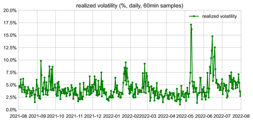
Figure 3: Daily realized volatility for the ETH-USDC pair, computed from Binance minutely closing prices, sampled at 60 minute intervals.

In Figure 4, we see the daily average aggregate value for this pool over the time period. The average pool value was $209 million, and the pool value ranged between $90 million and $310 million.

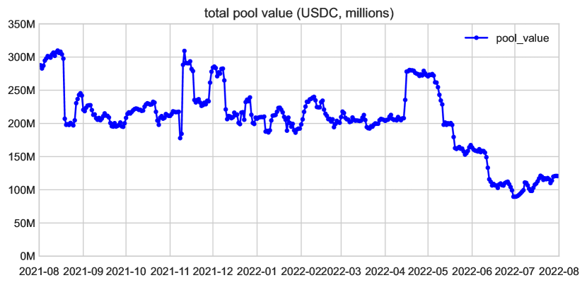
Figure 4: The daily average pool value of the Uniswap v2 WETH-USDC pair.

Next, we show why it is important to account for the profits of the rebalancing strategy in analyzing LP returns. The pool_pnl series in Figure 5(a) shows the raw aggregate LP $\mathsf{P\&L}_{t}$ (i.e., without delta-hedging by subtracting the rebalancing strategy). The pool $\mathsf{P\&L}$ fluctuates wildly, and ultimately loses money. In particular, as shown in Table 1, the pool has an overall annualized return of $-6.20\%$, and a Sharpe ratio of $-0.15$.

However, these returns are largely driven by market risk: at any point in time, the pool maintains half of its value in ETH, and ETH prices varied significantly over this interval. The hedged_pnl series in Figure 5 illustrate hedged $\mathsf{P\&L}$, that is, $\text{LP $\mathsf{P\&L}$}_{t}$ minus the profits of the rebalancing strategy, which is the left side of (17). This hedges directional exposure to ETH prices to first-order, and is just a bet on whether fees are greater than $\mathsf{LVR}$.

Visually, these lines are substantially less volatile than the raw LP $\mathsf{P\&L}_{t}$. This is quantified in Table 1, where we see that a delta-hedged LP position can achieve very low standard deviation of returns and high Sharpe ratios, and that, in general, standard deviations of returns decrease and Sharpe ratios increase with more frequent rebalancing. Moreover, the delta-hedged LP position actually makes positive returns.

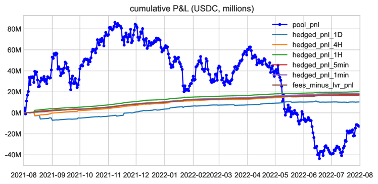
(a) Including the aggregate pool $\mathsf{P\&L}$ series.

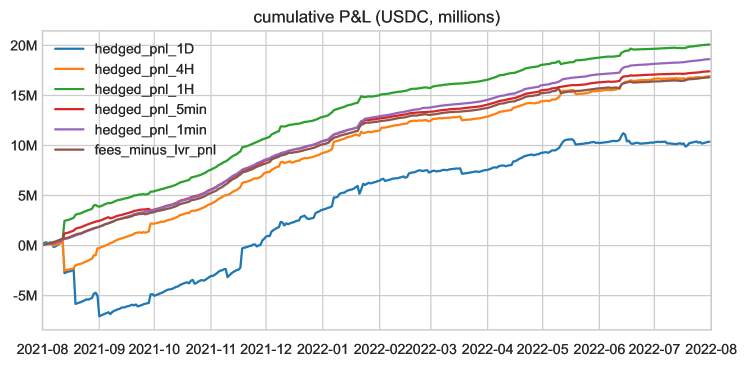
(b) Excluding the aggregate pool $\mathsf{P\&L}$ series.

Figure 5: Cumulative pool $\mathsf{P\&L}$, delta-hedged $\mathsf{P\&L}$, and predicted $\mathsf{P\&L}$ from our expressions for $\mathsf{LVR}$, for the Uniswap v2 WETH-USDC trading pair. In the first panel, the pool_pnl series shows the raw $\mathsf{P\&L}$ of the LP position. In both panels, the various hedged_pnl series show delta-hedged LP $\mathsf{P\&L}$, that is, the $\mathsf{P\&L}$ from a long position in the pool, and a short position in the rebalancing strategy, rebalanced at various frequencies (daily, every four hours, every hour, every five minutes). The fees_minus_lvr_pnl series shows fees minus $\mathsf{LVR}$, this is the delta-hedged $\mathsf{P\&L}$ predicted by our theory. The data source for prices is Binance, and LP $\mathsf{P\&L}$ is calculated using data on Uniswap trades, mints, and burns from the Ethereum blockchain. Details of how we calculate these quantities are in Appendix C.

	avg return	stdev return	Sharpe ratio
	(%, annual)	(%, annual)	(annual)
pool_pnl	-6.20	42.08	-0.15
hedged_pnl_1D	5.04	2.87	1.75
hedged_pnl_4H	8.21	1.50	5.47
hedged_pnl_1H	9.75	0.90	10.81
hedged_pnl_5min	8.45	0.57	18.16
hedged_pnl_1min	9.04	0.39	23.33
fees_minus_lvr_pnl	8.16	0.48	17.03

Table 1: Overall return statistics for the cumulative $\mathsf{P\&L}$ series of Figure 5.

Accuracy of the model. In Figure 6, we analyze the accuracy of our model, that is, the difference between the left and right sides of (17), for various choices of frequency of rebalancing. This analyzes how well our model is able to predict delta-hedged LP returns in the data. Fees minus $\mathsf{LVR}$ in our model tracks the pattern of hedged LP $\mathsf{P\&L}$: differences between the two seem to be stationary over the observed interval. Moreover, in general, as the frequency of rebalancing increases, the differences are smaller in magnitude. This is consistent with $\mathsf{LVR}$ as being a continuous rebalancing approximation.

Using delta-hedged LPing in other contexts. Our procedure is easily generalizable: any researcher interested in analyzing the economic determinants of AMM LP returns can use our ‘‘hedged LPing’’ methodology to eliminate LP positions’ market risk exposures. The procedure has very low data requirements: to construct profits of the rebalancing strategy, (18), the researcher only needs $x_{t}^{RB}$, the time series of risky asset holdings of the CFMM LP, and $P_{t}$, the CEX price of the risky asset. Hedged LP $\mathsf{P\&L}$ is then just the difference between raw pool PNL and the return on the rebalancing strategy.

We believe our methodology is a substantial improvement over existing methods in the literature to remove market risk exposures from LP $\mathsf{P\&L}$. Some papers, such as Fang (2022), use risk factor models to account for the component of LP returns attributable to market risk. Relative Our methodology is much simpler: since a CFMM holds risky assets, it has first-order exposure to risky asset prices at any point in time equal to whatever amount of the risky asset it holds. These risk exposures can be accounted for simply by shorting the risky asset itself: this does not require taking a stance on a risk factor model, and estimating factor loadings.

Other papers, such as Lehar et al. (2022) and Augustin et al. (2022), decompose LP $\mathsf{P\&L}$ by subtracting ‘‘impermanent loss’’ — loss versus a strategy which holds the initial asset position. ‘‘Impermanent loss’’ — which we will refer to as ‘‘loss versus holding’’ or $\mathsf{LVH}$— compares LP performance to a benchmark which simply holds the initial bundle of risky assets. As we discuss in Section 8, this combines losses from price slippage, which are always greater than 0, with the returns from the rebalancing strategy, which can be thought of as a particular trading strategy that bets on mean reversion. Impermanent loss is always equal in expectation to $\mathsf{LVR}$ under risk-neutral measure, but will always be noisier than $\mathsf{LVR}$. Subtracting ‘‘impermanent loss’’ from LP returns thus results in, at best, a much noisier measure of returns, relative to $\mathsf{LVR}$, reducing the likelihood that the researcher can elucidate economic effects with high statistical power.

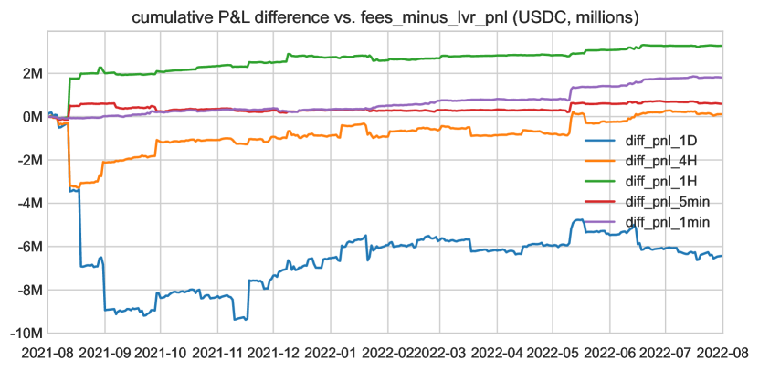
Figure 6: Cumulative differences between the delta-hedged $\mathsf{P\&L}$ (various hedged_pnl series of Figure 5) and predicted $\mathsf{P\&L}$ from our model (fees_minus_lvr_pnl series of Figure 5).

7 Option Pricing

We have shown that CFMM LPs behave like a bet on volatility, in the sense that $\mathsf{LVR}$ is large when volatility is high. In this section, we briefly discuss the relationship of CFMM LPs to three classical and inter-related ways that volatility can be traded (Carr and Madan, 2001): static (European) options positions, dynamic trading strategies, and variance swaps. In Section B.1, we also demonstrate the equivalences between CFMM LP positions and these concepts in a simple two-step binomial tree model.

7.1 Static Options Positions

Our results are related to Clark (2020), Fukasawa et al. (2022), and Deng et al. (2023), who show that, over any finite time horizon, an AMM LP position’s payoff, ignoring fees, can be replicated by shorting a bundle of European options. Technically, this follows from the facts that the CFMM’s asset position and value are both path-independent: if the price is $P_{T}$ at time $T$, the CFMM holds $x^{*}(P_{T})$ of the risky asset and has pool value $V_{T}=V(P_{T})$ corresponding to the final ‘‘payoff function’’ $V(\cdot)$, regardless of the path that prices took to reach $P_{T}$. More intuitively, at any time $T$, the CFMM simply offers a menu of quantities of the asset to buy or sell at any given price, identically to a portfolio of European options. Ignoring fees, the CFMM exactly breaks even if prices do not move, $P_{T}=P_{0}$, and loses money otherwise; hence, the CFMM LP position is essentially equivalent to giving away a bundle of European options. This intuition is consistent with the fact that the $V(\cdot)$ is a concave function (cf. Lemma 1).

Expected $\mathsf{LVR}$ until period $T$ can be thought of as the value of the European options given away. This analogy gives another intuition for the comparative statics of expected $\mathsf{LVR}$. European options are worth more when volatility is higher, so $\mathsf{LVR}$ is increasing in the volatility of the underlying asset. When the marginal liquidity of the AMM bonding curve is greater, the replicating portfolio of European options is larger: AMMs that trade more aggressively essentially give away more European options, also increasing $\mathsf{LVR}$.

As previous papers have discussed, the European option replication result also implies that, over any finite time horizon, the exposure of the AMM LP position to underlying prices can be totally hedged, by taking a long position in the replicating bundle of European options. This trade — a long position in the AMM LP, plus a short position in the replicating bundle of European options — is essentially a trading fee swap, betting on whether accrued trading fees from time $0$ to $T$ are greater than European option premia of the replicating portfolio at time $0$. The trader enters an LP position, and pays a premium for buying the replicating bundle of European options upfront. The AMM LP position then loses no money from price movements; the total position profits if the accrued trading fees until time $T$ are greater than the European option premia paid upfront, and loses otherwise.

7.2 Dynamic Trading Strategies

Classic options theory implies that static option positions are equivalent to dynamically trading the underlying asset in a certain way. The static option position is a combination of short straddles and strangles, selling out-of-money calls and puts. This position is equivalent to a dynamic trading strategy which sells the asset when prices increase, and buys when prices decrease. This is exactly what the AMM LP position does: observe that, from Lemma 1 Part 3, $x^{*}(\cdot)$ is non-increasing. If prices decrease slightly from $P_{0}$ to $P_{t}<P_{0}$, the rebalancing strategy responds by buying the risky asset. The rebalancing strategy thus makes a profit, relative to simply holding the initial position $x^{*}\left(P_{0}\right)$, if prices increase back to $P_{0}$, and makes a loss if prices decrease further from $P_{t}$. This argument holds symmetrically for price decreases, implying that the rebalancing strategy makes losses if prices diverge from $P_{0}$, and profits when prices make small movements away from $P_{0}$ and back. In the special case where the risky asset’s price is a random walk, the rebalancing strategy thus breaks even on on average. In contrast, when prices move away from $P_{0}$ and back, the CFMM reverts to the initial value $V\left(P_{0}\right)$, exactly breaking even: there is no profit from price convergence, to offset the losses the CFMM makes when prices diverge from $P_{0}$.

7.3 Variance Swaps

Finally, as discussed by Fukasawa et al. (2022), variance can be traded directly by trading swaps on realized variance. The VIX is such a contract, operating on a fixed finite time horizon. Applying Lemma 1 Part 3, the instantaneous $\mathsf{LVR}$ of (8) can be re-written as

$$\ell(\sigma,P)=\tfrac{1}{2}\times(\sigma P)^{2}\times|x^{*\prime}(P)|.$$

Here, the first component, $(\sigma P)^{2}$, is the instantaneous variance or quadratic variation of the price, i.e., for small $\Delta t$, $\operatorname{Var}[P_{t+\Delta t}|P_{t}=P]\approx(\sigma P)^{2}\,\Delta t$. Recalling that $x^{*}(P)$ is the total quantity of risky asset held by the pool if the price is $P$, the second component, $|x^{*\prime}(P)|$ corresponds to the marginal liquidity available from the pool at price level $P$. Now, integrating over time, we have that

$$\mathsf{LVR}_{t}=\tfrac{1}{2}\int_{0}^{t}(\sigma_{s}P_{s})^{2}\times|x^{*\prime}(P_{s})|\,ds=\tfrac{1}{2}\int_{0}^{t}|x^{*\prime}(P_{s})|\,d[P]_{s},\quad\forall\ t\geq 0.$$

This expression is the payoff of the floating leg of a continuously sampled generalized variance swap (Carr and Lee, 2009, see, e.g.,), specifically a price variance swap that is weighted by marginal liquidity.

8 Other Benchmarks and ‘‘Impermanent Loss’’

In this section, we consider the possibility of alternative benchmarks aside from the rebalancing strategy. We first define a broad class of benchmark strategies: the only restrictions we impose on these strategies are that they begin holding the same position in the risky asset as the CFMM, and that they adjust holdings at CEX prices. Specifically, we define a benchmark as a self-financing trading strategy, described by a position $\bar{x}_{t}$ in the risky asset. We assume that initial holdings match the pool, i.e., $(\bar{x}_{0},\bar{y}_{0})\triangleq\big{(}x^{*}(P_{0}),y^{*}(P_{0})\big{)}$. We assume that $\bar{x}_{t}$ satisfies the square-integrability condition (3), so that the resulting trading strategy is admissible. Denote the value of that strategy by $\bar{R}_{t}$, so that

$$\bar{R}_{t}=V_{0}+\int_{0}^{t}\bar{x}_{s}\,dP_{s},\quad\forall\ t\geq 0.$$

For any such benchmark, we can thus define the loss-versus-benchmark according to $\mathsf{LVB}_{t}\triangleq\bar{R}_{t}-V_{t}$. The following result characterizes the loss process $\mathsf{LVB}_{t}$ as a function of the underlying benchmark strategy $\bar{x}_{t}$.

Corollary 1.

For all $t\geq 0$,

$$\begin{split}\mathsf{LVB}_{t}&=\mathsf{LVR}_{t}+\underbrace{\int_{0}^{t}\left[\bar{x}_{s}-x^{*}(P_{s})\right]\,dP_{s}}_{\triangleq\Delta(\bar{x})_{t}},\end{split}$$ (20)

and at the same time,

$$\mathsf{E}^{\mathbb{Q}}\left[\mathsf{LVB}_{t}\right]=\mathsf{E}^{\mathbb{Q}}\left[\mathsf{LVR}_{t}\right]\,.$$ (21)

The loss process has quadratic variation

$$[\mathsf{LVB}]_{t}=[\Delta(\bar{x})]_{t}=\int_{0}^{t}\left[\bar{x}_{s}-x^{*}(P_{s})\right]^{2}\,\sigma_{s}^{2}P_{s}^{2}\,ds\geq[\mathsf{LVR}]_{t}=0.$$ (22)

Therefore, among all benchmark strategies, the rebalancing strategy uniquely defines a loss process with minimal (zero) quadratic variation.

Proof.

The first part is an immediate corollary of Theorem 1 and (5). The second part is immediate by the definition of the risk-neutral measure. The third part follows from the Itô isometry. ∎

There are two ways to interpret Corollary 1. On the one hand, in (20), the expected value of $\Delta(\bar{x})_{t}$ is always 0 under the risk-neutral measure. Thus, the second part of Corollary 1 expresses that the risk-neutral expectation of $\mathsf{LVB}$ is the same for any choice of benchmark, including $\mathsf{LVR}$ and the $\mathsf{HODL}$ benchmark. This is because CFMM LP losses arise from trading at off-market prices: any benchmark which trades at market prices, in expectation, does equally well under the risk-neutral measure, and thus the gap between any market benchmark and $\mathsf{LVR}$ is equal in expectation. In this sense, the market price of the expected losses of CFMM LPs is invariant to the particular choice of market-based benchmark.

On the other hand, $\mathsf{LVR}$ is the unique choice of benchmark which eliminates differences in performance between the CFMM and the benchmark strategy due to market risk, and isolating losses due to price slippage. All benchmarks outperform the CFMM LP position by the same amount in expectation; however, on any given price path $P_{t}$, any given benchmark may over- or underperform to the CFMM LP position, because the benchmark may adopt different holding strategies for the risky asset from the CFMM. As an example, we showed in Section 6 that the CFMM LP position underperforms a benchmark which sells all ETH and holds $\bar{x}_{t}=0$ throughout, because of the fact that the CFMM LP holds a larger ETH position and ETH prices dropped over the time horizon we analyze, implying the misleading conclusion that the CFMM LP position underperformed a market-based benchmark.

The $\mathsf{LVR}$ benchmark is useful because the rebalancing strategy exactly matches the risky asset holdings of the CFMM, removing differences in market risk exposure and isolates losses due to slippage. Theorem 1 showed that $\mathsf{LVR}$ is a strictly increasing process: it is always positive, regardless of the path prices take. Expression (22) thus shows that the rebalancing strategy is the unique choice of benchmark which minimizes the quadratic variation of the loss process: that is, any other choice of benchmark can be thought of as $\mathsf{LVR}$, plus a noise term which has mean 0 under risk-neutral measure, caused by differences in market risk exposures. Thus, in our view, benchmarks other than the rebalancing strategy confound two concepts: $\mathsf{LVR}$, which captures losses of the CFMM LP position due to trading at off-market prices, and $\Delta(\bar{x})$, which captures differences between the risky asset holdings of the CFMM and the benchmark.

One benchmark of particular interest is a strategy that simply holds the initial position, i.e., $x_{t}^{\mathsf{HODL}}\triangleq x^{*}(P_{0})$, with value

$$R_{t}^{\mathsf{HODL}}=V_{0}+\int_{0}^{t}x^{*}(P_{0})\,dP_{s}=V_{0}+x^{*}(P_{0})\left(P_{t}-P_{0}\right),\quad\forall\ t\geq 0.$$

Loss versus the $\mathsf{HODL}$ benchmark, introduced by Pintail (2019), is sometimes known by practitioners as ‘‘impermanent loss’’ or ‘‘divergence loss’’ (e.g., Engel and Herlihy, 2021). Motivated by the aforementioned analysis, in our view this is more accurately described as ‘‘loss-versus-holding’’: $\mathsf{LVH}_{t}\triangleq R_{t}^{\mathsf{HODL}}-V_{t}$. Like $\mathsf{LVR}$, $\mathsf{LVH}$ is $\mathsf{LVH}$ is always non-negative:

Proposition 1.

For all $t\geq 0$,

$$\mathsf{LVH}_{t}\geq 0,$$ (23)

i.e., $\mathsf{LVH}$ is a non-negative process.

Proof.

We have that

$$\mathsf{LVH}_{t}=R_{t}^{\mathsf{HODL}}-V_{t}=\left(P_{t}x^{*}(P_{0})+y^{*}(P_{0})\right)-\left(P_{t}x^{*}(P_{t})+y^{*}(P_{t})\right),$$

and, by the optimality of Equation 1 for $P=P_{t}$, this quantity is always non-negative. ∎

While $\mathsf{LVH}$ is non-negative, it cannot be viewed as a true ‘‘running cost’’: $\mathsf{LVH}$, like any $\mathsf{LVB}$ for any non-rebalancing benchmark, contains a market risk component, and it can always revert. Indeed, from (20), the only permanent and non-reverting component of $\mathsf{LVH}$ is $\mathsf{LVR}$. Beyond that, there are other disadvantages to $\mathsf{LVH}$ as a cost metric. First, $\mathsf{LVH}$ depends on the initial position at time $t=0$. This means that two different LPs investing in a pool will realize different $\mathsf{LVH}$ over the same interval of time, depending on the pool holdings at their respective initial times of investment. To contrast, $\mathsf{LVR}$ over the same interval of time is the same (up to proportionality of the investment size) for all LPs. Another disadvantage of $\mathsf{LVH}$ is that it is path independent: the value of $\mathsf{LVH}$ depends only on the asset price at the beginning and end of the observation interval. On the other hand, $\mathsf{LVR}$ is path dependent and depends on the entire sample path. This makes more sense for an adverse selection cost: the profitability of market making should depend on realized volatility or quadratic variation over the time interval, as $\mathsf{LVR}$ does.

A common argument in the industry discourse for the benchmark of ‘‘impermanent loss’’ states that, as long as prices revert to their initial values, AMM holdings will also revert to their initial state, resulting in zero losses. We analyze this argument in Section B.1. In a slight departure from our baseline model, we assume prices evolve according to a two-step binomial tree. In the first step of the tree, the risky asset’s price either increases or decreases; in the second step, prices can either revert to their initial level, or diverge further. The basic trading strategy of an CFMM is to sell the risky asset when its price increases, and buy when its price decreases. Trading in this manner is a bet on mean reversion: when implemented trading at CEX prices, as the rebalancing strategy does, the strategy profits if prices mean-revert, and loses if prices diverge further, thus breaking even on average. The CFMM executes the same trades as the rebalancing strategy, but attains worse prices on each trade. Thus, the CFMM exactly breaks even if prices mean-revert, and loses more money than the rebalancing strategy if prices diverge, thus losing money on average. This example illustrates that, for an CFMM to perform well, it is not sufficient to break even when prices revert; a trading strategy which sells into price rises and buys into price decreases must actually make strictly positive profits when prices revert, in order to compensate for the losses it makes when prices diverge. An AMM’s performance should thus be benchmarked to the rebalancing strategy — making the same trades at CEX prices — rather than the intuitive but misleading benchmark that the CFMM should break even upon price reversion.

9 Discussion and Implications

Besides their positive value for understanding and quantifying the losses from AMM LPing, our results also suggest ways that these losses could be reduced or eliminated. We have shown that $\mathsf{LVR}$ changes based on market conditions: $\mathsf{LVR}$ is greater when volatility is high. This suggests the utilization of dynamic trading fee rules: trading fees could be adjusted based on volatility or variance. These adjustments could in principle be based on the recent past (e.g., historical realized volatility or realized $\mathsf{LVR}$), or on future predictions (e.g., options-implied volatility).

We showed that CFMM LPs lose money from price slippage: when CEX prices move, CFMM quotes become ‘‘stale’’ and are vulnerable to sniping by rebalancing arbitrageurs. It is in principle possible to eliminate this slippage: if an AMM had access to a high-frequency oracle for the CEX price $P_{t}$, the AMM could in principle quote prices arbitrarily close to $P_{t}$, up to the desired asset position $x^{*}\left(P_{t}\right)$. Quoting prices this way would reduce arbitrageurs’ profits, allowing the AMM to achieve a payoff arbitrarily close to that of the rebalancing strategy. This design has a number of risks — it relies heavily on the accuracy of the oracle for $P_{t}$, and leaves open the potential for oracle manipulation — but in principle an oracle-based AMM could substantially reduce or eliminate $\mathsf{LVR}$.

A related set of AMM designs revolve around selling the right to arbitrage the pool to certain special wallets, and redistributing profits to AMM LPs. This could be done in several ways. Suppose a particular crypto wallet address, which we call the ‘‘authorized participant’’ or AP, had the unique right for the first AMM trade in every block. This first execution right effectively conveys the right to arbitrage the pool (Josojo, 2022). Alternatively, the AP could be provided the right to trade with the AMM paying zero fees (Jump Crypto, 2022). The AP would then have a large advantage in arbitrage trading, since the AP could profitably trade against arbitrarily small price movements, whereas prices would have to move at least as much as the AMM’s percentage trading fees for non-AP wallets to profit from arbitrage trade. The AP would thus be able to capture a large fraction of fees from arbitrage trade.

In either of these designs, an AMM protocol aiming to reduce $\mathsf{LVR}$ could thus run an AP wallet itself, doing CEX-DEX arbitrage, and redistributing arbitrage profits to LPs. Alternatively, AMM protocols could simply run periodic auctions — over longer periods, such as weeks or months — in which wallets can bid for the right to be authorized participants for some period of time. In principle, potential arbitrageurs should bid the ex ante expectation of arbitrage profits, which includes $\mathsf{LVR}$; the protocol can then redistribute these profits to LPs. Both these methods capture either $\mathsf{LVR}$ or its expectation, and redistribute the profits to pool LPs. We believe that these are interesting directions for future AMM design research.

10 Conclusion

In this paper, we constructed a model of AMM LP profits. We defined the losses suffered by LPs as ‘‘loss-versus-rebalancing’’, or $\mathsf{LVR}$; this is the gap between the profits of an AMM LP position, and the returns from a trading strategy which perfectly mimics the AMM’s position in the risky asset, but performs all trades at market prices. $\mathsf{LVR}$ arises from the fact that AMMs always trade at off-market prices, leaving money to arbitrageurs trading the AMM against a CEX. $\mathsf{LVR}$ is greater when prices are more volatile, and when the AMM’s ‘‘marginal liquidity’’ is greater, that is, it trades more aggressively in response to price movements. A delta-hedged AMM LP position — a position which is long the LP position, and short the rebalancing strategy — is profitable if the AMM collects more in fees than it loses in $\mathsf{LVR}$. The model is quantitatively realistic enough to be brought to data; we show that our expressions for $\mathsf{LVR}$ predict AMM LP losses fairly accurately in practice. Our results have implications for how to redesign AMMs to reduce or eliminate $\mathsf{LVR}$, which could lower the effective trading fees paid by market participants relying on AMMs for token pair liquidity.

Appendix A Proofs

A.1 Proof of Theorem 1

First, we show that $\mathsf{LVR}_{t}$ is equal to expression (7). The smoothness condition of Assumption 1 Part 2 allows us to apply Itô’s lemma to $V(\cdot)$ to obtain

$$\begin{split}dV_{t}&=V^{\prime}(P_{t})\,dP_{t}+\tfrac{1}{2}V^{\prime\prime}(P_{t})\left(dP_{t}\right)^{2}\\ &=V^{\prime}(P_{t})\,dP_{t}+\tfrac{1}{2}V^{\prime\prime}(P_{t})\,\sigma^{2}P_{t}^{2}\,dt\\ &=x^{*}(P_{t})\,dP_{t}+\tfrac{1}{2}V^{\prime\prime}(P_{t})\,\sigma^{2}P_{t}^{2}\,dt,\end{split}$$ (24)

where the last step follows from Lemma 1 Part 2. Comparing with (5), we obtain (7). Finally, the fact that $\ell(\sigma,P)\geq 0$ follows from Lemma 1 Part 3.

Next, we show that the cumulative profits of rebalancing arbitrageurs is equal to $\mathsf{LVR}_{t}$. We start with a discrete approximation to the arbitrage profit, indexed by $N\geq 1$. Suppose arbitrageurs arrive sequentially, so that the $i$th arbitrageur arrives at time $\tau_{i}$, for $1\leq i\leq N$. For convenience, set $\tau_{0}\triangleq 0$ and $\tau_{N+1}\triangleq T$. For each $1\leq i\leq N$, at time $\tau_{i}$, the $i$th arbitrageur observes the price $P_{\tau_{i}}$, rebalances the pool from $\big{(}x^{*}(P_{\tau_{i-1}}),y^{*}(P_{\tau_{i-1}})\big{)}$ to $\big{(}x^{*}(P_{\tau_{i}}),y^{*}(P_{\tau_{i}})\big{)}$. In other words, the arbitrageur purchases $x^{*}(P_{\tau_{i-1}})-x^{*}(P_{\tau_{i}})$ units of the risky asset from the CFMM at average price :

$$P_{i}^{\mathsf{CFMM}}\triangleq-\frac{y^{*}(P_{\tau_{i}})-y^{*}(P_{\tau_{i-1}})}{x^{*}(P_{\tau_{i}})-x^{*}(P_{\tau_{i-1}})}.$$

The arbitrageur can then sell these units on the external market at price $P_{\tau_{i}}$ and earn profits (in the numéraire) from the difference in price according to

$$\left(P_{\tau_{i}}-P_{i}^{\mathsf{CFMM}}\right)\left[x^{*}(P_{\tau_{i-1}})-x^{*}(P_{\tau_{i}})\right]=P_{\tau_{i}}\left[x^{*}(P_{\tau_{i-1}})-x^{*}(P_{\tau_{i}})\right]+\left[y^{*}(P_{\tau_{i-1}})-y^{*}(P_{\tau_{i}})\right].$$

Denote by $\mathsf{ARB}_{T}^{(N)}$ the aggregate arbitrage profits. Summing over $1\leq i\leq N$, telescoping the sum, and applying summation-by-parts yields

$$\begin{split}\mathsf{ARB}_{T}^{(N)}&\triangleq\sum_{i=1}^{N}\left\{P_{\tau_{i}}\left[x^{*}(P_{\tau_{i-1}})-x^{*}(P_{\tau_{i}})\right]+\left[y^{*}(P_{\tau_{i-1}})-y^{*}(P_{\tau_{i}})\right]\right\}\\ &=\sum_{i=1}^{N}P_{\tau_{i}}\left[x^{*}(P_{\tau_{i-1}})-x^{*}(P_{\tau_{i}})\right]+y^{*}(P_{0})-y^{*}(P_{\tau_{N}})\\ &=P_{0}x^{*}(P_{0})+y^{*}(P_{0})+\sum_{i=0}^{N}x^{*}(P_{\tau_{i}})\left[P_{\tau_{i+1}}-P_{\tau_{i}}\right]-P_{T}x^{*}(P_{\tau_{N}})-y^{*}(P_{\tau_{N}}).\end{split}$$

Observe that the sum in the final expression is the discrete approximation of an Itô integral. Assume that the time partition mesh over $[0,T]$ shrinks to zero as $N\rightarrow\infty$. Taking the limit as $N\rightarrow\infty$ and passing to continuous time, the sum converges to an Itô integral, which is well-defined under Assumption 1 Part 3. Further, $\tau_{N}\rightarrow T$, so that $P_{\tau_{N}}\rightarrow P_{T}$, and $x^{*}(P_{\tau_{N}})\rightarrow x^{*}(P_{T})$, $y^{*}(P_{\tau_{N}})\rightarrow y^{*}(P_{T})$. Thus, it holds that

$$\mathsf{ARB}_{T}\triangleq\lim_{N\rightarrow\infty}\mathsf{ARB}_{T}^{(N)}=V(P_{0})+\int_{0}^{T}x^{*}(P_{t})\,dP_{t}-V(P_{T}).$$

Hence, the cumulative profits of rebalancing arbitrageurs from time $0$ to time $T$ are equal to $\mathsf{LVR}$, defined in (6).

A.2 LVR, Marginal Liquidity, and Bonding Function Curvature

For sufficiently smooth CFMM bonding functions, the marginal liquidity can be expressed in terms of derivatives of the CFMM bonding function:

$$\frac{dx}{dP}=\frac{\frac{\partial f}{\partial y}}{\left(\frac{\partial^{2}f}{\partial x^{2}}+P^{2}\frac{\partial^{2}f}{\partial y^{2}}-2P\frac{\partial^{2}f}{\partial x\partial y}\right)}$$ (25)

Qualitatively, (25) implies that marginal liquidity, $x^{\prime}\left(P\right)$, is related to the curvature of the CFMM invariant curves. The denominator of (25) is equal to $P^{2}$ times the negative of the determinant of the bordered Hessian of $f$. $f$ is strictly quasiconcave — that is, the upper level sets of $f$ are convex — if and only if this determinant is positive; moreover, the magnitude of the determinant is related to the curvature of the level curves of $f$ (Simon et al., 1994, p. 542). Thus, CFMM invariants with ‘‘flatter’’, more linear level curves will have greater marginal liquidity $\frac{dx}{dP}$, and also greater $\mathsf{LVR}$.

(25) is also useful because it can be used to calculate $\frac{dx}{dP}$ using analytic expressions for bonding functions, which may be useful for computing $\mathsf{LVR}$ in practice.

A.2.1 Derivation of (25)

The Lagrangian of the pool expenditure minimization problem, (1), is:

$$\Lambda=Px+y+\lambda\left[f\left(x,y\right)-L\right]$$

The optimal solution is characterized by the FOCs:

$$\frac{\partial\Lambda}{\partial x}:\ P+\lambda\frac{\partial f}{\partial x}=0$$ (26)

$$\frac{\partial\Lambda}{\partial y}:\ 1+\lambda\frac{\partial f}{\partial y}=0$$ (27)

$$\frac{\partial\Lambda}{\partial\lambda}:\ f\left(x,y\right)-L=0$$ (28)

Now, we will take $\frac{dx}{dP}$ by applying the implicit function theorem to this system of first-order conditions. The derivatives of the FOCs are:

$$\frac{\partial}{\partial P}\frac{\partial\Lambda}{\partial x}:\ 1$$

$$\frac{\partial}{\partial P}\frac{\partial\Lambda}{\partial y}:\ 0$$

$$\frac{\partial}{\partial P}\frac{\partial\Lambda}{\partial\lambda}:\ 0$$

$$\frac{\partial}{\partial x}\frac{\partial\Lambda}{\partial x}:\ \lambda\frac{\partial^{2}f}{\partial x^{2}}$$

$$\frac{\partial}{\partial x}\frac{\partial\Lambda}{\partial y}:\ \lambda\frac{\partial^{2}f}{\partial x\partial y}$$

$$\frac{\partial}{\partial x}\frac{\partial\Lambda}{\partial\lambda}:\ \frac{\partial f}{\partial x}$$

$$\frac{\partial}{\partial y}\frac{\partial\Lambda}{\partial x}:\ \lambda\frac{\partial^{2}f}{\partial x\partial y}$$

$$\frac{\partial}{\partial y}\frac{\partial\Lambda}{\partial y}:\ \lambda\frac{\partial^{2}f}{\partial y^{2}}$$

$$\frac{\partial}{\partial y}\frac{\partial\Lambda}{\partial\lambda}:\ \frac{\partial f}{\partial y}$$

$$\frac{\partial}{\partial\lambda}\frac{\partial\Lambda}{\partial x}:\ -\frac{\partial f}{\partial x}$$

$$\frac{\partial}{\partial\lambda}\frac{\partial\Lambda}{\partial y}:\ -\frac{\partial f}{\partial y}$$

$$\frac{\partial}{\partial\lambda}\frac{\partial\Lambda}{\partial\lambda}:\ 0$$

Hence, we wish to solve the following system of equations for $\frac{dx}{dP}$:

$$\frac{\partial}{\partial P}\frac{\partial\Lambda}{\partial x}+\frac{\partial}{\partial x}\frac{\partial\Lambda}{\partial x}\frac{dx}{dP}+\frac{\partial}{\partial y}\frac{\partial\Lambda}{\partial x}\frac{dy}{dP}+\frac{\partial}{\partial\lambda}\frac{\partial\Lambda}{\partial x}\frac{d\lambda}{dP}=0$$

$$\frac{\partial}{\partial P}\frac{\partial\Lambda}{\partial y}+\frac{\partial}{\partial x}\frac{\partial\Lambda}{\partial y}\frac{dx}{dP}+\frac{\partial}{\partial y}\frac{\partial\Lambda}{\partial y}\frac{dy}{dP}+\frac{\partial}{\partial\lambda}\frac{\partial\Lambda}{\partial y}\frac{d\lambda}{dP}=0$$

$$\frac{\partial}{\partial P}\frac{\partial\Lambda}{\partial\lambda}+\frac{\partial}{\partial x}\frac{\partial\Lambda}{\partial\lambda}\frac{dx}{dP}+\frac{\partial}{\partial y}\frac{\partial\Lambda}{\partial\lambda}\frac{dy}{dP}+\frac{\partial}{\partial\lambda}\frac{\partial\Lambda}{\partial\lambda}\frac{d\lambda}{dP}=0$$

Substituting, we have:

$$1+\lambda\frac{\partial^{2}f}{\partial x^{2}}\frac{dx}{dP}+\lambda\frac{\partial^{2}f}{\partial x\partial y}\frac{dy}{dP}-\frac{\partial f}{\partial x}\frac{d\lambda}{dP}=0$$ (29)

$$0+\lambda\frac{\partial^{2}f}{\partial x\partial y}\frac{dx}{dP}+\lambda\frac{\partial^{2}f}{\partial y^{2}}\frac{dy}{dP}-\frac{\partial f}{\partial y}\frac{d\lambda}{dP}=0$$ (30)

$$\frac{\partial f}{\partial x}\frac{dx}{dP}+\frac{\partial f}{\partial y}\frac{dy}{dP}=0$$ (31)

Now, applying (26) and (27), we have:

$$\frac{\partial f}{\partial x}=P\frac{\partial f}{\partial y}$$ (32)

Thus, we can simplify (31) to:

$$\frac{dy}{dP}=-P\frac{dx}{dP}$$

Substituting into (29) and (30), we have:

$$1+\lambda\frac{\partial^{2}f}{\partial x^{2}}\frac{dx}{dP}+\lambda\frac{\partial^{2}f}{\partial x\partial y}\left(-P\frac{dx}{dP}\right)-\frac{\partial f}{\partial x}\frac{d\lambda}{dP}=0$$

$$0+\lambda\frac{\partial^{2}f}{\partial x\partial y}\frac{dx}{dP}+\lambda\frac{\partial^{2}f}{\partial y^{2}}\left(-P\frac{dx}{dP}\right)-\frac{\partial f}{\partial y}\frac{d\lambda}{dP}=0$$

Rearranging,

$$\left(\frac{\partial^{2}f}{\partial x^{2}}-P\frac{\partial^{2}f}{\partial x\partial y}\right)\lambda\frac{dx}{dP}=\frac{\partial f}{\partial x}\frac{d\lambda}{dP}-1$$ (33)

$$\left(\frac{\partial^{2}f}{\partial x\partial y}-P\frac{\partial^{2}f}{\partial y^{2}}\right)\lambda\frac{dx}{dP}=\frac{\partial f}{\partial y}\frac{d\lambda}{dP}$$ (34)

Now, multiply (34) by $P$, applying (32), and subtract (33), to get:

$$\left(\frac{\partial^{2}f}{\partial x^{2}}+P^{2}\frac{\partial^{2}f}{\partial y^{2}}-2P\frac{\partial^{2}f}{\partial x\partial y}\right)\lambda\frac{dx}{dp}=-1$$

Now,

$$\frac{dx}{dP}=\frac{-1}{\lambda\left(\frac{\partial^{2}f}{\partial x^{2}}+P^{2}\frac{\partial^{2}f}{\partial y^{2}}-2P\frac{\partial^{2}f}{\partial x\partial y}\right)}$$

Now, to solve for $\lambda$, we simply use (27). Hence, we have:

$$\frac{dx}{dP}=\frac{\frac{\partial f}{\partial y}}{\left(\frac{\partial^{2}f}{\partial x^{2}}+P^{2}\frac{\partial^{2}f}{\partial y^{2}}-2P\frac{\partial^{2}f}{\partial x\partial y}\right)}$$ (35)

This is (25).

Appendix B Other Results

B.1 LVR and Impermanent Loss in a Two-Step Binomial Tree

In this appendix, we consider the performance of the CFMM and the rebalancing strategy, as well as the simple buy-and-hold benchmark, on a two-step binomial tree. This discrete-time model is a departure from our baseline model, but usefully illustrates the intuitions behind how the rebalancing strategy behaves relative to the buy-and-hold strategy, why the CFMM strategy under-performs the rebalancing strategy, and why the benchmark behind the ‘‘impermanent loss’’ concept — that the CFMM should not lose money if prices revert to their original state — is inappropriate.

The binomial tree is a two-period discrete-time model, where prices can either go up or down in each time period. The tree is depicted in Panel A of Figure 7. The price begins at $P_{0}=1$. In the first step of the tree, the price can then increase to $P_{1}^{U}=1.4$, or decrease to $P_{1}^{D}=0.6$. In the second step, from $P_{1}^{U}$, the price can increase to $P_{2}^{UU}=1.8$, or decrease to the original level $P_{1}^{UD}=1$. From $P_{1}^{D}$, the price can increase to the original level $P_{2}^{DU}=1$, or decrease further to $P_{2}^{DD}=0.4$. Note that the tree is set up so that, assuming 0 interest rates, the risk-neutral probabilities of up and down movements are all 0.5 — in other words, prices are martingales if the probabilities of up and down movements are equal, so no strategy trading at market prices should be able to make or lose money in expectation.

We then calculate the asset positions and profits of three strategies in each tree state: the buy-and-hold strategy, which simply holds the initial endowment $\left(x_{0},y_{0}\right)=1,1$ forever; the CFMM; and the rebalancing strategy. To calculate these quantities, for the CFMM, we simply compute what $\left(x_{t},y_{t}\right)$ is as a function of the tree price and the initial state $\left(x_{0},y_{0}\right)$. For the rebalancing strategy, in each tree state, if the CFMM trades from $\left(x_{t},y_{t}\right)$ to $\left(x_{t+1},y_{t+1}\right)$, we assume the rebalancing strategy trades to $x_{t+1}$ at the price $P_{t+1}$; hence, the rebalancing strategy’s cash position is:

$$y_{t+1}=y_{t}-P_{t}\left(x_{t+1}-x_{t}\right)$$

The results are shown in Figure 7. Panel B considers the profits of the buy-and-hold strategy, which simply holds the initial endowment $\left(x_{0},y_{0}\right)=1,1$ forever. This strategy is exposed to market risk, making mark-to-market profits if prices rise and losing if prices fall.

Panel C shows the performance of the rebalancing strategy. Since this strategy trades at market prices, it does not make or lose money in expectation under the risk-neutral measure. In period 1, the rebalancing strategy has exactly the same profits as the buy-and-hold strategy in each state. However, the rebalancing strategy sells the risky asset when prices increase to $P_{1}^{U}=1.4$. This is essentially a bet that prices will decrease; indeed, if prices decrease to $P_{2}^{UD}=1$, the rebalancing strategy makes $2.062$ in profits, which is slightly higher than the buy-and-hold’s profit of $2.000$. Conversely, if prices increase further to $P_{2}^{UU}=1.8$, the rebalancing strategy makes $2.738$, slightly lower than the buy-and-hold strategy’s return of $2.800$. On average, the rebalancing strategy makes $2.400$ conditional on reaching $P_{1}^{U}$, like the buy-and-hold strategy, or any other strategy trading at market prices.

Analogously, if prices first decrease to $P_{1}^{D}=0.6$, the rebalancing strategy buys the risky asset; it profits relative to buy-and-hold when prices increase to $P_{2}^{DU}=1$, and loses if prices decrease further to $P_{2}^{DD}=0.2$. This example shows that the rebalancing strategy is essentially a bet on price convergence. The rebalancing strategy sells into price increases and buys into price decreases; this pays off if prices mean-revert, and loses money if prices diverge further. However, the rebalancing strategy does not make or lose money on average.

The performance of the CFMM is shown in Panel D. The CFMM makes the same trades as the rebalancing strategy; thus, $x_{t}$ is the same in each tree state in panels $C$ and $D$. However, the CFMM always trades at worse-than-market prices; as a result, $y_{t}$ is higher state-by-state on the rebalancing strategy compared to the CFMM. A natural definition of loss-versus-rebalancing in discrete time would be the gap between the CFMM’s $y_{t}$-position, and the rebalancing strategy’s $y_{t}$-position, in each state.

Note that the CFMM strategy has the elegant feature that, if prices revert to $1$ — as in states $P_{2}^{UD}$ and $P_{2}^{DU}$ — the CFMM always holds exactly the same position as the buy-and-hold strategy. This is the basis of the colloquially popular idea that CFMM losses are ‘‘impermanent’’. However, the CFMM loses money in expectation: the average profit of the CFMM, across states, is lower than the buy-and-hold strategy in both periods 1 and 2. Essentially, the CFMM bets on convergence, like the rebalancing strategy, but does so in a very inefficient way. The CFMM exactly breaks even if prices revert to their initial state, and loses money — even relative to the rebalancing strategy — if prices diverge. The CFMM strategy thus cannot break even without fees, because there is no state of the world where the CFMM strategy makes positive amounts. Using the options analogy, an CFMM LP position is a dynamic trading strategy which performs like giving away a straddle without collecting premia: the position loses money whenever prices move, and exactly breaks even when prices end where they started.

This example also shows that the gap between the simple CFMM strategy and the buy-and-hold strategy can be decomposed into two distinct components: the performance of the rebalancing strategy relative to buy-and-hold, and the performance of the CFMM relative to the rebalancing strategy. The gap between the rebalancing strategy and buy-and-hold is a bet on convergence: the rebalancing strategy makes money if prices converge, and loses if prices diverge. The gap between the CFMM and the rebalancing strategy, which is the discrete-time version of $\mathsf{LVR}$, is a systematic loss from slippage which accrues whenever prices move.

Relationships to option strategies. The binomial tree example also helps illustrate the analogy between CFMM LP payoffs and European options The time-2 difference between the payoffs of the rebalancing strategy and the buy-and-hold strategy is positive when prices mean-revert, and negative when prices diverge. Hence, payoffs are similar to those of a short European straddle or strangle position, which involves selling calls and puts which expire after two periods. The positive payoff when prices revert can be thought of as the option premia collected from selling the straddle, and the negative payoffs when prices diverge can be thought of as the payouts to the option buyer, which are made if either the call or the put sold expire in-the-money. The CFMM LP position has a similar pattern of payoffs, but makes 0 profits if prices end where they started. An CFMM LP position, ignoring fees, can thus be thought of like giving away a straddle position, without collecting any upfront option premia. Viewed this way, the equivalence between the rebalancing strategy and the static European strangle on the binomial tree reflects the classic idea that static option positions can be replicated by dynamically trading the underlying asset; in this case, European straddles and strangles are replicated by a strategy which sells the risky asset when prices increase and buys when prices decrease.

Panel A: Binomial Tree

for tree=grow’=east,l sep=4em,s sep=3em,inner sep=2pt [$P_{0}=1.0$, align = center, base = bottom [$P^{U}_{1}=1.4$ [$P^{UU}_{2}=1.8$] [$P^{UD}_{2}=1.0$] ] [$P^{D}_{1}=0.6$ [$P^{DU}_{2}=1.0$] [$P^{DD}_{2}=0.2$] ] ]

Panel B: Buy and Hold Strategy

for tree=grow’=east,l sep=0.8em,s sep=0.8em,inner sep=0.8pt [$\Pi_{t}=2.000$
$(x_{t},y_{t})=(1.000,1.000)$, align = center, base = bottom [$\Pi_{t}=2.400$
$(x_{t},y_{t})=(1.000,1.000)$, align = center, base = bottom [$\Pi_{t}=2.800$
$(x_{t},y_{t})=(1.000,1.000)$, align = center, base = bottom] [$\Pi_{t}=2.000$
$(x_{t},y_{t})=(1.000,1.000)$, align = center, base = bottom] ] [$\Pi_{t}=1.600$
$(x_{t},y_{t})=(1.000,1.000)$, align = center, base = bottom [$\Pi_{t}=2.000$
$(x_{t},y_{t})=(1.000,1.000)$, align = center, base = bottom] [$\Pi_{t}=1.200$
$(x_{t},y_{t})=(1.000,1.000)$, align = center, base = bottom] ] ]

Panel C: Rebalancing Strategy

for tree=grow’=east,l sep=0.8em,s sep=0.8em,inner sep=0.8pt [$\Pi_{t}=2.000$
$(x_{t},y_{t})=(1.00,1.00)$, align = center, base = bottom [$\Pi_{t}=2.400$
$(x_{t},y_{t})=(0.845,1.217)$, align = center, base = bottom [$\Pi_{t}=2.738$
$(x_{t},y_{t})=(0.756,1.378)$, align = center, base = bottom] [$\Pi_{t}=2.062$
$(x_{t},y_{t})=(1.014,1.048)$, align = center, base = bottom] ] [$\Pi_{t}=1.600$
$(x_{t},y_{t})=(1.291,0.825)$, align = center, base = bottom [$\Pi_{t}=2.116$
$(x_{t},y_{t})=(1.032,1.084)$, align = center, base = bottom] [$\Pi_{t}=1.084$
$(x_{t},y_{t})=(2.308,0.622)$, align = center, base = bottom] ] ]

Panel D: CFMM LP

for tree=grow’=east,l sep=0.8em,s sep=0.8em,inner sep=0.8pt [$\Pi_{t}=2.000$
$(x_{t},y_{t})=(1,1)$, align = center, base = bottom [$\Pi_{t}=2.366$
$(x_{t},y_{t})=(0.845,1.183)$, align = center, base = bottom [$\Pi_{t}=2.683$
$(x_{t},y_{t})=(0.745,1.341)$, align = center, base = bottom] [$\Pi_{t}=2.000$
$(x_{t},y_{t})=(1.00,1.00)$, align = center, base = bottom] ] [$\Pi_{t}=1.549$
$(x_{t},y_{t})=(1.291,0.775)$, align = center, base = bottom [$\Pi_{t}=2.000$
$(x_{t},y_{t})=(1.00,1.00)$, align = center, base = bottom] [$\Pi_{t}=0.894$
$(x_{t},y_{t})=(2.236,0.447)$, align = center, base = bottom] ] ]

Figure 7: The performance of buy-and-hold, a constant-product CFMM, and the rebalancing strategy, on a two-step binomial tree. Panel A depicts the binomial tree. The performance of the buy-and-hold strategy is shown in Panel B; the rebalancing strategy is shown in panel C, and the constant product CFMM is shown in panel D. In each panel, $x_{t},y_{t}$ are the holdings of the strategy, and $\Pi_{t}$ is the pool value, $y_{t}+P_{t}x_{t}$.

B.2 Weighted Geometric Mean Market Makers

Weighted geometric mean market makers have the special property that the instantaneous $\mathsf{LVR}$ per dollar of pool value, i.e., $\ell(\sigma,P)/V(P)$, is a constant. The following theorem establishes that these are essentially the only CFMMs for which this is true:

Theorem 2.

Suppose a CFMM satisfies

$$\frac{\ell(\sigma,P)}{V(P)}=c(\sigma),\quad\forall\ P\geq 0.$$ (36)

Then, we have

$$V(P)=L_{1}P^{\theta(\sigma)}+L_{2}P^{1-\theta(\sigma)},$$ (37)

for free constants $L_{1},L_{2}\geq 0$, where

$$\theta(\sigma)\triangleq\frac{1-\sqrt{1-8c(\sigma)/\sigma^{2}}}{2}\leq\frac{1}{2}.$$

Comparing with Example 2, observe that (37) states that is the pool can only be the ‘‘sum’’ of $\theta$ and $1-\theta$ weighted geometric mean market makers. The two degrees of freedom are intuitive, since $\theta$ and $1-\theta$ are exchangeable in (15).

Proof of Theorem 2.

We construct the following ODE from the (36) along with (8),

$$P^{2}V^{\prime\prime}(P)+\bar{c}V(P)=0,$$

with constant $\bar{c}\triangleq 2c/\sigma^{2}$. Make the substitution $P=e^{z}$, to arrive at the equivalent ODE,

$$V^{\prime\prime}(z)-V^{\prime}(z)+\bar{c}V(z)=0,$$

which when solved, along with the known limit condition from (1) that $V(z)\rightarrow 0$ as $z\to-\infty$, by the usual method of linear ODEs results in the generic solution,

$$V(P)=L_{1}P^{\frac{1-\sqrt{1-4\bar{c}}}{2}}+L_{2}P^{\frac{1+\sqrt{1-4\bar{c}}}{2}}=L_{1}P^{\theta}+L_{2}P^{1-\theta}.$$

Note that the above calculation is allowed because the quantity under the root is necessarily non-negative, as if it were not, then $V(P)$ would not be everywhere concave, which must be the case by Lemma 1. ∎

B.3 Multi-Dimensional Generalization

In this section, we describe the multi-dimensional generalization of our results. Specifically, denote by vectors $x\in\mathbb{R}^{n}_{+}$ the reserves in $n\geq 2$ assets (none of which need be the numéraire), and $P_{t}\in\mathbb{R}^{n}_{+}$ a vector of prices (in terms of the numéraire). We assume that the price vector evolves according to geometric Brownian motion, i.e.,

$$dP_{t}=\operatorname{diag}(P_{t})\Sigma_{t}^{1/2}\,dB_{t}^{\mathbb{Q}},\quad\forall\ t\geq 0,$$

with covariance matrix of returns $\Sigma_{t}\in\mathbb{R}^{n\times n}$, $\Sigma_{t}\succeq 0$, and where $B_{t}^{\mathbb{Q}}$ is a standard $\mathbb{Q}$-Brownian motion on $\mathbb{R}^{n}$.

Given a bonding function $f\colon\mathbb{R}^{n}_{+}\rightarrow\mathbb{R}$, define the pool value function $V\colon\mathbb{R}^{n}_{+}\rightarrow\mathbb{R}_{+}$ according to

$$\begin{array}[]{lll}V(P)\triangleq&\mathop{\mathrm{minimize}}\limits_{x\in\mathbb{R}^{n}_{+}}&P^{\top}x\\ &\text{\rm subject to}&f(x)=L.\end{array}$$

Analogous to Assumption 1, we will assume that an optimal solution $x^{*}(P)$ exists for all $P\in\mathbb{R}^{n}_{+}$, that $V(\cdot)$ is twice continuously differentiable, and a suitable square-integrability condition on $x^{*}(\cdot)$.

Analogous to Lemma 1, we have

Lemma 2.

For all prices $P\in\mathbb{R}^{n}_{+}$, the pool value function satisfies:

1. $V(P)\geq 0$.

2. $\nabla V(P)=x^{*}(P)\geq 0$.

3. $\nabla^{2}V(P)=\nabla x^{*}(P)\preceq 0$.

Define the rebalancing strategy by $x_{t}=x^{*}(P_{t})$, with value

$$R_{t}=V_{0}+\int_{0}^{t}x^{*}(P_{s})^{\top}dP_{s},\quad\forall\ t\geq 0.$$

Then, we have the following multi-dimensional analog of Theorem 1:

Theorem 3.

Loss-versus-rebalancing takes the form

$$\mathsf{LVR}_{t}=\int_{0}^{t}\ell(\Sigma_{s},P_{s})\,ds,\quad\forall\ t\geq 0,$$

where we define, for $P\geq 0$, the instantaneous $\mathsf{LVR}$

$$\ell(\Sigma,P)\triangleq-\tfrac{1}{2}\operatorname{tr}\left[\operatorname{diag}(P)\Sigma\operatorname{diag}(P)\,\nabla x^{*}(P)\right]\geq 0,$$

where we have applied Lemma 2. In the case where $\Sigma=\sigma^{2}I$, i.e., i.i.d. assets, we have that

$$\ell(\Sigma,P)=-\frac{\sigma^{2}}{2}\operatorname{tr}\left[\operatorname{diag}(P)^{2}\,\nabla x^{*}(P)\right]=-\frac{\sigma^{2}}{2}\ \sum_{i=1}^{n}\ P_{i}^{2}\frac{\partial}{\partial P_{i}}x^{*}(P)\geq 0.$$

In particular, $\mathsf{LVR}$ is a non-negative, non-decreasing, and predictable process.

Proof.

Applying Itô’s lemma to $V_{t}=V(P)$,

$$\begin{split}dV_{t}&=\nabla V(P_{t})^{\top}\,dP_{t}+\tfrac{1}{2}(dP_{t})^{\top}\nabla^{2}V(P_{t})\,dP_{t}\\ &=x^{*}(P_{t})^{\top}\,dP_{t}+\tfrac{1}{2}\operatorname{tr}\left[\Sigma_{t}^{1/2}\operatorname{diag}(P)\nabla^{2}V(P_{t})\operatorname{diag}(P)\Sigma_{t}^{1/2}\right]\,dt\\ &=dR_{t}-\ell(\Sigma_{t},P_{t})\,dt.\end{split}$$

The rest of the result follows as in the proof of Theorem 1. ∎

Appendix C Data and Measurement

C.1 Data

Prices. We download minute-level USDC-ETH prices from the Binance API. We use close prices at the end of each minute for $P_{t}$.

Uniswap. We download data on the Uniswap v2 WETH-USDC pool from Dune Analytics, a data provider which aggregates data from the Ethereum blockchain into SQL databases. The queries we use to extract this data are included in Section C.2.

Mints and burns. In each minute, we observe the gross amounts of each asset in which are withdrawn through ‘‘burns’’, and deposited through ‘‘mints’’. Let $(x_{t}^{\text{mint}},y_{t}^{\text{mint}})$ and $(x_{t}^{\text{burn}},y_{t}^{\text{burn}})$ be the total amounts of each asset $x$ and $y$ which are minted and burned respectively, between time $t-1$ and time $t$. We will value minted and burned assets at the time-$t$ closing price $P_{t}$. Thus, the monetary value of mints and burns respectively are:

$$\Pi_{t}^{\text{mint}}\triangleq y_{t}^{\text{mint}}+P_{t}x_{t}^{\text{mint}},\quad\Pi_{t}^{\text{burn}}\triangleq y_{t}^{\text{burn}}+P_{t}x_{t}^{\text{burn}}.$$

Let $(x_{t},y_{t})$ be the total asset holdings of the pool at time $t$. As in the model, define the pool value at time $t$ by

$$V_{t}\triangleq y_{t}+P_{t}x_{t}.$$

We can calculate $\Delta\text{LP\ $\mathsf{P\&L}_{t}$}$, the change in $\mathsf{P\&L}$ of the pool, from period $t-1$ to $t$, as

$$\Delta\text{LP\ $\mathsf{P\&L}_{t}$}\triangleq V_{t}+\Pi_{t}^{\text{burn}}-\Pi_{t}^{\text{mint}}-V_{t-1}.$$ (38)

In words, this is the value of pool reserves at time $t$ valued at price $P_{t}$, plus burned assets and minus minted assets valued at $P_{t}$, minus the value of pool reserves at time $t-1$ valued at $P_{t-1}$. Note that, in contrast to our simplifying assumption in the model that fees are paid in the numéraire, in practice in Uniswap v2 fees are paid directly into the pool reserves; hence, the pool $\mathsf{P\&L}$ includes transaction fees paid into the pool.

Rebalancing strategy. We rebalance the pool at different time frequencies. For each rebalancing frequency, we compute the returns of a strategy which at any point in time holds as much ETH as the pool holds at the start of the period. For example, if the rebalancing frequency is daily, we set $x_{t}^{RB}$ at any minute $t$ equal to the LP pool reserves at the start of the day containing the minute $t$. We then calculate the returns on the rebalancing strategy using expression (18), that is:

$$\Delta\text{RB\ $\mathsf{P\&L}_{t}$}=x_{t}^{RB}\left(P_{t+1}-P_{t}\right).$$ (39)

Fees. In each minute, we compute the gross amount of each asset in the pair bought and sold. The Uniswap v2 pool has a fixed fee rate of 30bps on the contributed asset; we thus calculate fees in each asset by multiplying the gross amount contributed of each asset by 0.003. Call these fees $x_{t}^{fee}$ and $y_{t}^{fee}$ in period $t$. We value fees at the period $t$ price; thus, the monetary value of fees in period $t$, which we will call $\Delta\mathsf{FEE}_{t}$, is:

$$\Delta\mathsf{FEE}_{t}\triangleq y_{t}^{fee}+P_{t}x_{t}^{fee}.$$ (40)

LVR. We compute a realized daily volatility using USDC-ETH prices from the Binance API sampled at 60 minute intervals. Let $\Delta\mathsf{LVR}_{t}$ be the increment of $\mathsf{LVR}$ in period $t$. As in Example 3, we then calculate $\Delta\mathsf{LVR}_{t}$ simply as

$$\Delta\mathsf{LVR}_{t}\triangleq\frac{\hat{\sigma}^{2}_{t}}{8}\times V_{t}\times\Delta t,$$ (41)

where $\hat{\sigma}_{t}$ denotes the realized daily volatilty estimate for the day containing period $t$, and $\Delta t=1/(24\times 60)$ corresponds to a one minute period. This is a discrete approximation of (19).

Adding everything up. We then calculate the cumulative returns, the left side of (17), as:

$$\text{LP $\mathsf{P\&L}$}_{t}-\int_{0}^{t}x^{*}(P_{s})\,dP_{s}\triangleq\sum_{t=1}^{T}\left(\Delta\mathsf{P\&L}_{t}-\Delta\text{RB\ $\mathsf{P\&L}_{t}$}\right),$$

using the definitions of $\Delta\text{LP\ $\mathsf{P\&L}_{t}$}$ and $\Delta\text{RB\ $\mathsf{P\&L}_{t}$}$ in (38) and (39) respectively. Note that different rebalancing frequencies give slightly different values of for $\Delta\text{RB\ $\mathsf{P\&L}_{t}$}$. We calculate the right side of (17) as:

$$\mathsf{FEE}_{t}-\mathsf{LVR}_{t}\triangleq\sum_{t=1}^{T}\left(\Delta\mathsf{FEE}_{t}-\Delta\mathsf{LVR}_{t}\right),$$

using the definitions of $\Delta\mathsf{FEE}_{t}$ and $\Delta\mathsf{LVR}_{t}$ in (40) and (41) respectively.

C.2 Dune SQL Queries

This appendix contains the SQL queries we use on Dune to extract Uniswap v2 WETH-USDC data.

Mints.

SELECT to_char(evt_block_time, ’YYYY-MM-DD"T"HH24:MI:SSOF’) AS ts, *
FROM uniswap_v2."Pair_evt_Mint"
WHERE contract_address = ’\xb4e16d0168e52d35cacd2c6185b44281ec28c9dc’
ORDER BY evt_block_number, evt_index ASC

Burns.

SELECT to_char(evt_block_time, ’YYYY-MM-DD"T"HH24:MI:SSOF’) AS ts, *
FROM uniswap_v2."Pair_evt_Burn"
WHERE contract_address = ’\xb4e16d0168e52d35cacd2c6185b44281ec28c9dc’
ORDER BY evt_block_number, evt_index ASC

Trades.

SELECT
date_trunc(’minute’, evt_block_time) AS minute,
SUM("amount0In") as "amount0In",
SUM("amount1In") as "amount1In",
SUM("amount0Out") as "amount0Out",
SUM("amount1Out") as "amount1Out"
FROM uniswap_v2."Pair_evt_Swap"
WHERE contract_address =  ’\xb4e16d0168e52d35cacd2c6185b44281ec28c9dc’
GROUP BY 1
ORDER BY 1 ASC

Pool reserves.

SELECT
minute,
latest_reserves[3] AS reserve0,
latest_reserves[4] AS reserve1
FROM
(SELECT date_trunc(’minute’, evt_block_time) AS minute,
        (SELECT MAX(ARRAY[evt_block_number, evt_index, reserve0, reserve1]))
             AS latest_reserves
         FROM uniswap_v2."Pair_evt_Sync"
         WHERE contract_address =  ’\xb4e16d0168e52d35cacd2c6185b44281ec28c9dc’
         GROUP BY 1) AS day_reserves
ORDER BY 1 ASC

References

- Adams et al. [2020] Hayden Adams, Noah Zinsmeister, and Dan Robinson. Uniswap v2 core, 2020.
- Adams et al. [2021] Hayden Adams, Noah Zinsmeister, Moody Salem, River Keefer, and Dan Robinson. Uniswap v3 core, 2021.
- Algebra Protocol [2023] Algebra Protocol. ALGEBRA Ecosystem: Decentralized exchange, 2023. URL https://algebra.finance/static/Algerbra%20Tech%20Paper-15411d15f8653a81d5f7f574bfe655ad.pdf.
- Angeris and Chitra [2020] Guillermo Angeris and Tarun Chitra. Improved price oracles: Constant function market makers. In Proceedings of the 2nd ACM Conference on Advances in Financial Technologies, pages 80–91, 2020.
- Angeris et al. [2019] Guillermo Angeris, Hsien-Tang Kao, Rei Chiang, Charlie Noyes, and Tarun Chitra. An analysis of uniswap markets. arXiv preprint arXiv:1911.03380, 2019.
- Angeris et al. [2020] Guillermo Angeris, Alex Evans, and Tarun Chitra. When does the tail wag the dog? curvature and market making. arXiv preprint arXiv:2012.08040, 2020.
- Angeris et al. [2021a] Guillermo Angeris, Alex Evans, and Tarun Chitra. Replicating market makers. arXiv preprint arXiv:2103.14769, 2021a.
- Angeris et al. [2021b] Guillermo Angeris, Alex Evans, and Tarun Chitra. Replicating monotonic payoffs without oracles. arXiv preprint arXiv:2111.13740, 2021b.
- Aori Protocol [2023] Aori Protocol. Trading on Aori, 2023. URL https://www.aori.io/docs/trading.
- Aoyagi [2020] Jun Aoyagi. Liquidity provision by automated market makers. SSRN 3674178, 2020.
- Aoyagi and Ito [2021] Jun Aoyagi and Yuki Ito. Coexisting exchange platforms: Limit order books and automated market makers. SSRN 3808755, 2021.
- Aquilina et al. [2022] Matteo Aquilina, Eric Budish, and Peter O’neill. Quantifying the high-frequency trading “arms race”. The Quarterly Journal of Economics, 137(1):493–564, 2022.
- Augustin et al. [2022] Patrick Augustin, Roy Chen-Zhang, and Donghwa Shin. Reaching for yield in decentralized financial markets. Working paper, 2022.
- Baldauf and Mollner [2020] Markus Baldauf and Joshua Mollner. High-frequency trading and market performance. The Journal of Finance, 75(3):1495–1526, 2020.
- Barbon and Ranaldo [2021] Andrea Barbon and Angelo Ranaldo. On the quality of cryptocurrency markets: Centralized versus decentralized exchanges. arXiv preprint arXiv:2112.07386, 2021.
- Bertsekas [1971] Dimitri P Bertsekas. Control of uncertain systems with a set-membership description of the uncertainty. PhD thesis, Massachusetts Institute of Technology, 1971.
- Biais et al. [2015] Bruno Biais, Thierry Foucault, and Sophie Moinas. Equilibrium fast trading. Journal of Financial economics, 116(2):292–313, 2015.
- Black and Scholes [1973] Fischer Black and Myron Scholes. The pricing of options and corporate liabilities. Journal of political economy, 81(3):637–654, 1973.
- Boueri [2021] Nassib Boueri. G3m impermanent loss dynamics. arXiv preprint arXiv:2108.06593, 2021.
- Brolley and Zoican [2023] Michael Brolley and Marius Zoican. On-demand fast trading on decentralized exchanges. Finance Research Letters, 51:103350, 2023.
- Budish et al. [2015] Eric Budish, Peter Cramton, and John Shim. The high-frequency trading arms race: Frequent batch auctions as a market design response. The Quarterly Journal of Economics, 130(4):1547–1621, 2015.
- Buterin [2016] Vitalik Buterin. Let’s run on-chain decentralized exchanges the way we run prediction markets, October 2016. URL www.reddit.com/r/ethereum/comments/55m04x/lets_run_onchain_decentralized_exchanges_the_way/.
- Canidio and Fritsch [2023] Andrea Canidio and Robin Fritsch. Arbitrageurs’ profits, lvr, and sandwich attacks: batch trading as an amm design response. arXiv preprint arXiv:2307.02074, 2023.
- Capponi and Jia [2021] Agostino Capponi and Ruizhe Jia. The adoption of blockchain-based decentralized exchanges. arXiv preprint arXiv:2103.08842, 2021.
- Carr and Lee [2009] Peter Carr and Roger Lee. Volatility derivatives. Annu. Rev. Financ. Econ., 1(1):319–339, 2009.
- Carr and Madan [2001] Peter Carr and Dilip Madan. Towards a theory of volatility trading. Option pricing, interest rates and risk management, handbooks in mathematical finance, 22(7):458–476, 2001.
- Carr and Jarrow [1990] Peter P Carr and Robert A Jarrow. The stop-loss start-gain paradox and option valuation: A new decomposition into intrinsic and time value. The review of financial studies, 3(3):469–492, 1990.
- Cartea et al. [2022] Álvaro Cartea, Fayçal Drissi, and Marcello Monga. Decentralised finance and automated market making: Predictable loss and optimal liquidity provision. Available at SSRN 4273989, 2022.
- Cata Labs [2023] Cata Labs. Optimising lp performance part 2: Dynamic fees, Nov 2023. URL https://blog.catalyst.exchange/optimising-lp-performance-part-2-dynamic-fees/.
- Chen and Pennock [2007] Y. Chen and D.M Pennock. A utility framework for bounded-loss market makers. In Proceedings of the 23rd Conference on Uncertainty in Artificial Intelligence (UAI 2007, pages 49–56, Vancouver, BC, Canada, 2007.
- Clark [2020] Joseph Clark. The replicating portfolio of a constant product market. Available at SSRN 3550601, 2020.
- CrocSwap [2022] CrocSwap. Usage of markout to calculate lp profitability in uniswap v3, 2022. URL https://crocswap.medium.com/usage-of-markout-to-calculate-lp-profitability-in-uniswap-v3-e32773b1a88e.
- Daian et al. [2020] Philip Daian, Steven Goldfeder, Tyler Kell, Yunqi Li, Xueyuan Zhao, Iddo Bentov, Lorenz Breidenbach, and Ari Juels. Flash boys 2.0: Frontrunning in decentralized exchanges, miner extractable value, and consensus instability. In 2020 IEEE Symposium on Security and Privacy (SP), pages 910–927. IEEE, 2020.
- Deng et al. [2023] Jun Deng, Hua Zong, and Yun Wang. Static replication of impermanent loss for concentrated liquidity provision in decentralised markets. Operations Research Letters, 51(3):206–211, 2023.
- Elsts [2023] Atis Elsts. Conceptualizing Uniswap v3 LP profit and loss, January 2023. URL https://atise.medium.com/conceptualizing-uniswap-v3-lp-profit-and-loss-ecbae6e09644.
- Engel and Herlihy [2021] Daniel Engel and Maurice Herlihy. Presentation and publication: Loss and slippage in networks of automated market makers. arXiv preprint arXiv:2110.09872, 2021.
- Evans [2020] Alex Evans. Liquidity provider returns in geometric mean markets. arXiv preprint arXiv:2006.08806, 2020.
- Fang [2022] Chuck Fang. Liquidity misallocation on decentralized exchanges. Available at SSRN 4281293, 2022.
- Fenbushi Capital [2023] Fenbushi Capital. Ending LP’s Losing Game: Exploring the Loss-Versus-Rebalancing (LVR) Problem and its Solutions, Oct 2023. URL https://mirror.xyz/0xbdA5bCe76bF62d97D9C9dF0425CC10079Df1aD75/bWOCccjVC7eoYKOzgmjXFdhWDc8rrUL6Yei-eugF52s.
- Foley et al. [2023] Sean Foley, Peter O’Neill, and Tālis J Putniņš. A better market design? applying ‘automated market makers’ to traditional financial markets. Available at SSRN 4459924, 2023.
- Forgy and Lau [2021] Eric Forgy and Leo Lau. A family of multi-asset automated market makers. arXiv preprint arXiv:2111.08115, 2021.
- Fukasawa et al. [2022] Masaaki Fukasawa, Basile Maire, and Marcus Wunsch. Weighted variance swaps hedge against impermanent loss. Available at SSRN 4095029, 2022.
- Glosten and Milgrom [1985] Lawrence R Glosten and Paul R Milgrom. Bid, ask and transaction prices in a specialist market with heterogeneously informed traders. Journal of financial economics, 14(1):71–100, 1985.
- Han et al. [2021] Jianlei Han, Shiyang Huang, and Zhuo Zhong. Trust in defi: an empirical study of the decentralized exchange. Available at SSRN 3896461, 2021.
- Hasbrouck et al. [2022] Joel Hasbrouck, Thomas J Rivera, and Fahad Saleh. The need for fees at a dex: How increases in fees can increase dex trading volume. Available at SSRN, 2022.
- Hasbrouck et al. [2023] Joel Hasbrouck, Thomas J Rivera, and Fahad Saleh. An economic model of a decentralized exchange with concentrated liquidity. Available at SSRN 4529513, 2023.
- Josojo [2022] Josojo. MEV capturing AMM (McAMM), 2022. URL https://ethresear.ch/t/mev-capturing-amm-mcamm/13336.
- Jump Crypto [2022] Jump Crypto. Pyth Defender white paper draft. Working paper, September 2022.
- Klages-Mundt and Schuldenzucker [2022] Ariah Klages-Mundt and Steffen Schuldenzucker. Elliptic Concentrated Liquidity Pool (E-CLP): Technical Overview, 2022.
- Krishnamachari et al. [2021a] Bhaskar Krishnamachari, Qi Feng, and Eugenio Grippo. Dynamic automated market makers for decentralized cryptocurrency exchange. In 2021 IEEE International Conference on Blockchain and Cryptocurrency (ICBC), pages 1–2, 2021a. doi: 10.1109/ICBC51069.2021.9461100.
- Krishnamachari et al. [2021b] Bhaskar Krishnamachari, Qi Feng, and Eugenio Grippo. Dynamic curves for decentralized autonomous cryptocurrency exchanges. arXiv preprint arXiv:2101.02778, 2021b.
- Lambert [2022] Guillaume Lambert. Website at https://lambert-guillaume.medium.com/, 2022.
- Lehar and Parlour [2021] Alfred Lehar and Christine A Parlour. Decentralized exchanges. Technical report, Working paper, 2021.
- Lehar et al. [2022] Alfred Lehar, Christine A Parlour, and Marius Zoican. Liquidity fragmentation on decentralized exchanges. Available at SSRN 4267429, 2022.
- Lu and Köppelmann [2017] Alan Lu and Martin Köppelmann. Building a Decentralized Exchange in Ethereum, March 2017. URL https://blog.gnosis.pm/building-a-decentralized-exchange-in-ethereum-eea4e7452d6e.
- Milionis et al. [2023a] Jason Milionis, Ciamac C. Moallemi, and Tim Roughgarden. Extended Abstract: The Effect of Trading Fees on Arbitrage Profits in Automated Market Makers. In Financial Cryptography and Data Security. FC 2023 International Workshops. Springer International Publishing, 2023a. ISBN 978-3-031-48805-4.
- Milionis et al. [2023b] Jason Milionis, Ciamac C. Moallemi, and Tim Roughgarden. Complexity-Approximation Trade-offs in Exchange Mechanisms: AMMs vs. LOBs. In Financial Cryptography and Data Security. Springer International Publishing, 2023b. ISBN 978-3-031-47753-9.
- Milionis et al. [2024] Jason Milionis, Ciamac C. Moallemi, and Tim Roughgarden. A Myersonian Framework for Optimal Liquidity Provision in Automated Market Makers. In 15th Innovations in Theoretical Computer Science Conference (ITCS 2024), Leibniz International Proceedings in Informatics (LIPIcs), Dagstuhl, Germany, 2024. Schloss Dagstuhl – Leibniz-Zentrum für Informatik.
- O’Neill [2022] Peter O’Neill. Can Markets be Fully Automated? Evidence From an ‘‘Automated Market Maker’’, January 2022. URL https://raw.githubusercontent.com/petero1111/website/gh-pages/ONeill_JMP_2022.pdf.
- Park [2021] Andreas Park. The conceptual flaws of constant product automated market making. Available at SSRN 3805750, 2021.
- Pennock and Sami [2007] David M Pennock and Rahul Sami. Computational aspects of prediction markets. Algorithmic game theory, pages 651–674, 2007.
- Pintail [2019] Pintail. Uniswap: A good deal for liquidity providers?, 2019. URL https://pintail.medium.com/uniswap-a-good-deal-for-liquidity-providers-104c0b6816f2.
- Port and Tiruviluamala [2022] Alexander Port and Neelesh Tiruviluamala. Mixing constant sum and constant product market makers. arXiv preprint arXiv:2203.12123, 2022.
- Qin et al. [2022] Kaihua Qin, Liyi Zhou, and Arthur Gervais. Quantifying blockchain extractable value: How dark is the forest? In 2022 IEEE Symposium on Security and Privacy (SP), pages 198–214. IEEE, 2022.
- Simon et al. [1994] Carl P Simon, Lawrence Blume, et al. Mathematics for economists, volume 7. Norton New York, 1994.
- Tassy and White [2020] Martin Tassy and David White. Growth rate of a liquidity provider’s wealth in automated market makers, 2020.
- Wu and McTighe [2022] Mike Wu and Will McTighe. Constant power root market makers. arXiv preprint arXiv:2205.07452, 2022.
- Zhou et al. [2021] Liyi Zhou, Kaihua Qin, Christof Ferreira Torres, Duc V Le, and Arthur Gervais. High-frequency trading on decentralized on-chain exchanges. In 2021 IEEE Symposium on Security and Privacy (SP), pages 428–445. IEEE, 2021.