Uncertainty Quantification for Traffic Forecasting: A Unified Approach

Abstract

Uncertainty is an essential consideration for time series forecasting tasks. In this work, we specifically focus on quantifying the uncertainty of traffic forecasting. To achieve this, we develop Deep Spatio-Temporal Uncertainty Quantification (DeepSTUQ), which can estimate both aleatoric and epistemic uncertainty. We first leverage a spatio-temporal model to model the complex spatio-temporal correlations of traffic data. Subsequently, two independent sub-neural networks maximizing the heterogeneous log-likelihood are developed to estimate aleatoric uncertainty. For estimating epistemic uncertainty, we combine the merits of variational inference and deep ensembling by integrating the Monte Carlo dropout and the Adaptive Weight Averaging re-training methods, respectively. Finally, we propose a post-processing calibration approach based on Temperature Scaling, which improves the model’s generalization ability to estimate uncertainty. Extensive experiments are conducted on four public datasets, and the empirical results suggest that the proposed method outperforms state-of-the-art methods in terms of both point prediction and uncertainty quantification.

I Introduction

Traffic forecasting is one of the essential elements in modern Intelligent Transportation Systems (ITS). The predicted data, including but not limited to traffic flow, speed, and volume, can help municipalities manage urban transportation more efficiently. In terms of traffic forecasting, the road segments in a road network interact with each other spatially and the current state of a road segment depends on previous states, which results in complicated spatio-temporal correlations. Modelling the spatial-temporal correlations of traffic data is non-trivial [1, 2, 3, 4, 5, 6, 7].

Thanks to the recent advances of deep learning techniques, a number of deep learning-based spatio-temporal models have been proposed in the field of traffic forecasting [8], [9]. Since the topology of a typical road network can be described by a graph in which each node represents a sensor and each edge represents a road segment, the spatial dependency of traffic data can be naturally extracted by Graph Neural Networks (GNNs) [10]. Correspondingly, the temporal dependency of traffic data can be modelled by Convolutional Neural Networks (CNNs), Recurrent Neural Networks (RNNs), or their numerous variants [1, 3, 4, 5].

Despite the fact that existing methods regarding traffic forecasting have been shown successful [9], most of them only provide deterministic traffic prediction without quantifying uncertainty — a critical component in traffic data. We argue that only point prediction for traffic forecasting is not always sufficient, i.e., the knowledge of the forecasting uncertainty can also be imperative to the management of transportation systems, especially in emergency situations, e.g., route planning for rescuing vehicles and ambulances [11]. For this reason, we aim to attain both future traffic forecasting and its corresponding uncertainty in this paper. More specifically, the research goal includes the estimation of both epistemic and aleatoric uncertainties, which refer to model uncertainty and data uncertainty, respectively. Aleatoric uncertainty can be obtained by two independent neural networks by estimating means and variances, respectively [12]. As for epistemic uncertainty, both variational inference and ensembling are possible solutions. However, these two types of approaches both have their own limitations. Variational approaches, e.g., Bayesian Neural Networks (BNNs) [13], are prone to modal collapse [14]. Deep ensembling is capable of finding multiple local minimums by training a set of deterministic models, but the prediction of each trained deterministic model lacks diversity [14]. To circumvent this problem, it needs to find a set of local minimums/solutions with certain amount of diversities.

To this end, we develop an epistemic uncertainty quantification method having the merits of both variational inference and deep ensembling. Specifically, to avoid training and storing multiple models for ensembling, we devise a new re-training method based on Stochastic Weight Averaging [15]. In addition, a post-processing calibration method based on Temperature Scaling [16] is proposed to improve the uncertainty quantification performance. Finally, a unified uncertainty quantification approach called Deep Spatio-Temporal Uncertainty Quantification (DeepSTUQ) is formulated for both epistemic and aleatoric uncertainty estimation. Compared to existing approaches, DeepSTUQ has the following advantages: 1) DeepSTUQ can predict future traffic while provide both epistemic and aleatoric prediction uncertainty, and 2) DeepSTUQ requires training only one single model, which as a result, is fast-training, low-memory-footprint, and fast-inferring.

The contributions of this paper can be summarized as follows:

• We propose a unified method that can estimate both the epistemic and aleatoric uncertainties in traffic forecasting.

• We propose a novel training approach combining the advantages of variational inference and deep ensembles for epistemic uncertainty quantification.

• We propose a post-processing model calibration method that further improves the performance of uncertainty quantification.

• Extensive experiments are conducted on four public datasets, and the obtained results show that DeepSTUQ surpasses state-of-the-art methods in terms of both point prediction and uncertainty quantification.

II Related Work

Our work relates to traffic forecasting regarding its application and uncertainty quantification regarding the methodology. Thus, we review the state-of-the-art methods from these two aspects in this section.

II-A Spatio-Temporal Traffic Forecasting

Traffic data can be regarded as multivariate time series. Hence, for traffic forecasting tasks, both spatial and temporal correlation are critical data features to learn from. In terms of spatial correlations, Graph Neural Network, such as Graph Convolutional Networks (GCNs) [17], ChebNet [18], and Graph Attention Networks (GATs) [19] have become the de facto deep learning techniques. As for temporal dependency, deep architectures like Gated Recurrent Networks (GRUs) [20], Gated Convolutional Neural Networks (GCNNs) [21], and WaveNet [22] have been widely applied to traffic prediction. Base on these two types of methods, a number of deep spatio-temporal models have been proposed in the context, such as Diffusion Convolutional Recurrent Neural Network (DCRNN) [1], Temporal Graph Convolutional Network (T-GCN) [23], Spatio-Temporal Graph Convolutional Networks (ST-GCN) [2], and GraphWaveNet [3]. Those methods are capable of learning spatio-temporal correlations but fail to capture multi-scale or hierarchical dependency.

More recently, Li et al. [24] proposed Spatial-Temporal Fusion Graph Neural Network (STFGNN), in which a spatial-temporal fusion graph module and a gated dilated CNN module were used to capture local and global correlations simultaneously. Zheng et al. [25] proposed Spatial-Temporal Graph Diffusion Network (ST-GDN) that adopted a hierarchical graph neural network architecture and a multi-scale attention network to learn spatial dependency from local-global perspectives and multi-level temporal dynamics, respectively. Additionally, Attention Mechanism has been applied to address this issue as well. For instance, Attention-based Spatial-Temporal Graph Convolutional Network (ASTGCN) [6] uses spatial attention and temporal attention to model the spatial patterns and dynamic temporal correlations, respectively.

Nevertheless, in a practical real-world case where the knowledge of a graph is missing, the physical road connectivity may not necessarily represent the real data correlation in a graph. It is therefore beneficial to learn the graph structure from the data. To this end, methods such as Multivariate Time Series Forecasting with Graph Neural Network (MTGNN) [26] and Adaptive Graph Convolutional Recurrent Network (AGCRN) [5] can learn the unknown adjacency matrix in a data-driven manner and consequently improve the prediction performance. However, all those aforementioned methods only focus on providing point estimation without computing prediction intervals.

II-B Uncertainty Quantification

Uncertainty quantification has recently been an actively researched area and widely applied to solve various real-world problems [27], [14]. In general, uncertainty can be classified into two categories, namely, aleatoric and epistemic.

Aleatoric uncertainty refers to the data uncertainty caused by noise or intrinsic randomness of processes, which is irreducible but can be computed via predictive means and variances [28] using negative log-Gaussian likelihood as the loss function. Epistemic uncertainty refers to model uncertainty caused by data sparsity or lack of knowledge, which is learnable and reducible. A widely-used method for estimating epistemic uncertainty is Bayesian Neural Networks (BNNs) [13], in which a Gaussian distribution is imposed on each weight to generate model uncertainty. However, a typical BNN doubles the number of model parameters and requires to compute the Kullback-Leibler (KL) divergence explicitly [29], which raises the model complexity and slows down the training process. Alternatively, a simple approach called Monte Carlo (MC) dropout [30] performs Bayesian approximation by turning on dropout at both training and test time as opposed to standard dropout [31].

Apart from Bayesian methods, ensembling-based approaches can be applied to uncertainty quantification as well [32, 33]. However, vanilla ensembling methods is time and memory consuming because it is required to train and store multiple models. To address this issue, Fast Geometric Ensembling (FGE) [34] and Stochastic Weight Averaging (SWA) [15] are proposed, which use varying learning rates during training to find different local minimums. In addition, model calibration methods such as Temperature Scaling [16] are also used to estimate prediction uncertainty.

Although uncertainty quantification has been quite popular in many deep learning domains, such as Computer Vision [28], Medical Imaging [27] and Reinforcement Learning [14], it is less explored in traffic prediction. Wu et al. [35] analyzed different Bayesian and frequentist uncertainty quantification approaches for spatio-temporal forecasting. They figured that Bayesian methods were more robust in point prediction whilst frequentist methods provided better coverage over ground truth variations.

In this paper, we specifically study the uncertainty quantification problem for spatio-temporal traffic prediction. The proposed approach is based on the spatio-temporal architecture [5] and combines Monte Carlo dropout, Adaptive Weight Averaging re-training, and model calibration to provide both point prediction and uncertainty estimation surpassing current state-of-the-arts.

III Problem Statement

Traffic data can be regarded as multivariate time series. Let $x_{t}\in\mathbb{R}^{N}$ be the values of all the sensors in a road network at time $t$, and $X_{<t}=\{x_{t-T_{h}+1},x_{t-T_{h}+2},\dots,x_{t}\}\in\mathbb{R}^{N\times T_{h}}$ be the corresponding historic input sequence with $T_{h}$ steps. Similarly, $\hat{X}_{>t}=\{x_{t+1},x_{t+2},\dots,x_{t+\tau}\}\in\mathbb{R}^{N\times\tau}$ represents the prediction sequence, where $\tau$ denotes the prediction horizon.

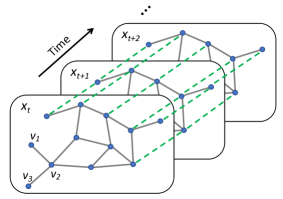
Figure 1: Spatio-temporal dependency modelling for traffic data, where grey lines and green dash lines represent spatial and temporal dependency, respectively.

Fig. 1 describes the spatio-temporal correlation modelling problem in traffic forecasting. Instead of treating the forecasting as deterministic, we aim to compute a conditional distribution to predict the traffic flow as well as the prediction uncertainty $\hat{X}_{>t}\sim P(\hat{X}_{>t}|X_{<t})$, which can improve the accuracy of the prediction, enhance the generalization ability of the model, and provide uncertainty estimation as well.

Note that although multi-modality and seasonality in traffic data do exist [6], for simplicity, we do not consider multi modality or seasonality, and consequently treat the predictive distribution of each node at each time point as a conditional uni-variate Gaussian distribution. A similar assumption can also be found in [36]. To this end, $P(\hat{X}_{>t}|X_{<t})$ can be represented by a set of predictive mean-variance pairs. As a result, the problem is cast as follows:

$$\theta=\underset{\theta}{\mathrm{argmax}}~{}\sum^{N}_{i=1}\log\mathcal{N}(\hat{X}^{i}_{>t};\hat{\mu}_{\theta}(X^{i}_{<t}),\hat{\sigma}_{\theta}(X^{i}_{<t})^{2}),$$ (1)

where $\theta$ is the model parameters, $N$ is the number of total training data points, $\mathcal{N}$ denotes the Gaussian likelihood, $\hat{\mu}(X_{<t})$ and $\hat{\sigma}(X_{<t})^{2}$ represents the estimated mean and variance, respectively.

IV Deep Spatio-Temporal Uncertainty Quantification

We first briefly give an overview of the proposed Deep Spatio-Temporal Uncertainty Quantification (DeepSTUQ). The DeepSTUQ model architecture is illustrated in Fig. 2, which follows the principle of [5]. This architecture includes an encoder and a decoder sub-neural network. The encoder is composed of a GCN and a GRU module to capture both the spatial and temporal dependencies, respectively. To estimate the aleatoric uncertainty, the decoder employs two independent convolutional layers computing means and variances, respectively. Moreover, dropout operations are deployed in both sub-networks to estimate the epistemic uncertainty.

In terms of model training, conventional training procedures are only capable of providing uni-modal solutions, which lacks diversity for quantifying uncertainty [14]. To address this issue, a three-stage training method is proposed, which can be briefed as follows.

• Stage 1: Pre-train the base spatial-temporal model with dropout on the training dataset to perform variational learning;

• Stage 2: Re-train the pre-trained model on the training dataset to proceed ensemble learning;

• Stage 3: Calibrate the re-trained model on the validation dataset to further improve the aleatoric variance estimation.

In the following sections, we will introduce DeepSTUQ in detail.

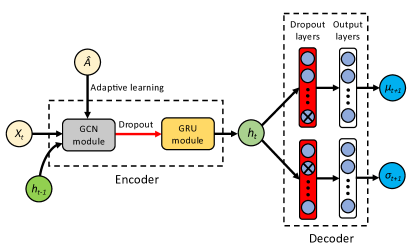
Figure 2: Architecture of DeepSTUQ.

IV-A Spatial Dependency

IV-A1 Graph Convolution

A typical road network consists of a number of road segments. The spatial relationships within a road network with $N_{R}$ road segments can be described through a graph $\mathcal{G(V,E)}$, where the nodes $\mathcal{V}=\{v_{1},v_{2},v_{3},\cdots,v_{\lvert{}\mathcal{V}\rvert{}}\}$ denote the sensors and the edges $\mathcal{E}$ denotes the road segment. $A\in\mathbb{R}^{\lvert{}\mathcal{V}\rvert{}\times\lvert{}\mathcal{V}\rvert{}}$ is the corresponding adjacency matrix. Subsequently, GCN [17] is utilized to model the spatial relationships of the traffic data. The output of the $l\text{-th}$ GCN layer, $Z^{(l+1)}$, can be computed by

$$Z^{(l+1)} =f(Z^{(l)},A),$$ (2)

where $Z^{(l)}$ is the input. More specifically, GCN first uses a degree matrix $D$ to avoid changing the scale of feature vectors by multiplying it with $A$. Afterwards, an identity matrix $I$ is used to sum up the neighboring nodes of a node as well as the node itself. As a result, the propagation rule of GCN is described as follows:

$$Z^{(l+1)}=S\big{(}(I+D^{-\frac{1}{2}}AD^{-\frac{1}{2}})Z^{(l)}W^{(l)}+b^{(l)}\big{)},$$ (3)

where $W^{(l)}$ is the weight matrix, $b^{(l)}$ is the bias, and $S$ is an activation function, e.g., sigmoid function.

IV-A2 Graph Structure Learning

In many real-world cases, we do not have the real spatial correlation knowledge of the multivariate traffic data. In such cases, the graph structure needs to be learned from data. To this end, the adaptive learning approach proposed in [5] is adopted to directly generate $\hat{A}=D^{-\frac{1}{2}}AD^{-\frac{1}{2}}$, which is easier than generating the adjacency matrix during the training process. Particularly, $\hat{A}$ is developed by

$$\hat{A}=\operatorname{softmax}\big{(}\operatorname{ReLU}(EE^{T})\big{)},$$ (4)

where $E\in\mathbb{R}^{\lvert{}\mathcal{V}\rvert{}\times d}$ (the embedding dimension $d\ll\lvert{}\mathcal{V}\rvert{}$) is a learnable matrix representing the embedding of the nodes and $\operatorname{softmax}$ function is to normalize the learned matrix. To facilitate the graph learning process, the Node Adaptive Parameter Learning (NAPL) module [5] is also utilized to reduce the computational cost. As a result, Equation (3) becomes

$$Z^{(l+1)}=S\big{(}(I+\hat{A})Z^{(l)}EW_{g}^{(l)}+Eb_{g}^{(l)}\big{)}.$$ (5)

IV-B Temporal Dependency

Apart from the spatial dependency, the temporal dependency of traffic data also needs to be captured. To this end, the aforementioned graph convolutional operations and adaptive graph learning module are integrated into a Gated Recurrent Unit (GRU) [20]. Subsequently, the obtained spatio-temporal model can be formulated as follows:

$$z_{t}=S\big{(}(I+\hat{A})[x_{t},h_{t-1}]EW_{z}+Eb_{z}\big{)},$$ (6a)

$$r_{t}=S\big{(}(I+\hat{A})[x_{t},h_{t-1}]EW_{r}+Eb_{r}\big{)},$$ (6b)

$$c_{t}=\tanh\big{(}(I+\hat{A})[x_{t},r_{t}\odot h_{t-1}]EW_{c}+Eb_{c}\big{)},$$ (6c)

$$h_{t}=z_{t}\odot h_{t-1}+(1-z_{t})\odot c_{t},$$ (6d)

where $z$ stands for the update gate, $r$ stands for the reset gate, $h$ denotes the hidden state, $\operatorname{[\cdot]}$ denotes the concatenation operation, $c$ denotes the memory cell, $W$ and $b$ represent the weights and bias, respectively.

Finally, the model introduced in Equation (6) serves as the spatio-temporal architecture in DeepSTUQ. Note that though the above base model is employed in this work, DeepSTUQ has the potential to be applied to other spatial-temporal structures as well. In the following sections, we explain how to leverage this base model to forecast traffic and quantify the corresponding forecasting uncertainty.

IV-C Uncertainty Quantification

Generally, uncertainty can be classified into two types, i.e., epistemic and aleatoric. The former represents model uncertainty, while the latter represents data uncertainty. If variance is used to render uncertainty, the total uncertainty can be decomposed and approximated as follows:

$$\sigma_{\text{Total}}^{2}\approx\underbrace{\mathbb{E}_{\theta\sim p(\theta)}[\sigma^{2}_{\theta}]}_{\text{Aleatoric uncertainty}}+\underbrace{\mathbb{V}_{\theta\sim p(\theta)}[\mu_{\theta}]}_{\text{Epistemic uncertainty}},$$ (7)

where $p(\theta)$ stands for a probability distribution over the model parameters $\theta$, $\sigma^{2}_{\theta}$ and $\mu_{\theta}$ refer to predicted variance and mean, respectively.

IV-C1 Aleatoric Uncertainty

Aleatoric uncertainty is caused by the intrinsic randomness of data, which is irreducible but learnable [27]. Based on Equation (7), we assume that the lower and upper bounds of the forecasting are symmetric due to the regressive nature of the prediction. Subsequently, the distribution of a sensor’s value, e.g., traffic flow, at each time point can be modeled by a Gaussian distribution with predicted mean $\mu(x)$ and variance $\sigma(x)^{2}$. However, directly maximizing the predictive Gaussian likelihood is numerically unstable. Instead we choose to maximize the following log-likelihood:

$$\log \;p(y|\mu(x),\sigma(x))$$

$$= \,-\frac{1}{2}\log(\sigma(x)^{2})-\frac{1}{2}\log(2\pi)-\frac{(y-\mu(x))^{2}}{2\sigma(x)^{2}},$$ (8)

where $\log(\sigma(x)^{2})$ and $\mu(x)$ are obtained directly via two independent neural networks.

In practice, to accelerate the training process and ensure convergence, we devise the following weighted loss by adding an L1 loss as the regularization term based on Equation (IV-C1):

$$\mathcal{L_{\text{Aleatoric}}}=\frac{1}{N}\sum^{N}_{i=1}\lambda \,\big{\{}\log(\sigma(x_{i})^{2})+\frac{(y_{i}-\mu(x_{i}))^{2}}{\sigma(x_{i})^{2}}\big{\}}$$

$$\,+(1-\lambda)|y_{i}-\mu(x_{i})|,$$ (9)

where $\lambda$ is the relative weight with $0<\lambda\leq 1$.

IV-C2 Epistemic Uncertainty

Epistemic uncertainty represents model uncertainty, which arises from that lack of data or model mis-specification. Fortunately, as opposed to aleatoric uncertainty, epistemic uncertainty can be reduced by estimation.There are two general classes of approaches to do so: Bayesian variational inference and deep ensembling. However, they both have their pros and cons. Fig. 3 illustrates the relationships between different solutions and corresponding model performance. The solid and dashed lines represent the model performance during training and testing processes, respectively. The green line and blue dots represent the performance that can be obtained by variational inference and deterministic model, respectively. As it can be seen from the figure, deep ensembling can find a set of different deterministic model parameters (local minimums), e.g., $W_{1}$, $W_{2}$, and $W_{3}$, which may have equally good performance in the solution space [37]. On the other hand, variational inference can find a set of sub-optimal solutions near one local minimum in the loss space. However, it may fail to find other local minimums, which potentially leads to modal collapse. Therefore, a better way is to explore as many as local minimums as well as their corresponding nearby solutions. To this end, we propose to combine deep ensembling and variational inference to estimate epistemic uncertainty.

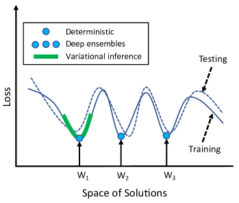
Figure 3: Performance demonstration of deterministic model, deep ensembles, and variational inference in solution space.

Variational Inference. Let $D=\{X,Y\}$ be the training dataset. From a Bayesian perspective, we assume each weight parameter of the neural network $w$ obeys a probabilistic distribution to represent model uncertainty, e.g., Gaussian distribution. However, in practice, the true posterior of the the neural network weights $p(w|D)$ is intractable. Therefore, a variational distribution $q(w)$ is used to approximate $p(w|D)$. Accordingly, the optimization goal is to minimize the following Kullback-Leibler (KL) divergence:

$$D_{\text{KL}}(q(w)||p(w|D))$$

$$=\int q(w)\log\frac{q(w)}{p(w)p(D|w)}dw,$$

$$=D_{\text{KL}}(q(w)||p(w))-\mathbb{E}_{w\sim q(w)}[\log p(D|w)],$$ (10)

where $p(w)$ is the prior and $\log p(D|w)$ is the predictive log-likelihood.

To solve Equation (IV-C2), MC dropout [30] is adopted as it performs Bayesian approximation in a simple and flexible manner. The variational distribution $q(w)$ formulated in MC dropout can be described as follows. Let $W_{i}$ be a matrix of shape $K_{j}\times K_{j-1}$ for layer $i$, we have

$$q(W_{i}) =M_{i}\cdot(\operatorname{diag}[z_{i,j}]^{K_{i}}_{j=1}),$$ (11a)

$$z_{i,j} \sim\operatorname{Bernoulli}(p_{i})$$ (11b)

where $W_{i}$ denotes the masked weight matrices, $p_{i}$ is dropout rate used in both the training and testing processes (as opposed to standard dropout), $M_{i}$ is the parameters of the neural network in the $i$-th layer , and $z_{i,j}$ is a binary variable indicating whether unit $j$ at layer $i-1$ (as the input of layer $i$) is dropped. As a result, minimizing Equation (IV-C2) is equivalent to minimizing the following loss function:

$$\mathcal{L_{\text{Dropout}}} =\mathbb{E}_{w\sim q(w)}E[Y,f_{W}(X)]-D_{\text{KL}}(q(w)||p(w)),$$

$$\approx\frac{1}{N}\sum_{i=1}^{N}E(y_{i},f(x_{i},w_{i}))+\frac{\lambda_{W}}{2p_{i}}||w_{i}||^{2},$$ (12)

where $E$ is the loss function, e.g., Root Mean Squared Error (RMSE) or Mean Absolute Error (MAE), $\lambda_{W}$ is the weight decay, and $\frac{\lambda_{W}}{2p}||w||^{2}$ can be computed through applying the L2 regularization during the training process.

In terms of implementation, dropout operations are deployed at two places within the spatial-temporal model: the graph convolutional layers in the encoder and the dropout convolutional layers in the decoder. Therefore, Equation (5) becomes

$$Z^{(l+1)}=\operatorname{sigmoid}\Big{(}M\odot\big{(}(I+\hat{A})Z^{(l)}EW_{g}^{(l)}+Eb_{g}^{(l)}\big{)}\Big{)}.$$ (13)

Note that the dropout rate here should be small when the adjacency matrix dimension is small, and vice versa.

Combined Uncertainty. Finally, Equations (IV-C2) and (IV-C1) are combined to estimate both aleatoric and epistemic uncertainty jointly. The combined loss function is formulated by

$$\mathcal{L_{\text{Combined}}}=\frac{1}{N} \sum_{i=1}^{N}\lambda\,\big{\{}\log(\sigma(x_{i})^{2})+\frac{(y_{i}-\mu(x_{i}))^{2}}{\sigma(x_{i})^{2}}\big{\}}$$

$$\,+(1-\lambda)|y_{i}-\mu(x_{i})|+\frac{\lambda_{W}}{2p}||w||^{2}.$$ (14)

Equation (IV-C2) is utilized to pre-train the spatio-temporal model in DeepSTUQ .

Deep Ensembling. In contrast to variational inference, deep ensembling aims to find a set of different local minimums and averages the output of each trained model as the final prediction. Deep ensembling is shown to be quite effective in practice, yet it is computationally expensive as multiple models are trained [32]. FGE [34] tackles this issue by using cycling learning rate to produce a set of different trained models in one learning process. However, FGE still needs to store multiple models for inference, which may result in high memory cost. To address this issue, SWA [15] adjusts the learning rate and averages the weights during the learning process to generate only one trained model to approximate FGE. In SWA, the model parameters are updated by

$$w_{\text{SWA}}=\frac{w_{\text{SWA}}\cdot n_{\text{models}}+w}{n_{\text{models}}+1},$$ (15)

where $w_{\text{SWA}}$ is the parameters of the SWA model and $n_{\text{models}}$ is the number of averaged models during training.

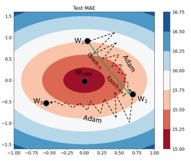
Figure 4: Demonstration of relationship between test MAEs and model weights during AWA re-training.

Inspired by SWA, we devise a re-training method called Adaptive Weight Averaging (AWA) to approximate deep ensembling. As depicted in Fig. 4, we vary the learning rate during the re-training process to find different local minimums, and average those local minimums in the final stage to attain better solutions. The proposed AWA re-training approach includes two steps. Let the re-training learning rate be $lr$, the maximum learning rate be $lr_{1}$, the minimum learning rate be $lr_{2}$, $n_{\text{iteration}}$ be the total iteration number within each epoch/total batch number, then the learning rate at $n_{i}$ iteration changes according to the following rules. The first step is to enable the trained model to escape from the current local minimum. To this end, the learning rate of the optimizer decreases from $lr_{1}$ to $lr_{2}$ via a cosine learning rate scheduler at epoch $n$. The scheduler is described by

$$lr=lr_{2}+\frac{1}{2}(lr_{1}-lr_{2})\big{(}1+\cos(\frac{n_{\text{iteration}}}{n_{i}}\pi)\big{)}.$$ (16)

Following that, the model is fine tuned by using the constant learning rate $lr_{2}$ at epoch $n+1$, then at the end of the epoch the model parameters are averaged according to Equation (15) and perform batch normalization. Specifically, we find that in practice using Adam as the optimizer works more effectively than using Stochastic Gradient Decent (SGD) which is adopted in the original SWA method. The learning rate change during the AWA re-training is illustrated in Fig. 5. The whole re-training process is summarized in Algorithm 1.

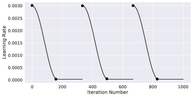
Figure 5: Learning rate change during the AWA re-training, each black dot indicates the start of a new epoch.

Algorithm 1 AWA Re-training Method

Require: training dataset {$X$}; pre-trained model parameters $w$; AWA model parameters $w_{\text{AWA}}$; learning rates: $lr_{1}$ and $lr_{2}$; total epoch $\text{epoch}_{\text{AWA}}$; total iteration/batch number $n_{\text{iteration}}$.

1:  while $\text{epoch}<\text{epoch}_{\text{AWA}}$:

2:   while $n<n_{\text{iteration}}$:

3:    compute the loss function according to Equation (IV-C2) and update $w$;

4:    if epoch $//$ 2 = 0:

5:     $lr$ decreases from $lr_{1}$ to $lr_{2}$ according to Equation (16);

6:    else: $lr=lr_{2}$;

7:   end while

8:   if epoch $//$ 2 = 0 and epoch $\neq$ 0:

9:    update $w_{\text{AWA}}$ according to Equation (15);

10:    perform batch normalization.

11:  end while

12:  Return $w_{\text{AWA}}$

At test time, we quantify the epistemic uncertainty by drawing multiple Monte Carlo samples from the learnt posterior distribution, then use the means and variances of the samples as the predictive mean and variances, respectively.

IV-C3 Model Calibration

To prevent the uncertainty estimation of the trained models being overconfident on the training dataset, it is necessary to calibrate the trained model on the validation dataset with post-processing.

To this end, a positive learnable variable $T$ is imposed on the learned variance. Subsequently, the following log-likelihood similar to Equation (IV-C1) is maximized:

$$\log \;p(y|\mu(x),\sigma(x)/T)$$

$$= \,\log(\frac{T}{\sigma(x)\sqrt{2\pi}}e^{-\frac{1}{2}((\frac{T(y-\mu(x))}{\sigma(x)})^{2}})$$

$$= \,\log(\frac{T}{\sigma(x)\sqrt{2\pi}})+\log(e^{-\frac{1}{2}(\frac{T(y-\mu(x))}{\sigma(x)})^{2}})$$

$$= \,-\frac{1}{2}\log(\frac{\sigma(x)^{2}}{T^{2}})-\frac{1}{2}\log(2\pi)-\frac{T^{2}(y-\mu(x))^{2}}{\sigma(x)^{2}}$$

$$= \,\frac{1}{2}\log(T^{2})-\frac{1}{2}\log(\sigma(x)^{2})-\frac{T^{2}(y-\mu(x))^{2}}{2\sigma(x)^{2}}-\frac{1}{2}\log(2\pi),$$ (17)

where $T$ is the only learnable parameter. Accordingly, the calibration objective is

$$T=\underset{T}{\mathrm{argmin}}\frac{1}{N}\sum_{i=1}^{N}- \log(T^{2})+\frac{T^{2}(y_{i}-\mu(x_{i}))^{2}}{\sigma(x_{i})^{2}},$$ (18)

where $\mu(x_{i})$ and $\sigma(x_{i})^{2}$ can be obtained via one deterministic forward pass or Monte Carlo estimation. Limited-memory Broyden-Fletcher-Goldfarb-Shanno algorithm (L-BFGS) is used as the optimizer to find the optimal value of $T$.

IV-D Proposed Unified Approach

Finally, combining the spatio-temporal correlation modelling method, Monte Carlo dropout, AWA re-training, and model calibration, the proposed unified uncertainty quantification method can be summarized as follows.

• First, the spatio-temporal model introduced in Section IV-A and IV-B is pre-trained using Equation (IV-C2) as the training loss function on the training dataset to estimate the aleatoric and epistemic uncertainty;

• Afterwards, the pre-trained model is re-trained via the AWA method on the training dataset to approximate deep ensembling;

• Finally, the predicted $\sigma^{2}$ obtained via the re-trained model on the validation dataset is calibrated according to Equation  (18).

The graphical probabilistic model representation of DeepSTUQ is visualized in Fig. 6. The figure shows that $h_{t}$ is extracted from $x_{t}$ via a spatio-temporal structure with a learnable variable $\hat{A}$. The model weights are drawn repeatedly to estimate the epistemic uncertainty, which is implemented in an efficient manner by using MC dropout and AWA. The variance $\sigma(x_{i})^{2}$ and mean $\mu(x_{i})$ are obtained via $N_{MC}$ Monte Carlo samples. Finally, $\sigma(x_{i})^{2}$ is calibrated through learning an auxiliary variable $T$.

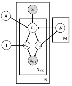
Figure 6: Graphical model representation of DeepSTUQ, where shaded circles represent observable variables, arrows denote dependencies, variables within rectangles appear repeatedly, $N_{MC}$ is the number of Monte Carlo samples, and $M$ is the number of models for ensembling.

At test time, according to Equation (7), we draw $N_{MC}$ Monte Carlo samples to estimate the predictive mean $\hat{\mu}_{t+1}$ and variance $\hat{\sigma}_{t+1}^{2}$ by

$$\hat{\mu}_{t+1} =\frac{1}{N_{MC}}\sum_{j=1}^{N_{MC}}\mu^{j}(x_{t}),$$ (19a)

$$\hat{\sigma}^{2}_{t+1} =\frac{1}{T}\sum_{j=1}^{N_{MC}}\frac{\sigma^{j}(x_{t})^{2}}{N_{MC}}+\sum_{j=1}^{N_{MC}}\frac{\big{(}\mu^{j}(x_{t})-\hat{\mu}_{t+1}\big{)}^{2}}{N_{MC}-1},$$ (19b)

where $\hat{\mu}_{t+1}$ is used as the point prediction of the proposed approach.

V Experiments

To compare the performance of DeepSTUQ with other state-of-the-arts, extensive experiments are conducted on real-world datasets in terms of point prediction, uncertainty quantification, and ablation study.

V-A Datasets

Four different public datasets collected from the Caltrans Performance Measurement System (PEMS), i.e., PEMS03, PEMS04, PEMS07, and PEMS08 [4] are used for evaluation. The traffic flow data aggregated to $5$ minutes. For prediction, one-hour historic data ($12$ data points) is utilized to predict the next’s ($12$ data points). All the datasets are split into three parts with ratio $6:2:2$ for training, validation/calibration, and testing, respectively. Table I summarizes the statistic of the four datasets.

TABLE I: Dataset statistic.

Dataset	# of Nodes	# of Edges	# of Steps
PEMS03	$358$	$547$	$26,208$
PEMS04	$307$	$340$	$16,992$
PEMS07	$883$	$866$	$28,224$
PEMS08	$170$	$295$	$17,856$

V-B Settings

Pre-training. The total number of training epochs is $100$. The optimizer is Adam with learning rate $0.003$ and weight decay $10^{-6}$. The batch size is $64$. The relative weight $\lambda$ in Equation (IV-C1) for computing the aleatoric uncertainty is $0.1$. The dropout rates of the graph convolutional operations in the encoder are $0.1$ for PEMS03, PEMS04, and PEMS07 (the adjacency matrice are relatively large), and $0.05$ for PEMS08 (the adjacency matrix is relatively small). The dropout rate at the final dropout layer in the decoder for all the datasets is $0.2$.

AWA Re-training. The optimizer of the AWA re-training process is Adam, and the maximum and minimum learning rates are $0.003$ and $0.00003$, respectively. The total number of re-training epochs is $20$, which means that $10$ models are averaged.

Model Calibration. The number of Monte Carlo samples for calculating $\sigma^{2}$ is $10$. The steps and numbers of iterations of the L-BFGS optimizer are $0.02$ and $500$, respectively.

Inference. To balance the inference time and model performance, we generate $10$ Monte Carlo samples for Bayesian approximation.

V-C Baselines

To compare the proposed DeepSTUQ with state-of-that-arts on point prediction and uncertainty quantification, two groups of recent traffic prediction methods are adopted as the baselines, respectively.

V-C1 Point Prediction Baselines

• DCRNN [1] adopts diffusion convolution and sequence-to-sequence learning;

• GraphWaveNet (GWN) [3] adopts a self-adaptive adjacency matrix and dilated casual convolution.

• ST-GCN [2] utilizes a GNN and a GCNN to forecast traffic;

• ASTGCN [6] employs Attention mechanism to model spatio-temporal dependency;

• STSGCN [4] forecasts traffic by synchronously extracting spatial-temporal correlations;

• STFGNN [24] employs a spatial-temporal fusion module and a gated dilated CNN;

• AGCRN [5] leverages a Node Adaptive Parameter Learning module and a Data Adaptive Graph Generation module to enhance traffic prediction performance;

• DeepSTUQ/S refers to the proposed method with single deterministic forward pass (dropout is turned off at test time).

V-C2 Uncertainty Quantification Baselines

Representative approaches of different uncertainty estimation paradigms (namely, frequentist, quantile prediction, Bayesian, and ensembling) are used as the baselines. Note that all the following methods employ the same base model structure for fair comparison.

• Point prediction refers to the AGCRN model which is used here to compare with other uncertainty quantification methods;

• Quantile regression [38] is a distribution-free method which directly computes the mean, lower and upper bounds using the corresponding quantile ($0.025$, $0.5$, $0.975$);

• Mean Variance Estimation (MVE) [12] refers to the method that estimates heterogeneous aleatoric uncertainty through computing Equation (IV-C1);

• Monte Carlo dropout (MCDO) [30] performs dropout at both training and test time, the number of Monte Carlo samples for inference is $10$;

• Combined refers to the method that calculates both epistemic and aleatoric uncertainty using Equation (IV-C2) [28], the number of Monte Carlo samples for inference is $10$;

• Temperature Scaling (TS) [16] calibrates the aleatoric uncertainty obtained by MVE;

• Fast Geometric Ensembling (FGE) [34] performs fast ensembling via varying the learning rate, the number of the stored trained models is $10$;

• Locally Weighted Conformal Inference [39], [40] calibrates the aleatoric uncertainty obtained by MVE via conformalization;

• Conformal Forecasting Recurrent Neual Network (CFRNN) [41] computes the multi-horizon uncertainty using conformal prediction;

TABLE II: Description of uncertainty quantification methods.

Method	Paradigm	Uncertainty Type
Point	deterministic	no
Quantile	distribution-free	aleatoric
MVE	frequentist	aleatoric
MCDO	Bayesian	epistemic
Combined	Bayesian	aleatoric + epistemic
TS	frequentist	aleatoric
FGE	ensembling	epistemic
Conformal	frequentist	aleatoric
CFRNN	distribution-free	aleatoric
DeepSTUQ	Bayesian + ensembling	aleatoric + epistemic

Table II summarizes the characteristics of the uncertainty quantification methods.

V-D Metrics

Two groups of metrics are employed to evaluate the point prediction and uncertainty quantification performance, respectively.

V-D1 Point Prediction Metrics

The point traffic forecasting performance are evaluated by the following metrics.

1. Root Mean Squared Error (RMSE):

   $$\mathrm{RMSE}=\sqrt{\frac{1}{N}\sum_{i=1}^{N}(\hat{y}_{i}-y_{i})^{2}},$$ (20)

   where $y_{i}$ is the ground truth, and $\hat{y}_{i}$ is the prediction.

2. Mean Absolute Error (MAE):

   $$\mathrm{MAE}=\frac{1}{N}\sum_{i=1}^{N}\left|\hat{y}_{i}-y_{i}\right|.$$ (21)

3. Mean Absolute Percentage Error (MAPE):

   $$\mathrm{MAPE}=\frac{1}{N}\sum_{i=1}^{N}\left|\frac{\hat{y}_{i}-y_{i}}{y_{i}}\right|.$$ (22)

V-D2 Uncertainty Quantification Metrics

The uncertainty quantification performance are evaluated by the following metrics.

1. Mean Negative Log-Likelihood (MNLL):

   $$\mathrm{MNLL}=\frac{1}{N}\sum_{i=1}^{N}-\log\mathcal{N}(y_{i};\hat{\mu}_{i},\hat{\sigma}^{2}_{i}),$$ (23)

   where $\hat{\mu}_{i}$ and $\hat{\sigma}^{2}_{i}$ are the predicted mean and predicted variance, respectively.

2. Prediction Interval Coverage Probability (PICP). The predicted lower and upper bounds of the prediction interval are denoted by $\hat{y_{L}}$ and $\hat{y_{U}}$, respectively. Let the significance level $\alpha$ be $5\%$, which means that the expected probability of a ground truth data point falling into the range $[\hat{y}_{L}$, $\hat{y}_{U}]$ is $95\%$ ($100\%-\alpha=95\%$). Accordingly, under Gaussianity assumption, $\hat{y}_{U_{i}}=\hat{\mu}_{i}+1.96\hat{\sigma}_{i}$, and $\hat{y}_{L_{i}}=\hat{\mu}_{i}-1.96\hat{\sigma}_{i}$. Let $k_{i}^{j}$ indicate whether the real speed value of a road segment $j$ at time $i$ is captured by the estimated prediction interval, and we have

   $$k_{i}=\begin{cases}1,\text{ if }\hat{y}_{L_{i}}\leq y_{i}\leq\hat{y}_{U_{i}}\\ 0,\text{ else}.\end{cases}$$ (24)

   Then PICP can be formulated by

   $$\mathrm{PICP}=\frac{1}{N}\sum_{i=1}^{N}k_{i}.$$ (25)

   Ideally, PICP should be equal or greater than $95\%$.

3. Mean Prediction Interval Width (MPIW):

   $$\mathrm{MPIW}=\frac{1}{N}\sum_{i=1}^{N}\hat{y}_{U_{i}}-\hat{y}_{L_{i}}.$$ (26)

V-E Point Prediction Results

TABLE III: Point prediction results on PEMS03, PEMS04, PEMS07, and PEMS08, where best and second best results are highlighted in bold and underlined, respectively.

Dataset	Metrics	DCRNN	ST-GCN	GWN	ASTGCN	STSGCN	STFGNN	AGCRN	DeepSTUQ/S	DeepSTUQ
PEMS03	MAE	$18.18$	$17.49$	$19.85$	$17.69$	$17.48$	$16.77$	$16.05$	$15.38$	$15.13$
	RMSE	$30.31$	$30.12$	$32.94$	$29.66$	$29.21$	$28.34$	$28.61$	$27.03$	$26.77$
	MAPE ($\%$)	$18.91$	$17.15$	$19.31$	$19.40$	$16.78$	$16.30$	$15.19$	$14.45$	$14.03$
PEMS04	MAE	$24.70$	$22.70$	$24.14$	$22.93$	$21.19$	$19.83$	$19.83$	$19.42$	$19.11$
	RMSE	$38.12$	$35.55$	$37.60$	$35.22$	$33.65$	$31.88$	$32.26$	$32.07$	$31.68$
	MAPE ($\%$)	$17.12$	$14.59$	$17.93$	$16.56$	$13.90$	$13.02$	$12.97$	$12.98$	$12.71$
PEMS07	MAE	$25.30$	$25.38$	$26.85$	$28.05$	$24.26$	$22.07$	$20.94$	$20.76$	$20.36$
	RMSE	$35.58$	$38.78$	$42.78$	$42.57$	$39.03$	$35.80$	$34.98$	$34.12$	$33.71$
	MAPE ($\%$)	$11.66$	$11.08$	$12.12$	$19.32$	$10.21$	$9.21$	$8.85$	$8.90$	$8.63$
PEMS08	MAE	$17.86$	$18.02$	$19.13$	$18.61$	$17.13$	$16.64$	$15.95$	$15.74$	$15.44$
	RMSE	$27.83$	$27.83$	$31.05$	$28.16$	$26.80$	$26.22$	$25.22$	$24.93$	$24.60$
	MAPE ($\%$)	$11.45$	$11.40$	$12.68$	$13.08$	$10.96$	$10.60$	$10.09$	$10.31$	$10.06$

The point prediction results of DeepSTUQ are compared with the aforementioned state-of-the-art methods first for performance evaluation. The obtained point prediction results are demonstrated in Table III. As it can be seen from the results, with only $10$ Monte Carlo samples, DeepSTUQ achieves the smallest RMSEs, MAEs, and MAPEs, which suggests that DeepSTUQ has the best performance on point traffic flow prediction. In addition, the proposed method — even with only one single deterministic forward pass, namely DeepSTUQ/S — also outperforms other state-of-the-art methods, which indicates that the proposed method is competitive on point prediction at nearly the same inference time cost as other deterministic approaches. This is because that variational inference can obtain a set of solutions around on one local minimum, and deep ensembling can find multiple local minimums in the solution space. By combining these two approaches, DeepSTUQ is capable of finding better sub-optimal solutions and have better generalization ability compared to deterministic methods, and consequently has better performance regarding point prediction. Fig. 7 shows the point prediction performance with respect to different horizons, which suggests that DeepSTUP has better performance than AGCRN at each time step for all the datasets.

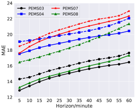
(a)

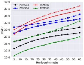
(b)

(c)

Figure 7: Point prediction results with respect to various forecast horizons, where solid and dashed lines denote DeepSTUQ and AGCRN, respectively. (a) MAE. (b) RMSE. (c) MAPE.

V-F Uncertainty Quantification Results

TABLE IV: Uncertainty quantification results on PEMS03, PEMS04, PEMS07, and PEMS08, the best results are highlighted in bold. The results are evaluated according to the following criteria. Any PICP $\geq 95\%$ is the best and the smallest corresponding MPIW is the best. If all the PICP $<95\%$, then the largest PICP is the best. MPIW only assessed when the corresponding PICP $\geq 95\%$.

Dataset	Metrics	Point	Quantile	MVE	MCDO	Combined	TS	FGE	Conformal	CFRNN	DeepSTUQ
PEMS03	MAE	$16.05$	$16.06$	$15.97$	$15.23$	$15.29$	$15.97$	$15.23$	$15.97$	$16.05$	$15.13$
	RMSE	$28.61$	$28.40$	$28.17$	$26.95$	$27.13$	$28.17$	$26.99$	$28.17$	$28.61$	$26.77$
	MAPE($\%$)	$15.19$	$15.50$	$15.08$	$14.39$	$14.60$	$15.08$	$14.36$	$15.08$	$15.19$	$14.03$
	MNLL	$-$	$-$	$3.53$	$12.32$	$3.39$	$3.49$	$25.94$	$3.53$	$-$	$3.38$
	PICP($\%$)	$-$	$89.49$	$92.06$	$43.92$	$93.64$	$93.51$	$31.15$	$93.21$	$93.00$	$94.75$
	MPIW	$-$	$65.60$	$74.04$	$19.73$	$73.26$	$79.79$	$12.81$	$76.72$	$82.79$	$76.91$
PEMS04	MAE	$19.83$	$20.08$	$19.86$	$19.15$	$19.23$	$19.86$	$19.08$	$19.86$	$19.83$	$19.11$
	RMSE	$32.26$	$32.76$	$32.30$	$31.49$	$31.73$	$32.30$	$31.59$	$32.30$	$32.26$	$31.68$
	MAPE($\%$)	$12.97$	$13.06$	$13.25$	$12.77$	$12.87$	$12.97$	$12.69$	$13.25$	$12.97$	$12.71$
	MNLL	$-$	$-$	$3.71$	$23.17$	$3.63$	$3.70$	$15.47$	$3.71$	$-$	$3.57$
	PICP($\%$)	$-$	$91.87$	$93.10$	$34.18$	$95.16$	$94.86$	$42.60$	$94.33$	$94.65$	$95.23$
	MPIW	$-$	$91.72$	$102.97$	$17.30$	$108.44$	$115.48$	$21.95$	$109.74$	$118.83$	$105.42$
PEMS07	MAE	$20.94$	$21.28$	$21.07$	$20.61$	$20.37$	$21.07$	$20.42$	$21.07$	$20.94$	$20.36$
	RMSE	$34.98$	$35.76$	$34.94$	$34.20$	$33.64$	$34.94$	$34.13$	$34.94$	$34.98$	$33.71$
	MAPE($\%$)	$8.85$	$8.95$	$8.88$	$8.73$	$8.68$	$8.88$	$8.622$	$8.88$	$8.85$	$8.63$
	MNLL	$-$	$-$	$3.80$	$9.88$	$3.60$	$3.78$	$22.31$	$3.80$	$-$	$3.60$
	PICP($\%$)	$-$	$91.83$	$93.86$	$53.74$	$95.80$	$95.53$	$38.05$	$94.78$	$94.65$	$95.74$
	MPIW	$-$	$96.63$	$112.99$	$31.16$	$112.36$	$127.00$	$19.03$	$118.79$	$118.83$	$111.68$
PEMS08	MAE	$15.95$	$16.40$	$16.29$	$15.87$	$15.51$	$16.29$	$15.79$	$16.29$	$15.95$	$15.44$
	RMSE	$25.22$	$25.79$	$25.71$	$25.05$	$24.64$	$25.71$	$24.96$	$25.71$	$25.22$	$24.60$
	MAPE($\%$)	$10.09$	$10.56$	$10.36$	$10.05$	$10.14$	$10.36$	$10.17$	$10.36$	$10.09$	$10.06$
	MNLL	$-$	$-$	$3.63$	$11.77$	$3.45$	$3.62$	$11.58$	$3.63$	$-$	$3.44$
	PICP($\%$)	$-$	$93.95$	$94.79$	$49.91$	$95.88$	$97.15$	$50.15$	$95.37$	$95.16$	$95.65$
	MPIW	$-$	$82.13$	$93.13$	$23.53$	$91.45$	$113.34$	$23.57$	$96.94$	$96.34$	$89.63$

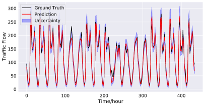
(a)

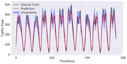
(b)

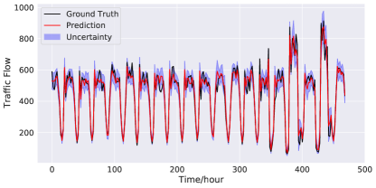
(c)

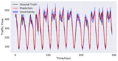
(d)

Figure 8: Uncertainty quantification results on randomly selected road segments from different datasets. (a) PEMS03. (b) PEMS04. (c) PEMS07. (d) PEMS08.

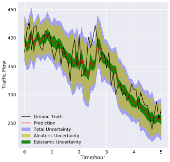
Figure 9: Quantification results of different uncertainties on partial data from a randomly selected segment of PEMS08.

(a)

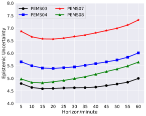
(b)

Figure 10: Uncertainty quantification results with respect to different horizons. (a) Aleatoric uncertainty. (b) Epistemic uncertainty.

To evaluate the uncertainty quantification performance, DeepSTUQ is compared with the uncertainty quantification baselines, whose results are demonstrated in Table IV and Figs. 8–10. According to the results in the table, the proposed approach has the best overall performance regarding both the point prediction and uncertainty quantification results compared with others. As it is observed from Fig. 8, DeepSTUQ can forecast traffic flow accurately and provide valid coverage for future ground truth. Fig. 9 illustrates that in traffic flow forecasting, the aleatoric uncertainty is much larger than the epistemic uncertainty. Hence, considering total uncertainty can provide better uncertainty estimation than considering either one alone. Fig. 10 shows that, for all the datasets, generally, both aleatoric and epistemic uncertainty increase as the prediction horizons extend, which implies that short-term traffic flow forecasting is more reliable than long-term one. The conclusion accords with the intuition and results in the literatures [1, 5, 24]

In terms of uncertainty quantification, the aleatoric uncertainty-aware approaches, i.e., MVE and TS, outperform the epistemic uncertainty-aware approaches, which suggests that the traffic uncertainty is mainly data-related. The results indicate that only considering epistemic uncertainty improves the estimation of the predictive mean (which results in better point estimation) but underestimates the variance significantly. This conclusion is supported by [35] as well. Although we have made a strong Gaussianity assumption on the likelihood of the aleatoric uncertainty, the obtained experimental results indicate that the methods using this assumption (i.e., MVE, Combined, TS, and DeepSTUQ) outperform the distribution-free method, Quantile. Additionally, the PICPs obtained by DeepSTUQ on the four datasets are very close to or larger than $95\%$, which implies that the Gaussian distribution assumption is credible.

According to the experimental results, we can also see that when only the epistemic uncertainty is considered using variational inference (MCDO) or deep ensembling (FGE), the traffic flow point prediction performance is improved compared to deterministic methods but the uncertainty quantification performance is poor. If merely the aleatoric uncertainty is taken into account (MVE, TS, Conformal, and CFRNN), the uncertainty quantification performance is satisfying while the point prediction slightly decreases compared to deterministic methods. On the other hand, if both the epistemic and aleatoric uncertainties are estimated, e.g., Combined and DeepSTUQ, the point prediction and uncertainty quantification performance are both improved.

V-G Ablation Study

Three groups of experiments are conducted to verify the effects of the proposed AWA training, the proposed model calibration method, and different numbers of Monte Carlo samples, respectively.

V-G1 Effect of AWA Re-training

The prediction performance of the same pre-trained model prior to and following AWA post-processing re-training are compared. Table V demonstrates that after AWA training, the point prediction performance has improved, indicating that the proposed AWA training method can approximate the deep ensembling method using only one single model with mere $20$ additional epochs. Therefore, compared to conventional deep ensembling, DeepSTUQ requires less time and memory.

TABLE V: Ablation study results on AWA training.

Dataset	Metrics	No AWA	AWA
PEMS03	MAE	$15.29$	$15.13$
	RMSE	$27.13$	$26.77$
	MAPE($\%$)	$14.60$	$14.03$
PEMS04	MAE	$19.23$	$19.11$
	RMSE	$31.73$	$31.68$
	MAPE($\%$)	$12.87$	$12.71$
PEMS07	MAE	$20.37$	$20.36$
	RMSE	$33.64$	$33.71$
	MAPE($\%$)	$8.68$	$8.63$
PEMS08	MAE	$15.51$	$15.44$
	RMSE	$24.64$	$24.60$
	MAPE($\%$)	$10.14$	$10.06$

V-G2 Effect of Model Calibration

The uncertainty quantification performance of the same model before and after applying the calibration method are compared. From the results illustrated in Tables VI and IV (results of MVE and TS), it can be seen that the uncertainty quantification performance has been further improved after model calibration, indicating that the proposed model calibration method is effective.

TABLE VI: Ablation study results on model calibration.

Dataset	Metrics	No Calibration	Calibration
PEMS03	MNLL	$3.39$	$3.38$
	PICP($\%$)	$94.22$	$94.75$
	MPIW	$74.51$	$76.91$
PEMS04	MNLL	$3.57$	$3.57$
	PICP($\%$)	$94.90$	$95.23$
	MPIW	$103.35$	$105.42$
PEMS07	MNLL	$3.60$	$3.60$
	PICP($\%$)	$95.38$	$95.74$
	MPIW	$108.85$	$111.68$
PEMS08	MNLL	$3.45$	$3.44$
	PICP($\%$)	$96.28$	$95.65$
	MPIW	$94.25$	$89.63$

V-G3 Effect of Monte Carlo Sample Number

To investigate how the number of Monte Carlo samples affects the model performance, the sample number is set to $1$, $3$, $5$, $10$ and $15$. As shown in Fig. 11, the performance of the proposed method enhances as the number of Monte Carlo samples rises, and only a small number of Monte Carlo samples are required to provide high prediction performance. The performance gradually saturates when the sample size approaches $15$. Accordingly, for the trade-off between the model performance and the inference time cost, the test-time sample number can be fixed to $10$ at test time.

(a)

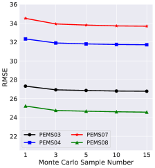
(b)

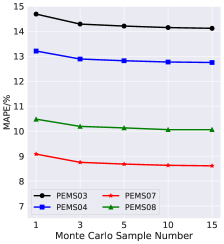
(c)

Figure 11: Prediction results with respect to different numbers of Monte Carlo samples. (a) MAE. (b) RMSE. (c) MAPE.

VI Conclusion

In this paper, we introduce a novel and unified uncertainty quantification method for traffic forecasting called DeepSTUQ. The proposed method consists of three components. 1) To model the aleatoric uncertainty, a hybrid loss function is used to train a base spatio-temporal model. 2) To model the epistemic uncertainty, the merits of variational inference and deep ensembling are combined through the dropout pre-training and AWA re-training. 3) The model is calibrated on the validation dataset using a post-processing calibration method based on Temperature Scaling to further improve the uncertainty estimation performance. Four distinct public datasets are then subjected to thorough experiments. The results indicate that DeepSTUQ outperforms contemporary state-of-the-art spatio-temporal models and uncertainty quantification methods.

Future research may include the incorporation of additional relevant information, e.g., weather forecasts, to enhance the traffic forecasting performance. Other deep learning techniques, such as Attention mechanism and hierarchical structures, are also worthy of investigation. The temporal and spatial features of traffic data at different scales are a promising future research direction, especially for long-term traffic prediction where multi-modality and seasonality play critical roles.

References

- [1] Y. Li, R. Yu, C. Shahabi, and Y. Liu, “Diffusion convolutional recurrent neural network: Data-driven traffic forecasting,” in International Conference on Learning Representations, 2018.
- [2] B. Yu, H. Yin, and Z. Zhu, “Spatio-temporal graph convolutional networks: a deep learning framework for traffic forecasting,” in Proceedings of the 27th International Joint Conference on Artificial Intelligence, 2018, pp. 3634–3640.
- [3] Z. Wu, S. Pan, G. Long, J. Jiang, and C. Zhang, “Graph wavenet for deep spatial-temporal graph modeling,” in Proceedings of the 28th International Joint Conference on Artificial Intelligence, 2019, pp. 1907–1913.
- [4] C. Song, Y. Lin, S. Guo, and H. Wan, “Spatial-temporal synchronous graph convolutional networks: A new framework for spatial-temporal network data forecasting,” in Proceedings of the AAAI Conference on Artificial Intelligence, vol. 34, no. 01, 2020, pp. 914–921.
- [5] L. Bai, L. Yao, C. Li, X. Wang, and C. Wang, “Adaptive graph convolutional recurrent network for traffic forecasting,” Advances in Neural Information Processing Systems, vol. 33, pp. 17 804–17 815, 2020.
- [6] S. Guo, Y. Lin, N. Feng, C. Song, and H. Wan, “Attention based spatial-temporal graph convolutional networks for traffic flow forecasting,” in Proceedings of the AAAI conference on artificial intelligence, vol. 33, no. 01, 2019, pp. 922–929.
- [7] C. Zheng, X. Fan, C. Wang, and J. Qi, “Gman: A graph multi-attention network for traffic prediction,” in Proceedings of the AAAI Conference on Artificial Intelligence, vol. 34, no. 01, 2020, pp. 1234–1241.
- [8] M. Veres and M. Moussa, “Deep learning for intelligent transportation systems: A survey of emerging trends,” IEEE Transactions on Intelligent transportation systems, vol. 21, no. 8, pp. 3152–3168, 2019.
- [9] S. Wang, J. Cao, and P. Yu, “Deep learning for spatio-temporal data mining: A survey,” IEEE transactions on knowledge and data engineering, 2020.
- [10] W. Jiang and J. Luo, “Graph neural network for traffic forecasting: A survey,” arXiv preprint arXiv:2101.11174, 2021.
- [11] Z. Wang, T. Xia, R. Jiang, X. Liu, K.-S. Kim, X. Song, and R. Shibasaki, “Forecasting ambulance demand with profiled human mobility via heterogeneous multi-graph neural networks,” in 2021 IEEE 37th International Conference on Data Engineering (ICDE). IEEE, 2021, pp. 1751–1762.
- [12] D. A. Nix and A. S. Weigend, “Estimating the mean and variance of the target probability distribution,” in Proceedings of 1994 ieee international conference on neural networks (ICNN’94), vol. 1. IEEE, 1994, pp. 55–60.
- [13] L. V. Jospin, W. Buntine, F. Boussaid, H. Laga, and M. Bennamoun, “Hands-on bayesian neural networks–a tutorial for deep learning users,” arXiv preprint arXiv:2007.06823, 2020.
- [14] J. Gawlikowski, C. R. N. Tassi, M. Ali, J. Lee, M. Humt, J. Feng, A. Kruspe, R. Triebel, P. Jung, R. Roscher et al., “A survey of uncertainty in deep neural networks,” arXiv preprint arXiv:2107.03342, 2021.
- [15] P. Izmailov, A. Wilson, D. Podoprikhin, D. Vetrov, and T. Garipov, “Averaging weights leads to wider optima and better generalization,” in 34th Conference on Uncertainty in Artificial Intelligence 2018, UAI 2018, 2018, pp. 876–885.
- [16] C. Guo, G. Pleiss, Y. Sun, and K. Q. Weinberger, “On calibration of modern neural networks,” in International Conference on Machine Learning. PMLR, 2017, pp. 1321–1330.
- [17] T. N. Kipf and M. Welling, “Semi-supervised classification with graph convolutional networks,” arXiv preprint arXiv:1609.02907, 2016.
- [18] M. Defferrard, X. Bresson, and P. Vandergheynst, “Convolutional neural networks on graphs with fast localized spectral filtering,” Advances in neural information processing systems, vol. 29, 2016.
- [19] P. Veličković, G. Cucurull, A. Casanova, A. Romero, P. Liò, and Y. Bengio, “Graph attention networks,” in International Conference on Learning Representations, 2018.
- [20] K. Cho, B. Van Merriënboer, C. Gulcehre, D. Bahdanau, F. Bougares, H. Schwenk, and Y. Bengio, “Learning phrase representations using rnn encoder-decoder for statistical machine translation,” arXiv preprint arXiv:1406.1078, 2014.
- [21] Y. N. Dauphin, A. Fan, M. Auli, and D. Grangier, “Language modeling with gated convolutional networks,” in International conference on machine learning. PMLR, 2017, pp. 933–941.
- [22] A. Van Den Oord, S. Dieleman, H. Zen, K. Simonyan, O. Vinyals, A. Graves, N. Kalchbrenner, A. W. Senior, and K. Kavukcuoglu, “Wavenet: A generative model for raw audio.” SSW, vol. 125, p. 2, 2016.
- [23] L. Zhao, Y. Song, C. Zhang, Y. Liu, P. Wang, T. Lin, M. Deng, and H. Li, “T-gcn: A temporal graph convolutional network for traffic prediction,” IEEE Transactions on Intelligent Transportation Systems, vol. 21, no. 9, pp. 3848–3858, 2019.
- [24] M. Li and Z. Zhu, “Spatial-temporal fusion graph neural networks for traffic flow forecasting,” in Proceedings of the AAAI conference on artificial intelligence, vol. 35, no. 5, 2021, pp. 4189–4196.
- [25] X. Zhang, C. Huang, Y. Xu, L. Xia, P. Dai, L. Bo, J. Zhang, and Y. Zheng, “Traffic flow forecasting with spatial-temporal graph diffusion network,” in Proceedings of the AAAI Conference on Artificial Intelligence, vol. 35, no. 17, 2021, pp. 15 008–15 015.
- [26] Z. Wu, S. Pan, G. Long, J. Jiang, X. Chang, and C. Zhang, “Connecting the dots: Multivariate time series forecasting with graph neural networks,” in Proceedings of the 26th ACM SIGKDD International Conference on Knowledge Discovery & Data Mining, 2020, pp. 753–763.
- [27] M. Abdar, F. Pourpanah, S. Hussain, D. Rezazadegan, L. Liu, M. Ghavamzadeh, P. Fieguth, X. Cao, A. Khosravi, U. R. Acharya et al., “A review of uncertainty quantification in deep learning: Techniques, applications and challenges,” Information Fusion, vol. 76, pp. 243–297, 2021.
- [28] A. Kendall and Y. Gal, “What uncertainties do we need in bayesian deep learning for computer vision?” arXiv preprint arXiv:1703.04977, 2017.
- [29] C. Blundell, J. Cornebise, K. Kavukcuoglu, and D. Wierstra, “Weight uncertainty in neural network,” in International conference on machine learning. PMLR, 2015, pp. 1613–1622.
- [30] Y. Gal and Z. Ghahramani, “Dropout as a bayesian approximation: Representing model uncertainty in deep learning,” in international conference on machine learning. PMLR, 2016, pp. 1050–1059.
- [31] N. Srivastava, G. Hinton, A. Krizhevsky, I. Sutskever, and R. Salakhutdinov, “Dropout: a simple way to prevent neural networks from overfitting,” The journal of machine learning research, vol. 15, no. 1, pp. 1929–1958, 2014.
- [32] B. Lakshminarayanan, A. Pritzel, and C. Blundell, “Simple and scalable predictive uncertainty estimation using deep ensembles,” Advances in neural information processing systems, vol. 30, 2017.
- [33] A. G. Wilson and P. Izmailov, “Bayesian deep learning and a probabilistic perspective of generalization,” Advances in neural information processing systems, vol. 33, pp. 4697–4708, 2020.
- [34] T. Garipov, P. Izmailov, D. Podoprikhin, D. P. Vetrov, and A. G. Wilson, “Loss surfaces, mode connectivity, and fast ensembling of dnns,” Advances in neural information processing systems, vol. 31, 2018.
- [35] D. Wu, L. Gao, X. Xiong, M. Chinazzi, A. Vespignani, Y.-A. Ma, and R. Yu, “Quantifying uncertainty in deep spatiotemporal forecasting,” arXiv preprint arXiv:2105.11982, 2021.
- [36] L. Zhu and N. Laptev, “Deep and confident prediction for time series at uber,” in 2017 IEEE International Conference on Data Mining Workshops (ICDMW). IEEE, 2017, pp. 103–110.
- [37] S. Fort, H. Hu, and B. Lakshminarayanan, “Deep ensembles: A loss landscape perspective,” arXiv preprint arXiv:1912.02757, 2019.
- [38] R. Koenker and K. F. Hallock, “Quantile regression,” Journal of economic perspectives, vol. 15, no. 4, pp. 143–156, 2001.
- [39] J. Lei, M. G’Sell, A. Rinaldo, R. J. Tibshirani, and L. Wasserman, “Distribution-free predictive inference for regression,” Journal of the American Statistical Association, vol. 113, no. 523, pp. 1094–1111, 2018.
- [40] A. N. Angelopoulos and S. Bates, “A gentle introduction to conformal prediction and distribution-free uncertainty quantification,” arXiv preprint arXiv:2107.07511, 2021.
- [41] K. Stankeviciute, A. M Alaa, and M. van der Schaar, “Conformal time-series forecasting,” Advances in Neural Information Processing Systems, vol. 34, pp. 6216–6228, 2021.