Abstract

We investigate the conditions for alignment in Dirac Gaugino models with minimal matter content. This leads to several scenarios, including an aligned Dirac Gaugino NMSSM that allows a light singlet scalar. We then investigate the compatibility of minimal Dirac Gaugino models with an enhanced W boson mass, using a new precise computation of the quantum corrections included in the code SARAH 4.15.0.

1 Introduction

While constraints on heavy Higgs bosons in supersymmetric models are rather stringent at large $\tan\beta$, excluding masses above a TeV, at small to moderate $\tan\beta$ direct searches do not place significant limits; only indirect constraints from $B\rightarrow s\gamma$ limit a heavy charged Higgs boson to be above $568$ GeV, roughly independent of $\tan\beta$ [1]. On the other hand, in the Minimal Supersymmetric Standard Model (MSSM), this region is likely excluded for an additional neutral Higgs boson below a few hundred GeV due to modifications to the SM-like Higgs boson couplings. This has led to a lot of interest in extensions of the MSSM (or variants of the Two Higgs Doublet Model) where alignment without decoupling is possible [2, 3, 4, 5, 6, 7, 8, 9], that is where the mixing between the SM-like Higgs boson and other scalars is minimised so that it aligns with the expectation values and has SM-like couplings.

Dirac Gaugino models [10, 11, 12, 13, 14, 15, 16, 17, 18], (see also, for example, [19, 20, 21, 22, 23, 24, 25, 26, 27, 28, 29, 30, 31, 32, 33, 34, 35, 36, 37, 38, 39, 40, 41, 42, 43, 44, 45, 46, 47, 48, 49, 50, 51, 52, 53, 54, 55, 56, 57, 58, 59, 60, 61, 62, 63, 64, 65]) accommodate scenarios where alignment without decoupling is automatic at tree-level[15, 66, 67, 68, 69, 70]. Under the assumption of an $N=2$ supersymmetry in the gauge sector at some scale, these models contain an approximate $SU(2)_{R}$ R-symmetry which guarantees the tree-level alignment [67]. An investigation of the effects of quantum corrections showed that it is even radiatively stable [66], with competing effects partially cancelling.

These models have many interesting phenomenological properties, and have been extensively studied in the literature. They involve, at a minimum, an extension of the MSSM by three adjoint chiral superfields, one for each gauge group; the fermions from these pair with the gauginos to give them a Dirac mass. This means the presence of new scalar fields, in singlet, triplet and octet representations.

Actually, it has not adequately been investigated to what extent the singlet could be light in such models. One condition for this to be the case is that it should not disturb the couplings of the light Higgs – in other words, we should have some amount of alignments without decoupling. ATLAS and CMS both give constraints on the overall signal strength of the Higgs boson $\mu$ to be [71, 72]:

$$\mu= 1.06\pm 0.07\ (\mathrm{ATLAS}),\qquad\mu=1.02^{+0.07}_{-0.06}\ (\mathrm{CMS}).$$ (1.1)

If the Higgs boson $h$ mixes with an inert singlet $s$, then we can write the mass eigenstates $\tilde{h},S$ as

$$\left(\begin{array}[]{c}h\\ s\end{array}\right)= \left(\begin{array}[]{cc}S_{11}&S_{12}\\ -S_{12}&S_{11}\end{array}\right)\left(\begin{array}[]{c}\tilde{h}\\ S\end{array}\right)$$ (1.8)

then we will find that

$$\mu= |S_{11}|^{2}\leq 1.$$ (1.9)

Hence if we allow a $3\sigma$ deviation from the ATLAS result, we require

$$1-|S_{11}|^{2}=|S_{12}|^{2}\leq 0.15\longrightarrow|S_{12}|<0.39.$$ (1.10)

While this still allows a moderate amount of mixing, the larger the mixing between the flavour eigenstates, the stronger the direct search bounds on the singlet will be. Therefore in this work we will consider the conditions for an approximate alignment in which the light Higgs mixes neither with the Heavy Higgs nor with the singlet (the triplet being decoupled). This will lead to a scenario that we refer to as the aligned DGNMSSM.

Recently, the CDF experiment reported a new measurement of the mass of the W boson [73]. Compared to the SM prediction [74, 75, 73], this gives as averages (combined Tevatron+LEP[76, 77, 78, 79, 80, 81, 82, 83, 73]):

$$M_{W}^{\rm Tevatron+LEP}= 80424\pm 9\ \mathrm{MeV},\qquad M_{W}^{\rm SM}=80356\pm 6\ \mathrm{MeV}.$$ (1.11)

If we take the central value of the top quark mass to be $172.89$ GeV then the central SM prediction becomes $80352$ MeV [84]. These differ by $7$ standard deviations, although measurements at the LHC [85, 86] also differ from the combination of Tevatron+LEP by $4$ standard deviations, so at this stage confirmation is required by other experiments. Nevertheless, a modification to the W boson mass is one of the most generic effects of new light particles coupling to the electroweak sector, so such a hint is tantalising.

It has generally been assumed in Dirac Gaugino models that the adjoint scalars should be heavy; indeed, the requirement that the triplet scalar vacuum expectation value (vev) must be very small compared to the Standard Model Higgs one – otherwise it would generate a large $\rho$ parameter - is usually ensured by giving the triplet a heavy mass. Amusingly, following the new measurement, the simplest explanation for the enhanced W boson mass is exactly an expectation value for the neutral component of such a triplet. In this work we shall investigate that possibility in minimal Dirac Gaugino models.

Such a triplet scalar also comes along with electroweak fermions, which can modify the quantum corrections too. Therefore a precise computation is required. While a preliminary such computation was performed for the MRSSM [87] using an update to FlexibleSUSY [88, 89], and a related computation was performed for the same model in [90], that model lacks a natural enhancement to the W boson quantum corrections. In this work we introduce a similarly precise computation in the package SARAH-4.15.0 and use it to examine the compatibility of our aligned DGNMSSM, along with four other scenarios – the “MSSM without $\mu$ term,” the MDGSSM, the aligned MDGSSM and the general DGNMSSM – with the new measurement of the W boson mass, or a naive world average value of $M_{W}^{\rm world\ average}=80411\pm 15$ MeV.

This work is organised as follows. In section 2 we summarise the essential details of the class of Dirac Gaugino models, including the vacuum minimisation conditions and mass matrices. The conditions for alignment are reviewed and a comparison is made with the cases of the MSSM and NMSSM. We also introduce the different variants we shall consider: the MSSM without $\mu$-term; the MDGSSM, the DGNMSSM and the aligned DGNMSSM. In Section 3 we will study the predictions for all of these classes of models for the W boson mass, examining in particular the effects of a precise computation of the quantum effects. We present our conclusions in section 4.

2 Dirac Gaugino Models with Automatic Tree-level Alignment

2.1 Field content and interactions

We shall consider in this work the extension of the MSSM by a minimal matter content to allow Dirac Gaugino masses, as in [18, 35]. The additional superfields consist of three chiral multiplets, in adjoint representations of the SM gauge group factors (DG-adjoints): a singlet $\mathbf{S}$, an $SU(2)_{W}$ triplet $\mathbf{T}^{a}$, and an $SU(3)_{C}$ octet $\mathbf{O}^{a}$. If we require gauge-coupling unification, even more states should be added to the model. For instance, for an $(SU(3))^{3}$ Grand Unification, the minimal set of chiral multiplets includes also extra Higgs-like doublets $\mathbf{R}_{u,d}$ as well as two pairs of vector-like right-handed electron $\mathbf{{E^{\prime}}}_{1,2}$ in $(\mathbf{1},\mathbf{1})_{1}$ and $\mathbf{\tilde{{E^{\prime}}}}_{1,2}$ in $(\mathbf{1},\mathbf{1})_{-1}$. We will not consider these states here.

In order to develop an intuition for the different interactions involved, it is helpful to consider a simple picture where the model descends from a supersymmetric theory in $D$ dimensions. The different states can appear in different sectors: some live in the whole $D$-dimensional bulk, others are localised on four-dimensional hyper-surfaces (branes) at points of the extra dimensions of coordinates $x_{i}=\{x^{a}_{i}\}$, $a=5,\cdots,D$. The corresponding Lagrangian can be written as

$$\int d^{D}x\,\,\mathcal{L}=\int d^{D}x\,\,\{\mathcal{L}_{bulk}+\sum_{i}\delta^{(D-4)}(x-x_{i})\,\,\,\,\mathcal{L}^{(i)}_{boundaries}\}~{},$$ (2.1)

where we have not explicitly written the metric factors. The four-dimensional theory arises after a truncation keeping only the compactification zero modes:

$$\mathcal{L}^{4d} = \mathcal{L}^{4d}_{bulk}+\mathcal{L}_{boundaries}~{},$$ (2.2)

$$\mathcal{L}^{4d}_{bulk} = \int d^{D-4}x\,\,\mathcal{L}_{bulk}~{},$$ (2.3)

$$\mathcal{L}_{boundaries} = \int d^{D-4}x\,\,\sum_{i}\delta^{(D-4)}(x-x_{i})\,\,\,\,\mathcal{L}^{(i)}_{boundaries}~{}.$$ (2.4)

A tree-level alignment in the Higgs sector appears in a class of models where the bulk theory leads to a four-dimensional Lagrangian with interactions governed by an $N=2$ extended SUSY. In particular, the SM gauge fields and the DG-adjoint fields arise as $N=2$ vector supermultiplets, and the two Higgs chiral superfields $\mathbf{H}_{d}$ and $\mathbf{H}_{d}$ form an $N=2$ hypermultiplet, interacting through the superpotential

$$\mathcal{L}^{4d}_{bulk}\supset\int d^{2}\theta\,\,\{\mu\,\,\mathbf{H}_{u}\cdot\mathbf{H}_{d}+\lambda_{S}\,\,\mathbf{S}\,\,\mathbf{H}_{u}\cdot\mathbf{H}_{d}+2\lambda_{T}\,\,\mathbf{H}_{d}\cdot\mathbf{T}\mathbf{H}_{u}\}~{},$$ (2.5)

where $\mathbf{T}\equiv\frac{1}{2}\sigma^{a}\,\mathbf{T}^{a}$, and the dot product is defined as

$$\mathbf{H}_{u}\cdot\mathbf{H}_{d}\equiv\epsilon_{ij}\mathbf{H}_{u}^{i}\mathbf{H}_{d}^{j}=\mathbf{H}_{u}^{+}\mathbf{H}_{d}^{-}-\mathbf{H}_{u}^{0}\mathbf{H}_{d}^{0}~{}.$$ (2.6)

The $N=2$ SUSY has a global $SU(2)_{R}$ R-symmetry that rotates between the generators of the two $N=1$ supercharges. The scalar components $S$, $T^{a}$ of $\mathbf{S}$ and $\mathbf{T}^{a}$, respectively, are singlets of $SU(2)_{R}$. This R-symmetry rotates then between the auxiliary fields $F_{\Sigma}^{a}$ of the adjoint superfields $\mathbf{\Sigma}^{a}\in\{\mathbf{S},\mathbf{T}^{a}\}$ and the auxiliary component $D^{a}$ of the corresponding chiral gauge superfields $\mathcal{W}^{a}_{i\,\alpha}$ for $U(1)_{Y}$ and $SU(2)_{W}$. This implies that

$$(\quad Re(F_{\Sigma}^{a})\quad,\quad D^{a}\quad,\quad{Im(F_{\Sigma}^{a})}\quad)$$ (2.7)

form a triplet of $SU(2)_{R}$. As a consequence, in order that the interactions (2.5) of $\mathbf{S}$ and $\mathbf{T}^{a}$ with the two Higgs doublets preserve $SU(2)_{R}$, the couplings $\lambda_{S}$ and $\lambda_{T}$ must be related through

$$\lambda_{S}=\frac{g_{Y}}{\sqrt{2}},\quad{\rm and}\quad\lambda_{T}=\frac{g_{2}}{\sqrt{2}}$$ (2.8)

to the couplings $g_{Y}$ and $g_{2}$ of the $U(1)_{Y}$ and $SU(2)_{W}$ gauge groups, respectively. Below the scale where the $N=2$ SUSY is broken to $N=1$, these relationships are spoiled by a small amount through renormalisation group running, so in numerical evaluations we must treat the couplings $\lambda_{S}$ and $\lambda_{T}$ as independent parameters.

In addition to the $SU(2)_{R}$ R-symmetry which is broken in $N=1$ (chiral) sectors, there is a global $U(1)_{R}$ R-symmetry under which the superspace coordinates $\theta^{\alpha}$ carry a $-1$ charge. The $U(1)_{R}$ charges of the $\mathbf{H}_{u}$ and $\mathbf{H}_{d}$ superfields are $R_{H_{u}}$ and $R_{H_{d}}$, respectively. They are arbitrary but subject to the constraint $R_{H_{u}}+R_{H_{d}}=2$. The DG-adjoint superfields $\mathbf{S},\mathbf{T}^{a}$, and $\mathbf{O}^{a}$ are R-neutral. Below, we shall classify the different $N=1$ interactions following whether they preserve or break the $U(1)_{R}$ symmetry.

The boundary Lagrangian can be split into different contributions:

$$\mathcal{L}^{4d}_{boundaries}~{}=~{}\mathcal{L}^{bulk}_{localised}+\int d^{2}\theta\,\,\{W_{Yukawa}+W_{DG}+W_{NR}\}\,+\,\Delta\mathcal{L}^{soft}\,.$$ (2.9)

Here, we denote by $\mathcal{L}^{bulk}_{localised}$ kinetic and interaction terms already present in the bulk theory $\mathcal{L}^{4d}_{bulk}$ but appearing with relative coefficients that violate $N=2$ supersymmetry. Such terms can a priori be present because the boundary theory preserves only $N=1$ SUSY, thus the coefficients of these terms are less constrained. Here, for simplicity, we assume such terms to vanish at tree level, to be only generated by quantum loops after supersymmetry breaking, and will therefore be accounted for in our analysis, at least in part, through the radiative corrections.

Also in (2.9), we have the usual MSSM Yukawa superpotential $W_{Yukawa}$ with the couplings responsible for the quark and lepton masses:

$$W_{Yukawa} = Y_{u}^{ij}\,\mathbf{U^{c}}_{i}\mathbf{Q}_{j}\cdot\mathbf{H}_{u}-Y_{d}^{ij}\,\mathbf{D^{c}}_{i}\mathbf{Q}_{j}\cdot\mathbf{H}_{d}-Y_{e}^{ij}\,\mathbf{E^{c}}_{i}\mathbf{L}_{j}\cdot\mathbf{H_{d}}~{},$$ (2.10)

which arises on the brane where the matter field supermultiplets are localised.

In this work, we consider a typical scale for the soft terms, for example squarks or gaugino masses, to be in the phenomenologically interesting range $m_{soft}\sim{\rm TeV}$. If we denote by $\Lambda$ a higher scale, for instance related to supersymmetry breaking messenger mass scale or to the Planck scale, then we can consider the relative strength of the diverse SUSY-breaking terms as an expansion in powers of $\frac{m_{soft}}{\rm\Lambda}$. We will assume that SUSY-breaking terms in the gauge sector preserve the $U(1)_{R}$ R-symmetry, giving rise to Dirac gaugino masses, while Majorana masses might be generated only by higher-order interaction terms, therefore suppressed by additional powers of hidden-sector couplings and/or $\frac{m_{soft}}{\rm\Lambda}$ where $\Lambda$ could be the Planck scale (for gravity-induced effects). The effective superpotential for the Dirac gaugino masses reads

$$W_{DG} = \sqrt{2}\theta^{\alpha}\bigg{[}m_{DY}\mathbf{S}\mathcal{W}_{1\,\alpha}+2m_{D2}\mathrm{tr}(\mathbf{T}\mathcal{W}_{2\,\alpha})+2m_{D3}\mathrm{tr}(\mathbf{O}\mathcal{W}_{3\,\alpha})\bigg{]}~{},$$ (2.11)

where $\mathbf{O}\equiv\frac{1}{2}\lambda^{a}\mathbf{O}^{a}$, and $\mathcal{W}_{i\,\alpha}$ are the chiral gauge-strength superfields. Finally, the superpotential $W_{NR}$ contains terms that break explicitly the $U(1)_{R}$ R-symmetry:

$$W_{NR} = \xi_{S}\,\mathbf{S}+\frac{M_{S}}{2}\,\mathbf{S}^{2}+\frac{\kappa}{3}\,\mathbf{S}^{3}+\lambda_{ST}\,\mathbf{S}\operatorname{tr}(\mathbf{T}\mathbf{T})+\lambda_{SO}\,\mathbf{S}\operatorname{tr}\left(\mathbf{O}\mathbf{O}\right)$$ (2.12)

$$+M_{T}\operatorname{tr}(\mathbf{T}\mathbf{T})+M_{O}\operatorname{tr}\left(\mathbf{O}\mathbf{O}\right)+\frac{\lambda_{O}}{3}\operatorname{tr}\left(\mathbf{O}\mathbf{O}\mathbf{O}\right)~{}.$$

The soft SUSY-breaking Lagrangian $\Delta\mathcal{L}^{soft}$ can in turn be split in two parts. The first contains the scalar mass and interaction terms that preserve the $U(1)_{R}$ R-symmetry:

$$-\Delta\mathcal{L}^{soft}_{R} = m_{H_{u}}^{2}\left|H_{u}\right|^{2}+m_{H_{d}}^{2}\left|H_{d}\right|^{2}+m_{S}^{2}|S|^{2}+2m_{T}^{2}\operatorname{tr}\left(T^{\dagger}T\right)+2m_{O}^{2}\operatorname{tr}\left(O^{\dagger}O\right)$$ (2.13)

$$+ (m_{Q}^{2})^{ij}Q^{\dagger}_{i}Q_{j}+(m_{U}^{2})^{ij}U^{c\dagger}_{i}U^{c}_{j}+(m_{D}^{2})^{ij}D^{c\dagger}_{i}D^{c}_{j}+(m_{L}^{2})^{ij}L^{\dagger}_{i}L_{j}+(m_{E}^{2})^{ij}E^{c\dagger}_{i}E^{c}_{j}$$

$$+ \biggr{(}t_{S}S+\frac{1}{2}B_{S}S^{2}+\frac{1}{3}T_{\kappa}S^{3}+T_{ST}S\,\mathrm{tr}(TT)+T_{SO}S\,\mathrm{tr}(OO)$$

$$~{}~{}~{}+B_{T}\,\operatorname{tr}(TT)+B_{O}\operatorname{tr}\left(OO\right)+\frac{1}{3}T_{O}\mathrm{tr}(OOO)+\text{h.c.}\biggr{)}~{}.$$

The second part of $\Delta\mathcal{L}^{soft}$ contains the scalar mass and interaction terms that break the $U(1)_{R}$ R-symmetry:

$$-\Delta\mathcal{L}^{soft}_{NR} \supset B_{\mu}\,H_{u}\cdot H_{d}+T_{S}\,SH_{u}\cdot H_{d}+2\,T_{T}\,H_{d}\cdot TH_{u}$$ (2.14)

$$+ T_{u}^{ij}\,{U^{c}}_{i}{Q}_{j}\cdot{H}_{u}-T_{d}^{ij}\,{D^{c}}_{i}{Q}_{j}\cdot{H}_{d}-T_{e}^{ij}\,{E^{c}}_{i}{L}_{j}\cdot{H_{d}}~{}+~{}\text{h.c.}~{},$$

as well as the Majorana mass terms $M_{i}$ (with $i=1,2,3$) for the gauginos. In general, the mechanisms that break R-symmetry and SUSY could be independent of each other, hence in eqs. (2.13) and (2.14) we refrained from defining the soft SUSY-breaking trilinear couplings as proportional to the corresponding superpotential couplings. In this work we assume that the soft SUSY-breaking Higgs-sfermion-sfermion interactions in the second line of eq. (2.14) are suppressed with respect to the R-conserving sfermion mass terms in eq. (2.13). This can be realised in our $D$-dimensional picture if the quark and lepton superfields are localised on a brane that differs from the one where the breaking of the R-symmetry takes place.

Since our study focuses on the electroweak sector of Dirac Gaugino models, we assume for simplicity that the scalar octet $O^{a}$ is heavy and can be integrated out of the theory. To insulate the singlet sector from threshold corrections involving the heavy octet, we also neglect the singlet-octet interaction term proportional to $\lambda_{SO}$ in the R-violating part of the superpotential, eq. (2.12), as well as the analogous term proportional to $T_{SO}$ in the R-conserving part of the soft SUSY-breaking Lagrangian, eq. (2.13). Similarly, since they cannot appear in some of our scenarios, for simplicity in the following we shall also neglect $\lambda_{ST},T_{ST}$ and the tadpole terms $t_{S},\xi_{S}$.

2.2 The electroweak scalar sector and alignment

We can now discuss the neutral scalar sector of this class of models. The vacuum expectation values  (vevs) of the neutral components of the doublets $H_{d}$ and $H_{u}$ are related by $v_{u}^{2}+v_{d}^{2}=v^{2}$, where $v\simeq 246$ GeV is the electroweak scale, and we define $\tan\beta=v_{u}/v_{d}$. The neutral singlet and triplet scalars $S$ and $T^{0}$ obtain vevs $\langle S\rangle=v_{S}/\sqrt{2}$ and $\langle T^{0}\rangle=v_{T}/\sqrt{2}$, respectively. These lead to effective $\mu$ and $B_{\mu}$ parameters:

$$\mu_{\rm eff} \equiv \mu+\frac{1}{\sqrt{2}}(\lambda_{S}v_{S}+\lambda_{T}v_{T}),$$ (2.15)

$$B_{\mu,\,\mathrm{eff}} \equiv B_{\mu}+\frac{1}{\sqrt{2}}(\lambda_{S}M_{S}+T_{S})v_{S}+\frac{1}{\sqrt{2}}(\lambda_{T}M_{T}+T_{T})v_{T}+\frac{1}{2}\lambda_{S}\kappa v_{S}^{2}.$$ (2.16)

The vevs $v_{S}$ and $v_{T}$ are then determined as a solution for the coupled cubic equations:

$$\kappa^{2}v_{S}^{3}+\frac{1}{\sqrt{2}}(T_{\kappa}+3\kappa M_{S})v_{S}^{2}+\tilde{m}_{SR}^{2}v_{S}~{}~{}~{}~{}~{}~{}~{}~{}~{}~{}~{}~{}~{}~{}~{}~{}~{}~{}~{}~{}~{}~{}~{}~{}~{}~{}~{}~{}~{}~{}~{}~{}~{}~{}~{}~{}~{}~{}~{}$$

$$+\frac{v^{2}}{2}\bigg{[}\sqrt{2}\lambda_{S}\mu_{\rm eff}-g_{Y}m_{DY}c_{2\beta}-(\frac{1}{\sqrt{2}}T_{S}+\frac{1}{\sqrt{2}}\lambda_{S}M_{S}+\lambda_{S}v_{S}\kappa)s_{2\beta}\bigg{]} = 0,$$ (2.17)

$$\tilde{m}_{TR}^{2}v_{T}+\frac{v^{2}}{2}\bigg{[}\sqrt{2}\lambda_{T}\mu_{\rm eff}+g_{2}m_{D2}c_{2\beta}-\frac{1}{\sqrt{2}}(T_{T}+\lambda_{T}M_{T})s_{2\beta}\bigg{]}~{}=~{}0,$$ (2.18)

where

$$\tilde{m}_{SR}^{2} \equiv M_{S}^{2}+m_{S}^{2}+B_{S}+4m_{DY}^{2},$$

$$\tilde{m}_{TR}^{2} \equiv M_{T}^{2}+m_{T}^{2}+B_{T}+4m_{D2}^{2},$$ (2.19)

are effective mass-squared parameters (at zero expectation value) for the real components $S_{R}$ and $T_{R}^{0}$ of the neutral singlet and triplet scalars (the analogous masses for the imaginary components $S_{I}$ and $T_{I}^{0}$ are $\tilde{m}_{SI}^{2}=M_{S}^{2}+m_{S}^{2}-B_{S}$ and $\tilde{m}_{TI}^{2}=M_{T}^{2}+m_{T}^{2}-B_{T}$, respectively). We know that $v_{T}$ must be small – namely, less than a few GeV – to avoid an overlarge tree-level $\Delta\rho$, so to a good approximation we can set $v_{T}=0$ in the vacuum minimisation equation for $v_{S}$, eq. (2.17), and decouple it from the one for $v_{T}$, eq. (2.18); this would allow the cubic equation for $v_{S}$ to be solved using standard techniques. However, the current state of technology for the computation of loop corrections assumes that we take expectation values as being valid for the true minimum of the full quantum-corrected potential, so in our numerical studies we must take them as inputs. Especially for $v_{T}$ this can lead to complications; see [91] for a recent discussion of this issue.

To discuss the alignment in the Higgs sector, it is now convenient to introduce the so-called Higgs basis for the two doublets,

$$\Phi_{1}\equiv\frac{v_{d}\Phi_{d}+v_{u}\Phi_{u}}{v},\quad\Phi_{2}\equiv\frac{-v_{u}\Phi_{d}+v_{d}\Phi_{u}}{v}~{},$$ (2.20)

where we defined for convenience two doublets with positive hypercharge, $\Phi_{u}^{j}\equiv H_{u}^{j}$ and $\Phi_{d}^{j}\equiv-\epsilon_{ij}H_{d}^{*j}$. In the Higgs basis the two doublets can be decomposed as

$$\Phi_{1}=\left(\begin{array}[]{c}G^{+}\\ (v+h+iG^{0})/\sqrt{2}\end{array}\right),\quad\Phi_{2}=\left(\begin{array}[]{c}H^{+}\\ (H+iA)/\sqrt{2}\end{array}\right)~{},$$ (2.21)

i.e., only the neutral component of $\Phi_{1}$ has a non-zero vev, and the would-be-Goldstone bosons, $G^{\pm}$ and $G^{0}$, all lie in $\Phi_{1}$. In general, the neutral CP-even fields $h$ and $H$ mix with the neutral CP-even components of the singlet and the triplet. In the basis $\{h,H,S_{R},T_{R}^{0}\}$, the tree-level mass matrix reads

$$\left(\mathcal{M}^{2}\right)_{\rm{\scriptscriptstyle tree}}= \left(\begin{array}[]{cccc}M_{Z}^{2}+\Delta_{h}s_{2\beta}^{2}&\Delta_{h}s_{2\beta}c_{2\beta}&\Delta_{hs}&\Delta_{ht}\\ \Delta_{h}s_{2\beta}c_{2\beta}&M_{A}^{2}-\Delta_{h}s_{2\beta}^{2}&\Delta_{Hs}&\Delta_{Ht}\\ \Delta_{hs}&\Delta_{Hs}&\tilde{m}_{S}^{2}&\lambda_{S}\lambda_{T}\frac{v^{2}}{2}\\ \Delta_{ht}&\Delta_{Ht}&\lambda_{S}\lambda_{T}\frac{v^{2}}{2}&\tilde{m}_{T}^{2}\end{array}\right),$$ (2.26)

where

$$\Delta_{h} = \frac{v^{2}}{2}(\lambda_{S}^{2}+\lambda_{T}^{2})-M_{Z}^{2},$$ (2.27)

$$\Delta_{hs} = v\bigg{[}\sqrt{2}\lambda_{S}\mu_{\rm eff}-g_{Y}m_{DY}c_{2\beta}-(\frac{1}{\sqrt{2}}(T_{S}+\lambda_{S}M_{S})+v_{S}\kappa\lambda_{S})s_{2\beta}\bigg{]}$$ (2.28)

$$\Delta_{Hs} = v\bigg{[}-(\frac{1}{\sqrt{2}}(T_{S}+\lambda_{S}M_{S})+v_{S}\kappa\lambda_{S})c_{2\beta}+g_{Y}m_{DY}s_{2\beta}\bigg{]},$$ (2.29)

$$\Delta_{ht} = v\bigg{[}\sqrt{2}\lambda_{T}\mu_{\rm eff}+g_{2}m_{D2}c_{2\beta}-\frac{1}{\sqrt{2}}(T_{T}+\lambda_{T}M_{T})s_{2\beta}\bigg{]},$$ (2.30)

$$\Delta_{Ht} = -v\bigg{[}\frac{1}{\sqrt{2}}(T_{T}+\lambda_{T}M_{T})c_{2\beta}+g_{2}m_{D2}s_{2\beta}\bigg{]},$$ (2.31)

$$M_{A}^{2} = \frac{2B_{\mu,\,\mathrm{eff}}}{s_{2\beta}},$$ (2.32)

$$\tilde{m}_{S}^{2} = \tilde{m}_{SR}^{2}+\lambda_{S}^{2}\frac{v^{2}}{2}-\kappa\lambda_{S}\frac{v^{2}}{2}s_{2\beta}+3\kappa^{2}v_{S}^{2}+\sqrt{2}v_{S}(T_{\kappa}+3\kappa M_{S}),$$ (2.33)

$$\tilde{m}_{T}^{2} = \tilde{m}_{TR}^{2}+\lambda_{T}^{2}\frac{v^{2}}{2}.$$ (2.34)

Exact alignment in the Higgs sector is obtained when one of the eigenstates of the CP-even mass matrix – in this work, we take it to be the lightest one – is aligned in field space with the direction of the SM Higgs vev, and thus has SM-like couplings to gauge bosons and matter fermions. This is equivalent to requiring that $h$ itself be an eigenstate of ${\cal M}^{2}$, or in other words that ${\cal M}^{2}_{1j}=0$ with $j=2,3,4$. If we make the reasonable assumption that the triplet is heavy, then this can be relaxed to just $j=2,3$. In addition, we will also refer in this work to cases where the singlet can be light without being potentially ruled out by direct searches. In this case we will require the supplementary condition that $\mathcal{M}^{2}_{23}=0$.

We start our discussion by focusing on the alignment between the two doublets. The use in eq. (2.27) of the $N=2$ condition for the singlet and triplet superpotential couplings, see eq. (2.8), implies $\Delta_{h}=0$ and $M_{h}=M_{Z}$, i.e. alignment is automatically realised at the tree level in this class of models, and the tree-level mass of the SM-like Higgs boson is independent of $\tan\beta$ but well below the value observed at the LHC. It is however well known that, in SUSY models, the radiative corrections to the Higgs mass matrix play a crucial role in lifting the prediction for the mass of the SM-like Higgs boson up to the observed value. Moreover, the radiative corrections to the condition in eq. (2.8) for the superpotential couplings of the adjoint superfields can become relevant if the scale $M_{N=2}$ where the $N=2$ SUSY is broken to $N=1$ is much larger than the scale where the Higgs mass matrix is computed. All of these corrections inevitably affect also the condition for alignment in the Higgs sector. As was discussed in ref. [66], in DG models the element that mixes the two doublets in the loop-corrected mass matrix can be recast as

$${\cal M}^{2}_{12}~{}=~{}\frac{1}{\tan\beta}\left[{\cal M}^{2}_{11}-M_{Z}^{2}\right]-\,\frac{v^{2}\,\tan\beta}{1+\tan^{2}\beta}\,\left[\left(\lambda_{S}^{2}-\frac{~{}g^{\prime\,2}}{2}\right)+\left(\lambda_{T}^{2}-\frac{g^{2}}{2}\right)\right]+\,(...)~{},$$ (2.35)

where ${\cal M}^{2}_{11}$ contains the dominant one-loop contribution from top and stops. The latter consists in a term enhanced by $y_{t}^{4}\,\ln(M_{{\rm\scriptscriptstyle SUSY}}^{2}/m_{t}^{2})$, where $y_{t}$ is the top Yukawa coupling and $M_{{\rm\scriptscriptstyle SUSY}}$ denotes for simplicity a common soft SUSY-breaking mass parameter for the stops. The second term in eq. (2.35) accounts for the deviation of the superpotential couplings from the $SU(2)_{R}$ condition in eq. (2.8), and the ellipses denote one-loop top/stop contributions that are suppressed by small ratios of parameters, one-loop contributions that involve couplings other than $y_{t}$, and higher-loop contributions. Close to alignment, the loop-corrected mass-matrix element ${\cal M}^{2}_{11}$ can be empirically identified with the observed mass of the SM-like Higgs boson, $M_{h}^{2}\approx 2\,M_{Z}^{2}$. Therefore, eq. (2.35) shows that the radiative corrections included in ${\cal M}^{2}_{11}$ tend to destroy the tree-level alignment in the Higgs sector of DG models. However, when $M_{N=2}$ is large the evolution of $\lambda_{S}$ and $\lambda_{T}$ down to the scale where the Higgs mass matrix is computed makes the second term in eq. (2.35) negative, and partially compensates for the misalignment induced by the top/stop contributions.

It is instructive to compare the condition for doublet alignment in DG models with the analogous conditions in the MSSM and in the NMSSM. In the case of the MSSM, discussed e.g. in refs. [6, 92], one finds

$${\cal M}^{2}_{12}~{}=~{}\frac{1}{\tan\beta}\left[{\cal M}^{2}_{11}-M_{Z}^{2}\,c_{2\beta}\right]+\,\frac{6\,y_{t}^{2}\,m_{t}^{2}\,\mu\,A_{t}}{16\pi^{2}\,M_{{\rm\scriptscriptstyle SUSY}}^{2}}\,\left(1-\frac{A_{t}^{2}}{6\,M_{{\rm\scriptscriptstyle SUSY}}^{2}}\right)\,+\,(...)~{},$$ (2.36)

where $A_{t}\equiv T_{u}^{33}/y_{t}$ is the soft SUSY-breaking Higgs-stop-stop interaction parameter, and again the ellipses denote sub-dominant terms. It appears that, in the MSSM, the alignment condition ${\cal M}^{2}_{12}=0$ can be realised radiatively when a large value of $\tan\beta$ suppresses the first term in eq. (2.36), while the parameters $M_{{\rm\scriptscriptstyle SUSY}}$, $A_{t}$ and $\mu$ combine in such a way that the second term is large and negative. In contrast, in DG models the contributions to ${\cal M}^{2}_{12}$ analogous to the second term in eq. (2.36) are suppressed by the assumption that $A_{t}\ll M_{{\rm\scriptscriptstyle SUSY}}$, see the comments after eq. (2.14), thus doublet alignment cannot be realised in this way. We remark however that, even with the $N=2$ condition for the superpotential couplings, in DG models ${\cal M}^{2}_{12}$ is smaller by a factor between $2$ and $3$ – depending on $\tan\beta$, which we assume to be greater than $1$ – with respect to the case of the MSSM with small $A_{t}$.

In the case of the NMSSM, discussed e.g. in refs. [7, 9], the mixing between $h$ and $H$ is given by

$${\cal M}^{2}_{12}~{}=~{}\frac{1}{\tan\beta}\left[{\cal M}^{2}_{11}-M_{Z}^{2}\,c_{2\beta}-\lambda_{S}^{2}\,v^{2}s^{2}_{\beta}\right]+\,\frac{6\,y_{t}^{2}\,m_{t}^{2}\,\tilde{\mu}\,A_{t}}{16\pi^{2}\,M_{{\rm\scriptscriptstyle SUSY}}^{2}}\,\left(1-\frac{A_{t}^{2}}{6\,M_{{\rm\scriptscriptstyle SUSY}}^{2}}\right)\,+\,(...)~{},$$ (2.37)

where $\tilde{\mu}\equiv\mu+\lambda_{S}\,v_{S}/\sqrt{2}$. Comparing with the case of the MSSM, eq. (2.36), we see that the condition ${\cal M}^{2}_{12}=0$ can be realised even in the absence of a large contribution from the terms proportional to $\mu_{\rm eff}A_{t}/M_{{\rm\scriptscriptstyle SUSY}}^{2}$, as long as the singlet-doublet superpotential coupling takes values in the range $\lambda_{S}^{2}\approx(3\!-\!4)\,M_{Z}^{2}/v^{2}$, where the exact numerical coefficient depends on the value of $\tan\beta$. As first pointed out in ref. [7], this condition singles out the region of the NMSSM parameter space where $\lambda_{S}\approx 0.7\pm 0.05$, a much larger value than would be implied by the $SU(2)_{R}$ condition in DG models.

To summarise, the $SU(2)_{R}$ R-symmetry implies exact alignment at the tree level in the Higgs-doublet sector of the DG models, but the alignment is partially spoiled by the radiative corrections that are necessary to obtain a realistic value for the SM-like mass. Alignment in the MSSM can be realised only through radiative corrections, for large $\tan\beta$ and for specific choices of the parameters in the stop sector. Finally, doublet alignment in the NMSSM can be realised even without the help of radiative corrections for an appropriate choice of $\lambda_{S}$, which – differently from the DG case with $SU(2)_{R}$ R-symmetry – is treated as a free parameter.

The second condition for Higgs alignment in DG models is ${\cal M}^{2}_{13}=0$, i.e. vanishing mixing between $h$ and $S_{R}$. Including the dominant contributions from stop loops, we find:

$$\mathcal{M}_{13}^{2}~{}=~{}\Delta_{hs}-\frac{6y_{t}\lambda_{S}c_{\beta}}{16\pi^{2}}m_{t}(A_{t}-\mu_{\rm eff}\cot\beta)\ln\frac{M_{{\rm\scriptscriptstyle SUSY}}^{2}}{Q^{2}}\,+\,(...)~{},$$ (2.38)

where the tree-level mixing term $\Delta_{hs}$ is given in eq. (2.28), $\mu_{\rm eff}$ is given in eq. (2.15), and $Q$ is the renormalisation scale at which the parameters entering $\Delta_{hs}$ are expressed. We assumed again a common soft SUSY-breaking mass term $M_{{\rm\scriptscriptstyle SUSY}}$ for the stops, and we neglected terms suppressed by powers of $m_{t}^{2}/M_{{\rm\scriptscriptstyle SUSY}}^{2}$. The various terms that contribute to $\Delta_{hs}$ arise from different sectors of the $D$-dimensional picture discussed earlier in this section: namely, $\mu$ and $\lambda_{S}$ enter the bulk superpotential in eq. (2.5); $m_{1D}$ enters the R-conserving boundary superpotential in eq. (2.11); $M_{S}$ and $\kappa$ enter the R-violating boundary superpotential in eq. (2.12); $T_{S}$ enters the R-violating SUSY-breaking Lagrangian in eq. (2.14). Therefore, even if we assume the $N=2$ SUSY relation of eq. (2.8) between $\lambda_{S}$ and $g_{Y}$, a vanishing $\mathcal{M}_{13}^{2}$ can only result from an accidental cancellation between unrelated terms. We also note that, in contrast to the case of $\mathcal{M}_{12}^{2}$, the radiative correction to $\mathcal{M}_{13}^{2}$ is not enhanced by $\tan\beta$ with respect to the tree-level part. Thus, its qualitative impact on our discussion of the alignment conditions is limited, as long as the scale $Q$ is not too far from $M_{{\rm\scriptscriptstyle SUSY}}$.

The minimum conditions of the scalar potential can be exploited to express the mass parameters for the doublets and the singlet in terms of the other Lagrangian parameters and of the vevs $v_{d}$, $v_{u}$ and $v_{S}$. In particular, we obtain a relation between the mass parameter $\tilde{m}_{SR}^{2}$ for the real component of the singlet, see eq. (2.2), and the matrix element $\mathcal{M}_{13}^{2}$ given in eq. (2.38):

$$\tilde{m}_{SR}^{2}~{}=~{}-\frac{v}{2\,v_{S}}\,\mathcal{M}_{13}^{2}-\frac{v_{S}}{\sqrt{2}}\left(T_{\kappa}+\sqrt{2}\kappa^{2}v_{S}+3\kappa M_{S}\right)\,~{}.$$ (2.39)

Eq. (2.39) above shows that the condition of vanishing mixing between $h$ and $S_{R}$, however realised, carries implications for the mass of the singlet. The diagonal element for the singlet in the scalar mass matrix is

$$\mathcal{M}_{33}^{2} = \tilde{m}_{SR}^{2}\,+\,\frac{1}{2}\lambda_{S}^{2}v^{2}\,+\,\sqrt{2}T_{\kappa}v_{S}\,+\,\kappa\left(3\kappa v_{S}^{2}+3\sqrt{2}M_{S}v_{S}-\lambda_{S}s_{\beta}c_{\beta}v^{2}\right)$$ (2.40)

$$+\frac{3y_{t}^{2}\lambda_{S}^{2}c_{\beta}^{2}}{32\pi^{2}}v^{2}\ln\frac{M_{{\rm\scriptscriptstyle SUSY}}^{2}}{Q^{2}}\,+\,(...)~{},$$

where we applied the same approximations as in eq. (2.38) for the one-loop correction in the second line.

We now discuss the simplest case in which the global $U(1)_{R}$ R-symmetry is preserved in the superpotential but broken by soft SUSY-breaking terms, in which case we can set $\kappa$ to zero. Since this implies a vanishing quartic self-coupling for the singlet, the stability of the scalar potential requires that we also assume $T_{\kappa}=0$, even if the trilinear self-coupling of the singlet resides in the R-conserving part of the soft SUSY-breaking Lagrangian. In this scenario, which we shall refer to as the aligned MDGSSM, eq. (2.39) shows that the alignment condition $\mathcal{M}_{13}^{2}\approx 0$ requires $\tilde{m}_{SR}^{2}\approx 0$ or $v_{S}\ll v$. The first of these two options implies that the CP-even mass eigenstate that is mostly singlet is relatively light: setting $\tilde{m}_{SR}^{2}=0$ and $\kappa=T_{\kappa}=0$ in eq. (2.40), and neglecting the small effect of the one-loop correction, we find that the value $\lambda_{S}\approx 0.7$ favored by the alignment condition for the Higgs doublets in the NMSSM, see eq. (2.38), leads to $\mathcal{M}_{33}^{2}\approx(122~{}{\rm GeV})^{2}$, whereas the value $\lambda_{S}\approx 0.25$ implied in our Dirac-gaugino model by the $N=2$ SUSY relation of eq. (2.8) leads to $\mathcal{M}_{33}^{2}\approx(44~{}{\rm GeV})^{2}$. We remark that the mixing between $S_{R}$ and the heavier, non-SM-like scalar $H$, which is controlled by $\mathcal{M}_{23}^{2}$, is suppressed when $M_{A}^{2}\gg\mathcal{M}_{33}^{2}$, and would in any case lower the mass of the singlet-like eigenstate.

The definition in eq. (2.2) shows that even the vanishing of $\tilde{m}_{SR}^{2}$ requires a cancellation between terms that arise from different sectors of our $D$-dimensional construction: $m_{1D}$ from the R-conserving boundary superpotential in eq. (2.11), $M_{S}$ from the R-violating boundary superpotential in eq. (2.12), $m_{S}^{2}$ and $B_{S}$ from the R-conserving soft SUSY-breaking Lagrangian in eq. (2.13). If such cancellation is not realised, the alternative requirement for alignment implied by eq. (2.39) when $\kappa=0$ is that $v_{S}\ll v$. This is not problematic as long as a suitable higgsino mass is provided by the $\mu$ term in the bulk superpotential, see eq. (2.5).

Finally, the third condition for Higgs alignment in DG models is ${\cal M}^{2}_{14}=0$, i.e. vanishing mixing between $h$ and $T^{0}_{R}$. The formulas for the relevant mass-matrix elements and for the minimum condition, including the dominant one-loop corrections from top and stop loops, are similar to eqs. (2.38)–(2.40), with the obvious singlet-to-triplet replacements but without terms analogous to those controlled by $\kappa$ in the singlet case:

$$\mathcal{M}_{14}^{2} = \Delta_{ht}-\frac{6y_{t}\lambda_{T}c_{\beta}}{16\pi^{2}}m_{t}(A_{t}-\mu_{\rm eff}\cot\beta)\ln\frac{M_{{\rm\scriptscriptstyle SUSY}}^{2}}{Q^{2}}\,+\,(...)~{},$$ (2.41)

$$\mathcal{M}_{44}^{2} = \tilde{m}_{TR}^{2}\,+\,\frac{1}{2}\lambda_{T}^{2}v^{2}\,+\,\frac{3y_{t}^{2}\lambda_{T}^{2}c_{\beta}^{2}}{32\pi^{2}}v^{2}\ln\frac{M_{{\rm\scriptscriptstyle SUSY}}^{2}}{Q^{2}}\,+\,(...)~{},$$ (2.42)

$$\tilde{m}_{TR}^{2}~{}=~{}-\frac{v}{2\,v_{T}}\,\mathcal{M}_{14}^{2}~{}.$$ (2.43)

The discussion of the constraints on the triplet mass induced by the condition of doublet-triplet alignment follows the lines of the discussion of singlet-triplet alignment for $\kappa=0$, with the important difference that the condition $v_{T}\ll v$ must in any case be satisfied to avoid an excessive contribution to $\Delta\rho$. As a consequence, it is not necessary to require $\tilde{m}_{TR}^{2}\approx 0$ to obtain approximate alignment. Nevertheless, we remark that the condition of exact alignment $\mathcal{M}_{14}^{2}=0$ would imply $\mathcal{M}_{44}^{2}\approx M_{W}^{2}$ through eqs. (2.41)–(2.43).

2.3 The electroweak fermion sector

We now outline the mass spectrum of the electroweak fermions, which will be relevant for our discussion examining the $W$ boson mass. The neutralino mass matrix, in the basis $\tilde{S},\tilde{B},\tilde{T}^{0},\tilde{W}^{0},\tilde{H}_{d}^{0},\tilde{H}_{u}^{0}$ reads:

$${\scriptsize\left(\begin{array}[]{c c c c c c}M_{S}+\sqrt{2}\kappa v_{S}&m_{DY}&0&0&-\frac{\sqrt{2}\lambda_{S}}{g_{Y}}M_{Z}s_{W}s_{\beta}&-\frac{\sqrt{2}\lambda_{S}}{g_{Y}}M_{Z}s_{W}c_{\beta}\\ m_{DY}&M_{1}&0&0&-M_{Z}s_{W}c_{\beta}&M_{Z}s_{W}s_{\beta}\\ 0&0&M_{T}&m_{D2}&-\frac{\sqrt{2}\lambda_{T}}{g_{2}}M_{Z}c_{W}s_{\beta}&-\frac{\sqrt{2}\lambda_{T}}{g_{2}}M_{Z}c_{W}c_{\beta}\\ 0&0&m_{D2}&M_{2}&M_{Z}c_{W}c_{\beta}&-M_{Z}c_{W}s_{\beta}\\ -\frac{\sqrt{2}\lambda_{S}}{g_{Y}}M_{Z}s_{W}s_{\beta}&-M_{Z}s_{W}c_{\beta}&-\frac{\sqrt{2}\lambda_{T}}{g_{2}}M_{Z}c_{W}s_{\beta}&M_{Z}c_{W}c_{\beta}&0&-\mu_{\rm eff}\\ -\frac{\sqrt{2}\lambda_{S}}{g_{Y}}M_{Z}s_{W}c_{\beta}&M_{Z}s_{W}s_{\beta}&-\frac{\sqrt{2}\lambda_{T}}{g_{2}}M_{Z}c_{W}c_{\beta}&-M_{Z}c_{W}s_{\beta}&-\mu_{\rm eff}&0\\ \end{array}\right)}$$ (2.44)

The chargino masses, $-\frac{1}{2}((v^{-})^{T}\mathcal{M}_{\chi^{\pm}}v^{+}+h.c.)$ in the basis $v^{+}=(\tilde{T}^{+},\tilde{W}^{+},\tilde{H}^{+}_{u})$, $v^{-}=(\tilde{T}^{-},\tilde{W}^{-},\tilde{H}^{-}_{d})$, are given by

$$\mathcal{M}_{\chi^{\pm}}=\left(\begin{array}[]{c c c}M_{T}&m_{D2}+g_{2}v_{T}&\lambda_{T}vc_{\beta}\\ m_{D2}-g_{2}v_{T}&M_{2}&\frac{g_{2}v}{\sqrt{2}}s_{\beta}\\ -\lambda_{T}vs_{\beta}&\frac{g_{2}v}{\sqrt{2}}c_{\beta}&\mu_{\rm eff}-\sqrt{2}\lambda_{T}v_{T}\\ \end{array}\right)$$ (2.45)

and do not depend on $\kappa$, but we have written for completeness the Majorana gaugino masses $M_{1,2}$ for the bino and wino respectively.

2.4 Scenarios

We have described the general features of minimal Dirac Gaugino models, and explained how some values of the couplings allow Higgs alignment to automatically occur at tree-level. Below, we shall consider the following different scenarios corresponding to specific choices of the model parameters:

• General MDGSSM

  In the general MDGSSM, the only source of $R$-symmetry violation comes from a small $B_{\mu}$ term, which is a radiatively stable condition (the renormalisation group running will not generate other $R$-symmetry violating terms from a $B_{\mu}$ term). This excludes all of $W_{NR}$; the only supersymmetric parameters beyond those of the MSSM retained are $\lambda_{S},\lambda_{T}$, but those are allowed to have any value. Supersoft masses [13] are allowed, and soft supersymmetry-breaking masses are allowed, but squark/sfermion trilinears and $T_{S},T_{T}$ are not. On the other hand, trilinears involving the adjoint scalars may be allowed (so $T_{\kappa},T_{ST},T_{SO}$) but may be argued to be small in typical models. The couplings $\lambda_{S},\lambda_{T}$ enhance the Higgs mass and W mass at the same time; while large values of $\lambda_{T}$ were previously deemed problematic for the $\rho$ parameter, they are now a virtue.

• MSSM without $\mu$ term (RIP)

  This model, described in [14], is identical to the general MDGSSM execpt that the $\mu$-term is set to zero (although a small $v_{S}$ generates a tiny effective $\mu$). In the MSSM this would yield massless higgsinos, but here the higgsinos obtain a mass through $\lambda_{T}$ which causes them to mix with the triplet fermion. Thus the $\mu$ problem of the MSSM is solved, at the expense of an upper bound on the chargino masses, which, as we shall see, leads to the model being ruled out.

• Aligned MDGSSM

  By taking $\lambda_{S},\lambda_{T}$ to their their $N=2$ values given in Eq. (2.8) in the general MDGSSM we guarantee alignment with the heavy Higgs at tree level. If we further impose that $\Delta_{hs}=0$, as described above, then the singlet also has negligible mixing with the SM-like Higgs. We shall refer to this scenario as the aligned MDGSSM.

• DGNMSSM

  If we instead allow R-symmetry violation in the superpotential and the associated soft-breaking trilinears – in particular for $\kappa,T_{\kappa}$ and $T_{S}$ – we can generate $\mu$ and $B_{\mu}$ terms through a substantial expectation value for the singlet. The model thus resembles the NMSSM, especially if we set the $\mu,B_{\mu}$ terms (and $M_{S},M_{T}$) to zero; this was proposed in [18]. We shall therefore refer to this scenario as the DGNMSSM.

• Aligned DGNMSSM

  We can achieve aligment in the DGNMSSM by setting $\lambda_{S},\lambda_{T}$ to their $N=2$ values and taking $\Delta_{hs}=0$. We shall refer to this scenario as the aligned DGNMSSM; in this work, when we consider the W boson mass, we shall also enforce $\Delta_{Hs}=0$ which guarantees that the singlet couplings to SM fields are small, rendering light singlets safe from collider searches.

3 W mass in Dirac Gaugino models

Dirac gaugino models offer two methods of explaining an enhancement of the W boson mass with respect to the SM: either quantum corrections or a tree-level expectation value for the triplet scalar. In the case of quantum corrections, there are new contributions to the W mass compared to the MSSM, again coming from interactions related to the adjoint triplet; in particular the coupling $\lambda_{T}$.

Recall the definition of the $\rho$ parameter is $M_{W}^{2}\equiv\rho c_{W}^{2}M_{Z}^{2};$ through the presence of the adjoint triplet, DG models contain a tree-level modification to this relation compared to the SM:

$$\rho\equiv 1+\Delta\rho_{\rm tree}+\Delta\rho=1+4\frac{v_{T}^{2}}{v^{2}}+\Delta\rho.$$ (3.1)

One could consider a modification to $c_{W}$ instead of $\rho$ as an explanation of an enhanced $W$ mass, but this is discounted based on electroweak precision tests (see e.g. [93]); on the other hand, a triplet expectation value is one of the most generic and acceptable ways of enhancing the W mass at tree level. Naively we could then take the observed value of $M_{Z}$ and the standard value of $c_{W}$ and infer the value of $\Delta\rho$ to obtain a given value of $M_{W}$. However, in the SM and in any BSM theory it is necessary to take certain electroweak observables as input, and in our setup we will take the conventional choice of the Z mass, $G_{F}$ and $\alpha$. When we modifiy $\rho$ this gives both a modification to $M_{W}$ and a small modification to $\sin^{2}\theta_{W}$. At tree-level this is

$$\Delta_{\rm tree}M_{W}^{2}= \frac{c_{W}^{2}}{c_{W}^{2}-s_{W}^{2}}(M_{W}^{2})_{\rm SM}\Delta\rho_{\rm tree},$$

$$\Delta_{\rm tree}s_{W}^{2}= -\frac{s_{W}^{2}c_{W}^{2}}{c_{W}^{2}-s_{W}^{2}}\Delta\rho_{\rm tree},$$ (3.2)

so if we want to obtain $M_{W}=80.424$ MeV we need $\Delta M_{W}^{2}=11\,(\mathrm{GeV})^{2}.$ Taking $s_{W}^{2}=0.23121$ this gives

$$\Delta^{\rm CDF}\rho_{\rm tree}= 0.0012$$

$$\Delta_{\rm tree}^{\rm CDF}s_{W}^{2}= -4\times 10^{-4}.$$ (3.3)

Interpreted as a tree-level expectation value for the triplet, this yields

$$v_{T}\simeq 4\ \mathrm{GeV},$$ (3.4)

which was previously at the upper bound of what was acceptable.

In the minimal Dirac gaugino model, we have from equation (2.43)

$$\tilde{m}_{TR}^{2}=-\frac{v}{2v_{T}}\Delta_{ht}=-\frac{\Delta_{ht}}{\sqrt{\Delta\rho_{\rm tree}}}.$$ (3.5)

For a small $v_{T}$, if we do not tune $\Delta_{ht}\approx 0$, then triplets must be heavy. However, we also need heavy winos to evade collider bounds and this implies large $m_{D2}$: the connection between electroweakino masses and the expectation value of the triplet is a novel feature of this class of models. In [64] the conclusion was that for winos above $700\ \mathrm{GeV}$ there were essentially no constraints on the higgsinos beyond LEP. If the contribution from $m_{D2}$ dominates $\Delta_{ht}$ this implies

$$m_{T}^{2}\sim -\frac{g_{2}vm_{D2}c_{2\beta}}{\sqrt{\Delta\rho_{\rm tree}}}\sim(1.8\ \mathrm{TeV})^{2}\times\left(\frac{700\ \ \mathrm{GeV}}{m_{D2}}\right)\times\left(\frac{c_{2\beta}}{-1}\right)\times\sqrt{\frac{0.0012}{\Delta\rho}},$$ (3.6)

which is a natural scale for supersymmetric scalars. Of course, we can have lighter winos provided that the neutralino is not too light, above around $200$ to $300$ GeV [64].

However, the model also contains ample room for quantum corrections to also enhance the W mass. In the following, we shall investigate this for the different scenarios described in section 2.4.

3.1 Numerical setup

In order to accurately compute the quantum corrections to the W mass, we use a new EFT approach, closely related to that of [87], implemented in the spectrum-generator-generator SARAH. We use the expression:

$$M_{W}^{2}= (M_{W}^{2})_{SM}\bigg{(}1+\frac{s_{W}^{2}}{c_{W}^{2}-s_{W}^{2}}\bigg{[}\frac{c_{W}^{2}}{s_{W}^{2}}(\Delta\rho_{\rm tree}+\Delta\rho)-\Delta r_{W}-\Delta\alpha\bigg{]}\bigg{)}$$ (3.7)

where $(M_{W}^{2})_{SM}$ is the full two-loop W mass in the SM, as computed in [75], depending on the pole masses of the Higgs boson, top quark, $\alpha_{s}$ and $\Delta\alpha_{\rm had}^{(5)}$. We use the interpolating function from that paper. When we use the average values of the Higgs mass of $125.09$ GeV and the top quark mass of $172.89$ GeV this function gives us $M_{W}=80.354$ GeV, just 2 MeV higher than the current world average for the W boson mass in the SM. The expressions computed in the square brackets are the differences between the high-energy theory (HET) and the SM:

$$\Delta\rho\equiv \mathrm{Re}\bigg{[}\frac{\Pi_{ZZ}^{HET}(M_{Z}^{2})}{M_{Z}^{2}}-\frac{\Pi_{WW}^{HET}(M_{W}^{2})}{M_{W}^{2}}\bigg{]}-\mathrm{Re}\bigg{[}\frac{\Pi_{ZZ}^{SM}(M_{Z}^{2})}{M_{Z}^{2}}-\frac{\Pi_{WW}^{SM}(M_{W}^{2})}{M_{W}^{2}}\bigg{]}$$

$$\Delta r_{W}\equiv \bigg{[}\frac{\Pi_{WW}^{HET}(0)}{M_{W}^{2}}-\frac{\Pi_{WW}^{HET}(M_{W}^{2})}{M_{W}^{2}}+\delta_{VB}^{HET}\bigg{]}-\bigg{[}\frac{\Pi_{WW}^{SM}(0)}{M_{W}^{2}}-\frac{\Pi_{WW}^{SM}(M_{W}^{2})}{M_{W}^{2}}+\delta_{VB}^{SM}\bigg{]}.$$ (3.8)

$\Delta\alpha$ are now the gauge threshold corrections between the HET and the SM for the electromagnetic gauge coupling divided by $\alpha$ (so they do not now depend on $\Delta\alpha_{\rm had}^{(5)}$).

In SARAH, we compute the expression in square brackets at the matching scale, which is the mass of the heavy particles. We are therefore ignoring the running from that scale down to the electroweak scale, which is of controllable size, but will nevertheless be included in a future development of the code. One could argue that we should instead perform the matching at the electroweak scale, but then all of the loop functions will contain large logarithms and there can be larger, spurious, running of the couplings of the high-energy theory which can spoil the results.

In order to be a strict one-loop matching between the HET and the SM, the weak mixing angle in the above must be the $\overline{MS}$ or $\overline{DR}$ value at the matching scale $Q$:

$$s_{W}^{2}= \frac{g_{Y}^{2}(Q)}{g_{2}^{2}(Q)+g_{Y}^{2}(Q)}.$$ (3.9)

To extract this, we match the calculations of the Z-boson mass, $\alpha(Q)$ – and we also compute the decay of the muon at the matching scale. In practice, this means that we extract the couplings in the SM at the top mass scale without including the effects of new physics, then run them up to the matching scale. The threshold corrections to $\alpha$ between the two theories are simple to compute since it is unbroken and yield $\Delta\alpha$; the coupings $g_{Y}(Q),g_{2}(Q)$ in the high-energy theory are chosen to solve the equation

$$c_{W}^{2}s_{W}^{2}= (c_{W}^{2}s_{W}^{2})_{\rm SM}\times\frac{(1+\Delta\alpha+\Delta\hat{r})}{1+\Delta\rho_{\rm tree}}$$ (3.10)

where

$$\Delta\hat{r}\equiv \bigg{[}(1+\Delta\rho_{\rm tree})\frac{\Pi_{WW}^{HET}(0)}{M_{W}^{2}}-\frac{\Pi_{ZZ}^{HET}(M_{Z}^{2})}{M_{Z}^{2}}+\delta_{VB}^{HET}\bigg{]}-\bigg{[}\frac{\Pi_{WW}^{SM}(0)}{M_{W}^{2}}-\frac{\Pi_{ZZ}^{SM}(M_{Z}^{2})}{M_{Z}^{2}}+\delta_{VB}^{SM}\bigg{]},$$ (3.11)

which is done iteratively by progressively running up and down and updating at each step, along with all the other quantities in the high-energy theory. The value for $(c_{W}^{2}s_{W}^{2})_{\rm SM}$ includes a compensatory term for corrections from $\overline{\mathrm{MS}}$ to $\overline{\mathrm{DR}}$ if needed.

In the SARAH model file, the couplings $\lambda_{S},\lambda_{T},T_{S},T_{T}$ are defined differently to the above: we have ${\tt lam}=-\lambda_{S},{\tt LT}=\sqrt{2}\lambda_{T},{\tt T[lam]}=-T_{S},{\tt T[LT]}=\sqrt{2}T_{T}$. Hence in our plots and benchmark points we list the values in terms of $-\lambda_{S},\sqrt{2}\lambda_{T},-T_{S}$, which makes the correspondence with the numerical codes exact.

3.2 MSSM without $\mu$ term

The “MSSM without $\mu$ term” proposed in [14] was an intriguing solution to the $\mu$ problem. It was however challenged by the requirement of having a high enough Higgs mass, chargino mass and not too large $\rho$; indeed the lack of intersection of points satisfying the latter two was demonstrated in [35]. It might therefore be tempting to revisit this model in light of the new data about the $W$ mass. However, we shall demonstrate here that it is conclusively ruled out.

Putting aside the Higgs mass constraint, the see-saw effect on the charginos is a problem. LEP put a lower limit on the mass of the lightest chargino of 94 GeV [94, 95, 96]. In that model the chargino mass is

$$\mathcal{M}_{\chi^{\pm}}\underset{v_{T}\simeq 0}{\longrightarrow}\left(\begin{array}[]{c c c}0&m_{D2}&\frac{{2}\lambda_{T}}{g_{2}}M_{Z}c_{W}c_{\beta}\\ m_{D2}&0&\sqrt{2}M_{Z}c_{W}s_{\beta}\\ -\frac{{2}\lambda_{T}}{g}M_{Z}c_{W}s_{\beta}&\sqrt{2}M_{Z}c_{W}c_{\beta}&0\\ \end{array}\right)$$ (3.12)

It is known that it is possible to fulfil the LEP bound by a careful choice of $\lambda_{T}$ and $m_{D2}$: a large value of $\lambda_{T}$ as well as $m_{D2}$ around 107 GeV is needed to maximize the mass of the lightest chargino. It would then be made of a higgsino-wino mixture with two charginos that are light and one (wino-like) somewhat heavier. Unfortunately, subsequent LHC searches are especially sensitive to winos up to about $800$ GeV, see [64]. It might be possible to evade this constraint if the light wino and neutralino are close enough in mass so that decays such as $\tilde{\chi}^{\pm}\rightarrow\tilde{\chi}^{0}+W^{\pm}$ are not possible. Most likely this is difficult or impossible to achieve, but without a detailed investigation we cannot exclude the possibility that some region of parameter space might evade direct LHC searches; we can only apply the LEP constraint as a hard lower bound on the chargino mass.

In [35] it was demonstrated that that the corrections to $\Delta\rho$ were correlated with the lightest chargino mass; in order to evade the LEP bound, $\lambda_{T}$ has to be large and this drives large $\Delta\rho$. Here we can give a striking confirmation of this observation by plotting the $W$ mass against the lightest chargino mass for a sample of $\mathcal{O}(70000)$ spectra generated using SARAH. We fix the octet scalar, and all squark and slepton soft masses via $m_{O}^{2}=m_{\tilde{q}}^{2}=m_{\tilde{l}}^{2}=10$ TeV², and fix the gluino mass to $3$ TeV; this ensures that they are beyond all current and near-future bounds. Then we scan over the ranges:

$$m_{DY}\in[100,500]\,\ \mathrm{GeV}, \quad m_{D2}\in[100,250]\,\ \mathrm{GeV},\quad v_{S}\in[-50,50]\,\ \mathrm{GeV},\quad v_{T}\in[-5,5]\,\ \mathrm{GeV}$$

$$B_{\mu}\in[10^{4},10^{6}]\,(\ \mathrm{GeV})^{2}, \quad\lambda_{T}\in[-1,1],\quad\lambda_{S}\in[-1.5,1.5],\quad\tan\beta\in[2,50].$$ (3.13)

We use a Markov Chain Monte-Carlo (MCMC) algorithm to generate points (this helps to obtain points with non-tachyonic spectra with Higgs mass close to the observed value compared to a random scan). There is not intended to be a genuine statistical interpretation of the distribution of the points, but the overall envelope should show where valid sets of parameters exist. The results are shown in figure 1, where the LEP constraint is shown as a vertical green band. It can be clearly seen that it is not possible to both satisfy the LEP constraint and have an acceptable value for the W boson mass; from the W boson mass alone we would predict a chargino of mass below $65$ GeV.

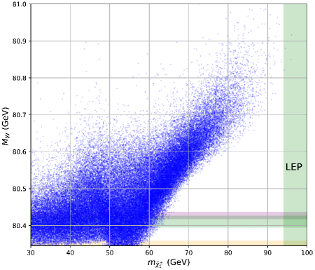
Figure 1: W boson mass vs lightest chargino mass for points generated in the ‘MSSM without $\mu$-term.’ The horizontal bands show the SM, Tevatron and world average masses for the W boson mass; the vertical green band shows the LEP constraint on the lightest chargino.

3.3 W mass in the MDGSSM

In the minimal Dirac Gaugino extension of the Standard Model (MDGSSM) the most typical scenario is to assume that R-symmetry is broken only via a $B_{\mu}$ term, i.e. the Higgs sector is special. It is identical to the previous model except that we allow a $\mu$-term. This, however, makes all the difference: now the higgsino mass is not bounded from below, not requiring a large mixing with the winos; and further the enhancement to the Higgs mass is under control.

We perform a new MCMC scan with parameters allowed to vary within the ranges:

$$m_{DY}\in[100,700]\,\ \mathrm{GeV}, \quad m_{D2}\in[100,1200]\,\ \mathrm{GeV},\quad v_{S}\in[-50,50]\,\ \mathrm{GeV},\quad v_{T}\in[-5,5]\,\ \mathrm{GeV}$$

$$\mu\in[0,1000]\,\ \mathrm{GeV}, \quad B_{\mu}\in[10^{4},10^{6}]\,(\ \mathrm{GeV})^{2},$$

$$\quad\sqrt{2}\lambda_{T}\in[-1.5,1.5], \quad\lambda_{S}\in[-1.5,1.5],\quad\tan\beta\in[2,50].$$ (3.14)

We fix the octet scalar, and all squark and slepton soft masses via $m_{O}^{2}=m_{\tilde{q}}^{2}=m_{\tilde{l}}^{2}=10$ TeV², and fix the gluino mass to $3$ TeV. We choose a likelihood function to be a product of a gaussian in the Higgs mass with mean $125$ GeV and standard deviation $3$ GeV, a gaussian in the W mass with mean $80.413$ GeV and standard deviation $20$ MeV, and a sigmoid on the constraints (given as the maximum ratio of predicted cross-section to observed, across all channels) from HiggsBounds5 [97, 98, 99, 100], which strongly suppresses the likelihood when the observed cross-section ratio is greater than one, but is otherwise close to unity. This choice of likelihood function is merely a device to select desirable points, and the distribution of the points is not meant to have a statistical interpretation in terms of their Bayesian likelihood; in particular, the theory uncertainty on the Higgs mass does not have a statistical interpretation, and a window of $3$ GeV is a conservative estimate of the average error, since we use the latest two-loop corrections in the generalised effective potential and gaugeless limit [101, 60, 102, 103] with pole-mass matching onto the SM [104] (see [105] for a recent review). Such a conservative window of $3$ GeV is employed because only a relatively small proportion of points actually generate a spectrum, and in principle a two-stage procedure pre-filtering points along those suggested in [64, 106] would probably be more efficient – or in addition the ability to invert the vacuum minimisation relations and compute $v_{S},v_{T}$ instead of treating them as inputs, but this is not yet automatically possible in the code in a way that would correctly incorporate the loop corrections to the Higgs masses [91].

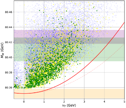
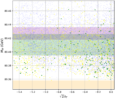
Figure 2: Left: W boson mass vs $v_{T}$ in the MDGSSM, with the red curve showing the tree-level prediction. Right: W boson mass vs $\sqrt{2}\lambda_{T}$ in the MDGSSM. Colours of the points are described in the text, with those obeying the strictest cuts shown in green. The colourful horizontal bands show the SM range in light orange; the Tevatron+LEP average in purple, and a conservative world average in green.

	MDG1	MDG2	MDG3
$m_{DY}$  (GeV)	280	285	245
$m_{D2}$  (GeV)	983	941	940
$\mu$  (GeV)	276	255	353
$\tan\beta$	48	46	47
$-\lambda_{S}$	1.179	1.074	1.112
$\sqrt{2}\lambda_{T}$	-0.487	0.502	0.099
$B_{\mu}$  $(\mathrm{GeV})^{2}$	828838	794477	938787
$v_{S}$  (GeV)	5.0	4.3	1.4
$v_{T}$  (GeV)	2.3	2.7	2.8
$m_{h_{1}}$  (GeV)	125.4	124.7	124.7
$m_{h_{2}}$  (GeV)	3120.9	2274.3	2405.8
$m_{A_{1}}$  (GeV)	2394.2	1221.4	1456.5
$m_{H_{1}^{\pm}}$  (GeV)	2400.2	1213.0	1455.3
$m_{\tilde{\chi}_{1}^{0}}$  (GeV)	217.9	231.5	233.0
$m_{\tilde{\chi}_{1}^{\pm}}$  (GeV)	255.0	275.9	362.0
$m_{W}$  (GeV)	80.425	80.420	80.421

Table 1: Benchmark points for the MDGSSM. Input parameters are given above the double line, and masses of the most important particles below.

We show plots in figure 2 for $M_{W}$ against $v_{T}$ (left plot), and then for $M_{W}$ against $\lambda_{T}$ (right plot), to show the points that benefit from large quantum corrections as the means of enhancing the $W$ mass: the tree-level expectation just from modifying $v_{T}$ is shown as a solid red curve on the left plot. We also show as a dashed red curve the value of $M_{W}$ that would be obtained by insisting that the shift in $\Delta\rho$ only modifies $M_{W}$ without changing $\sin\theta_{W}$ (if a different method of matching onto the SM parameters were used, for example).

All points shown satisfy all Higgs bounds; have a charged Higgs heavier than $600$ GeV (so are safe from $B\rightarrow s\gamma$ constraints [1]); have charginos heavier than the LEP limit and winos heavier than $600$ GeV. These baseline selections are marked as blue points in the plots; there are about 36000, of which about 10000 have $|v_{T}|<1$ GeV. Points shown in yellow further have charginos heavier than $200$ GeV, $m_{D2}>700$ GeV; while those marked in green have charginos heavier than $250$ GeV and $m_{D2}>800$ GeV (about $1600$ points in our sample survive these cuts). The green points are thus almost certainly guaranteed to be safe from current collider bounds (although they may yet be probed in future). The requirement of heavy charged Higgs scalars sets the MSSM-like neutral and pseudoscalar masses to be heavy, and essentially guarantees the safety of all selected points from constraints on the couplings of the SM-like Higgs. Nevertheless, we also filtered the green points with constraints from HiggsSignals [107, 108]. The different categories of points show the expected wider range of enhancements to the W mass as the charginos become lighter. We provide a selection of benchmark points, with the input parameters and crucial data, in table 1.

The first clear observation is that the quantum corrections to the W mass are at least as important as the tree-level contribution from the expectation value $v_{T}$, and the generic contribution to the W mass is positive with no points below the red curve. The asymmetry of the plot with $v_{T}$ is due to the fact that we only take positive Dirac gaugino masses. It is important to note that in the red curves we take the SM value of the W boson mass to be $80.352$ GeV, whereas the fitting function of [75] as employed in SARAH gives a value of $80.354$ GeV for the central values; and gives $80.356$ for a Higgs mass at the lower bound of our permitted range of $122$ GeV. However, it is clear that the quantum corrections in our sample are generally more important than $\Delta\rho_{\rm tree}$. Indeed, with the parameter ranges we have chosen, we are not within the range of masses required for decoupling of the quantum corrections (we have checked that the quantum corrections to $M_{W}$ smoothly drop to near zero as the masses of all particles are raised to about $2$ TeV or higher).

The second observation is that there is no clear correlation between the $W$ mass and the parameter $\lambda_{T}$. Due to our requirement of a large wino mass, the selected points have light neutralinos/charginos of mixed bino/higgsino type. The mass splitings among the higgsinos – and thus the contribution to the $W$ mass – can be driven large by $\lambda_{S}$ and $\lambda_{T}$. These couplings also enhance the Higgs mass at tree-level, so large values are favoured in the scans because we fixed the stop masses at $\sqrt{10}$ TeV. In this class of model there is therefore no particular preference for one or the other coupling.

Since the selected points generally have a mixed bino/higgsino LSP, they have good dark matter candidates, but it is expected that the relic density should be underdense. A detailed investigation of the dark matter-collider complementarity for scenarios satisfying the latest W mass data along the lines of [64] would be an interesting subject for future work, provided that the latest LHC analyses can be recast. As mentioned above, the possibility of a large $\lambda_{T}$ (and the presence of the singlet scalar/fermion) distinguishes higgsinos in this scenario from those in the MSSM. It is clear that this class of models provides a very natural explanation for an enhancement to the W mass compared to the Standard Model.

3.4 W mass in the aligned MDGSSM

In the aligned MDGSSM (where the only source of R-symmetry breaking is the $B_{\mu}$ term, and we take $T_{T}=0$), we choose the parameters to induce alignment at tree-level in the MDGSSM (so $\lambda_{S}=g_{Y}/\sqrt{2},\lambda_{T}=g_{2}/\sqrt{2}$ and $m_{DY}=c_{2\beta}\mu_{\rm eff}$ ) but taking $T_{S}=0$ (which means the mixing of the singlet with the heavy Higgs cannot vanish unless it is heavy). To study this scenario we perform a scan with the same strategy as before except that now, since $\lambda_{S},\lambda_{T}$ are fixed, it is necessary to vary the masses of the stops/sbottoms to allow us to find the observed value of the Higgs mass; there is also therefore a preference for models with larger $\tan\beta$ since the tree-level contributions to the Higgs mass at low $\tan\beta$ are not sufficient. We therefore use a common mass for the third generation squarks $M_{\rm SUSY};$ we set $m_{Q,33}^{2}=m_{U,33}^{2}=m_{D,33}^{2}=M_{\rm SUSY}^{2}$ (the other squarks and sleptons we retain fixed at $\sqrt{10}$ TeV). The remaining parameters are scanned via the same MCMC algorithm in the ranges:

$$m_{D2}\in[400,1500]\,\ \mathrm{GeV}, \quad v_{S}\in[-250,250]\,\ \mathrm{GeV},\quad v_{T}\in[-5,5]\,\ \mathrm{GeV}$$

$$\mu\in[-1000,1000]\,\ \mathrm{GeV}, \quad B_{\mu}\in[10^{4},10^{6}]\,(\ \mathrm{GeV})^{2},$$

$$M_{\rm SUSY}\in[2,10]\,\mathrm{TeV}, \quad\tan\beta\in[2,50].$$ (3.15)

We mostly find points with small $\mu/m_{DY}$ and very little enhancement to the W mass because the electroweakinos tend to be light. We give benchmark points in table 2 and plots in figure 3 which demonstrate the lack of enhancement and scarcity of points (790 survived from a scan for one million).

	AMDG1	AMDG2	AMDG3	AMDG4	AMDG5	AMDG6
$M_{\rm SUSY}$  (GeV)	8636.2	4550.9	5181.9	8436.1	7357.2	5454.9
$m_{D2}$  (GeV)	1037	1249	1149	1107	1219	994
$\tan\beta$	2	2	3	10	3	2
$\mu$  (GeV)	158.2	160.4	165.8	174.1	159.5	201.6
$v_{S}$  (GeV)	-19.0	-12.7	-8.4	-0.3	-5.0	-13.7
$v_{T}$  (GeV)	1.5	1.5	1.1	0.3	1.9	1.1
$m_{h_{1}}$  (GeV)	126.6	122.8	123.2	123.6	127.4	122.2
$m_{h_{2}}$  (GeV)	457.7	312.3	308.5	421.8	465.8	487.5
$m_{h_{3}}$  (GeV)	1282.2	799.7	935.2	1251.6	1176.5	762.3
$m_{h_{4}}$  (GeV)	2667.0	2965.0	3350.8	7104.7	2847.1	2933.0
$m_{H_{1}^{\pm}}$  (GeV)	1284.0	793.5	933.4	1257.7	1174.3	765.4
$m_{\tilde{\chi}_{1}^{0}}$  (GeV)	106.3	110.4	120.5	172.6	128.0	134.5
$m_{\tilde{\chi}_{1}^{\pm}}$  (GeV)	168.4	169.6	177.3	193.1	173.1	211.5
$m_{W}$  (GeV)	80.363	80.365	80.362	80.361	80.369	80.362

Table 2: Benchmark points with a light singlet in the Aligned MDGSSM

.

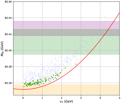
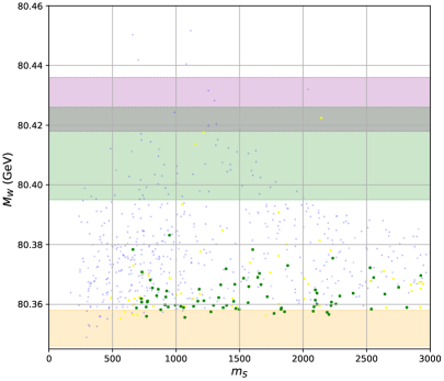
Figure 3: Points in the aligned MDGSSM. Left: $M_{W}$ against triplet expectation value. Right: $M_{W}$ against singlet-like scalar mass. Colour coding as for previous plots.

3.5 W mass in the aligned DGNMSSM

We turn now to the case of the aligned DGNMSSM described in section 2.4. We set the couplings $\lambda_{S},\lambda_{T}$ to their $N=2$ values and then choose $m_{DY}$ and $T_{S}$ to make $\Delta_{hs}$ and $\Delta_{Hs}$ vanish. This leads to

$$m_{DY}= c_{2\beta}\mu_{\rm eff}$$

$$T_{S}= -g_{Y}(\kappa v_{S}-\sqrt{2}s_{2\beta}\mu_{\rm eff}).$$ (3.16)

This has an interesting consequence because in this model

$$B_{\mu,\,\mathrm{eff}}= \frac{1}{\sqrt{2}}T_{S}v_{S}+\frac{1}{2}\lambda_{S}\kappa v_{S}^{2}=-\frac{1}{2\sqrt{2}}g_{Y}\kappa v_{S}^{2}+g_{Y}s_{2\beta}v_{S}\mu_{\rm eff}.$$ (3.17)

Then

$$M_{A}^{2}= g_{Y}v_{S}(2\mu_{\rm eff}-\frac{\kappa v_{S}}{\sqrt{2}s_{2\beta}})=g_{Y}v_{S}^{2}(g_{Y}-\frac{\kappa}{\sqrt{2}s_{2\beta}}).$$ (3.18)

We perform a scan using the same strategy as the previous sections; we use a common mass for the third generation squarks $M_{\rm SUSY};$ we set $m_{Q,33}^{2}=m_{U,33}^{2}=m_{D,33}^{2}=M_{\rm SUSY}^{2}$ (the other squarks and sleptons we retain fixed at $\sqrt{10}$ TeV). Then we scan with the parameter ranges, using the same likelihood function as before:

$$M_{\rm SUSY}\in[2000,10000] \,\ \mathrm{GeV},$$

$$\quad m_{D2}\in[400,1500] \,\ \mathrm{GeV},\quad v_{S}\in[-1500,1500]\,\ \mathrm{GeV},\quad v_{T}\in[-5,5]\,\ \mathrm{GeV}$$

$$\quad\kappa\in[-1.5,1.5], \quad T_{\kappa}\in[-2000,2000]\,\ \mathrm{GeV},\quad\tan\beta\in[2,50].$$ (3.19)

In our scans we impose that all Higgs searches are satisfied using HiggsBounds and HiggsSignals. We show the results for the W boson mass in figure 4 where the points have the same colour coding as in the previous sections. It is apparent that in this model it is complicated to enhance the W boson mass. This is because we have only a small quantum effect from $\lambda_{S},\lambda_{T}$, but also because the lightest neutralinos are typically rather light: since $\mu_{\rm eff}=g_{Y}v_{S}/2$ we need a large $v_{S}\gtrsim 500$ GeV (or $1$ TeV for our more stringent points) to have heavy enough higgsinos. Then we need $\kappa$ negative and not too small to avoid a too-small pseudoscalar/charged Higgs mass (if we neglect $\kappa$ then $M_{A}$ is bounded by $g_{Y}v_{S}$, so $M_{A}>600$ GeV requires $v_{S}\gtrsim 1700$ GeV, at the limit of our search range). So this implies that the singlino is generally heavy compared to $m_{DY}$:

$$\frac{m_{DY}}{\sqrt{2}\kappa v_{S}}= \frac{g_{Y}c_{2\beta}}{2\sqrt{2}\kappa}.$$ (3.20)

In figure 4 we show the scan results with the same colour coding as in previous sections. It is clear that in this scenario, models which can explain a large $W$ mass are driven by a larger $v_{T}$ with some modest quantum corrections enhancing the mass by $\mathcal{O}(10)$ MeV; there is very little spread due to the lack of variation in $\lambda_{T}$. However, it is difficult to find points with large enough $v_{T}$ that satisfy other bounds.

Another feature of the selected points is that in almost all cases $v_{T}>0$; considering $T_{T}=M_{T}=0$ in equation (2.18) means that in order for $\tilde{m}_{TR}^{2}>0$ (so that, at least, the pseudoscalar triplet should be non-tachyonic, since we take $B_{T}=0$) and $v_{T}<0$ we would need $\mu_{\rm eff}>|m_{D2}c_{2\beta}|$. But we need large $\tan\beta$ to obtain the correct Higgs mass, and therefore $g_{Y}v_{S}/2\gtrsim m_{D2}$; for our selected points we require a minimum of $m_{D2}>600$ GeV, and so $v_{S}$ would again be beyond our search range.

Since we are interested here in alignment, we may have a light singlet scalar without falling foul of either light Higgs or heavy Higgs searches. In this limit we have

$$\tilde{m}_{S}^{2}\rightarrow \frac{1}{4}\bigg{[}2v_{S}(\sqrt{2}T_{\kappa}+3\sqrt{2}\kappa M_{S}+4v_{S}\kappa^{2})+v^{2}g_{Y}(g_{Y}-\sqrt{2}\kappa s_{2\beta})\bigg{]}.$$ (3.21)

$T_{\kappa}$ of opposite sign to $v_{S}$ allows the singlet to be made light while making $M_{A}$ arbitrarily heavy. In the scan, we do not impose any likelihood bias to search for points with a light singlet, but we show benchmark points passing all constraints which have light singlet masses in table 3. They show a W mass consistent with the SM prediction.

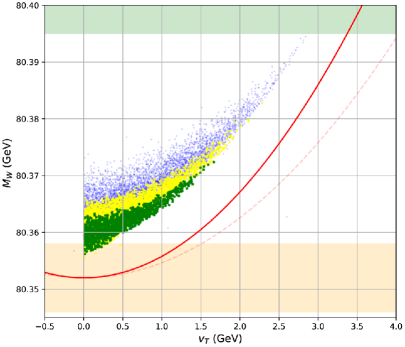
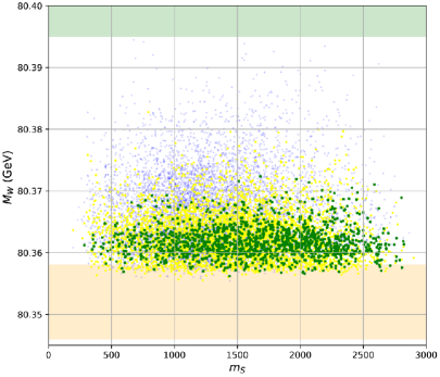
Figure 4: W boson mass in the aligned DGNMSSM. Left: W boson mass against triplet expectation value. Right: W boson mass against singlet-like Higgs mass. Colour coding of points is described in the text.

	A-DGN1	A-DGN2	A-DGN3	A-DGN4
$M_{\rm SUSY}$  (GeV)	6368.4	5186.5	8219.5	8702.9
$m_{D2}$  (GeV)	802	991	932	923
$\tan\beta$	26	11	29	22
$\kappa$	-0.418	-0.332	-0.446	-0.418
$v_{S}$  (GeV)	1417.4	1402.4	1337.0	1488.8
$v_{T}$  (GeV)	0.2	0.1	0.1	0.8
$T_{\kappa}$  (GeV)	-595.6	-267.5	-648.0	-639.4
$m_{h_{1}}$  (GeV)	124.1	122.9	125.2	123.4
$m_{h_{2}}$  (GeV)	353.5	417.6	347.2	353.9
$m_{h_{3}}$  (GeV)	1838.5	1284.5	1843.0	1803.0
$m_{h_{4}}$  (GeV)	6710.7	12226.0	10817.9	4056.2
$m_{H_{1}^{\pm}}$  (GeV)	1841.4	1288.5	1846.1	1806.2
$m_{\tilde{\chi}_{1}^{0}}$  (GeV)	72.2	84.2	64.5	75.2
$m_{\tilde{\chi}_{1}^{\pm}}$  (GeV)	280.1	274.6	265.1	291.9
$m_{W}$  (GeV)	80.362	80.361	80.361	80.363

Table 3: Benchmark points for the “aligned DGNMSSM”. Input parameters are given above the double line, and masses of the most important particles below.

3.6 W mass in the general DGNMSSM

Finally we consider the general DGNMSSM, where we allow the values of $\lambda_{S},\lambda_{T}$ to vary and do not fix the values of $m_{DY}$ or $T_{S}$ to require alignment but scan over them. This means that we will not focus on light singlet (or doublet) scalars. Similar to the aligned case, there is still a see-saw effect on the lightest neutralino mass due to the non-zero singlino mass, which can drive down the quantum corrections to the W boson, but a large $|\lambda_{T}|$ can compensate for this and also help enhance the SM-like Higgs mass.

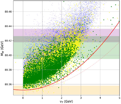
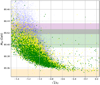
Figure 5: W boson mass in the general DGNMSSM. Left: W boson mass against triplet expectation value. Right: W boson mass against $\lambda_{T}$. Colour coding of points as in previous figures.

	DGN1	DGN2	DGN3	DGN4	DGN5
$m_{DY}$  (GeV)	392	298	410	380	292
$m_{D2}$  (GeV)	927	971	841	1003	805
$\kappa$	1.391	-1.369	-1.266	-1.309	-1.361
$\tan\beta$	9	23	21	30	30
$-\lambda_{S}$	0.727	-0.893	-0.544	0.554	-0.677
$\sqrt{2}\lambda_{T}$	-1.426	1.496	1.463	-1.303	-1.296
$-T_{S}$  $(\ \mathrm{GeV})$	3077	3747	-2496	-3002	1183
$T_{\kappa}$  $(\ \mathrm{GeV})$	1139	350	-1292	-571	728
$v_{S}$  (GeV)	-658.1	-539.1	574.5	524.7	-482.8
$v_{T}$  (GeV)	2.7	2.3	1.7	2.5	2.2
$m_{h_{1}}$  (GeV)	125.1	125.3	125.8	124.6	124.7
$m_{h_{2}}$  (GeV)	1017.6	937.1	665.0	831.8	740.1
$m_{A_{1}}$  (GeV)	757.6	93.7	778.1	115.1	502.2
$m_{H_{1}^{\pm}}$  (GeV)	2793.1	3195.1	1281.7	778.5	806.5
$m_{\tilde{\chi}_{1}^{0}}$  (GeV)	115.0	87.2	123.6	110.9	90.7
$m_{\tilde{\chi}_{1}^{\pm}}$  (GeV)	278.8	273.6	265.5	254.8	268.8
$m_{W}$  (GeV)	80.421	80.421	80.424	80.420	80.422

Table 4: Benchmark points for the general DGNSSM. Input parameters are given above the double line, and masses of the most important particles below.

We perform a scan using the strategy as in sections 3.2 and 3.3, with the parameter ranges:

$$m_{DY}\in[100,700]\,\ \mathrm{GeV}, \quad m_{D2}\in[150,1200]\,\ \mathrm{GeV},\quad v_{S}\in[-700,700]\,\ \mathrm{GeV},\quad v_{T}\in[-5,5]\,\ \mathrm{GeV}$$

$$\qquad\kappa\in[-1.5,1.5],\qquad T_{\kappa}\in[-2000,2000]\,\ \mathrm{GeV},\qquad T_{S}\in[-4000,4000]\,\ \mathrm{GeV},$$

$$\qquad\lambda_{S}\in[-1.5,1.5], \qquad\sqrt{2}\lambda_{T}\in[-1.5,1.5],\qquad\tan\beta\in[2,50].$$ (3.22)

We give plots in figure 5 with the same colour coding as in the previous sections; the difference in the distribution to the previous examples is rather striking. It is clear that in this scenario a large negative $\lambda_{T}$ and a positive $v_{T}$ is favoured; this gives a tree-level enhancement to the Higgs mass and a loop-level enhancement to the $W$-boson mass. The singlino component will mix less with the higgsinos than in the MDGSSM because of the $\sqrt{2}\kappa v_{S}$ singlino mass, and thus the effect of $\lambda_{S}$ on the $W$ mass is diminished. The asymmetry in the signs of $\lambda_{T}$ and $v_{T}$ can be explained by the fact that we only take positive Dirac gaugino masses in the scans.

4 Conclusions

We have shown that an aligned Dirac Gaugino NMSSM is possible and compatible with current collider constraints; it can even lead to relatively light singlet scalars that may be of interest to future searches (although would be rather difficult to find directly as they are difficult to produce). Such a model favours a W boson mass compatible with or just above the SM prediction. We also showed how two different Dirac Gaugino scenarios can easily be compatible with an enhanced W boson mass, including a precise computation of the quantum corrections for the first time, which are now incorporated automatically in the package SARAH. We also used this computation to add more nails to the coffin of the “MSSM without $\mu$ term.”

We have been conservative in our application of collider constraints and concluded that the MDGSSM models would typically contain underdense dark matter densities. However, it would be interesting to examine the issue of dark matter and collider constraints again in all of these classes of models when all the latest searches for electroweakinos have been recast; we have provided ample benchmark points for this purpose. In the DGNMSSM or its aligned version, if we impose strict R-parity or have a heavy gravitino (by no means entirely obvious assumptions), it may be that we require a Higgs funnel to obtain the correct relic density, which would require a sophisticated search strategy to find allowed parameter ranges, along e.g. the lines of [106]. However, it is also likely that a light singlino in the aligned DGNMSSM could fulfil the role of the Higgs funnel. We leave these questions to future work.

References

- [1] M. Misiak and M. Steinhauser, Weak radiative decays of the B meson and bounds on in the Two-Higgs-Doublet Model. Eur. Phys. J. C77 (2017) no. 3, 201, arXiv:1702.04571 [hep-ph].
- [2] S. Davidson and H. E. Haber, Basis-independent methods for the two-Higgs-doublet model. Phys. Rev. D 72 (2005) 035004, arXiv:hep-ph/0504050. [Erratum: Phys.Rev.D 72, 099902 (2005)].
- [3] P. S. Bhupal Dev and A. Pilaftsis, Maximally Symmetric Two Higgs Doublet Model with Natural Standard Model Alignment. JHEP 12 (2014) 024, arXiv:1408.3405 [hep-ph]. [Erratum: JHEP 11, 147 (2015)].
- [4] J. Bernon, J. F. Gunion, H. E. Haber, Y. Jiang, and S. Kraml, Scrutinizing the alignment limit in two-Higgs-doublet models: mh=125 GeV. Phys. Rev. D 92 (2015) no. 7, 075004, arXiv:1507.00933 [hep-ph].
- [5] J. Bernon, J. F. Gunion, H. E. Haber, Y. Jiang, and S. Kraml, Scrutinizing the alignment limit in two-Higgs-doublet models. II. mH=125 GeV. Phys. Rev. D 93 (2016) no. 3, 035027, arXiv:1511.03682 [hep-ph].
- [6] M. Carena, I. Low, N. R. Shah, and C. E. M. Wagner, Impersonating the Standard Model Higgs Boson: Alignment without Decoupling. JHEP 04 (2014) 015, arXiv:1310.2248 [hep-ph].
- [7] M. Carena, H. E. Haber, I. Low, N. R. Shah, and C. E. M. Wagner, Alignment limit of the NMSSM Higgs sector. Phys. Rev. D93 (2016) no. 3, 035013, arXiv:1510.09137 [hep-ph].
- [8] H. E. Haber, S. Heinemeyer, and T. Stefaniak, The Impact of Two-Loop Effects on the Scenario of MSSM Higgs Alignment without Decoupling. Eur. Phys. J. C 77 (2017) no. 11, 742, arXiv:1708.04416 [hep-ph].
- [9] N. M. Coyle and C. E. M. Wagner, Dynamical Higgs field alignment in the NMSSM. Phys. Rev. D 101 (2020) no. 5, 055037, arXiv:1912.01036 [hep-ph].
- [10] P. Fayet, MASSIVE GLUINOS. Phys. Lett. B 78 (1978) 417–420.
- [11] J. Polchinski and L. Susskind, Breaking of Supersymmetry at Intermediate-Energy. Phys. Rev. D26 (1982) 3661.
- [12] L. J. Hall and L. Randall, U(1)-R symmetric supersymmetry. Nucl. Phys. B352 (1991) 289–308.
- [13] P. J. Fox, A. E. Nelson, and N. Weiner, Dirac gaugino masses and supersoft supersymmetry breaking. JHEP 08 (2002) 035, arXiv:hep-ph/0206096.
- [14] A. E. Nelson, N. Rius, V. Sanz, and M. Unsal, The Minimal supersymmetric model without a mu term. JHEP 08 (2002) 039, arXiv:hep-ph/0206102.
- [15] I. Antoniadis, K. Benakli, A. Delgado, and M. Quiros, A New gauge mediation theory. Adv. Stud. Theor. Phys. 2 (2008) 645–672, arXiv:hep-ph/0610265.
- [16] G. Belanger, K. Benakli, M. Goodsell, C. Moura, and A. Pukhov, Dark Matter with Dirac and Majorana Gaugino Masses. JCAP 08 (2009) 027, arXiv:0905.1043 [hep-ph].
- [17] K. Benakli and M. D. Goodsell, Dirac Gauginos in General Gauge Mediation. Nucl. Phys. B 816 (2009) 185–203, arXiv:0811.4409 [hep-ph].
- [18] K. Benakli, M. D. Goodsell, and A.-K. Maier, Generating mu and Bmu in models with Dirac Gauginos. Nucl. Phys. B851 (2011) 445–461, arXiv:1104.2695 [hep-ph].
- [19] G. D. Kribs, E. Poppitz, and N. Weiner, Flavor in supersymmetry with an extended R-symmetry. Phys. Rev. D78 (2008) 055010, arXiv:0712.2039 [hep-ph].
- [20] S. D. L. Amigo, A. E. Blechman, P. J. Fox, and E. Poppitz, R-symmetric gauge mediation. JHEP 01 (2009) 018, arXiv:0809.1112 [hep-ph].
- [21] K. Benakli and M. D. Goodsell, Dirac Gauginos and Kinetic Mixing. Nucl. Phys. B 830 (2010) 315–329, arXiv:0909.0017 [hep-ph].
- [22] S. Y. Choi, J. Kalinowski, J. M. Kim, and E. Popenda, Scalar gluons and Dirac gluinos at the LHC. Acta Phys. Polon. B40 (2009) 2913–2922, arXiv:0911.1951 [hep-ph].
- [23] K. Benakli and M. D. Goodsell, Dirac Gauginos, Gauge Mediation and Unification. Nucl. Phys. B 840 (2010) 1–28, arXiv:1003.4957 [hep-ph].
- [24] S. Y. Choi, D. Choudhury, A. Freitas, J. Kalinowski, J. M. Kim, and P. M. Zerwas, Dirac Neutralinos and Electroweak Scalar Bosons of N=1/N=2 Hybrid Supersymmetry at Colliders. JHEP 08 (2010) 025, arXiv:1005.0818 [hep-ph].
- [25] L. M. Carpenter, Dirac Gauginos, Negative Supertraces and Gauge Mediation. JHEP 09 (2012) 102, arXiv:1007.0017 [hep-th].
- [26] S. Abel and M. Goodsell, Easy Dirac Gauginos. JHEP 06 (2011) 064, arXiv:1102.0014 [hep-th].
- [27] R. Davies, J. March-Russell, and M. McCullough, A Supersymmetric One Higgs Doublet Model. JHEP 04 (2011) 108, arXiv:1103.1647 [hep-ph].
- [28] K. Benakli, Dirac Gauginos: A User Manual. Fortsch. Phys. 59 (2011) 1079–1082, arXiv:1106.1649 [hep-ph].
- [29] C. Frugiuele and T. Gregoire, Making the Sneutrino a Higgs with a Lepton Number. Phys. Rev. D85 (2012) 015016, arXiv:1107.4634 [hep-ph].
- [30] H. Itoyama and N. Maru, D-term Dynamical Supersymmetry Breaking Generating Split N=2 Gaugino Masses of Mixed Majorana-Dirac Type. Int. J. Mod. Phys. A27 (2012) 1250159, arXiv:1109.2276 [hep-ph].
- [31] E. Bertuzzo and C. Frugiuele, Fitting Neutrino Physics with a Lepton Number. JHEP 05 (2012) 100, arXiv:1203.5340 [hep-ph].
- [32] R. Davies, Dirac gauginos and unification in F-theory. JHEP 10 (2012) 010, arXiv:1205.1942 [hep-th].
- [33] C. Frugiuele, T. Gregoire, P. Kumar, and E. Ponton, ’L=R’ - as the Origin of Leptonic ’RPV’. JHEP 03 (2013) 156, arXiv:1210.0541 [hep-ph].
- [34] C. Frugiuele, T. Gregoire, P. Kumar, and E. Ponton, ’L=R’ – Lepton Number at the LHC. JHEP 05 (2013) 012, arXiv:1210.5257 [hep-ph].
- [35] K. Benakli, M. D. Goodsell, and F. Staub, Dirac Gauginos and the 125 GeV Higgs. JHEP 06 (2013) 073, arXiv:1211.0552 [hep-ph].
- [36] E. Dudas, M. Goodsell, L. Heurtier, and P. Tziveloglou, Flavour models with Dirac and fake gluinos. Nucl. Phys. B884 (2014) 632–671, arXiv:1312.2011 [hep-ph].
- [37] K. Benakli, L. Darmé, M. D. Goodsell, and P. Slavich, A Fake Split Supersymmetry Model for the 126 GeV Higgs. JHEP 05 (2014) 113, arXiv:1312.5220 [hep-ph].
- [38] K. Benakli, L. Darmé, and M. D. Goodsell, (O)Mega Split. JHEP 11 (2015) 100, arXiv:1508.02534 [hep-ph].
- [39] A. Arvanitaki, M. Baryakhtar, X. Huang, K. van Tilburg, and G. Villadoro, The Last Vestiges of Naturalness. JHEP 03 (2014) 022, arXiv:1309.3568 [hep-ph].
- [40] H. Itoyama and N. Maru, D-term Triggered Dynamical Supersymmetry Breaking. Phys. Rev. D88 (2013) no. 2, 025012, arXiv:1301.7548 [hep-ph].
- [41] S. Chakraborty and S. Roy, Higgs boson mass, neutrino masses and mixing and keV dark matter in an lepton number model. JHEP 01 (2014) 101, arXiv:1309.6538 [hep-ph].
- [42] C. Csaki, J. Goodman, R. Pavesi, and Y. Shirman, The problem of Dirac gauginos and its solutions. Phys. Rev. D89 (2014) no. 5, 055005, arXiv:1310.4504 [hep-ph].
- [43] H. Itoyama and N. Maru, 126 GeV Higgs Boson Associated with D-term Triggered Dynamical Supersymmetry Breaking. Symmetry 7 (2015) no. 1, 193–205, arXiv:1312.4157 [hep-ph].
- [44] H. Beauchesne and T. Gregoire, Electroweak precision measurements in supersymmetric models with a U(1)R lepton number. JHEP 05 (2014) 051, arXiv:1402.5403 [hep-ph].
- [45] K. Benakli, (Pseudo)goldstinos, SUSY fluids, Dirac gravitino and gauginos. EPJ Web Conf. 71 (2014) 00012, arXiv:1402.4286 [hep-ph].
- [46] E. Bertuzzo, C. Frugiuele, T. Gregoire, and E. Ponton, Dirac gauginos, R symmetry and the 125 GeV Higgs. JHEP 04 (2015) 089, arXiv:1402.5432 [hep-ph].
- [47] P. Dießner, J. Kalinowski, W. Kotlarski, and D. Stöckinger, Higgs boson mass and electroweak observables in the MRSSM. JHEP 12 (2014) 124, arXiv:1410.4791 [hep-ph].
- [48] K. Benakli, M. Goodsell, F. Staub, and W. Porod, Constrained minimal Dirac gaugino supersymmetric standard model. Phys. Rev. D 90 (2014) no. 4, 045017, arXiv:1403.5122 [hep-ph].
- [49] M. D. Goodsell and P. Tziveloglou, Dirac Gauginos in Low Scale Supersymmetry Breaking. Nucl. Phys. B889 (2014) 650–675, arXiv:1407.5076 [hep-ph].
- [50] D. Busbridge, Constrained Dirac gluino mediation. arXiv:1408.4605 [hep-ph].
- [51] S. Chakraborty, A. Datta, and S. Roy, in U(1)R -lepton number model with a right-handed neutrino. JHEP 02 (2015) 124, arXiv:1411.1525 [hep-ph]. [Erratum: JHEP09,077(2015)].
- [52] R. Ding, T. Li, F. Staub, C. Tian, and B. Zhu, Supersymmetric standard models with a pseudo-Dirac gluino from hybrid F - and D -term supersymmetry breaking. Phys. Rev. D92 (2015) no. 1, 015008, arXiv:1502.03614 [hep-ph].
- [53] D. S. M. Alves, J. Galloway, M. McCullough, and N. Weiner, Goldstone Gauginos. Phys. Rev. Lett. 115 (2015) no. 16, 161801, arXiv:1502.03819 [hep-ph].
- [54] D. S. M. Alves, J. Galloway, M. McCullough, and N. Weiner, Models of Goldstone Gauginos. Phys. Rev. D93 (2016) no. 7, 075021, arXiv:1502.05055 [hep-ph].
- [55] L. M. Carpenter and J. Goodman, New Calculations in Dirac Gaugino Models: Operators, Expansions, and Effects. JHEP 07 (2015) 107, arXiv:1501.05653 [hep-ph].
- [56] S. P. Martin, Nonstandard supersymmetry breaking and Dirac gaugino masses without supersoftness. Phys. Rev. D92 (2015) no. 3, 035004, arXiv:1506.02105 [hep-ph].
- [57] M. D. Goodsell, M. E. Krauss, T. Müller, W. Porod, and F. Staub, Dark matter scenarios in a constrained model with Dirac gauginos. JHEP 10 (2015) 132, arXiv:1507.01010 [hep-ph].
- [58] W. Kotlarski, Sgluons in the same-sign lepton searches. JHEP 02 (2017) 027, arXiv:1608.00915 [hep-ph].
- [59] K. Benakli, L. Darmé, M. D. Goodsell, and J. Harz, The Di-Photon Excess in a Perturbative SUSY Model. Nucl. Phys. B911 (2016) 127–162, arXiv:1605.05313 [hep-ph].
- [60] J. Braathen, M. D. Goodsell, and P. Slavich, Leading two-loop corrections to the Higgs boson masses in SUSY models with Dirac gauginos. JHEP 09 (2016) 045, arXiv:1606.09213 [hep-ph].
- [61] S. Chakraborty and J. Chakrabortty, Natural emergence of neutrino masses and dark matter from -symmetry. JHEP 10 (2017) 012, arXiv:1701.04566 [hep-ph].
- [62] G. Chalons, M. D. Goodsell, S. Kraml, H. Reyes-González, and S. L. Williamson, LHC limits on gluinos and squarks in the minimal Dirac gaugino model. JHEP 04 (2019) 113, arXiv:1812.09293 [hep-ph].
- [63] L. M. Carpenter, T. Murphy, and M. J. Smylie, Exploring color-octet scalar parameter space in minimal -symmetric models. JHEP 11 (2020) 024, arXiv:2006.15217 [hep-ph].
- [64] M. D. Goodsell, S. Kraml, H. Reyes-González, and S. L. Williamson, Constraining Electroweakinos in the Minimal Dirac Gaugino Model. SciPost Phys. 9 (2020) no. 4, 047, arXiv:2007.08498 [hep-ph].
- [65] L. M. Carpenter and T. Murphy, Color-octet scalars in Dirac gaugino models with broken symmetry. JHEP 05 (2021) 079, arXiv:2012.15771 [hep-ph].
- [66] K. Benakli, M. D. Goodsell, and S. L. Williamson, Higgs alignment from extended supersymmetry. Eur. Phys. J. C 78 (2018) no. 8, 658, arXiv:1801.08849 [hep-ph].
- [67] K. Benakli, Y. Chen, and G. Lafforgue-Marmet, R-symmetry for Higgs alignment without decoupling. Eur. Phys. J. C 79 (2019) no. 2, 172, arXiv:1811.08435 [hep-ph].
- [68] K. Benakli, Y. Chen, and G. Lafforgue-Marmet, Predicting Alignment in a Two Higgs Doublet Model. MDPI Proc. 13 (2019) no. 1, 2, arXiv:1812.02208 [hep-ph].
- [69] K. Benakli, Y. Chen, and G. Lafforgue-Marmet, An Emergent Higgs Alignment. PoS CORFU2018 (2019) 014, arXiv:1904.04248 [hep-ph].
- [70] J. Ellis, J. Quevillon, and V. Sanz, Doubling Up on Supersymmetry in the Higgs Sector. JHEP 10 (2016) 086, arXiv:1607.05541 [hep-ph].
- [71] CMS Collaboration, Combined Higgs boson production and decay measurements with up to 137 fb-1 of proton-proton collision data at = 13 TeV.
- [72] ATLAS Collaboration, A combination of measurements of Higgs boson production and decay using up to fb-1 of proton–proton collision data at 13 TeV collected with the ATLAS experiment.
- [73] CDF Collaboration, T. Aaltonen et al., High-precision measurement of the W boson mass with the CDF II detector. Science 376 (2022) no. 6589, 170–176.
- [74] M. Awramik, M. Czakon, A. Freitas, and G. Weiglein, Precise prediction for the W boson mass in the standard model. Phys. Rev. D 69 (2004) 053006, arXiv:hep-ph/0311148.
- [75] G. Degrassi, P. Gambino, and P. P. Giardino, The interdependence in the Standard Model: a new scrutiny. JHEP 05 (2015) 154, arXiv:1411.7040 [hep-ph].
- [76] OPAL Collaboration, G. Abbiendi et al., Measurement of the mass and width of the boson. Eur. Phys. J. C 45 (2006) 307–335, arXiv:hep-ex/0508060.
- [77] L3 Collaboration, P. Achard et al., Measurement of the mass and the width of the boson at LEP. Eur. Phys. J. C 45 (2006) 569–587, arXiv:hep-ex/0511049.
- [78] ALEPH Collaboration, S. Schael et al., Measurement of the boson mass and width in collisions at LEP. Eur. Phys. J. C 47 (2006) 309–335, arXiv:hep-ex/0605011.
- [79] DELPHI Collaboration, J. Abdallah et al., Measurement of the Mass and Width of the Boson in Collisions at = 161-GeV - 209-GeV. Eur. Phys. J. C 55 (2008) 1–38, arXiv:0803.2534 [hep-ex].
- [80] ALEPH, DELPHI, L3, OPAL, LEP Electroweak Collaboration, S. Schael et al., Electroweak Measurements in Electron-Positron Collisions at W-Boson-Pair Energies at LEP. Phys. Rept. 532 (2013) 119–244, arXiv:1302.3415 [hep-ex].
- [81] D0 Collaboration, V. M. Abazov et al., Measurement of the W Boson Mass with the D0 Detector. Phys. Rev. Lett. 108 (2012) 151804, arXiv:1203.0293 [hep-ex].
- [82] CDF Collaboration, T. Aaltonen et al., Precise measurement of the -boson mass with the CDF II detector. Phys. Rev. Lett. 108 (2012) 151803, arXiv:1203.0275 [hep-ex].
- [83] CDF, D0 Collaboration, T. A. Aaltonen et al., Combination of CDF and D0 -Boson Mass Measurements. Phys. Rev. D 88 (2013) no. 5, 052018, arXiv:1307.7627 [hep-ex].
- [84] S. Heinemeyer, W. Hollik, G. Weiglein, and L. Zeune, Implications of LHC search results on the W boson mass prediction in the MSSM. JHEP 12 (2013) 084, arXiv:1311.1663 [hep-ph].
- [85] ATLAS Collaboration, M. Aaboud et al., Measurement of the -boson mass in pp collisions at TeV with the ATLAS detector. Eur. Phys. J. C 78 (2018) no. 2, 110, arXiv:1701.07240 [hep-ex]. [Erratum: Eur.Phys.J.C 78, 898 (2018)].
- [86] LHCb Collaboration, R. Aaij et al., Measurement of the W boson mass. JHEP 01 (2022) 036, arXiv:2109.01113 [hep-ex].
- [87] P. Athron, M. Bach, D. H. J. Jacob, W. Kotlarski, D. Stöckinger, and A. Voigt, Precise calculation of the W boson pole mass beyond the Standard Model with FlexibleSUSY. arXiv:2204.05285 [hep-ph].
- [88] P. Athron, J.-h. Park, D. Stöckinger, and A. Voigt, FlexibleSUSY – a meta spectrum generator for supersymmetric models. Nucl. Part. Phys. Proc. 273-275 (2016) 2424–2426, arXiv:1410.7385 [hep-ph].
- [89] P. Athron, M. Bach, D. Harries, T. Kwasnitza, J.-h. Park, D. Stöckinger, A. Voigt, and J. Ziebell, FlexibleSUSY 2.0: Extensions to investigate the phenomenology of SUSY and non-SUSY models. Comput. Phys. Commun. 230 (2018) 145–217, arXiv:1710.03760 [hep-ph].
- [90] P. Diessner and G. Weiglein, Precise prediction for the W boson mass in the MRSSM. JHEP 07 (2019) 011, arXiv:1904.03634 [hep-ph].
- [91] J. Braathen, M. D. Goodsell, S. Paßehr, and E. Pinsard, Expectation management. Eur. Phys. J. C 81 (2021) no. 6, 498, arXiv:2103.06773 [hep-ph].
- [92] M. Carena, H. E. Haber, I. Low, N. R. Shah, and C. E. M. Wagner, Complementarity between Nonstandard Higgs Boson Searches and Precision Higgs Boson Measurements in the MSSM. Phys. Rev. D91 (2015) no. 3, 035003, arXiv:1410.4969 [hep-ph].
- [93] M. Du, Z. Liu, and P. Nath, CDF W mass anomaly from a dark sector with a Stueckelberg-Higgs portal. arXiv:2204.09024 [hep-ph].
- [94] ALEPH Collaboration, A. Heister et al., Search for charginos nearly mass degenerate with the lightest neutralino in e+ e- collisions at center-of-mass energies up to 209-GeV. Phys. Lett. B 533 (2002) 223–236, arXiv:hep-ex/0203020.
- [95] J. Abdallah et al., Searches for supersymmetric particles in e+e- collisions up to 208 GeV, and interpretation of the results within the MSSM.
- [96] LEP2 SUSY Working Group, ALEPH, DELPHI, L3 and OPAL experiments, note LEPSUSYWG/02-04.1. {http://lepsusy.web.cern.ch/lepsusy/Welcome.html}.
- [97] P. Bechtle, O. Brein, S. Heinemeyer, G. Weiglein, and K. E. Williams, HiggsBounds: Confronting Arbitrary Higgs Sectors with Exclusion Bounds from LEP and the Tevatron. Comput. Phys. Commun. 181 (2010) 138–167, arXiv:0811.4169 [hep-ph].
- [98] P. Bechtle, O. Brein, S. Heinemeyer, G. Weiglein, and K. E. Williams, HiggsBounds 2.0.0: Confronting Neutral and Charged Higgs Sector Predictions with Exclusion Bounds from LEP and the Tevatron. Comput. Phys. Commun. 182 (2011) 2605–2631, arXiv:1102.1898 [hep-ph].
- [99] P. Bechtle, O. Brein, S. Heinemeyer, O. Stål, T. Stefaniak, G. Weiglein, and K. E. Williams, : Improved Tests of Extended Higgs Sectors against Exclusion Bounds from LEP, the Tevatron and the LHC. Eur. Phys. J. C 74 (2014) no. 3, 2693, arXiv:1311.0055 [hep-ph].
- [100] P. Bechtle, D. Dercks, S. Heinemeyer, T. Klingl, T. Stefaniak, G. Weiglein, and J. Wittbrodt, HiggsBounds-5: Testing Higgs Sectors in the LHC 13 TeV Era. Eur. Phys. J. C 80 (2020) no. 12, 1211, arXiv:2006.06007 [hep-ph].
- [101] M. Goodsell, K. Nickel, and F. Staub, Generic two-loop Higgs mass calculation from a diagrammatic approach. Eur. Phys. J. C75 (2015) no. 6, 290, arXiv:1503.03098 [hep-ph].
- [102] J. Braathen and M. D. Goodsell, Avoiding the Goldstone Boson Catastrophe in general renormalisable field theories at two loops. JHEP 12 (2016) 056, arXiv:1609.06977 [hep-ph].
- [103] J. Braathen, M. D. Goodsell, and F. Staub, Supersymmetric and non-supersymmetric models without catastrophic Goldstone bosons. Eur. Phys. J. C77 (2017) no. 11, 757, arXiv:1706.05372 [hep-ph].
- [104] F. Staub and W. Porod, Improved predictions for intermediate and heavy Supersymmetry in the MSSM and beyond. Eur. Phys. J. C 77 (2017) no. 5, 338, arXiv:1703.03267 [hep-ph].
- [105] P. Slavich et al., Higgs-mass predictions in the MSSM and beyond. Eur. Phys. J. C 81 (2021) no. 5, 450, arXiv:2012.15629 [hep-ph].
- [106] M. D. Goodsell and A. Joury, Active learning BSM parameter spaces. arXiv:2204.13950 [hep-ph].
- [107] P. Bechtle, S. Heinemeyer, O. Stål, T. Stefaniak, and G. Weiglein, : Confronting arbitrary Higgs sectors with measurements at the Tevatron and the LHC. Eur. Phys. J. C 74 (2014) no. 2, 2711, arXiv:1305.1933 [hep-ph].
- [108] P. Bechtle, S. Heinemeyer, T. Klingl, T. Stefaniak, G. Weiglein, and J. Wittbrodt, HiggsSignals-2: Probing new physics with precision Higgs measurements in the LHC 13 TeV era. Eur. Phys. J. C 81 (2021) no. 2, 145, arXiv:2012.09197 [hep-ph].