MultiMatch: Multi-task Learning for Semi-supervised Domain Generalization

Abstract

Domain generalization (DG) aims at learning a model on source domains to well generalize on the unseen target domain. Although it has achieved a great success, most of existing methods require the label information for all training samples in source domains, which is time-consuming and expensive in the real-world application. In this paper, we resort to solving the semi-supervised domain generalization (SSDG) task, where there are a few label information in each source domain. To address the task, we first analyze the theory of the multi-domain learning, which highlights that 1) mitigating the impact of domain gap and 2) exploiting all samples to train the model can effectively reduce the generalization error in each source domain so as to improve the quality of pseudo-labels. According to the analysis, we propose MultiMatch, i.e., extending FixMatch to the multi-task learning framework, producing the high-quality pseudo-label for SSDG. To be specific, we consider each training domain as a single task (i.e., local task) and combine all training domains together (i.e., global task) to train an extra task for the unseen test domain. In the multi-task framework, we utilize the independent BN and classifier for each task, which can effectively alleviate the interference from different domains during pseudo-labeling. Also, most of parameters in the framework are shared, which can be trained by all training samples sufficiently. Moreover, to further boost the pseudo-label accuracy and the model’s generalization, we fuse the predictions from the global task and local task during training and testing, respectively. A series of experiments validate the effectiveness of the proposed method, and it outperforms the existing semi-supervised methods and the SSDG method on several benchmark DG datasets.

I Introduction

Deep learning has achieved a remarkable success in many application tasks [1, 2, 3, 4], such as computer vision and natural language processing. However, when there is the domain shift between training set and test set, the typical deep model cannot effectively work on the test dataset [5, 6]. Hence, it requires to train a new model for any a new scenario, which is infeasible in real-world applications. Recently, a new task named domain generalization (DG) is proposed [7], where there are several avalibale source domains during training, and the test set is unknown, thus the training and test samples are various from the data-distribution perspective. The goal of DG is to training a generalizable model for the unseen target domain using several source domains.

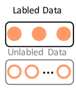
(a) SSL

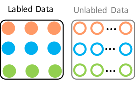
(b) SSDG

Figure 1: Comparison between the typical semi-supervised learning (SSL) and the semi-supervised domain generalization (SSDG). Note that different colors denote different domains. In the SSDG setting, there are multiple training domains with different data distributions when compared with SSL.

Several domain generalization methods have been developed to handle this issue [8, 9, 10, 11, 12, 13]. However, these methods need to label all data from source domains, which is expensive and time-consuming in real-world applications. In general, a few label for a dataset is readily to obtain, thus the semi-supervised domain generalization (SSDG) task is recently proposed [14], where there are a few labeled data in each source domain while most of samples do not have the label information. To tackle this task, StyleMatch [14] is proposed via extending the FixMatch [15] with a couple of new ingredients, which resorts to enhancing the diversity from the image level and the classifier level. However, this method does not handle the data-distribution discrepancy of different source domains, resulting in a negative on the accuracy of pseudo-labels during training.

Similarly, in the conventional semi-supervised learning (SSL), most of existing methods assume that all training samples are sampled from the same data distribution [16, 17, 18, 19, 20, 21, 22]. Differently, in the semi-supervised domain generation task, the training samples from different distributions, as illustrated in Fig. 1. Therefore, if directly using these methods to deal with the SSDG task, we cannot obtain the accurate pseudo-labels during the training course because the domain shift in the training set is not beneficial to producing the accurate pseudo-label.

In this paper, we mainly resort to obtaining accurate pseudo-labels so as to enhance the model’s discrimination and generalization in the unseen domain. We first analyze the generalization error on a domain using the theory of the multi-domain learning [23]. Based on the upper bound of the generalization error, we can obtain a conclusion that: 1) alleviating the interference of different domains and 2) using all samples to train the model can effectively reduce the upper bound of generalization error on each domain, which means that the accurate pseudo-labels can be generated.

Inspired by the theory of the multi-domain learning, we extend the FixMatch [15]  to a multi-task learning method, named MultiMatch, for semi-supervised domain generalization. Specifically, we build the independent local task for each domain to mitigate the interference from different domains during generating pseudo-labels. In addition, we also construct a jointly global task for predicting unseen target domain. Particularly, each independent local task is utilized to give the pseudo-label, while the jointly global task is trained using the pseudo-label. Furthermore, benefiting from the multi-task framework, we can fuse the predictions from the global and local tasks to further improve the accuracy of pseudo-labels and the generalization capability of the model in the training and test stages, respectively. We conduct a series of experiments on several DG benchmark datasets. Experimental results demonstrate the effectiveness of the proposed method, and the proposed method can produce a performance improvement when compared with the semi-supervised learning methods and the semi-supervised DG method. Moreover, we also verify the efficacy of each module in our method. In conclusion, our main contributions can be summarized as:

• We analyze the semi-supervised domain generalization task based on the generalization error of multi-domain learning, which inspires us to design a method to obtain the high-quality pseudo-label during training.

• We propose a simple yet effective multi-task learning (i.e., MultiMatch) for semi-supervised domain generalization, which can effectively reduce the interference from different domains during pseudo-labeling. Also, most of the modules in the model are shared for all domains, which can be sufficiently trained by all samples.

• To further promote the accuracy of pseudo-labels and the capability of the model, we propose to merge the outputs of the local task and the global task together to yield a robust prediction in the training and test stages.

• We evaluate our approach on multiple standard benchmark datasets, and the results show that our approach outperforms the state-of-the-art accuracy. Moreover, the ablation study and further analysis are provided to validate the efficacy of our method.

The rest of this paper is organized as follows. We review some related work in Section II. The proposed method is introduced in Section III. Experimental results and analysis are presented in Section IV, and Section V is conclusion.

II Related work

In this section, we investigate the related work to our work, including the semi-supervised learning methods and the domain generalization methods. The detailed investigation is presented in the following part.

II-A Semi-supervised Learning

The semi-supervise learning has achieved the remarkable performance in the recent years [16, 17, 18, 24, 25, 15, 26, 27, 19, 20, 21, 22, 28]. For example, Grandvalet et al.  [16] propose to minimize entropy regularization, which enables to incorporate unlabeled data in the standard supervised learning. Laine et al.  [17] develop Temporal Ensembling, which maintains an exponential moving average of label predictions on each training example, and penalizes predictions that are inconsistent with this target. However, because the targets change only once per epoch, Temporal Ensembling becomes unwieldy when learning large datasets. To overcome this issue, Tarvainen et al. [18] design Mean Teacher that averages model weights instead of label predictions. In FixMatch [15], the method first generates pseudo-labels using the model’s predictions on weakly-augmented unlabeled images, and is then trained to predict the pseudo-label when fed a strongly-augmented version of the same image. Furthermore, Zhang et al. [22] introduce a curriculum learning approach to leverage unlabeled data according to the model’s learning status. The core of the method is to flexibly adjust thresholds for different classes at each time step to let pass informative unlabeled data and their pseudo-labels.

However, the success of the typical SSL largely depends on the assumption that the labeled and unlabeled data share an identical class distribution, which is hard to meet in the real-world application. The distribution mismatch between the labeled and unlabeled sets can cause severe bias in the pseudo-labels of SSL, resulting in significant performance degradation. To bridge this gap, Zhao et al. [29] put forward a new SSL learning framework, named Distribution Consistency SSL, which rectifies the pseudo-labels from a distribution perspective. Differently, Oh et al. [30] propose a general pseudo-labeling framework that class-adaptively blends the semantic pseudo-label from a similarity-based classifier to the linear one from the linear classifier.

Different from these existing the semi-supervised learning settings, we aim to address the semi-supervised task with multiple domains in the training procedure, which results in the interference of different domains during pseudo-labeling because of the impact of the domain shift.

II-B Domain Generalization

Recently, some methods are also developed to address the domain generalization problem in some computer vision tasks [8, 9, 10, 31, 32, 33, 34, 13, 35, 36], such as classification and semantic segmentation. Inspired by domain adaptation methods, some works based on domain alignment [34, 37, 7, 38, 39, 40, 41] aim at mapping all samples from different domains into the same subspace to alleviate the difference of data distribution across different domains. For example, Muandet et al.  [7] introduce a kernel based optimization algorithm to learn the domain-invariant feature representation and enhance the discrimination capability of the feature representation. However, this method cannot grantee the consistency of conditional distribution, hence Zhao et al.  [37] develop an entropy regularization term to measure the dependency between the learned feature and the class labels, which can effectively ensure the conditional invariance of learned feature, so that the classifier can also correctly classify the feature from different domains.

Besides, Gong et al.  [40] exploit CycleGAN [42] to yield new styles of images that cannot be seen in the training set, which smoothly bridge the gap between source and target domains to boost the generalization of the model. Rahman et al.  [41] also employ GAN to generate synthetic data and then mitigate domain discrepancy to achieve domain generalization. Differently, Li et al.  [39] adopt an adversarial auto-encoder learning framework to learn a generalized latent feature representation in the hidden layer, and use Maximum Mean Discrepancy to align source domains, then they match the aligned distribution to an arbitrary prior distribution via adversarial feature learning. In this way, it can better generalize the feature of the hidden layer to other unknown domains. Rahman et al.  [38] incorporate the correlation alignment module along with adversarial learning to help achieve a more domain agnostic model because of the improved ability to more effectively reduce domain discrepancy. In addition to performing adversarial learning at the domain level to achieve domain alignment, Li et al.  [34] also conduct domain adversarial tasks at the class level to align samples of each category that from different domains.

Ideally, visual learning methods should be generalizable, for dealing with any unseen domain shift when deployed in a new target scenario, and it should be data-efficient for reducing development costs by using as little labels as possible. However, the conventional DG methods, which are unable to handle unlabeled data, perform poorly with limited labels in the SSDG task. To handle this task, Zhou et al. [14] propose StyleMatch, a simple approach that extends FixMatch with a couple of new ingredients tailored for SSDG: 1) stochastic modeling for reducing overfitting in scarce labels, and 2) multi-view consistency learning for enhancing the generalization capability of the model. However, StyleMatch cannot effectively address the interference of different domains during pseudo-labeling. In this paper, we deal with the SSDG task from the multi-task learning perspective.

III The proposed method

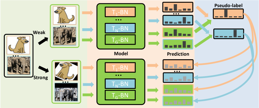
Figure 2: An illustration of the proposed MultiMatch for the semi-supervised domain generalization setting. In the method, training each domain is consider as the local task, and training all domains together is viewed as the global task. In the training course, we propose to employ the prediction fusion scheme to generate the final pseudo-label, which can be used to train the unlabeled samples.

In this paper, our goal is to address the semi-supervised domain generalization (SSDG) task. In this task, a few labeled samples on each domain are available, while most of samples lack the label information, thus a key task is how to generate the accurate pseudo-label. Different from the conventional semi-supervised methods, the SSDG task contains multiple source domains with different distributions. We first analyze the generalization error of multi-domain learning, which shows the upper bound of the generalization error is related to the discrepancy of different domains and the number of training samples. Particularly, reducing the upper bound is equal to improving the accuracy of the pseudo-label. Based on the analysis, we develop a multi-task learning method (i.e., MultiMatch) to deal with the SSDG task, as illustrated in Fig. 2. Besides, to further leverage the advantage of the multi-task learning framework, we fuse the predictions from different tasks to yield the better pseudo-label and more generalizable model in the training and test procedure. We will introduce our method in the following part.

III-A Theoretical Insight

In the semi-supervised DG task, each domain contains the labeled data and unlabeled data. To be specific, given $N$ domains in the training stage, we use $\mathcal{D}_{i}=\{\mathcal{D}_{i}^{l},\mathcal{D}_{i}^{u}\}$ to denote the $i$-th domain, where $\mathcal{D}_{i}^{l}$ and $\mathcal{D}_{i}^{u}$ represent the labeled and unlabeled samples in the $i$-th domain, respectively. Since there is no label information for $\mathcal{D}_{i}^{u}$, we aim to generate the high-quality pseudo-label in the training stage. Particularly, the SSDG task in the training stage can also be considered as multi-domain learning, and these unlabeled data can be viewed as the test data during pseudo-labeling. In the next part, we will introduce a theory of multi-domain learning to explore the semi-supervised DG task from the theoretical perspective.

Here, we consider hypotheses $h\in\mathcal{H}$ (i.e., prediction function), and give a vector $\alpha=(\alpha_{1},\ldots,\alpha_{N})$ of domain weights with $\sum_{j=1}^{N}\alpha_{j}=1$. In addition, we assume that the learner receives a total of $m$ labeled training samples, with $m_{j}=\beta_{j}m$ from the $j$-th domain $\mathcal{D}_{j}$. We define the empirical $\alpha$-weighted error of function $h$ as

$$\hat{\epsilon}_{\alpha}(h)=\sum_{j=1}^{N}\alpha_{j}\hat{\epsilon}_{j}(h)=\sum_{j=1}^{N}\frac{\alpha_{j}}{m_{j}}\sum_{x\in S_{j}}|h(x)-f_{j}(x)|,$$ (1)

where $f_{j}(x)$ is a labeling function for the $j$-th domain (i.e., the mapping from a sample to its ground truth).

Theorem 1 [23] Let $\mathcal{H}$ be a hypothesis space of VC dimension [43] $d$. For each domain $j\in\{1,...,N\}$, let $S_{j}$ be a labeled sample of size $\beta_{j}m$ generated by drawing $\beta_{j}m$ points from $\mathcal{D}_{j}$ and labeling them according to $f_{j}(\cdot)$. If $\hat{h}\in\mathcal{H}$ is the empirical minimizer of $\hat{\epsilon}_{\alpha}(h)$ for a fixed weight vector $\alpha$ on these samples and $h_{T}^{*}=\min_{h\in\mathcal{H}}\epsilon_{T}(h)$ is the target error minimizer, then the upper bound of the generalization error on the target domain $\mathcal{D}_{T}$, for any $\delta\in(0,1)$, with probability at least $1-\delta$, can be written as

$$\epsilon_{T}(\hat{h})\leqslant\epsilon_{T}(h_{T}^{*})+2\sqrt{(\sum_{j=1}^{N}\frac{\alpha_{j}^{2}}{\beta_{j}})\frac{d\log(2m)+\log(\delta)}{2m}}$$ (2)

$$+\sum_{j=1}^{N}\alpha_{j}(2\lambda_{j}+d_{\mathcal{H}\Delta\mathcal{H}}(\mathcal{D}_{j},\mathcal{D}_{T})),$$

where

$$\lambda_{j}=\min_{h\in\mathcal{H}}\{\epsilon_{T}(h)+\epsilon_{j}(h)\}.$$ (3)

The detailed demonstration process can be found in  [23].

In Eq. 2, the third term indicates the distribution discrepancy between $\mathcal{D}_{j}$ and $\mathcal{D}_{T}$. It is worth noting that, in the semi-supervised DG setting, all $\{\alpha_{i}\}_{i=1}^{N}$ and $\{\beta_{i}\}_{i=1}^{N}$ are $\frac{1}{N}$. Therefore, the Eq. 2 can be rewritten as

$$\epsilon_{T}(\hat{h})\leqslant\epsilon_{T}(h_{T}^{*})+\sum_{j=1}^{N}\frac{2\lambda_{j}}{N}+2\sqrt{\frac{d\log(2m)+\log(\delta)}{2m}}$$ (4)

$$+\sum_{j=1}^{N}\frac{1}{N}d_{\mathcal{H}\Delta\mathcal{H}}(\mathcal{D}_{j},\mathcal{D}_{T}).$$

According to Eq. 4, the upper bound of the generalization error on the target domain is mainly decided by four terms, where the first two terms can be considered as the constant. There are two observations in the third term and the fourth term. 1) In the third term, when $m$ is a larger value, the total value is smaller, which indicates that we should use the available samples to train the model. In other words, most modules in the designed model should be shared for all domains or tasks. 2) The last term is the distribution discrepancy between the source-target domain  and the other domains. If we can alleviate the discrepancy, the generalization error on the source-target domain can also be reduced.

Particularly, since the semi-supervised DG task consists of multiple domains, it can be also viewed as the multi-domain learning paradigm in the training stage. Besides, the unlabeled training data can be also considered as the test data during pseudo-labeling. Therefore, it means that, if we can effectively reduce the upper bound of the generalization error in Eq. 4, it will result in generating a high-quality pseudo-label for each domain in the training stage.

III-B Multi-task Learning Framework

FixMatch is a significant simplification of existing SSL methods [15]. It first generates pseudo-labels using the model’s predictions on weakly-augmented unlabeled images. For a given image, the pseudo-label is only retained if the model produces a high-confidence prediction. The model is then trained to predict the pseudo-label when fed a strongly-augmented version of the same image. Despite its simplicity, FixMatch achieves state-of-the-art performance across a variety of standard semi-supervised learning benchmarks. In the SSDG task, FixMatch also achieves better performance than other conventional semi-supervised methods [22, 21], which is verified in our experiment. In this paper, we aim to extend FixMatch to a multi-task framework.

Based on the upper bound of the generalization error in Eq. 4, the proposed method needs to satisfy two requirements: 1) most of modules in the model are shared for all domains, which can be sufficiently trained by all samples and 2) the model can reduce the interference of domain gap between different domains. Therefore, we propose a multi-task learning framework, named MultiMatch, to address the SSDG task.

In this part, we will describe our multi-task learning framework. Since there are multiple different domains in the SSDG task, we consider training each domain as an independent task (i.e., the local task for each domain), which can reduce the negative impact of different domains each other during pseudo-labeling. Besides, considering the SSDG task also needs to exploit in the unseen domain, we add a global task where we employ pseudo-labels from the local task to train the model. We assume that there are $N$ source domains in the training stage, thus we will build $N+1$ tasks in our framework. To be specific, we will employ the independent batch normalization (BN) [44] and classifier for each task in our method, and other modules are shared for all tasks. The batch normalization (BN) can be formulated by

$${\rm BN}(f_{d})=\gamma\frac{f_{d}-M_{\mu}(\phi)}{M_{\sigma}(\phi)}+\beta,~{}~{}d\in\phi,$$ (5)

where $\phi$ is the domain set, and $M_{\mu}(\phi)$ and $M_{\sigma}(\phi)$ represent the statistics for the $\phi$. When $\phi$ merely includes a domain, the sample will be normalized by the statistics from the own domain. Differently, when $\phi$ includes all domains, each sample will be normalized by the shared statistics from all domains. Since there exists a domain gap across different domains, the shared statistics will bring the noise error, as shown in the last term of Eq. 4, resulting in more generalization error.

Remark. In our multi-task learning framework, using the independent BN can effectively mitigate the interference of different domains, as shown in Eq. 4. In addition, in our method, most of modules are shared for all domains, which can sufficiently exploit all samples to reduce the third item in Eq. 4. Hence, our multi-task learning framework can obtain a small generalization error on each domain so as to generate an accurate pseudo-label for each domain in the training stage. Last but not least, the multi-task framework with multiple classifiers can produce the ensemble prediction for pseudo-label and test evaluation in the training and test procedure. We will give the prediction fusion scheme in the next part.

III-C Prediction Fusion

For an image $x_{i}$ from the $i$-th domain, we can generate its output $Y_{i}=[y_{1};\ldots;y_{N+1}]\in\mathbb{R}^{(N+1)\times C}$, where $C$ is the number of the classes. In the training stage, due to the interference of different domains each other, we employ the output of the $i$-th task as the main prediction. To further guarantee the reliability of pseudo-labels in the training course, we combine it with the output of the global task to generate the final pseudo-labels. For an image $x_{i}$ from the $i$-th domain, the pseudo-label is produced by

$${\rm Class}={\rm MaxClass}([y_{i};y_{N+1}]),$$ (6)

where ${\rm MaxClass}(\cdot)$ returns the column of the max value in a matrix. In the test stage, we use the output of the global task as the main perdition because the test domain is unseen (i.e., we do not know which training domain is similar to the test domain). Besides, for a test image, we also fuse the output of the most similar task to yield the final prediction result as

$$y_{max}={\rm MaxPath}([y_{1};\ldots;y_{N}]);$$ (7)

$${\rm Class}={\rm MaxClass}(\frac{y_{max}+y_{N+1}}{2}),$$ (8)

where ${\rm MaxPath}(\cdot)$ returns the prediction of the most similar task (i.e., the column has the maximum value in a matrix) for a test image in the test procedure.

III-D Training Process

In our method, we merely use the cross-entropy loss to train our model as in FixMatch [15]. In the training course, we randomly select the same number of labeled and unlabeled images from each domain to form a batch. It is worth noting that, each image passes the domain-specific BN and classifier, and all images are required to pass the global task. Simultaneously, we fuse the predictions of the domain-specific task and the global task together to generate the accurate pseudo-labels. The overall training process is shown in Algorithm 1.

Algorithm 1 The training procedure of the proposed MultiMatch

1:  Input: All training domains $\{\mathcal{D}_{i}^{l},\mathcal{D}_{i}^{u}\}_{i=1}^{N}$.

2:  Output: The trained parameters of the model $\theta$.

3:  Initialization: Initialize the parameters $\theta$.

4:  for iter $=<$ MaxIter do

5:     Generating a batch of images $\{\mathcal{B}^{l},\mathcal{B}^{u}\}.$

6:     Using the labeled samples $\mathcal{B}^{l}$ to train the model, each image passes the domain-specific BN and classifier, and all images pass the global BN and classifier.

7:     Conducting weak and strong augmentations for $\mathcal{B}^{u}$ to generate $\mathcal{B}_{w}^{u}$ and $\mathcal{B}_{s}^{u}$.

8:     Based on $\mathcal{B}_{w}^{u}$ to yield the pseudo-label $Y_{u}$ by Eq. 6.

9:     Using $\mathcal{B}_{s}^{u}$ and $Y_{u}$ to train the model, and the forward path of all images is consistent with $\mathcal{B}^{l}$.

10:  end for

IV Experiments

In this section, we firstly introduce the experimental datasets and settings in Section IV-A. Then, we compare the proposed MultiMatch with the state-of-the-art SSL methods and the SSDG method in Section IV-B, respectively. To validate the effectiveness of various components in our MultiMatch, we conduct ablation studies in Section IV-C. Lastly, we further analyze the property of the proposed method in Section IV-D.

IV-A Datasets and Experimental Settings

IV-A1 Datasets

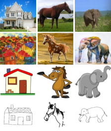
(a) PACS

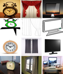
(b) Office-Home

Figure 3: Examples on PACS and Office-Home, respectively. It is worth noting that different rows denote different domains.

In this paper, we conduct the experiments to validate the effectiveness of our method on three benchmark DG datasets as follows:

• PACS [45] consists of four different domains: Photo, Art, Cartoon and Sketch. It contains 9,991 images with 7 object categories in total, including Photo (1,670 images), Art (2,048 images), Cartoon (2,344 images), and Sketch (3,929 images).

• Office-Home [46] contains 15,588 images of 65 categories of office and home objects. It has four different domains namely Art (2,427 images), Clipart (4,365 images), Product (4,439 images) and Real World (4,357 images), which is originally introduced for UDA but is also applicable in the DG setting.

• miniDomainNet [47] takes a subset of DomainNet [48] and utilizes a smaller image size (96 $\times$ 96). miniDomainNet includes four domains and 126 classes. As a result, miniDomainNet contains 18,703 images of Clipart, 31,202 images of Painting, 65,609 images of Real and 24,492 images of Sketch.

We show some examples from PACS and Office-home in Fig. 3. As seen, there is an obvious difference among different domains. Besides, we also visualize the features of four categories on PACS by t-SNE [49], as illustrated in Fig. 4. In this figure, different colors are different domains. We observe that different domains appear in different spaces, which validates that there exists the domain shift in the training set.

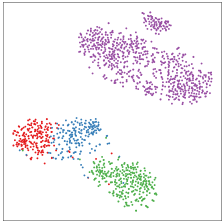
(a) Horse

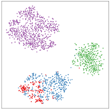
(b) Dog

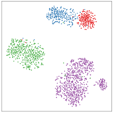
(c) Elephant

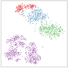
(d) Giraffe

Figure 4: Visualization of the feature representation on four classes of PACS by t-SNE [49]. The features are extracted by ResNet18 pre-trained on ImageNet [50]. Note that different colors indicate different domains.

IV-A2 Implementation Details

Following the common practice [51], ResNet18 [1] pre-trained on ImageNet [50] is employed as the CNN backbone (for all models compared in this paper). We randomly sample 64 images from each source domain to construct a minibatch for labeled and unlabeled data, respectively. The initial learning rate is set as $0.003$ for the pre-trained backbone. In the experiment, to enrich the diversity of the augmentation, we integrate the AdaIN augmentation [52] into the strong augmentation scheme. Particularly, the augmentation scheme is utilized in all experiments, including the baseline (i.e., FixMatch), thus it is a fair comparison in the experiment.

IV-B Comparison with State-of-the-art Methods

We conduct the experiment to compare our method with some semi-supervised learning methods (i.e., MeanTeacher [18], EntMin [16], DebiasPL [21], FlexMatch [22], FixMatch [15]) and the semi-supervised DG method (i.e., StyleMatch [14]). In this experiment, we run these methods under two different settings (i.e., 10 labels per class and 5 labels per class) on three benchmark datasets. The experimental results are reported in Table I. As seen in this table, among these typical semi-supervised methods, FixMatch can achieve the best performance. Compared with FixMatch, our method can further improve the performance. For example, on PACS our method outperforms FixMatch by $+3.74\%$ ($81.57$ vs. $77.83$) and $+5.09\%$ ($80.04$ vs. $74.95$) under the “10 labels per class” case and the “5 labels per class” case, respectively. Besides, on the large-scale dataset (i.e., miniDomainNet), our method can also achieve an obvious improvement, which is attributed to the fact that our method reduces the interference of different domains while guaranteeing that all training samples are utilized to train the model.

In addition, StyleMatch is developed to address the semi-supervised domain generalization task. Compared with it, our method has better experimental results on all settings and datasets, except for the “5 labels per class” case on PACS. For example, on miniDomainNet, our method increases StyleMatch by $+3.66\%$ ($58.79$ vs. $55.13$) and $+3.57\%$ ($54.61$ vs. $51.04$) under the “10 labels per class” case and the “5 labels per class” case, respectively. This confirms the effectiveness of our method when compared with the SOTA method, which thanks to the advantage of the multi-task learning framework in the semi-supervised domain generalization task. The effectiveness of each module in our proposed MultiMatch will be verified in the next ablation study.

TABLE I: Comparison between our method and different semi-supervised (DG) methods under different numbers of labeled samples on PACA, Office-Home and miniDomainNet. Note that “P”, “A”, “C” and “S” denote different domains on PACS. “Avg” is the average result of all domains. The bold is the best result.

	PACS					Office-Home					miniDomainNet
Method	P	A	C	S	Avg	A	C	P	R	Avg	C	P	R	S	Avg
	10 labels per class
MeanTeacher [18]	85.95	62.41	57.94	47.66	63.49	49.92	43.42	64.61	68.79	56.69	46.75	49.48	60.98	37.05	48.56
EntMin [16]	89.39	72.77	70.55	54.38	71.77	51.92	44.92	66.85	70.52	58.55	46.96	49.59	61.10	37.26	48.73
FlexMatch [22]	66.04	48.44	60.79	53.23	57.13	25.63	28.25	37.98	36.15	32.00	38.97	32.44	39.34	11.82	30.64
DebiasPL [21]	93.23	74.60	67.23	63.49	74.64	44.71	38.62	64.42	68.39	54.04	54.18	54.27	57.53	47.93	53.48
FixMatch [15]	87.40	76.85	69.40	77.68	77.83	49.90	50.98	63.79	66.75	57.86	51.22	54.99	59.53	52.45	54.55
StyleMatch [14]	90.04	79.43	73.75	78.40	80.41	52.82	51.60	65.31	68.61	59.59	52.76	56.15	58.72	52.89	55.13
MultiMatch (ours)	93.25	83.30	73.00	76.74	81.57	56.32	52.76	68.94	72.28	62.57	56.13	59.15	63.68	56.18	58.79
	5 labels per class
MeanTeacher [18]	73.54	56.00	52.64	36.97	54.79	44.65	39.15	59.18	62.98	51.49	39.01	42.92	54.40	31.13	41.87
EntMin [16]	79.99	67.01	65.67	47.96	65.16	48.11	41.72	62.41	63.97	54.05	39.39	43.35	54.80	31.72	42.32
FlexMatch [22]	61.80	23.83	37.28	48.09	42.75	19.04	26.16	30.81	23.00	24.75	13.80	20.52	17.88	20.40	18.15
DebiasPL [21]	89.52	65.52	54.09	29.22	59.59	41.41	33.45	58.77	60.59	48.56	50.87	52.11	51.86	44.61	49.86
FixMatch [15]	86.15	74.34	69.08	73.11	75.67	46.60	48.74	59.65	63.21	54.55	47.23	52.88	55.99	52.88	52.24
StyleMatch [14]	89.25	78.54	74.44	79.06	80.32	51.53	50.00	60.88	64.47	56.72	46.30	52.63	54.65	50.59	51.04
MultiMatch (ours)	90.66	82.43	72.43	74.64	80.04	53.71	50.21	63.99	67.81	58.93	50.99	56.03	58.53	52.88	54.61

IV-C Ablation Studies

In the experiment, we first validate the effectiveness of the multi-task learning framework, and then analyze the efficacy of the fusion prediction scheme in the training stage and the test stage, respectively. The experimental results are shown in Table II, where “MTL+TRAIN-local+TEST-global” denotes that the pseudo-labels are generated by the domain-specific path (i.e., local task), and the final prediction during test is based on the global task. In other words, “MTL+TRAIN-local+TEST-global” means that we do not utilize the fusion prediction scheme in both the training and test stages. “MTL+TRAIN-global-local+TEST-global-local” indicates that we employ the fusion prediction scheme in both the training and test stages.

As seen in Table II, “MTL+TRAIN-local+TEST-global” outperforms “Baseline” on both PACS and Office-Home, which confirms the effectiveness of the multi-task learning framework in the semi-supervised domain generalization task. For example, the multi-task learning framework can bring an obvious improvement by $+3.37\%$ ($61.23$ vs. $57.86$) on Office-Home. In addition, the fusion prediction scheme is also effective in both the training and test stages. As seen in Table II, “MTL+TRAIN-global-local+TEST-global” outperforms “MTL+TRAIN-local+TEST-global”, and “MTL+TRAIN-global-local+TEST-global-local” outperforms “MTL+TRAIN-local+TEST-global-local”, which indicates the effectiveness of the fusion prediction scheme in the training stage. Meanwhile, “MTL+TRAIN-local+TEST-global-local ” outperforms “MTL+TRAIN-local+TEST-global”, and “MTL+TRAIN-global-local+TEST-global-local” outperforms “MTL+TRAIN-global-local+TEST-global”, which confirms the effectiveness of the fusion prediction scheme in the test stage. In our method, we use the fusion manner in Section III-C. We will also investigate some other fusion manners in further analysis.

TABLE II: Ablation studies on different components of our method on PACS and Office-Home under the case with 10 labels per class. To better show the best result, we only use bold on the best average result.

Method	PACS					Office-Home
	P	A	C	S	Avg	A	C	P	R	Avg
Baseline (FixMatch)	87.40	76.85	69.40	77.68	77.83	49.90	50.98	63.79	66.75	57.86
MTL+TRAIN-local+TEST-global	92.63	77.28	68.52	74.15	78.15	55.04	51.24	67.41	71.21	61.23
MTL+TRAIN-local+TEST-global-local	93.37	83.43	70.15	75.71	80.67	56.13	51.70	68.20	71.71	61.94
MTL+TRAIN-global-local+TEST-global	92.22	77.08	68.72	75.05	78.27	55.31	52.36	68.17	71.58	61.86
MTL+TRAIN-global-local+TEST-global-local	93.25	83.30	73.00	76.74	81.57	56.32	52.76	68.94	72.28	62.57

IV-D Further Analysis

Evaluation on different fusion manners. In this part, we evaluate different fusion manners in our framework on PACS. Experimental results are listed in Table III. Each fusion manner is described in the following formulas. “TEST-avg-all” is the mean of the outputs from all tasks in the testing stage. “TEST-max” denotes the maximum output among all tasks in the testing stage. “TRAIN-avg” means using the mean of outputs from the own task and the global task during pseudo-labeling. As observed in Table III, “TRAIN-max+TEST-avg” (i.e., Eq. 6 and Eq. 8) can obtain the slight improvement when compared with other fusion scheme. Besides, compared with the “MTL+TRAIN-local+TEST-global” (i.e., without using the fusion scheme in our method), all schemes in Table III outperform it, which indicates that the prediction’s ensemble is significant for our method during training and testing.

TEST-avg-all:

$${\rm Class}={\rm MaxClass}(\frac{y_{1}+\ldots+y_{N+1}}{N+1}).$$

TEST-max:

$${\rm Class}={\rm MaxClass}([y_{max};y_{N+1}]),$$

where $y_{max}$ is defined in Eq. 7.

TRAIN-avg:

$${\rm Class}={\rm MaxClass}(\frac{y_{i}+y_{N+1}}{2}),$$

where $y_{i}$ is the perdition of an image from the $i$-th domain.

TABLE III: Experimental results of different label-fusion schemes on PACS under the case with 10 labels per class.

Fusion scheme	P	A	C	S	Avg
TRAIN-max+TEST-avg (ours)	93.25	83.30	73.00	76.74	81.57
TRAIN-max+TEST-avg-all	93.36	83.32	72.34	76.76	81.44
TRAIN-max+TEST-max	92.93	83.24	72.76	76.76	81.42
TRAIN-avg+TEST-avg	93.45	83.56	71.26	76.89	81.29
TRAIN-avg+TEST-avg-all	93.46	83.49	71.35	76.82	81.28
TRAIN-avg+TEST-max	93.29	83.59	71.08	76.96	81.23

The accuracy of pseudo-labels. In this experiment, we evaluate the accuracy of pseudo-labels of different methods on Precision, Recall and macro-f1. It is worth noting that macro-f1 fuses Recall and Precision together. Table IV shows the experimental results, where “MTL+TRAIN-local” represents the accuracy of the pseudo-labels from the domain-specific classifier in our method, and “MTL+TRAIN-global-local” is the accuracy of the pseudo-labels generated by fusing the domain-specific classifier and the global classifier in our method. As observed in Table IV, “MTL+TRAIN-local” can improve the macro-f1 of FixMatch by $+1.37$ ($90.63$ vs. $89.26$) and $+1.27$ ($70.41$ vs. $69.14$) on PACS and Office-Home, respectively. This validates that using the independent task for each domain can indeed alleviate the interference of different domains so as to improve the pseudo-labels of unlabeled data. Besides, “MTL+TRAIN-global-local” outperforms all other methods, e.g., “MTL+TRAIN-global-local” increases the macro-f1 of StyleMatch by $+1.35$ ($92.70$ vs. $91.35$) and $+2.39$ ($73.07$ vs. $70.68$) on on PACS and Office-Home, respectively. Therefore, this confirms our method can achieve better accuracy of pseudo-labels to enhance the generalization capability of the model. Furthermore, we also display the accuracy of pseudo-labels of different methods at different epochs on PACS and Office-Home in Fig. 5, respectively. As seen, our method can give more accurate pseudo-labels at each epoch when compared with FixMatch and StyleMatch.

TABLE IV: The accuracy of pseudo-labels of different methods on PACS and Office-Home under the case with 10 labels per class.

Dataset	Method	Precision	Recall	macro-f1
PACS	FixMatch	88.83	89.52	89.26
	StyleMatch	90.84	91.52	91.35
	MTL+TRAIN-local	90.17	90.86	90.63
	MTL+TRAIN-global-local	92.23	92.82	92.70
Office-Home	FixMatch	71.05	69.97	69.14
	StyleMatch	72.67	71.41	70.68
	MTL+TRAIN-local	72.22	71.25	70.41
	MTL+TRAIN-global-local	74.86	73.76	73.07

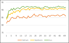
(a) PACS

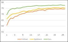
(b) Office-Home

Figure 5: The accuracy of pseudo-labels of different methods at different epochs on PACS and Office-Home, respectively.

Test on different numbers of the labeled data. We also conduct the comparison between our proposed MultiMatch and StyleMatch under different numbers of the labeled data on PACS, as shown in Fig. 6. According to this figure, except for the “5 labels per class” case, our MultiMatch obviously outperforms StyleMatch in all other cases. For example, when we use 160 labels per class, our MultiMatch improves the performance by $+1.1\%$ ($83.43$ vs. $82.33$) when compared with StyleMatch. Besides, given the label information for all training samples, our method can also obtain better results than StyleMatch.

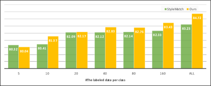
Figure 6: Comparison between our MultiMatch and StyleMatch under different numbers of the labeled data on PACS. “ALL” denotes that all training samples have label information during training.

Evaluation on the independent BN and the independent classifier. In this part, we validate the effectiveness of the independent BN and the independent classifier in our method. Experimental results are listed in Table V, where “w/ SBN” and “w/ SC” indicate using the shared BN and the shared classifier in our method, respectively. As observed in Table V, using the independent BN and the independent classifier together can yield better performance than using the independent BN or the independent classifier. For example, our method improve the “w/ SBN” and “w/ SC” by $+1.44\%$ ($81.57$ vs. $80.13$) and $+2.47\%$ ($81.57$ vs. $79.10$) on PACS, respectively. Besides, compared with the original FixMatch in Table I under “10 labels per class”, both “w/ SBN” and “w/ SC” outperform them on PACS and Office-Home. All the above observations confirm the effectiveness of both the independent BN and the independent classifier in our method.

TABLE V: Evaluation on the independent BN and the independent classifier on PACS and Office-Home, respectively.

Module	PACS
	P	A	C	S	Avg
w/ SBN	91.62	82.09	73.10	73.70	80.13
w/ SC	91.07	78.10	71.12	76.12	79.10
Ours	93.25	83.30	73.00	76.74	81.57
Module	Office-Home
	A	C	P	R	Avg
w/ SBN	55.30	51.65	68.01	71.56	61.63
w/ SC	54.68	52.28	67.38	71.22	61.39
Ours	56.32	52.76	68.94	72.28	62.57

Effectiveness of the unlabeled data in SSDG. To validate the effectiveness of the unlabeled data in SSDG, we train the supervised DG methods using the labeled samples, including ResNet18, CrossGrad [53], DDAIG [54], RSC [51]. Experimental results are shown in Fig. 7. As observed in this figure, using the unlabeled data can obtain better performance than these conventional DG methods with the labeled data, which validates that the unlabeled samples are very meaningful in the SSDG task. Furthermore, our MultiMatch can effectively mine the information from these unlabeled data, which has been reported in Table I.

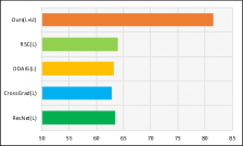
(a) PACS

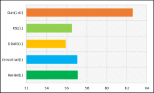
(b) Office-Home

Figure 7: Experimental results of the typical DG methods under the labeled samples in SSDG on PACS and Office-Home, respectively. Note that “L” denotes only using the labeled samples, and “L+U” is using the labeled and unlabeled samples together.

Test on the supervised case. In the experiment, we train our model in the supervised setting, and compare it with some supervised DG methods, as reported in Tables VI and VII. MLDG [55], MASF [56] and MetaReg [32] are meta-learning based methods. FACT [57], RSC [51] and FSDCL [58] are augmentation based methods. In addition, VDN [59] and SNR [60] aim at learning domain-invariant features, and DAEL [47] is a ensemble learning based method. Compared with these supervised methods, our MultiMatch is also competitive in the supervised case.

TABLE VI: Experimental results of different methods under the supervised setting on PACS. The bold and gray are the best result and the second-best result, respectively.

Method	P	A	C	S	Avg
MLDG [55]	94.30	79.50	77.30	71.50	80.65
MASF [56]	94.99	80.29	77.17	71.69	81.04
MetaReg [32]	95.50	83.70	77.20	70.30	81.68
SNR [60]	94.50	80.3	78.20	74.10	81.80
VDN [59]	94.00	82.60	78.50	82.70	84.45
FACT [57]	95.15	85.37	78.38	79.15	84.51
MultiMatch (ours)	95.79	84.44	75.83	82.82	84.72

TABLE VII: Experimental results of different methods under the supervised setting on Office-Home.

Method	A	C	P	R	Avg
RSC [51]	58.42	47.90	71.63	74.54	63.12
DAEL [47]	59.40	55.10	74.00	75.70	66.05
SNR [60]	61.20	53.70	74.20	75.10	66.10
FSDCL [58]	60.24	53.54	74.36	76.66	66.20
FACT [57]	60.34	54.85	74.48	76.55	66.56
MultiMatch (ours)	59.71	56.25	74.28	75.70	66.49

V Conclusion

In this paper, we aim to tackle the semi-supervised domain generalization (SSDG) task. Different from the typical semi-supervised task, the challenge of SSDG is that there exist multiple different domains with the latent distribution discrepancy. To address this issue, we first explore the theory of multi-domain learning to generate more accurate pseudo-labels for unlabeled samples. Then, we propose to utilize a multi-task learning framework to mitigate the impact of the domain discrepancy and sufficiently exploit all training samples, which can effectively enhance the model’s generalization. We conduct the experiment on multiple benchmark datasets, which verifies the effectiveness of the proposed method.

References

- [1] K. He, X. Zhang, S. Ren, and J. Sun, “Deep residual learning for image recognition,” in IEEE Conference on Computer Vision and Pattern Recognition (CVPR), 2016, pp. 770–778.
- [2] S. Ren, K. He, R. B. Girshick, and J. Sun, “Faster R-CNN: towards real-time object detection with region proposal networks,” IEEE Transactions on Pattern Analysis and Machine Intelligence (TPAMI), vol. 39, no. 6, pp. 1137–1149, 2017.
- [3] J. Devlin, M.-W. Chang, K. Lee, and K. Toutanova, “Bert: Pre-training of deep bidirectional transformers for language understanding,” arXiv preprint arXiv:1810.04805, 2018.
- [4] H. Luo, W. Jiang, Y. Gu, F. Liu, X. Liao, S. Lai, and J. Gu, “A strong baseline and batch normalization neck for deep person re-identification,” IEEE Transactions on Multimedia (TMM), vol. 22, no. 10, pp. 2597–2609, 2020.
- [5] J. Wang, C. Lan, C. Liu, Y. Ouyang, and T. Qin, “Generalizing to unseen domains: A survey on domain generalization,” in International Joint Conference on Artificial Intelligence (IJCAI), 2021, pp. 4627–4635.
- [6] K. Zhou, Z. Liu, Y. Qiao, T. Xiang, and C. C. Loy, “Domain generalization: A survey,” IEEE Transactions on Pattern Analysis and Machine Intelligence (TPAMI), 2022.
- [7] K. Muandet, D. Balduzzi, and B. Schölkopf, “Domain generalization via invariant feature representation,” in International Conference on Machine Learning (ICML), 2013, pp. 10–18.
- [8] H. Nam, H. Lee, J. Park, W. Yoon, and D. Yoo, “Reducing domain gap by reducing style bias,” in IEEE Conference on Computer Vision and Pattern Recognition (CVPR), 2021, pp. 8690–8699.
- [9] S. Seo, Y. Suh, D. Kim, G. Kim, J. Han, and B. Han, “Learning to optimize domain specific normalization for domain generalization,” in European Conference on Computer Vision (ECCV), 2020, pp. 68–83.
- [10] X. Yue, Y. Zhang, S. Zhao, A. L. Sangiovanni-Vincentelli, K. Keutzer, and B. Gong, “Domain randomization and pyramid consistency: Simulation-to-real generalization without accessing target domain data,” in International Conference on Computer Vision (ICCV), 2019, pp. 2100–2110.
- [11] Y. Wang, L. Qi, Y. Shi, and Y. Gao, “Feature-based style randomization for domain generalization,” IEEE Transactions on Circuits and Systems for Video Technology (TCSVT), vol. 32, no. 8, pp. 5495–5509, 2022.
- [12] L. Qi, L. Wang, Y. Shi, and X. Geng, “A novel mix-normalization method for generalizable multi-source person re-identification,” IEEE Transactions on Multimedia (TMM), 2022.
- [13] J. Zhang, L. Qi, Y. Shi, and Y. Gao, “Generalizable model-agnostic semantic segmentation via target-specific normalization,” Pattern Recognition (PR), vol. 122, p. 108292, 2022.
- [14] K. Zhou, C. C. Loy, and Z. Liu, “Semi-supervised domain generalization with stochastic stylematch,” arXiv preprint arXiv:2106.00592, 2021.
- [15] K. Sohn, D. Berthelot, N. Carlini, Z. Zhang, H. Zhang, C. Raffel, E. D. Cubuk, A. Kurakin, and C. Li, “Fixmatch: Simplifying semi-supervised learning with consistency and confidence,” in Advances in Neural Information Processing Systems (NeurIPS), 2020.
- [16] Y. Grandvalet and Y. Bengio, “Semi-supervised learning by entropy minimization,” in Advances in Neural Information Processing Systems (NeurIPS), 2004, pp. 529–536.
- [17] S. Laine and T. Aila, “Temporal ensembling for semi-supervised learning,” in International Conference on Learning Representations (ICLR), 2017.
- [18] A. Tarvainen and H. Valpola, “Mean teachers are better role models: Weight-averaged consistency targets improve semi-supervised deep learning results,” in Advances in Neural Information Processing Systems (NeurIPS), 2017, pp. 1195–1204.
- [19] I. Nassar, S. Herath, E. Abbasnejad, W. Buntine, and G. Haffari, “All labels are not created equal: Enhancing semi-supervision via label grouping and co-training,” in IEEE Conference on Computer Vision and Pattern Recognition (CVPR), 2021, pp. 7241–7250.
- [20] M. Zheng, S. You, L. Huang, F. Wang, C. Qian, and C. Xu, “Simmatch: Semi-supervised learning with similarity matching,” in IEEE Conference on Computer Vision and Pattern Recognition (CVPR), 2022, pp. 14 471–14 481.
- [21] X. Wang, Z. Wu, L. Lian, and S. X. Yu, “Debiased learning from naturally imbalanced pseudo-labels,” in IEEE Conference on Computer Vision and Pattern Recognition (CVPR), 2022, pp. 14 647–14 657.
- [22] B. Zhang, Y. Wang, W. Hou, H. Wu, J. Wang, M. Okumura, and T. Shinozaki, “Flexmatch: Boosting semi-supervised learning with curriculum pseudo labeling,” in Advances in Neural Information Processing Systems (NeurIPS), 2021, pp. 18 408–18 419.
- [23] S. Ben-David, J. Blitzer, K. Crammer, A. Kulesza, F. Pereira, and J. W. Vaughan, “A theory of learning from different domains,” Machine Learning (ML), vol. 79, no. 1, pp. 151–175, 2010.
- [24] D. Berthelot, N. Carlini, I. J. Goodfellow, N. Papernot, A. Oliver, and C. Raffel, “Mixmatch: A holistic approach to semi-supervised learning,” in Advances in Neural Information Processing Systems (NeurIPS), 2019, pp. 5050–5060.
- [25] D. Berthelot, N. Carlini, E. D. Cubuk, A. Kurakin, K. Sohn, H. Zhang, and C. Raffel, “Remixmatch: Semi-supervised learning with distribution matching and augmentation anchoring,” in International Conference on Learning Representations (ICLR), 2020.
- [26] J. Li, C. Xiong, and S. C. Hoi, “Comatch: Semi-supervised learning with contrastive graph regularization,” in International Conference on Computer Vision (ICCV), 2021, pp. 9475–9484.
- [27] C. Gong, D. Wang, and Q. Liu, “Alphamatch: Improving consistency for semi-supervised learning with alpha-divergence,” in IEEE Conference on Computer Vision and Pattern Recognition (CVPR), 2021, pp. 13 683–13 692.
- [28] F. Yang, K. Wu, S. Zhang, G. Jiang, Y. Liu, F. Zheng, W. Zhang, C. Wang, and L. Zeng, “Class-aware contrastive semi-supervised learning,” in Proceedings of the IEEE/CVF Conference on Computer Vision and Pattern Recognition (CVPR), June 2022, pp. 14 421–14 430.
- [29] Z. Zhao, L. Zhou, Y. Duan, L. Wang, L. Qi, and Y. Shi, “Dc-ssl: Addressing mismatched class distribution in semi-supervised learning,” in IEEE Conference on Computer Vision and Pattern Recognition (CVPR), 2022, pp. 9757–9765.
- [30] Y. Oh, D.-J. Kim, and I. S. Kweon, “Daso: Distribution-aware semantics-oriented pseudo-label for imbalanced semi-supervised learning,” in IEEE Conference on Computer Vision and Pattern Recognition (CVPR), 2022, pp. 9786–9796.
- [31] F. M. Carlucci, A. D’Innocente, S. Bucci, B. Caputo, and T. Tommasi, “Domain generalization by solving jigsaw puzzles,” in IEEE Conference on Computer Vision and Pattern Recognition (CVPR), 2019, pp. 2229–2238.
- [32] Y. Balaji, S. Sankaranarayanan, and R. Chellappa, “Metareg: Towards domain generalization using meta-regularization,” in Advances in Neural Information Processing Systems (NeurIPS), 2018, pp. 1006–1016.
- [33] D. Li, J. Zhang, Y. Yang, C. Liu, Y. Song, and T. M. Hospedales, “Episodic training for domain generalization,” in International Conference on Computer Vision (ICCV), 2019, pp. 1446–1455.
- [34] Y. Li, X. Tian, M. Gong, Y. Liu, T. Liu, K. Zhang, and D. Tao, “Deep domain generalization via conditional invariant adversarial networks,” in European Conference on Computer Vision (ECCV), 2018, pp. 647–663.
- [35] Y. Liu, Z. Xiong, Y. Li, X. Tian, and Z.-J. Zha, “Domain generalization via encoding and resampling in a unified latent space,” IEEE Transactions on Multimedia (TMM), 2021.
- [36] Z. Zhou, L. Qi, X. Yang, D. Ni, and Y. Shi, “Generalizable cross-modality medical image segmentation via style augmentation and dual normalization,” in Proceedings of the IEEE/CVF Conference on Computer Vision and Pattern Recognition (CVPR), June 2022, pp. 20 856–20 865.
- [37] S. Zhao, M. Gong, T. Liu, H. Fu, and D. Tao, “Domain generalization via entropy regularization,” in Advances in Neural Information Processing Systems (NeurIPS), 2020.
- [38] M. M. Rahman, C. Fookes, M. Baktashmotlagh, and S. Sridharan, “Correlation-aware adversarial domain adaptation and generalization,” Pattern Recognition (PR), vol. 100, p. 107124, 2020.
- [39] H. Li, S. J. Pan, S. Wang, and A. C. Kot, “Domain generalization with adversarial feature learning,” in IEEE Conference on Computer Vision and Pattern Recognition (CVPR), 2018, pp. 5400–5409.
- [40] R. Gong, W. Li, Y. Chen, and L. V. Gool, “DLOW: domain flow for adaptation and generalization,” in IEEE Conference on Computer Vision and Pattern Recognition (CVPR), 2019, pp. 2477–2486.
- [41] M. M. Rahman, C. Fookes, M. Baktashmotlagh, and S. Sridharan, “Multi-component image translation for deep domain generalization,” in IEEE Winter Conference on Applications of Computer Vision (WACV), 2019, pp. 579–588.
- [42] J. Zhu, T. Park, P. Isola, and A. A. Efros, “Unpaired image-to-image translation using cycle-consistent adversarial networks,” in International Conference on Computer Vision (ICCV), 2017, pp. 2242–2251.
- [43] T. Hastie, R. Tibshirani, J. H. Friedman, and J. H. Friedman, The elements of statistical learning: data mining, inference, and prediction, 2009, vol. 2.
- [44] W. Chang, T. You, S. Seo, S. Kwak, and B. Han, “Domain-specific batch normalization for unsupervised domain adaptation,” in IEEE Conference on Computer Vision and Pattern Recognition (CVPR), 2019, pp. 7354–7362.
- [45] D. Li, Y. Yang, Y.-Z. Song, and T. M. Hospedales, “Deeper, broader and artier domain generalization,” in International Conference on Computer Vision (ICCV), 2017, pp. 5543–5551.
- [46] H. Venkateswara, J. Eusebio, S. Chakraborty, and S. Panchanathan, “Deep hashing network for unsupervised domain adaptation,” in CVPR, 2017, pp. 5018–5027.
- [47] K. Zhou, Y. Yang, Y. Qiao, and T. Xiang, “Domain adaptive ensemble learning,” IEEE Transactions Image Process (TIP), vol. 30, pp. 8008–8018, 2021.
- [48] X. Peng, Q. Bai, X. Xia, Z. Huang, K. Saenko, and B. Wang, “Moment matching for multi-source domain adaptation,” in International Conference on Computer Vision (ICCV), 2019, pp. 1406–1415.
- [49] L. Van der Maaten and G. Hinton, “Visualizing data using t-sne,” Journal of machine learning research (JMLR), vol. 9, no. 11, pp. 2579–2605, 2008.
- [50] J. Deng, W. Dong, R. Socher, L. Li, K. Li, and F. Li, “Imagenet: A large-scale hierarchical image database,” in IEEE Conference on Computer Vision and Pattern Recognition (CVPR), 2009, pp. 248–255.
- [51] Z. Huang, H. Wang, E. P. Xing, and D. Huang, “Self-challenging improves cross-domain generalization,” in European Conference on Computer Vision (ECCV), 2020, pp. 124–140.
- [52] X. Huang and S. J. Belongie, “Arbitrary style transfer in real-time with adaptive instance normalization,” in International Conference on Computer Vision (ICCV), 2017, pp. 1510–1519.
- [53] S. Shankar, V. Piratla, S. Chakrabarti, S. Chaudhuri, P. Jyothi, and S. Sarawagi, “Generalizing across domains via cross-gradient training,” in International Conference on Learning Representations (ICLR), 2018.
- [54] K. Zhou, Y. Yang, T. M. Hospedales, and T. Xiang, “Deep domain-adversarial image generation for domain generalisation,” in AAAI Conference on Artificial Intelligence (AAAI), 2020, pp. 13 025–13 032.
- [55] D. Li, Y. Yang, Y. Song, and T. M. Hospedales, “Learning to generalize: Meta-learning for domain generalization,” in AAAI Conference on Artificial Intelligence (AAAI), 2018, pp. 3490–3497.
- [56] Q. Dou, D. C. de Castro, K. Kamnitsas, and B. Glocker, “Domain generalization via model-agnostic learning of semantic features,” in Advances in Neural Information Processing Systems (NeurIPS), 2019, pp. 6447–6458.
- [57] Q. Xu, R. Zhang, Y. Zhang, Y. Wang, and Q. Tian, “A fourier-based framework for domain generalization,” in IEEE Conference on Computer Vision and Pattern Recognition (CVPR), 2021, pp. 14 383–14 392.
- [58] S. Jeon, K. Hong, P. Lee, J. Lee, and H. Byun, “Feature stylization and domain-aware contrastive learning for domain generalization,” in ACM International Conference on Multimedia (MM), 2021, pp. 22–31.
- [59] Y. Wang, H. Li, L.-P. Chau, and A. C. Kot, “Variational disentanglement for domain generalization,” arXiv preprint arXiv:2109.05826, 2021.
- [60] X. Jin, C. Lan, W. Zeng, and Z. Chen, “Style normalization and restitution for domain generalization and adaptation,” IEEE Transactions on Multimedia (TMM), vol. 24, pp. 3636–3651, 2022.