Equation of state of a hot-and-dense quark gluon plasma:
lattice simulations at real $\mu_{B}$ vs. extrapolations

Abstract

The equation of state of the quark gluon plasma is a key ingredient of heavy ion phenomenology. In addition to the traditional Taylor method, several novel approximation schemes have been proposed with the aim of calculating it at finite baryon density. In order to gain a pragmatic understanding of the limits of these schemes, we compare them to direct results at $\mu_{B}>0$, using reweighting techniques free from an overlap problem. We use 2stout improved staggered fermions with 8 time-slices and cover the entire RHIC BES range in the baryochemical potential, up to $\mu_{B}/T=3$.

Introduction

The equation of state of strongly interacting matter under extreme conditions - high temperatures or baryon densities - plays a key role in many physical systems, such as the early Universe, heavy ion collisions and neutron stars. The most well established first-principles method to study the strongly coupled regime is lattice QCD [1], that maps the path integral formulation of QCD to a classical statistical-mechanical system, which can be simulated with Monte Carlo methods. Indeed, many properties of strongly interacting matter at zero baryon density have been elucidated using this method, such as the crossover nature of the transition [2], the value of the transition temperature [3, 4] and the equation of state [5, 6]. Studies at finite baryon density are, however, hampered by the sign problem: the Boltzmann weights in the usual path integral representation become complex, making them unsuitable for importance sampling. Thus, most lattice results on the properties of hot-and-dense QCD matter rely on extrapolations from zero [7, 8, 9, 10, 11, 12, 13, 14, 15, 16, 17] or purely imaginary chemical potential [18, 19, 20, 21, 22, 23, 24, 25, 26, 27, 28, 29, 30, 31, 32, 33], two situations with no sign problem.

In spite of the difficulties, there has recently been considerable progress in the calculation of the equation of state of a hot-and-dense quark gluon plasma (QGP). First, Taylor coefficients of the pressure $p$ in the baryochemical potential $\mu_{B}$ have been calculated up to fourth order in the continuum limit [11, 12, 14] and up to eighth order at finite lattice spacing [26, 31, 17] - albeit with rather large uncertainties for the sixth and eighth order coefficients. Second, several resummation schemes have been proposed for the Taylor expansion [34, 35, 36, 37, 38], with a promise of better convergence properties. However, at the moment there is no theoretical understanding of the convergence properties of these schemes. It is therefore important for phenomenological applications to determine the region of validity of these techniques. This is the purpose of this work. To this end, we use some novel developments in simulation techniques for finite density QCD, concerning reweighting schemes where the pressure difference between the simulated and target theories can be calculated without encountering heavy tailed distributions - i.e., an overlap problem. Recently, studies of this type have become feasible for improved lattice actions with physical quark masses for at least two schemes: sign reweighting, and phase reweighting  [39, 40]. These have the advantage of giving direct, reliable results at $\mu_{B}>0$ - provided that the exponentially difficult sign problem in the reweighting is dealt with by sufficient statistics. By comparing the equation of state calculated using phase reweighting with that coming from the Taylor expansion and its resummations, we can quantify the systematic bias of the different truncations of the different schemes, giving unprecedented insight into the equation of state of the QGP.

We simulate 2stout improved staggered fermions with physical quark masses on lattices with 8 time slices - a discretization that is often used as the first or even the second point of continuum extrapolations of several thermodynamic quantities  [2, 41, 5, 42, 43, 44, 24, 45, 30, 46]. The cut-off effects on the equation of state are moderate (after applying a tree-level improvement [5]). We reimplement all discussed extrapolation schemes using this same setup. Thus, the differences in the predictions can only come from the systematics of the extrapolation. Since we are mostly interested in a comparison of various methods for a statistical physics system, the physical volume can be chosen freely. We use a fixed aspect ratio of $LT=2$, with $T$ the temperature and $L$ the spatial size of the box. As we perform no finite volume scaling study, we must restrict ourselves to the study of the QGP equation of state, leaving that of the fate of the crossover transition to a later date.

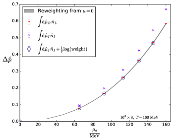
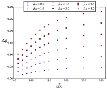
Figure 1: Left panel: The pressure difference between the zero and finite chemical potential theory calculated with several different reweighting methods as a function of the quark chemical potential at $T=160$ MeV. Results at finite isospin chemical potential are shown as purple points. Results reweighted from the phase quenched ensemble to finite baryon density with the two methods discussed in the text are shown by red and blue points. Results from reweighting from zero chemical potential are shown in grey. Right panel: The pressure difference between zero and non-zero baryochemical potentials, calculated with phase reweighting as a function of the temperature, for different fixed values of $\hat{\mu}$.

Observables

The grand canonical partition function of lattice QCD is given schematically by:

$$Z(T,\mu)=\int\mathcal{D}U\,\det{\textrm{M}}(U,\mu)e^{-S_{g}(U)}\,,$$ (1)

where $S_{g}(U)$ is the gauge action, $\det\rm{M}$ is the quark determinant, implicitly including all flavors, as well as staggered rooting, $\mu$ collectively denotes the chemical potentials of all quark flavors and $U$ are the link variables. We work with the quark chemical potentials satisfying $\mu_{q}\equiv\mu_{u}=\mu_{d}$ and $\mu_{s}=0$. We concentrate on the pressure as a function of the temperature and dimensionless chemical potential $\hat{\mu}_{B}\equiv\mu_{B}/T=3\mu_{q}/T\equiv 3\hat{\mu}_{q}$ , given by

$$\hat{p}(T,\hat{\mu}_{B})\equiv\frac{p(T,\hat{\mu}_{B})}{T^{4}}=\frac{1}{\left(LT\right)^{3}}\ln Z(T,\hat{\mu}_{B})\rm{.}$$ (2)

In particular, we study the pressure difference between zero and non-zero chemical potentials:

$$\Delta\hat{p}=\frac{\Delta p}{T^{4}}\equiv\hat{p}(T,\hat{\mu}_{B})-\hat{p}(T,0)\rm{.}$$ (3)

We also compute the light quark density:

$$\hat{n}_{L}\left(T,\hat{\mu}_{B}\right) \equiv\frac{{\rm{d}}\hat{p}}{{\rm{d}}\hat{\mu}_{B}}=\frac{1}{3\left(LT\right)^{3}}\left(\frac{\partial\ln Z(T,\hat{\mu}_{B})}{\partial\hat{\mu}_{q}}\right)_{\mu_{s}=0}\rm{.}$$ (4)

The integral of $\hat{n}_{L}$ over $\hat{\mu}_{B}$ is $\Delta\hat{p}$. We calculate the equation of state with several different methods.

Reweighting from $\mu_{B}=0$

In what is arguably the simplest reweighting scheme, simulations are performed at $\mu_{B}=0$ and $\Delta\hat{p}$ is reconstructed via [47]:

$$\Delta\hat{p}(T,\hat{\mu}_{B})=\frac{1}{\left(LT\right)^{3}}\ln\left\langle\frac{\det\rm{M}(\hat{\mu}_{B})}{\det\rm{M}(0)}\right\rangle_{\hat{\mu}_{B}=0}\rm{.}$$ (5)

While Eq. (5) is exact with infinite statistics, the tails of the distribution of the weights $\frac{\det{\rm{M}}(\hat{\mu}_{B})}{\det{\rm{M}}(0)}$ are heavy and so hard to sample correctly (overlap problem), and it is therefore hard to judge the reliability of results obtained with this method. It was proposed that the overlap problem can be mitigated by reweighting in more parameters [48, 49, 50]. However, even with multi-parameter reweighting, the overlap problem remains the main bottleneck of the method (at least around the transition line, where this question was studied in Ref.  [51]). We include results from (one-parameter) reweighting from $\mu_{B}=0$ for completeness, and also because one of the resummation strategies we are going to test can be regarded as a truncation of this reweighting scheme.

Phase reweighting

A way to avoid heavy-tailed distributions in the weights is to simulate a theory where these can only take values in a compact domain. Two examples are sign reweighting [52, 53, 39, 40] and phase reweighting [54, 55, 40]. Here we use the latter. Here in the simulated theory one replaces the quark determinant with its absolute value. The simulated ensemble is called the phase quenched ensemble, corresponding to a finite isospin chemical potential, i.e., $\mu_{u}=-\mu_{d}$. The pressure then schematically reads:

$$\hat{p}_{I}(T,\hat{\mu}_{q})=\frac{1}{\left(LT\right)^{3}}\log\int\mathcal{D}U\left|\det{\rm{M}}\right|e^{-S_{g}}\rm{.}$$ (6)

It is also given by the integral of the isospin density:

$$\hat{n}_{I}(T,\hat{\mu}_{q})\equiv\left(\frac{\partial\hat{p}_{I}}{\partial\hat{\mu_{q}}}\right)_{\mu_{s}=0}$$ (7)

from which the pressure at finite $\mu_{B}$ is obtained as:

$$\hat{p}(T,\hat{\mu}_{B}=3\hat{\mu}_{q})-\hat{p}_{I}(T,\hat{\mu}_{q})=\frac{1}{\left(LT\right)^{3}}\ln\left\langle e^{i\theta}\right\rangle_{PQ}\rm{,}$$ (8)

where $e^{i\theta}=\frac{\det{\rm{M}}(\hat{\mu}_{B})}{\left|\det{\rm{M}}(\hat{\mu}_{B})\right|}$ is the complex phase factor of the fermion determinant and $\left\langle\dots\right\rangle_{PQ}$ means taking an expectation value in the phase quenched theory. One finally arrives at:

$$\Delta\hat{p}=\int_{0}^{\hat{\mu}_{B}/3}\hat{n}_{I}(\hat{\mu}_{q},T){\rm{d}}\hat{\mu}_{q}+\frac{1}{\left(LT\right)^{3}}\ln\left\langle e^{i\theta}\right\rangle_{PQ}\rm{.}$$ (9)

Alternatively, one can calculate $\hat{n}_{L}$ directly with reweighting:

$$\hat{n}_{L}=\frac{1}{\left(LT\right)^{3}\left\langle e^{i\theta}\right\rangle_{PQ}}\left\langle e^{i\theta}\frac{\partial}{\partial\hat{\mu}_{B}}\ln\det\rm{M}\right\rangle_{PQ}\rm{,}$$ (10)

from which the pressure difference can be calculated via integration. The two methods are not a priori guaranteed to give the same results if the observable in the numerator of Eq. (10), namely $e^{i\theta}\frac{\partial}{\partial\hat{\mu}_{B}}\ln\det\rm{M}$, has an overlap problem. In principle this could happen, as only the pressure difference $p(T,\hat{\mu}_{B}=\hat{\mu}_{q})-p_{I}(T,\hat{\mu}_{I}=\hat{\mu}_{q})\propto\left\langle e^{i\theta}\right\rangle_{PQ}$ in Eq. (8) is guaranteed to be free of one - due to the compactness of the observable $e^{i\theta}$.

The phase diagram at finite isospin density was calculated in Ref. [45]. The phase quenched ensemble has a pion condensed phase for low $T$ and $\mu_{q}>m_{\pi}/2$. In this region, the sign problem is expected to be severe. Here we avoid this issue since we concentrate on the equation of state of the QGP, and we find a mild sign problem: $\left\langle e^{i\theta}\right\rangle_{PQ}=\left\langle\cos\theta\right\rangle_{PQ}$ never gets below $0.1$ in any of our ensembles and is always more than $10\sigma$ away from zero.

Taylor expansion

The pressure is expanded in powers of the baryochemical potential:

$$\hat{p}(T,\hat{\mu}_{B})=p_{0}\left(T\right)+p_{2}\left(T\right)\hat{\mu}_{B}^{2}+p_{4}\left(T\right)\hat{\mu}_{B}^{4}+\dots\,.$$ (11)

We calculate the Taylor expansion coefficients in two different ways: by using configurations generated at $\mu_{B}=0$ to calculate them directly, and by using simulations at imaginary chemical potentials to obtain them from a fit. These are the two procedures used in the literature so far. For a recent example of the first method see, e.g., Ref. [17], for the second one Refs. [26, 31]. More details on the determination of the coefficients are given in the section on our numerical results.

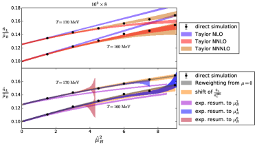
Figure 2: The direct results for $\hat{n}_{L}$ at non-zero $\mu_{B}$ compared with different approximations (or extrapolations): the Taylor method to different orders up to $p_{8}$ and the exponential resummations [35] to order $N=2,4$ and $6$, calculated from the ensemble at $\mu_{B}=0$, as well as the shifting $n_{L}/n_{L}^{\rm{SBL}}$ method calculated from imaginary chemical potential simulations and reweighting from $\mu_{B}=0$.

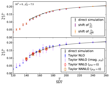
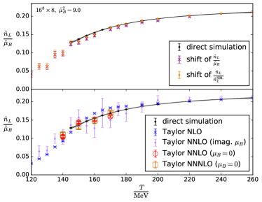
Figure 3: The density $\hat{n}_{L}$ as a function of the temperature $T$ for $\hat{\mu}_{B}=\sqrt{7.5}$ (left) and $\hat{\mu}_{B}=3$ (right) for the ordinary Taylor expansion (bottom) and the resummation schemes based on shifting $\hat{n}_{L}/\hat{\mu}_{B}$ and $\hat{n}_{L}/\hat{n}_{L}^{\rm{SBL}}$ (top). The direct Taylor data from $\mu_{B}=0$ simulations has smaller errors than the fit to imaginary $\mu_{B}$ data. This is mainly due to the small volume in our study. For larger volumes, the signal-to-noise ratio of the direct $p_{6}$ and $p_{8}$ would be considerably larger. A spline interpolation of the direct results is included to lead the eye.

Resummations based on shifting sigmoid functions

A resummation of the Taylor expansion was introduced in Ref. [34], defined by the implicit equation

$$\frac{\hat{n}_{L}\left(T,\hat{\mu}_{B}\right)}{\hat{\mu}_{B}}=\frac{{\rm{d}}\hat{n}_{L}}{{\rm{d}}\hat{\mu}_{B}}\left(T\left(1+\kappa_{2}\left(T\right)\hat{\mu}_{B}^{2}+\dots\right),0\right)\rm{.}$$ (12)

This is motivated by the empirical observation of the existence of an approximate scaling variable $T(1+\kappa\hat{\mu}_{B}^{2})$, coming from lattice studies at imaginary chemical potential. These show that certain observables collapse on single (sigmoid shaped) curves when plotted against this variable [33, 34]. Up to $\hat{\mu}_{B}=1.5$ the existence of an approximate scaling variable has also been confirmed directly at a real $\mu_{B}$ by reweighting from the sign quenched ensemble [40]. We call this the $\frac{\hat{n}_{L}\left(T,\hat{\mu}_{B}\right)}{\hat{\mu}_{B}}$ shifting method. This is a systematically improvable expansion. Its validity is not predicated on the existence of this approximate scaling variable, only its fast convergence: i.e., if an approximate scaling variable exists, we expect the method to converge fast.

A disadvantage of the previous scheme is that it was designed to work only near the crossover. To make it more suitable for high $T$, it was later refined [38] by introducing a Stefan-Boltzmann correction:

$$\frac{\hat{n}_{L}\left(T,\hat{\mu}_{B}\right)}{\hat{n}_{L}^{\rm{SBL}}\left(\hat{\mu}_{B}\right)}=\lim_{\hat{\mu}_{B}^{\prime}\to 0}\frac{\hat{n}_{L}\left(T\left(1+\lambda_{2}\hat{\mu}_{B}^{2}+\dots\right),\hat{\mu}_{B}^{\prime}\right)}{\hat{n}_{L}^{\rm{SBL}}\left(\hat{\mu}_{B}^{\prime}\right)}\rm{,}$$ (13)

where we introduced the Stefan-Boltzmann limit:

$$\hat{n}_{L}^{\rm{SBL}}(\hat{\mu}_{B})\equiv\lim_{T\to\infty}\hat{n}_{L}(T,\hat{\mu}_{B})\rm{.}$$ (14)

We call this method the $\frac{\hat{n}_{L}\left(T,\hat{\mu}_{B}\right)}{\hat{n}_{L}^{\rm{SBL}}}$ shifting method. Both shifting methods can be implemented by fitting the $\kappa_{n}$ or $\lambda_{n}$ coefficients to data at imaginary $\mu_{B}$.

Exponential resummation

A different resummation is based on truncating the reweighting from $\mu_{B}=0$ [35], by approximating $\frac{\det\rm{M}(\hat{\mu}_{B})}{\det\rm{M}(0)}\simeq\exp\left(\sum_{n=1}^{N}\frac{1}{n!}\mathcal{D}_{n}\hat{\mu}_{B}^{n}\right)$ in Eq. (5):

$$\Delta\hat{p}(T,\hat{\mu}_{B})\simeq\frac{1}{\left(LT\right)^{3}}\ln\left\langle\exp\left(\sum_{n=1}^{N}\frac{1}{n!}\mathcal{D}_{n}\hat{\mu}_{B}^{n}\right)\right\rangle_{\hat{\mu}_{B}=0}\rm{,}$$ (15)

where $\mathcal{D}_{n}\equiv\frac{\partial^{n}}{\partial\hat{\mu}_{B}^{2}}\ln\det\rm{M(\hat{\mu}_{B})}$ and $N$ is the truncation order. This method could either be called truncated reweighting or an exponential resummation of the Taylor series. A practical advantage of this scheme is that the coefficients $\mathcal{D}_{n}$ are needed for the calculation of the Taylor expansion coefficients $p_{2n}$ anyway. Thus, this resummation scheme represents an alternative way to analyze lattice data for the Taylor coefficients. The procedure introduced in Ref. [35] had the disadvantage of using a biased estimator for the expectation value in Eq. (15), by simply exponentiating the stochastic estimators of the $\mathcal{D}_{n}$. This bias was studied in Ref. [36]. We remove this bias by calculating the $\mathcal{D}_{n}$ exactly for each configuration, using the reduced matrix formalism [56]. Note that unlike the Taylor expansion or the resummations based on shifting sigmoids, this scheme is not defined in terms of thermodynamic quantities, but by an approximation of the integrand of the path integral. Thus, the convergence properties of the scheme are not guaranteed to be governed by the analytic properties of the free energy.

Lattice setup and numerical results

We used a tree-level Symanzik improved gauge action, and two steps of stout smearing [57] with a smearing parameter $\rho=0.15$ on the gauge links entering the quark determinant, with physical quark masses, using the kaon decay constant $f_{K}$ for scale setting (see Ref. [58] for details). We apply a tree-level improvement factor to the pressure, that makes the $N_{\tau}=8$ 2stout results already close to the continuum [5]. This corresponds to division by $1.28$ at infinite volume, which is the correction we apply for $\hat{n}_{L}$ and $\Delta\hat{p}$.

We study $16^{3}\times 8$ lattices at various temperatures in the range $145$ MeV $\leq T\leq 240$ MeV and light-quark chemical potential $\mu_{u}=\mu_{d}=\mu_{q}=\mu=\mu_{B}/3$ with a zero strange quark chemical potential $\mu_{s}=0$, corresponding to a strangeness chemical potential $\mu_{S}=\mu_{B}/3$.

We simulate the phase quenched ensemble for $\hat{\mu}_{B}^{2}=1.5,3,4.5,6,7.5$ and $9$. These simulations are performed without an explicit symmetry breaking term, commonly used in simulations at a finite isospin density [59, 45]. Instead, we follow the method of Ref. [40]. The resulting ensemble corresponds to an isospin chemical potential $\mu_{I}=\mu_{u}=-\mu_{d}$. We use these ensembles to reweight to a baryochemical potential with $\mu_{u}=\mu_{d}=\mu_{B}/3$. Determinant ratios are calculated using the reduced matrix formalism [56, 60]. We performed the calculation of $\Delta\hat{p}$ in the two inequivalent ways: the one with no possible overlap problem described by Eq. (9), and by integration of Eq. (10). We obtain compatible results for $\Delta\hat{p}$ with the two methods, as can be seen in Fig. 1 (left) for $T=160$ MeV.

We also simulate at $\mu_{B}=0$ for four temperatures: $T/{\rm{MeV}}=140,150,160$ and $170$. This is to perform reweighting from $\mu_{B}=0$, to calculate the Taylor expansion coefficients, and to perform the exponential resummation. For all of these, we used the reduced matrix formalism of Ref. [56], so obtaining the Taylor coefficients without the use of stochastic estimators and obtaining $\mathcal{D}_{n}$ exactly for each configuration, and encountering no bias in the exponential resummation [35, 36].

In Fig. 1 (left) we also show the results for $\Delta\hat{p}$ from reweighting from $\mu_{B}=0$. These results are again in perfect agreement with the two different ways of reweighting from the phase quenched ensemble. This is true for all temperatures in our study.

Thus, three different reweighting procedures - including one with no possible overlap problem - give identical results. This strongly supports the validity of our results for the equation of state. The full set of results for $\Delta\hat{p}$ from phase reweighting are shown in Fig. 1 (right). We can safely use these results to test extrapolation schemes.

Without comparison with the phase reweighted results, we would have no way to guarantee the correctness of reweighting from $\mu_{B}=0$, due to the uncontrolled systematics of the overlap problem. This problem is also present in the Taylor method, since for a finite ensemble the Taylor coefficients necessarily correspond to the Taylor coefficients of the pressure one would have obtained by reweighting from $\mu_{B}=0$. By first showing that reweighting from $\mu_{B}=0$ works for the region $\hat{\mu}_{B}\leq 3$, we ensure that we are truly testing the convergence properties of the Taylor series, without being limited by an overlap problem in the higher order coefficients.

Comparison with extrapolation schemes

To implement the resummation schemes based on shifting sigmoids, we perform simulations at imaginary chemical potentials, for $\operatorname{Im}\hat{\mu}_{B}\frac{16}{\pi}=0,4,6,7,8,9,10$ and $12$. We work to order $\kappa_{4}$ in Eq. (12) and to order $\lambda_{4}$ in Eq. (13), using a simplified version of the analysis of Refs. [34, 38]. The systematic error includes the fit range in imaginary $\mu_{B}$, the ansatz in $\mu_{B}^{2}$, and the interpolation of the light quark susceptibility at $\mu_{B}=0$. We also demonstrate a more straightforward use of the imaginary chemical potential data by performing a second determination of the Taylor expansion coefficients, fitting $\frac{\hat{n}_{L}}{\hat{\mu}_{B}}$ with a polynomial of order $\hat{\mu}_{B}^{6}$. For the fits we also include $\frac{d^{2}\hat{p}}{d\hat{\mu}_{B}^{2}}$ and $\frac{d^{4}\hat{p}}{d\hat{\mu}_{B}^{4}}$ at $\mu_{B}=0$ as further datapoints.

We show the comparison of the different reweighting schemes with the direct data in Fig. 3, as a function of the chemical potential at fixed temperatures of $T=160$ MeV and $170$ MeV, and in Fig. 2, as a function of $T$ at a fixed $\hat{\mu}_{B}=\sqrt{7.5}$ and $3$ - the two largest values where we have direct data. The Taylor expansion at next-to-leading order - $\mathcal{O}(\mu_{B}^{4})$ in the pressure - is not consistent with the direct data, systematically underestimating $n_{L}$ below $150$ MeV, and systematically overestimating it above $150$ MeV. This is due to a peak in $p_{4}(T)$ slightly above the crossover temperature. Including the next term in the expansion, with the coefficient $p_{6}(T)$, the Taylor method agrees with the direct data up to $\hat{\mu}_{B}=3$ at $T=160$ MeV and up to $\hat{\mu}_{B}\approx 1.2$ at $T=170$ MeV. Including the next-to-next-to-next-to-leading order term $p_{8}(T)$, the expansion agrees with the direct data at all studied temperatures up to $\hat{\mu}_{B}=3$.

In contrast, the exponential resummation scheme shows bad convergence properties from $\hat{\mu}_{B}^{2}\approx 4$ for all temperatures. While the $N=2$ truncation of the scheme remains close to the direct results in the entire range, the higher orders make the agreement better only below this value, but not above.

At large $T$, the method based on shifting $\hat{n}_{L}/\hat{n}_{L}^{\rm{SBL}}$ outperforms the method of shifting $\hat{n}_{L}/\hat{\mu}_{B}$. This is not surprising, as the Stefan-Boltzmann correction was introduced in Ref. [38] as a way to improve the convergence properties of the scheme at high $T$.

In summary, we can say that both the Taylor expansion to order $\hat{\mu}_{B}^{8}$ and the resummation based on shifting $\hat{n}_{L}/\hat{n}_{L}^{\rm{SBL}}$ to order $\lambda_{4}$ accurately describe the direct data for the equation of state in the range $0\leq\hat{\mu}_{B}\leq 3$ - which includes the entire range of the RHIC Beam Energy Scan. Note the faster convergence of the resummed expansion, as the calculation of the coefficient $\lambda_{4}$ only requires the determination of the Taylor coefficients up to order $\hat{\mu}_{B}^{6}$. On the other hand, the shifting $\hat{n}_{L}/\hat{\mu}_{B}$ method at order $\kappa_{4}$ has a slight systematic discrepancy with the direct data at large $T$, and exponential resummation shows bad convergence properties in $N$ above $\hat{\mu}_{B}^{2}\approx 4$.

Outlook

We judged the reliability of different approximation schemes by comparing them with direct non-zero chemical potential results in the range $0\leq\hat{\mu}_{B}\leq 3$. While this gives a practical answer to the question of which approximation one can trust, a theoretical understanding of the reasons would also be welcome. For the schemes defined purely in terms of thermodynamic quantities, such as the Taylor expansion or the resummations based on shifting sigmoids, this requires knowledge of the position of partition function (Lee-Yang) zeros in the complex $\mu_{B}$ plane [16, 60, 61, 62, 37]. The exponential resummation scheme, instead, is not defined in terms of thermodynamic quantities, but comes rather from manipulating the integrand of the path integral for the partition function. Understanding its convergence region might also require better understanding of the nuances of the path integral, in addition to the thermodynamic singularities. We speculate that the limited convergence region has to do with quark determinant zeros. In fact, the sum appearing as the argument of the exponential in Eq. (15) approximates the effective action of the quarks in a fixed gauge field background, with a radius of convergence determined by the determinant zeros, which correspond to logarithmic divergences of the effective action. These are not simply related to the Lee-Yang zeros of the partition function, and may provide stronger limitations on the convergence of the expansion.

An obvious challenge is to extend the range of validity of the methods studied in this paper to lower $T$ and higher $\hat{\mu}_{B}$, so that the transition line [30, 15, 33, 63, 64], and the location of the conjectured critical endpoint [65, 66, 67, 68, 69] can be studied with first principle lattice calculations. Of course, the continuum and infinite volume limits will also have to be taken eventually.

References

- Montvay and Münster [1997] I. Montvay and G. Münster, Quantum fields on a lattice, Cambridge Monographs on Mathematical Physics (Cambridge University Press, 1997).
- Aoki et al. [2006a] Y. Aoki, G. Endrődi, Z. Fodor, S. D. Katz, and K. K. Szabó, Nature 443, 675 (2006a), arXiv:hep-lat/0611014 .
- Borsányi et al. [2010] S. Borsányi, Z. Fodor, C. Hoelbling, S. D. Katz, S. Krieg, C. Ratti, and K. K. Szabó (Wuppertal-Budapest), JHEP 09, 073, arXiv:1005.3508 [hep-lat] .
- Bazavov et al. [2012] A. Bazavov et al., Phys. Rev. D 85, 054503 (2012), arXiv:1111.1710 [hep-lat] .
- Borsányi et al. [2010] S. Borsányi, G. Endrődi, Z. Fodor, A. Jakovác, S. D. Katz, S. Krieg, C. Ratti, and K. K. Szabó, JHEP 11, 077, arXiv:1007.2580 [hep-lat] .
- Bazavov et al. [2014] A. Bazavov et al. (HotQCD), Phys. Rev. D 90, 094503 (2014), arXiv:1407.6387 [hep-lat] .
- Gavai and Gupta [2003] R. V. Gavai and S. Gupta, Phys. Rev. D 68, 034506 (2003), arXiv:hep-lat/0303013 .
- Allton et al. [2005] C. R. Allton, M. Doring, S. Ejiri, S. J. Hands, O. Kaczmarek, F. Karsch, E. Laermann, and K. Redlich, Phys. Rev. D 71, 054508 (2005), arXiv:hep-lat/0501030 [hep-lat] .
- Basak et al. [2008] S. Basak et al. (MILC), PoS LATTICE2008, 171 (2008), arXiv:0910.0276 [hep-lat] .
- Borsányi et al. [2012a] S. Borsányi, Z. Fodor, S. D. Katz, S. Krieg, C. Ratti, and K. Szabó, JHEP 01, 138, arXiv:1112.4416 [hep-lat] .
- Borsányi et al. [2012b] S. Borsányi, G. Endrődi, Z. Fodor, S. Katz, S. Krieg, et al., JHEP 08, 053, arXiv:1204.6710 [hep-lat] .
- Bellwied et al. [2015a] R. Bellwied, S. Borsányi, Z. Fodor, S. D. Katz, A. Pásztor, C. Ratti, and K. K. Szabó, Phys. Rev. D 92, 114505 (2015a), arXiv:1507.04627 [hep-lat] .
- Ding et al. [2015] H. T. Ding, S. Mukherjee, H. Ohno, P. Petreczky, and H. P. Schadler, Phys. Rev. D 92, 074043 (2015), arXiv:1507.06637 [hep-lat] .
- Bazavov et al. [2017] A. Bazavov et al., Phys. Rev. D 95, 054504 (2017), arXiv:1701.04325 [hep-lat] .
- Bazavov et al. [2019] A. Bazavov et al. (HotQCD), Phys. Lett. B 795, 15 (2019), arXiv:1812.08235 [hep-lat] .
- Giordano and Pásztor [2019] M. Giordano and A. Pásztor, Phys. Rev. D 99, 114510 (2019), arXiv:1904.01974 [hep-lat] .
- Bazavov et al. [2020] A. Bazavov et al., Phys. Rev. D 101, 074502 (2020), arXiv:2001.08530 [hep-lat] .
- de Forcrand and Philipsen [2002] P. de Forcrand and O. Philipsen, Nucl. Phys. B 642, 290 (2002), arXiv:hep-lat/0205016 [hep-lat] .
- D’Elia and Lombardo [2003] M. D’Elia and M. P. Lombardo, Phys. Rev. D 67, 014505 (2003), arXiv:hep-lat/0209146 [hep-lat] .
- D’Elia and Sanfilippo [2009] M. D’Elia and F. Sanfilippo, Phys. Rev. D 80, 014502 (2009), arXiv:0904.1400 [hep-lat] .
- Cea et al. [2014] P. Cea, L. Cosmai, and A. Papa, Phys. Rev. D 89, 074512 (2014), arXiv:1403.0821 [hep-lat] .
- Bonati et al. [2014] C. Bonati, P. de Forcrand, M. D’Elia, O. Philipsen, and F. Sanfilippo, Phys. Rev. D 90, 074030 (2014), arXiv:1408.5086 [hep-lat] .
- Cea et al. [2016] P. Cea, L. Cosmai, and A. Papa, Phys. Rev. D 93, 014507 (2016), arXiv:1508.07599 [hep-lat] .
- Bonati et al. [2015] C. Bonati, M. D’Elia, M. Mariti, M. Mesiti, F. Negro, and F. Sanfilippo, Phys. Rev. D 92, 054503 (2015), arXiv:1507.03571 [hep-lat] .
- Bellwied et al. [2015b] R. Bellwied, S. Borsányi, Z. Fodor, J. Günther, S. D. Katz, C. Ratti, and K. K. Szabó, Phys. Lett. B 751, 559 (2015b), arXiv:1507.07510 [hep-lat] .
- D’Elia et al. [2017] M. D’Elia, G. Gagliardi, and F. Sanfilippo, Phys. Rev. D 95, 094503 (2017), arXiv:1611.08285 [hep-lat] .
- Günther et al. [2017] J. N. Günther, R. Bellwied, S. Borsányi, Z. Fodor, S. D. Katz, A. Pásztor, C. Ratti, and K. K. Szabó, Proceedings, 26th International Conference on Ultra-relativistic Nucleus-Nucleus Collisions (Quark Matter 2017): Chicago, Illinois, USA, February 5-11, 2017, Nucl. Phys. A967, 720 (2017), arXiv:1607.02493 [hep-lat] .
- Alba et al. [2017] P. Alba et al., Phys. Rev. D 96, 034517 (2017), arXiv:1702.01113 [hep-lat] .
- Vovchenko et al. [2017] V. Vovchenko, A. Pásztor, Z. Fodor, S. D. Katz, and H. Stoecker, Phys. Lett. B 775, 71 (2017), arXiv:1708.02852 [hep-ph] .
- Bonati et al. [2018] C. Bonati, M. D’Elia, F. Negro, F. Sanfilippo, and K. Zambello, Phys. Rev. D 98, 054510 (2018), arXiv:1805.02960 [hep-lat] .
- Borsányi et al. [2018] S. Borsányi, Z. Fodor, J. N. Günther, S. K. Katz, K. K. Szabó, A. Pásztor, I. Portillo, and C. Ratti, JHEP 10, 205, arXiv:1805.04445 [hep-lat] .
- Bellwied et al. [2020] R. Bellwied, S. Borsányi, Z. Fodor, J. N. Günther, J. Noronha-Hostler, P. Parotto, A. Pásztor, C. Ratti, and J. M. Stafford, Phys. Rev. D 101, 034506 (2020), arXiv:1910.14592 [hep-lat] .
- Borsányi et al. [2020] S. Borsányi, Z. Fodor, J. N. Günther, R. Kara, S. D. Katz, P. Parotto, A. Pásztor, C. Ratti, and K. K. Szabó, Phys. Rev. Lett. 125, 052001 (2020), arXiv:2002.02821 [hep-lat] .
- Borsányi et al. [2021] S. Borsányi, Z. Fodor, J. N. Günther, R. Kara, S. D. Katz, P. Parotto, A. Pásztor, C. Ratti, and K. K. Szabó, Phys. Rev. Lett. 126, 232001 (2021), arXiv:2102.06660 [hep-lat] .
- Mondal et al. [2022] S. Mondal, S. Mukherjee, and P. Hegde, Phys. Rev. Lett. 128, 022001 (2022), arXiv:2106.03165 [hep-lat] .
- Mitra et al. [2022] S. Mitra, P. Hegde, and C. Schmidt, (2022), arXiv:2205.08517 [hep-lat] .
- Bollweg et al. [2022] D. Bollweg, J. Goswami, O. Kaczmarek, F. Karsch, S. Mukherjee, P. Petreczky, C. Schmidt, and P. Scior (HotQCD), Phys. Rev. D 105, 074511 (2022), arXiv:2202.09184 [hep-lat] .
- Borsanyi et al. [2022a] S. Borsanyi, Z. Fodor, J. N. Guenther, R. Kara, P. Parotto, A. Pasztor, C. Ratti, and K. K. Szabo, Phys. Rev. D 105, 114504 (2022a), arXiv:2202.05574 [hep-lat] .
- Giordano et al. [2020a] M. Giordano, K. Kapás, S. D. Katz, D. Nógrádi, and A. Pásztor, JHEP 05, 088, arXiv:2004.10800 [hep-lat] .
- Borsanyi et al. [2022b] S. Borsanyi, Z. Fodor, M. Giordano, S. D. Katz, D. Nogradi, A. Pasztor, and C. H. Wong, Phys. Rev. D 105, L051506 (2022b), arXiv:2108.09213 [hep-lat] .
- Aoki et al. [2006b] Y. Aoki, Z. Fodor, S. D. Katz, and K. K. Szabó, Phys. Lett. B 643, 46 (2006b), arXiv:hep-lat/0609068 .
- Bali et al. [2012a] G. S. Bali, F. Bruckmann, G. Endrődi, Z. Fodor, S. D. Katz, S. Krieg, A. Schäfer, and K. K. Szabó, JHEP 02, 044, arXiv:1111.4956 [hep-lat] .
- Bali et al. [2012b] G. S. Bali, F. Bruckmann, G. Endrődi, Z. Fodor, S. D. Katz, and A. Schäfer, Phys. Rev. D 86, 071502 (2012b), arXiv:1206.4205 [hep-lat] .
- Borsányi et al. [2015] S. Borsányi, Z. Fodor, S. D. Katz, A. Pásztor, K. K. Szabó, and C. Török, JHEP 04, 138, arXiv:1501.02173 [hep-lat] .
- Brandt et al. [2018] B. B. Brandt, G. Endrődi, and S. Schmalzbauer, Phys. Rev. D 97, 054514 (2018), arXiv:1712.08190 [hep-lat] .
- D’Elia et al. [2019] M. D’Elia, F. Negro, A. Rucci, and F. Sanfilippo, Phys. Rev. D 100, 054504 (2019), arXiv:1907.09461 [hep-lat] .
- Barbour et al. [1998] I. M. Barbour, S. E. Morrison, E. G. Klepfish, J. B. Kogut, and M.-P. Lombardo, Nucl. Phys. B Proc. Suppl. 60, 220 (1998), arXiv:hep-lat/9705042 .
- Fodor and Katz [2002a] Z. Fodor and S. D. Katz, Phys. Lett. B 534, 87 (2002a), arXiv:hep-lat/0104001 .
- Fodor and Katz [2002b] Z. Fodor and S. D. Katz, JHEP 03, 014, arXiv:hep-lat/0106002 .
- Fodor and Katz [2004] Z. Fodor and S. D. Katz, JHEP 04, 050, arXiv:hep-lat/0402006 .
- Giordano et al. [2020b] M. Giordano, K. Kapas, S. D. Katz, D. Nogradi, and A. Pasztor, Phys. Rev. D 102, 034503 (2020b), arXiv:2003.04355 [hep-lat] .
- de Forcrand et al. [2003] P. de Forcrand, S. Kim, and T. Takaishi, Nucl. Phys. B Proc. Suppl. 119, 541 (2003), arXiv:hep-lat/0209126 .
- Alexandru et al. [2005] A. Alexandru, M. Faber, I. Horváth, and K.-F. Liu, Phys. Rev. D 72, 114513 (2005), arXiv:hep-lat/0507020 .
- Fodor et al. [2007] Z. Fodor, S. D. Katz, and C. Schmidt, JHEP 03, 121, arXiv:hep-lat/0701022 .
- Endrődi et al. [2018] G. Endrődi, Z. Fodor, S. D. Katz, D. Sexty, K. K. Szabó, and C. Török, Phys. Rev. D 98, 074508 (2018), arXiv:1807.08326 [hep-lat] .
- Hasenfratz and Toussaint [1992] A. Hasenfratz and D. Toussaint, Nucl. Phys. B 371, 539 (1992).
- Morningstar and Peardon [2004] C. Morningstar and M. J. Peardon, Phys. Rev. D 69, 054501 (2004), arXiv:hep-lat/0311018 .
- Aoki et al. [2009] Y. Aoki, S. Borsányi, S. Durr, Z. Fodor, S. D. Katz, S. Krieg, and K. K. Szabó, JHEP 06, 088, arXiv:0903.4155 [hep-lat] .
- Kogut and Sinclair [2002] J. B. Kogut and D. K. Sinclair, Phys. Rev. D 66, 034505 (2002), arXiv:hep-lat/0202028 .
- Giordano et al. [2020c] M. Giordano, K. Kapas, S. D. Katz, D. Nogradi, and A. Pasztor, Phys. Rev. D 101, 074511 (2020c), [Erratum: Phys.Rev.D 104, 119901 (2021)], arXiv:1911.00043 [hep-lat] .
- Mukherjee et al. [2022] S. Mukherjee, F. Rennecke, and V. V. Skokov, Phys. Rev. D 105, 014026 (2022), arXiv:2110.02241 [hep-ph] .
- Dimopoulos et al. [2022] P. Dimopoulos, L. Dini, F. Di Renzo, J. Goswami, G. Nicotra, C. Schmidt, S. Singh, K. Zambello, and F. Ziesché, Phys. Rev. D 105, 034513 (2022), arXiv:2110.15933 [hep-lat] .
- Pásztor et al. [2021] A. Pásztor, Z. Szép, and G. Markó, Phys. Rev. D 103, 034511 (2021), arXiv:2010.00394 [hep-lat] .
- Haque and Strickland [2021] N. Haque and M. Strickland, Phys. Rev. C 103, 031901 (2021), arXiv:2011.06938 [hep-ph] .
- Fukushima [2008] K. Fukushima, Phys. Rev. D 77, 114028 (2008), [Erratum: Phys.Rev.D 78, 039902 (2008)], arXiv:0803.3318 [hep-ph] .
- Kovács et al. [2016] P. Kovács, Z. Szép, and G. Wolf, Phys. Rev. D 93, 114014 (2016), arXiv:1601.05291 [hep-ph] .
- Isserstedt et al. [2019] P. Isserstedt, M. Buballa, C. S. Fischer, and P. J. Gunkel, Phys. Rev. D 100, 074011 (2019), arXiv:1906.11644 [hep-ph] .
- Gao and Pawlowski [2021] F. Gao and J. M. Pawlowski, Phys. Lett. B 820, 136584 (2021), arXiv:2010.13705 [hep-ph] .
- Bernhardt et al. [2021] J. Bernhardt, C. S. Fischer, P. Isserstedt, and B.-J. Schaefer, Phys. Rev. D 104, 074035 (2021), arXiv:2107.05504 [hep-ph] .