Haar Wavelets, Gradients and Approximate Total Variation Regularization

Abstract

We show how total variation regularization of images in arbitrary dimensions can be approximately performed by applying appropriate shrinkage to some Haar wavelets coefficients. The approach works directly on the wavelet coefficients and is therefore suited for the application on large volumes from computed tomography.

68Q25, 68R10, 68U05

1 Introduction

Modern imaging techniques produce larger and larger images which have to be processed and analyzed. This is particularly true in industrial computed tomography where huge datasets of $1\text{\,}\mathrm{TB}$ and more are generated on an almost routine basis by either scanning very large objects [10] or working with a very high resolution in the $\text{\,}\mathrm{\SIUnitSymbolMicro m}$ scale and below. Even on advanced customer computer hardware, such bigtures cannot be handled without substantial compression. A natural and almost self-suggesting approach for that purpose is to use wavelet methods which have been established over more than three decades meanwhile and can be very easily applied in any dimensionality by making use of tensor products. For two-dimensional images, wavelets have become part of the JPEG2000 standard, and they have also been applied successfully for the compression of tomographic volume data, cf. [2, 12].

To illustrate the type of objects that we are concerned with, we refer to the CT scan of Peruvian mummy owned by the Lindenmuseum in Stuttgart that was performed at the Fraunhofer IIS Development Center X-ray Technology (EZRT). The size of the data set is $970\text{\,}\mathrm{GB}$ and in order to handle and visualized it on consumer computer hardware, it has been reduced to about $30\text{\,}\mathrm{GB}$ by the wavelet compression method from [12].

 

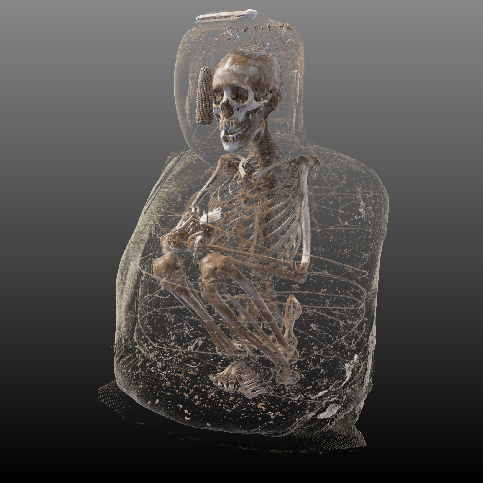
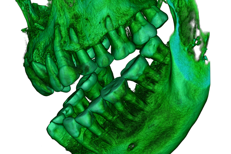
Figure 1: Rendering of the full mummy (left, courtesy of Fraunhofer MEVIS) and details of skull and teeth (right). All levels of detail in the latter rendering are obtained directly from the wavelet compression.

While high resolution parts of the scan can be obtained on the fly, the full resolution is not tractable with reasonable effort and this necessitates algorithms that work entirely on the wavelet coefficients.

The probably simplest choice for a wavelet is the Haar wavelet and the associated multiresolution analysis generated by characteristic functions of the unit interval and their dyadic refinement properties. Haar wavelets have the advantages of being compactly supported, orthonormal and symmetric, and they are the only wavelet system with these properties, cf. [6]. Moreover, Haar wavelets have minimal support among all discrete multiresolution systems and thus provide optimal localization. And, of course, they can be implemented in a very efficient way, allowing for fast decomposition and on-the-fly reconstruction of images. This by itself makes them interesting and useful despite their well-known drawbacks like lack of smoothness and vanishing moments.

On the other hand, the use of Haar wavelets can even be beneficial for more advanced problems, for example as a replacement for Fourier Analysis avoiding divergence phenomena in the original [3]. In this paper we show that and how Haar wavelets can be used for gradient estimation and an approximate total variation (TV) denoising, both working exclusively on the wavelet coefficients and without any need to reconstruct the full image. By this direct and computationally cheap manipulation of some wavelet coefficients, TV denoising can even be integrated into the visualization process in real time. The proofs will show that this is an intrinsic property of tensor product Haar wavelets: the fact that they do only provide one vanishing moment is responsible for their ability to approximate the gradient on a grid and their symmetry and explicit expression allow us to determine the explicit level-dependent renormalization coefficients that guarantee that direction and length of the gradients are met accurately.

The paper is organized as follows: in Section 3 we recall the definition of Haar wavelets, set up the notation for Haar wavelets in any number of variables and derive a saturation result for the wavelet coefficients depending on their type, more precisely, on the distribution of scaling and wavelet components in the tensor product function. Section 4 shows how the TV norm can of a function can be approximated by properly renormalized subset of wavelet coefficients and gives explicit error estimates for this approximation. How TV denoising based on the ROF functional can be done directly on the wavelet coefficients, is shown in Section 5. Finally, in Section 6 we give some example applications of the method on large CT data sets.

2 Related work

It has long been observed that soft thresholding of (especially Haar) wavelet coefficients is a useful tool for data denoising. A careful mathematical analysis and discussion of the relationship between Haar wavelet shrinkage and TV regularization has been given in [11] and [13], starting from the study of diffusion processes. More precisely, the authors showed that their diffusion-based process of denoising has strong connections to Haar wavelet shrinkage. Though this approach is superior to ours for the denoising of two dimensional images, it is not applicable to our needs as it relies on an iterative diffusion process of the complete image that is not practically feasible for gigavoxel datasets. In contrast, our approach only approximated the TV norm regularization but does by directly shrinking the Haar wavelet coefficients.

The geometric meaning of Haar wavelet coefficients has also been used implicitly in [7] to determine similarity indices which are essentially based on the role of a subset of the Haar wavelet coefficients as approximations of gradient vectors. This indeed might be carried over to three dimensions and could be directly applied for quality measurements between voxel datasets.

3 Haar wavelets

To fix notation, we begin by recalling the well-known concept of tensor product Haar wavelets on $\mathbb{R}^{s}$, where $s$ stands for the number of variables. In one variable, the Haar wavelets are based on the scaling function $\psi_{0}$ and the wavelet $\psi_{1}$, defined as

(1) $$\psi_{0}:=\chi_{[0,1]},\qquad\psi:=\psi_{1}:=\chi_{[0,\frac{1}{2}]}-\chi_{[\frac{1}{2},1]},$$

cf. [5]. Since $\psi_{0,k}:=\psi_{0}(\cdot-k)$ and the normalized wavelets $\psi_{1,k}^{n}:=2^{n/2}\psi_{1}\left(2^{n}\cdot-k\right)$, $k\in\mathbb{Z}$, $n\in\mathbb{N}_{0}$, form an orthonormal basis of $L_{2}(\mathbb{R})$, any function $f\in L_{2}(\mathbb{R})$ can be expressed in terms of its scaling and wavelet coefficients

$$c_{k}(f):=\int_{\mathbb{R}}f(t)\psi_{0}(t-k)\,dt,\quad d_{k}^{n}(f):=2^{n/2}\int_{\mathbb{R}}f(t)\psi_{1}(2^{n}t-k)\,dt,\qquad k\in\mathbb{Z},\,n\in\mathbb{N}_{0},$$

as

(2) $$f=\sum_{k\in\mathbb{Z}}c_{k}(f)\,\psi_{0,k}+\sum_{n=0}^{\infty}\sum_{k\in\mathbb{Z}}d_{k}^{n}(f)\,\psi_{1,k}^{n},$$

and the wavelet coefficients of different levels give rise to a multiresolution analysis.

The extension to $s$ variables by means of tensor product is straightforward. The index for a basis function is $\theta\in\{0,1\}^{s}$ and we define, for $x=(x_{1},\dots,x_{s})\in\mathbb{R}^{s}$,

(3) $$\psi_{\theta}(x):=\prod_{j=1}^{s}\psi_{\theta_{j}}(x_{j}),\qquad\theta\in\{0,1\}^{s}\setminus\{0\}.$$

We call $\psi_{0}=\chi_{[0,1]^{s}}$ the scaling function while all other functions $\psi_{\theta}$, $\theta\in\{0,1\}^{s}\setminus\{0\}$, are wavelets, giving $2^{s}-1$ wavelet functions at each level. With the scaling coefficients

$$c_{\alpha}(f)=\int_{\mathbb{R}^{s}}f(t)\psi_{0}(t-\alpha)\,dt,\qquad\alpha\in\mathbb{Z}^{s},$$

and the wavelet coefficients

$$d_{\theta,\alpha}^{n}(f)=2^{ns/2}\int_{\mathbb{R}^{s}}f(t)\psi_{\theta}(2^{n}t-\alpha)\,dt,\qquad\alpha\in\mathbb{Z}^{s},\,n\in\mathbb{N}_{0},$$

we obtain the orthogonal representation

(4) $$f=\sum_{\alpha\in\mathbb{Z}^{s}}c_{\alpha}(f)\,\psi_{0,\alpha}+\sum_{n=0}^{\infty}\sum_{\theta\neq 0}\sum_{\alpha\in\mathbb{Z}^{s}}d_{\theta,\alpha}^{n}(f)\,\psi_{\theta,\alpha}^{n},\qquad\psi_{\theta,\alpha}^{n}:=2^{ns/2}\psi_{\theta}(2^{n}\cdot-\alpha).$$

Of course, in applications one usually does not work with the infinite series, but only with a finite sum of wavelet levels up to some maximal level $n_{1}$.

3.1 Wavelet moments

As a first auxiliary result, we compute moments of the wavelets $\psi_{\theta}(\cdot-\alpha)$ relative to the polynomials $(\cdot+\frac{1}{2}\epsilon)^{\gamma}$, $|\gamma|\leq|\theta|$, where $\epsilon:=(1,\dots,1)\in\mathbb{Z}^{s}$; these polynomials are centered at the support of $\psi_{\theta}$. The scaled and shifted wavelets have the center of their support at the points

(5) $$x_{\alpha}^{n}:=2^{-n}\left(\alpha+\frac{1}{2}\epsilon\right).$$

Note that these points form a set of non-interlacing grids in $\mathbb{R}^{s}$. Indeed, if there were $n<n^{\prime}$ and $\alpha,\alpha^{\prime}\in\mathbb{Z}^{s}$ such that $x_{\alpha}^{n}=x_{\alpha^{\prime}}^{n^{\prime}}$, then this would mean that $2^{n^{\prime}-n}\left(\alpha+\frac{1}{2}\epsilon\right)=\alpha^{\prime}+\frac{1}{2}\epsilon$ which is impossible since the left hand side is a point in $\mathbb{Z}^{s}$ while the one on the right hand side lies in the shifted grid $\mathbb{Z}^{s}+\frac{1}{2}\epsilon$. The moments of monomials centered at such midpoints with respect to the Haar wavelets have a simple and explicit form which we record first.

Lemma 3.1.

For $\theta\in\{0,1\}^{s}$ and $|\gamma|\leq|\theta|$ one has

(6) $$\int_{\mathbb{R}^{s}}\left(x-x_{\alpha}^{n}\right)^{\gamma}\,\psi_{\theta,\alpha}^{n}(x)\,dx=(-1)^{|\theta|}2^{-(n+2)|\theta|-ns/2}\,\delta_{\gamma,\theta}.$$

Proof 3.2.

The integral in (6) can be written as

(7) $$\int_{\mathbb{R}^{s}}\left(x-x_{\alpha}^{n}\right)^{\gamma}\,\psi_{\theta,\alpha}^{n}(x)\,dx=\prod_{j=1}^{s}\int_{\mathbb{R}}\left(x_{j}-2^{-n}(\alpha_{j}+\frac{1}{2})\right)^{\gamma_{j}}\,\psi_{\theta_{j},\alpha_{j}}^{n}(x_{j})\,dx_{j}.$$

We first note that if $|\gamma|\leq|\theta|$ and $\gamma\neq\theta$ then there exists $k\in\{1,\dots,s\}$ such that $\gamma_{k}=0$ and $\theta_{k}=1$ and therefore

$$\int_{\mathbb{R}}\left(x_{j}-x_{\alpha}^{n}\right)^{0}\,\psi_{1,\alpha_{j}}^{n}(x_{j})\,dx_{j}=0,$$

hence, one factor in (7) vanishes and therefore the whole product. In consequence, the integral in (6) is nonzero only for $\gamma=\theta$. To compute the value of the integral, we note that by shift invariance we can restrict ourselves to the case $\alpha=0$. In the univariate case we note that

$$\int_{\mathbb{R}}\left(x-2^{-n-1}\right)^{0}\,\psi_{0,0}^{n}(x)\,dx=2^{n/2}\int_{\mathbb{R}}\psi_{0}(2^{n}x)\,dx=2^{-n/2},$$

as well as

$$\int_{\mathbb{R}}\left(x-2^{-n-1}\right)\,\psi_{1,0}^{n}(x)\,dx$$

$$= -2^{n/2}\left(\int_{0}^{2^{-n-1}}(2^{-n-1}-x)\,dx+\int_{2^{-n-1}}^{2^{-n}}\left(x-2^{-n-1}\right)\,dx\right)$$

$$= -2^{n/2}2^{-2n-2}=-2^{-\frac{3}{2}n-2},$$

so that the integral in (6) takes the value

$$\prod_{\theta_{j}=0}2^{-n/2}\,\prod_{\theta_{j}=1}\left(-2^{-\frac{3}{2}n-2}\right)=(-1)^{|\theta|}2^{-\frac{n}{2}(s-|\theta|)}\,2^{\left(-\frac{3}{2}n-2\right)|\theta|}=(-1)^{|\theta|}2^{-(n+2)|\theta|-ns/2}$$

whenever $\gamma=\theta$.

3.2 Limits of coefficients

The simple observation of Lemma 3.1 allows us to determine the limits of Haar wavelet coefficients for sufficiently smooth functions and their natural rate of decay.

Theorem 3.3.

For $\theta\in\{0,1\}^{s}$ suppose that $f\in C^{|\theta|+1}(\mathbb{R}^{s})$. Then,

(8) $$\lim_{n\to\infty}\left|(-1)^{|\theta|}2^{(n+2)|\theta|+ns/2}d_{\theta,\alpha}^{n}(f)-\frac{D^{\theta}f\left(x_{\alpha}^{n}\right)}{\theta!}\right|=0,\qquad\alpha\in\mathbb{Z}^{s}.$$

Proof 3.4.

For $n\in\mathbb{N}_{0}$ and $\alpha\in\mathbb{Z}^{s}$, we consider the $(|\theta|+1)$st Taylor expansion of $f$ at $x_{\alpha}$,

$$f(x)=\sum_{|\gamma|\leq|\theta|}\frac{D^{\gamma}f(x_{\alpha}^{n})}{\gamma!}\,\left(x-x_{\alpha}^{n}\right)+\sum_{|\gamma|=|\theta|+1}\frac{D^{\gamma}f(\xi)}{\gamma!}\left(x-x_{\alpha}^{n}\right)^{\gamma},\qquad x\in x_{\alpha}+\left[-\frac{1}{2},\frac{1}{2}\right]^{s}$$

where $\xi=\xi(x)\in x_{\alpha}+\left[-\frac{1}{2},\frac{1}{2}\right]^{s}$. Now, by Lemma 3.1,

$$d_{\theta,\alpha}^{n}(f)=\int_{\mathbb{R}^{s}}f(x)\,\psi_{\theta,\alpha}^{n}(x)\,dx$$

$$= (-1)^{|\theta|}2^{-(n+2)|\theta|-ns/2}\,\frac{D^{\theta}f(x_{\alpha}^{n})}{\theta!}$$

$$+\sum_{|\gamma|=|\theta|+1}\int_{\mathbb{R}^{s}}\frac{D^{\gamma}f\left(\xi(x)\right)}{\gamma!}\left(x-x_{\alpha}^{n}\right)^{\gamma}\,\psi_{\theta,\alpha}^{n}(x)\,dx.$$

The estimate

$$\left|\int_{\mathbb{R}^{s}}\frac{D^{\gamma}f\left(\xi(x)\right)}{\gamma!}\left(x-x_{\alpha}^{n}\right)^{\gamma}\,\psi_{\theta,\alpha}^{n}(x)\,dx\right|$$

$$\leq \max_{x\in x_{\alpha}+2^{-n}\left[-\frac{1}{2},\frac{1}{2}\right]^{s}}\left|\frac{D^{\gamma}f(x)}{\gamma!}\right|2^{n/2}\int_{x_{\alpha}+2^{-n}\left[-\frac{1}{2},\frac{1}{2}\right]^{s}}\left|x-x_{\alpha}\right|^{\gamma}\,dx$$

$$= 2^{-(n+1)(|\theta|+1)-ns/2}\max_{x\in x_{\alpha}+2^{-n}\left[-\frac{1}{2},\frac{1}{2}\right]^{s}}\left|\frac{D^{\gamma}f(x)}{\gamma!}\right|$$

holds for any $\gamma$ with $|\gamma|=|\theta|+1$ and immediately yields that

(9) $$\left|(-1)^{|\theta|}2^{(n+2)|\theta|+ns/2}d_{\theta,\alpha}^{n}(f)-\frac{D^{\theta}f\left(x_{\alpha}^{n}\right)}{\theta!}\right|$$

$$\leq {|\theta|+s\choose s-1}2^{|\theta|-n-1}\max_{|\gamma|=|\theta|+1}\max_{x\in x_{\alpha}+2^{-n}\left[-\frac{1}{2},\frac{1}{2}\right]^{s}}\left|\frac{D^{\gamma}f(x)}{\gamma!}\right|,$$

whose right hand side indeed tends to zero like $O(2^{-n})$ for $n\to\infty$.

If the $(|\theta|+1)$st derivative of $f$ is globally bounded in the sense that

$$\|D^{|\theta|+1}f\|_{\infty}:=\sup_{x\in\mathbb{R}^{s}}\max_{|\gamma|=|\theta|+1}\left|\frac{D^{\gamma}f(x)}{\gamma!}\right|<\infty,$$

then (9) holds independently of $\alpha$, and we get the following improvement of Theorem 3.3.

Corollary 3.5.

If $f\in C^{s+1}(\mathbb{R}^{s})$ and $\|D^{k}f\|_{\infty}<\infty$, $k=1,\dots,s+1$, then

(10) $$\lim_{n\to\infty}\sup_{\alpha\in\mathbb{Z}^{s}}\left|(-1)^{|\theta|}2^{(n+2)|\theta|+ns/2}d_{\theta,\alpha}^{n}(f)-\frac{D^{\theta}f\left(x_{\alpha}^{n}\right)}{\theta!}\right|=0,\qquad\theta\in\{0,1\}^{s}.$$

Theorem 3.3 and Corollary 3.5, respectively, have some consequences. The first is that Haar wavelet coefficients show what is known as a saturation behavior in Approximation Theory, cf. [4], i.e., they cannot decay faster than a given rate, namely $2^{-(n+2)|\theta|-ns/2}$, no matter how smooth the function is. Moreover, we record the following for later reference.

Remark 3.6.

The decay rate of the coefficients depends on $|\theta|$, which means that for smooth functions the coefficients decay faster whenever more “wavelet contribution” is contained in the respective wavelet function $\psi_{\theta}$. In particular, in standard wavelet compression where a hard thresholding is applied to the normalized wavelet coefficients, the coefficients $d_{\theta,\alpha}^{n}(f)$ with a large $|\theta|$ are more likely to be eliminated by the thresholding process. This phenomenon is frequently observed in wavelet compression for images.

3.3 Gradients

From the wavelet coefficients we can form, for $\alpha\in\mathbb{Z}^{s}$ and $n\in\mathbb{N}_{0}$, the renormalized vectors

(11) $$\hat{\boldsymbol{d}}_{\alpha}^{n}(f):=-2^{n(1-s/2)+2}{\boldsymbol{d}}_{\alpha}^{n}(f),\qquad{\boldsymbol{d}}_{\alpha}^{n}(f):=\begin{pmatrix}d^{n}_{\epsilon_{j},\alpha}(f):j=1,\dots,s\end{pmatrix}\in\mathbb{R}^{s},$$

where by Theorem 3.3, the vector $2^{ns}\hat{\boldsymbol{d}}_{\alpha}^{n}(f)$ is an approximation for the gradient $\nabla f(x_{\alpha}^{n})$, $\alpha\in\mathbb{Z}^{s}$, $n\in\mathbb{N}_{0}$. This can be used to extract gradient information directly from the wavelet coefficient vectors $-2^{n(1+s/2)+2}\begin{pmatrix}d^{n}_{\epsilon_{j},\alpha}(f):j=1,\dots,s\end{pmatrix}$. As an example, we consider the subsampled gradient fields for piecewise smooth functions, computed directly from the wavelet coefficients. For the $1$-norm and the squared $2$-norm, these are shown in Fig. 2.

     

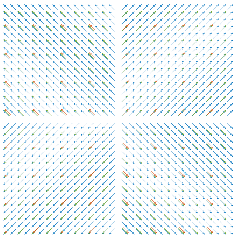
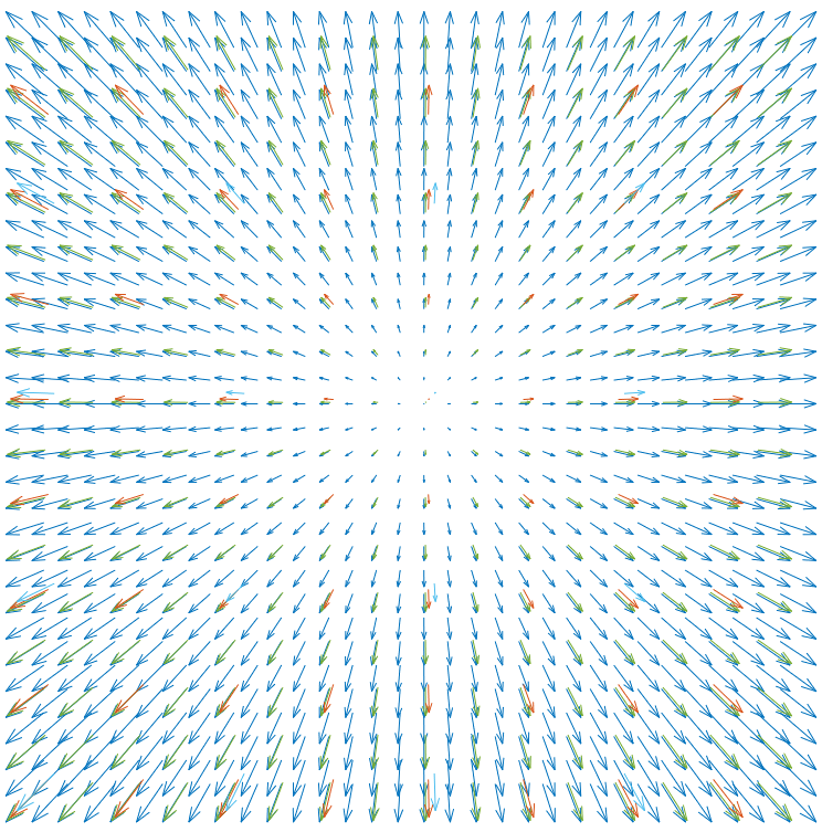
Figure 2: The level images and their gradient field for the two examples $f(x,y)=|x|+|y|$ (left) and of $f(x,y)=x^{2}+y^{2}$.

The situation changes in the case of non-smooth functions with sharp contours. While in the binary image in Fig. 3 the directions of the gradients are recognized correctly along the straight lines, their lengths are upscaled by a factor of $2^{n}$ which is due to the different resolution levels as the difference between two neighboring pixels is always either zero or one, but one divides by the resolution-dependent distance between the pixels at different levels to obtain the gradient. This can be compensated by rescaling the gradients by a factor of $2^{n}$ as shown on Fig. 3.

 

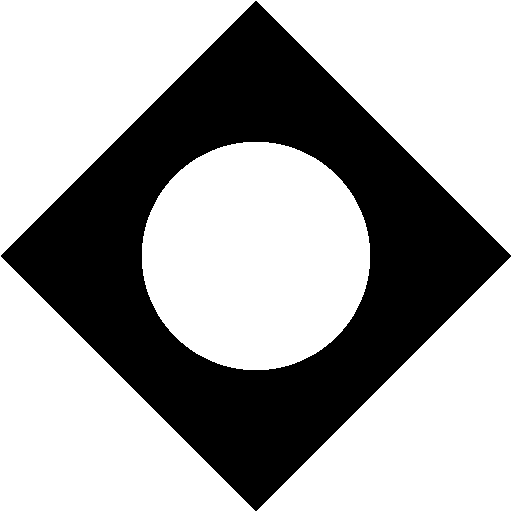
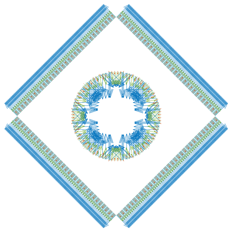
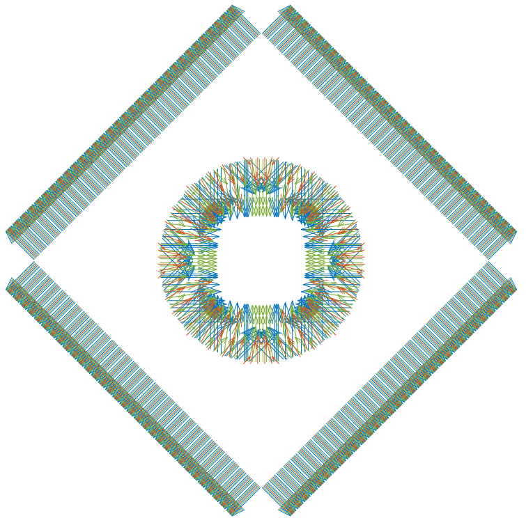
Figure 3: Simple synthetic image and the resulting gradient field, with the normalization factor $2^{n(1+s/2)+2}=2^{2n+2}$ (left) and with a normalization $2^{n+2}$ that compensates the resolution effects (right). In the image, different colors stand for different resolutions.

The estimate (10) is still a pointwise result, even if the error is bounded uniformly with respect to $\alpha$. We will explore this further in the next section to give an estimate of the TV norm of $f$ by means of wavelet coefficients, which also explains the normalization chosen in (11). So far, the estimates in (8) and (10) only work in the supremum norm.

4 Approximation of the TV norm

We will now derive estimates to show that the coefficient vectors $\hat{\boldsymbol{d}}_{\alpha}^{n}(f)$ formed from the wavelet coefficients with only one wavelet contribution give a good approximation for the TV norm of $f$ again directly from the wavelet coefficients.

To that end, let us recall that the TV norm of $f$, defined as

(12) $$\|f\|_{TV}:=\left\||\nabla f|_{2}\right\|_{1}=\int_{\mathbb{R}^{s}}\left|\nabla f(x)\right|_{2}\,dx,$$

where $|\cdot|_{2}$ denotes the Euclidean norm in $\mathbb{R}^{s}$. This functional plays a fundamental role in many imaging applications, at least since the work of Rudin, Osher and Fatemi [9], which made TV regularization a standard method in particular for image denoising. For a survey on TV based applications see also [1].

In the following we will need the Frobenius norm of the second derivative of $f\in C^{2}(\mathbb{R}^{s})$, i.e.,

$$\left|D^{2}f(x)\right|_{F}:=\left(\sum_{j,k=1}^{s}\left(\frac{\partial^{2}f(x)}{\partial x_{j}\partial x_{j}}\right)^{2}\right)^{1/2}.$$

We also define the functional

(13) $$H_{n}(f):=\sum_{\alpha\in\mathbb{Z}^{s}}2^{-ns}\max_{x\in x_{\alpha}^{n}+2^{-n}[-\frac{1}{2},\frac{1}{2}]}\left|D^{2}f(x)\right|_{F},\qquad n\in\mathbb{N},$$

which may take the value $\infty$, but has the property that $H_{n+1}(f)\leq H_{n}(f)$, $n\in\mathbb{N}_{0}$, and is clearly bounded from below. Functions for which $H_{n}(f)<\infty$, $n\in\mathbb{N}_{0}$, are for example compactly supported functions in $C^{2}(\mathbb{R}^{s})$ as then the Frobenius norm is bounded and the sum in (13) becomes a finite one.

We will prove in this section that the $\ell_{1}$ norm of the sequence $|\hat{\boldsymbol{d}}_{\alpha}^{n}|_{2}$, given as

$$\left\|\left|\hat{\boldsymbol{d}}^{n}\right|_{2}\right\|_{1}:=\sum_{\alpha\in\mathbb{Z}^{s}}\left|\hat{\boldsymbol{d}}_{\alpha}^{n}\right|_{2}=2^{n(1-s/2)+2}\sum_{\alpha\in\mathbb{Z}^{s}}\left(\sum_{j=1}^{s}\left(d_{\epsilon_{j},\alpha}^{n}\right)^{2}\right)^{1/2},$$

with $\hat{\boldsymbol{d}}^{n}:=\left(\hat{\boldsymbol{d}}_{\alpha}^{n}:\alpha\in\mathbb{Z}^{s}\right)$, is an approximation to $\|f\|_{TV}$, and we provide an explicit estimate for the error of this approximation. The result is as follows.

Theorem 4.1.

If $f\in C^{2}(\mathbb{R}^{s})$ and $H_{n}(f)<\infty$ for some $n\in\mathbb{N}_{0}$, then there exists, for any $n_{0}\in\mathbb{N}_{0}$, a constant $C>0$ that depends only on $n_{0}$ and $f$, such that

(14) $$\left|\left\|\left|\hat{\boldsymbol{d}}^{n}\right|_{2}\right\|_{1}-\|f\|_{TV}\right|\leq C2^{-n}\left\|\left|D^{2}f\right|_{F}\right\|_{1},\qquad n\geq n_{0}.$$

The slightly strange formulation of Theorem 4.1 will become clear from the proof. Indeed, the number $n_{0}$ can be used to control and reduce the constant $C$ by relying on high pass information only. More details on that in Remark 4.5 later.

Remark 4.2 (Normalization of coefficients).

1. The normalization of the coefficients $\hat{\boldsymbol{d}}_{\alpha}^{n}(f)$ in (11) may be somewhat surprising at first view because of its dependency on the dimensionality $s$. For $s=1$, coefficients at higher level are reweighted with an increasing weight $2^{n/2+2}$, for the image case $s=2$ the orthonormal normalization is just perfect, while for $s>2$ the weights decrease and penalize higher levels, which is particularly relevant for our main application, namely the volume case $s=3$.

2. Nevertheless, there is an explanation for this behavior. The TV norm considers the Euclidean length of the gradient, hence a one dimensional feature that scales like $2^{-n}$, while all other normalizations within the integrals are based on volumes that scale like $2^{-ns}$. This feature also appears when considering coefficients with respect to unnormalized wavelets.

3. It is important to keep in mind that it is the proper renormalization of the relevant coefficients and their treatment as vectors that allows us to approximate the TV norm by means of summing the coefficients.

4.1 Proof of the main theorem

We split the proof of Theorem 4.1 into two parts, first showing that $\left\|\left|\hat{\boldsymbol{d}}^{n}\right|_{2}\right\|_{1}$ is close to a cubature formula and then estimating the quality of the cubature formula. To that end, we define the sequence

$${\boldsymbol{f}}_{\nabla}^{n}:=\left(\nabla f(x_{\alpha}^{n}):\alpha\in\mathbb{Z}^{s}\right)$$

of sampled gradients of $f$.

Lemma 4.3.

If $f\in C^{2}(\mathbb{R}^{s})$ and $H_{n}(f)<\infty$ for some $n\in\mathbb{N}_{0}$, then there exists, for any $n_{0}\in\mathbb{N}_{0}$, a constant $C>0$ that depends only on $n_{0}$ and $f$ such that

(15) $$\left\|\left|\hat{\boldsymbol{d}}^{n}\right|_{2}-2^{-ns}\left|{\boldsymbol{f}}_{\nabla}^{n}\right|_{2}\right\|_{1}\leq 2^{-n}C\left\|\left|D^{2}f\right|_{F}\right\|_{1},\qquad n\geq n_{0}.$$

Proof 4.4.

We again use a Taylor formula at $x_{\alpha}^{n}$, this time with an integral remainder. It follows directly by applying the univariate formula to $t\mapsto f\left(x_{\alpha}+t(x-x_{\alpha}^{n})\right)$, $t\in[0,1]$, and takes the form

(16) $$f(x)=f(x_{\alpha}^{n})+\nabla f(x_{\alpha}^{n})^{T}(x-x_{\alpha}^{n})+\int_{0}^{1}(1-\xi)(x-x_{\alpha}^{n})^{T}D^{2}f\left(x_{\alpha}^{n}+\xi(x-x_{\alpha}^{n})\right)(x-x_{\alpha}^{n})\,d\xi.$$

Using again Lemma 3.1, it follows for $j=1,\dots,s$ that

(17) $$d_{\epsilon_{j},\alpha}^{n}(f)=\int_{\mathbb{R}^{s}}f(x)\psi_{\epsilon_{j},\alpha}^{n}(x)\,dx=-2^{-n(1+s/2)-2}\frac{\partial f}{\partial x_{j}}(x_{\alpha}^{n})+h_{j,\alpha}^{n}$$

where

$$h_{j,\alpha}^{n}:=\int_{\mathbb{R}^{s}}\int_{0}^{1}(1-\xi)(x-x_{\alpha}^{n})^{T}D^{2}f\left(x_{\alpha}^{n}+\xi(x-x_{\alpha}^{n})\right)(x-x_{\alpha}^{n})\,\psi_{\epsilon_{j},\alpha}^{n}(x)\,d\xi dx$$

can be estimated as

$$\left|h_{j,\alpha}^{n}\right|$$

$$\leq 2^{ns/2}\int_{0}^{1}(1-\xi)\int_{x_{\alpha}^{n}+2^{-n}[-\frac{1}{2},\frac{1}{2}]}\left|(x-x_{\alpha}^{n})^{T}D^{2}f\left(x_{\alpha}^{n}+\xi(x-x_{\alpha}^{n})\right)(x-x_{\alpha}^{n})\right|\,dx\,d\xi$$

$$\leq 2^{ns/2}\int_{0}^{1}(1-\xi)\int_{2^{-n}[-\frac{1}{2},\frac{1}{2}]}\left|x\right|_{2}^{2}\left|D^{2}f\left(x_{\alpha}^{n}+\xi x\right)\right|_{F}\,dx\,d\xi$$

$$\leq s2^{-2n-2+ns/2}\int_{0}^{1}(1-\xi)\int_{2^{-n}[-\frac{1}{2},\frac{1}{2}]}\left|D^{2}f\left(x_{\alpha}^{n}+\xi x\right)\right|_{F}\,dx\,d\xi.$$

The last expression is independent of $j$, hence, if we define ${\boldsymbol{h}}_{\alpha}^{n}=\left(h_{j,\alpha}^{n}:j=1,\dots,s\right)$, we get that

(18) $$\left|{\boldsymbol{h}}_{\alpha}^{n}\right|_{2}\leq s^{3/2}2^{-2n-2+ns/2}\int_{0}^{1}(1-\xi)\int_{2^{-n}[-\frac{1}{2},\frac{1}{2}]}\left|D^{2}f\left(x_{\alpha}^{n}+\xi x\right)\right|_{F}\,dx\,d\xi$$

The step functions

$$g_{+}^{n}:=\sum_{\alpha\in\mathbb{Z}^{s}}2^{-ns}\left(\max_{x\in x_{\alpha}^{n}+2^{-n}[-\frac{1}{2},\frac{1}{2}]}\left|D^{2}f(x)\right|\right)\,\chi_{[0,1]^{s}}(2^{n}\cdot-\alpha),\qquad n\in\mathbb{N}_{0}$$

converge monotonically decreasing and pointwise towards $\left|D^{2}f(x)\right|$ and satisfy $0\leq\|g_{+}^{n}\|_{1}=H_{n}(f)$ which is finite for sufficiently large $n$. Hence, by the Beppo Levi Theorem, $\left|D^{2}f(x)\right|\in L_{1}(\mathbb{R}^{s})$. In addition,

$$g_{-}^{n}:=\sum_{\alpha\in\mathbb{Z}^{s}}2^{-ns}\left(\min_{x\in x_{\alpha}^{n}+2^{-n}[-\frac{1}{2},\frac{1}{2}]}\left|D^{2}f(x)\right|\right)\,\chi_{[0,1]^{s}}(2^{n}\cdot-\alpha)$$

is trivially bounded from below by $0$, from above by $\left|D^{2}f(x)\right|$ and converges monotonically increasing towards $\left|D^{2}f(x)\right|$. Since for any $\xi\in[0,1]$ we have that

$$\min_{x\in x_{\alpha}^{n}+2^{-n}[-\frac{1}{2},\frac{1}{2}]}\left|D^{2}f(x)\right| \leq 2^{ns}\int_{2^{-n}[-\frac{1}{2},\frac{1}{2}]}\left|D^{2}f\left(x_{\alpha}^{n}+\xi x\right)\right|_{F}\,dx$$

$$\leq \max_{x\in x_{\alpha}^{n}+2^{-n}[-\frac{1}{2},\frac{1}{2}]}\left|D^{2}f(x)\right|_{F},$$

and since $\|g_{\pm}\|_{1}\to\left\|\left|D^{2}f(x)\right|_{F}\right\|_{1}$ it follows that

$$\lim_{n\to\infty}\sum_{\alpha\in\mathbb{Z}^{s}}\int_{2^{-n}[-\frac{1}{2},\frac{1}{2}]}\left|D^{2}f\left(x_{\alpha}^{n}+\xi x\right)\right|_{F}\,dx=\int_{\mathbb{R}^{s}}\left|D^{2}f(x)\right|_{F}\,dx$$

uniformly in $\xi$. In particular, there exists, for any $n_{0}\in\mathbb{N}_{0}$, a constant $C=C(n_{0},f)$ such that

$$\sum_{\alpha\in\mathbb{Z}^{s}}\int_{2^{-n}[-\frac{1}{2},\frac{1}{2}]}\left|D^{2}f\left(x_{\alpha}^{n}+\xi x\right)\right|_{F}\,dx\leq C\int_{\mathbb{R}^{s}}\left|D^{2}f(x)\right|_{F}\,dx,\qquad n\geq n_{0},$$

and

(19) $$\lim_{n_{0}\to\infty}C(n_{0},f)=1.$$

Under the assumption that $n\geq n_{0}$ this yields that

(20) $$\sum_{\alpha\in\mathbb{Z}^{s}}\left|{\boldsymbol{h}}_{\alpha}^{n}\right|_{2}\leq\frac{C}{2}s^{3/2}2^{-2n-2+ns/2}\left\|\left|D^{2}f\right|_{F}\right\|_{1}.$$

Multiplying (17) by $-2^{n(1-s/2)+2}$ we get that

$$\left|-2^{n(1-s/2)+2}d_{\epsilon_{j},\alpha}^{n}(f)-2^{-ns}\frac{\partial f}{\partial x_{j}}(x_{\alpha}^{n})\right|\leq 2^{n(1-s/2)+2}\left|h_{j,\alpha}\right|,$$

hence,

$$\left|\left|\hat{\boldsymbol{d}}_{\alpha}^{n}\right|_{2}-2^{-ns}\left|\nabla f(x_{\alpha}^{n})\right|_{2}\right|\leq\left|\hat{\boldsymbol{d}}_{\alpha}^{n}-2^{-ns}\nabla f(x_{\alpha}^{n})\right|_{2}\leq 2^{n(1-s/2)+2}\left|{\boldsymbol{h}}_{\alpha}^{n}\right|_{2}.$$

Summing this over $\alpha\in\mathbb{Z}^{s}$ and substituting (20) we then obtain

(21) $$\sum_{\alpha\in\mathbb{Z}^{s}}\left|\left|\hat{\boldsymbol{d}}_{\alpha}^{n}\right|_{2}-2^{-ns}\left|\nabla f(x_{\alpha}^{n})\right|_{2}\right|\leq 2^{-n}C\frac{s^{3/2}}{2}\left\|\left|D^{2}f\right|_{F}\right\|_{1},$$

which is (15).

Remark 4.5.

The constant $C$ in (15) can be chosen as $\frac{s^{3/2}}{2}+\varepsilon$ for any $\varepsilon>0$ by making $n_{0}$ sufficiently large. In practice this means to avoid relatively low pass content of the wavelet transformation which approximates the gradient only in a rather poor way. Of course, the dependency of the constant $C$ on $f$ would also have to be taken into account.

We remark that (15) immediately implies

(22) $$\left|\left\|\left|\hat{\boldsymbol{d}}^{n}\right|_{2}\right\|_{1}-\sum_{\alpha\in\mathbb{Z}^{s}}2^{-ns}\left|\nabla f(x_{\alpha}^{n})\right|_{2}\right|\leq C2^{-n}\left\|\left|D^{2}f\right|_{F}\right\|_{1},\qquad n\geq n_{0},$$

which shows that $\left\|\left|\hat{\boldsymbol{d}}^{n}\right|_{2}\right\|_{1}$ approximates the cubature formula for the TV norm. Now we only have to recall the approximation quality of the cubature formula. This follows by standard arguments which we include for completeness.

Lemma 4.6.

If $f\in C^{2}(\mathbb{R}^{s})$ and $H_{n}(f)<\infty$ for some $n\in\mathbb{N}_{0}$, then there exists, for any $n_{0}\in\mathbb{N}_{0}$, a constant $C>0$ that depends only on $n_{0}$ and $f$ such that

(23) $$\left|\left\|2^{-ns}\left|{\boldsymbol{f}}_{\nabla}^{n}\right|_{2}\right\|_{1}-\|f\|_{TV}\right|\leq C2^{-n}\left\|\left|D^{2}f\right|_{F}\right\|_{1},\qquad n\geq n_{0}.$$

Proof 4.7.

Again we employ a Taylor expansion, this time using

$$\nabla f(x)=\nabla f(x_{\alpha}^{n})+\int_{0}^{1}D^{2}f\left(x_{\alpha}^{n}+\xi(x-x_{\alpha}^{n})\right)(x-x_{n}^{\alpha})\,d\xi$$

to get by similar transformations as in the proof of Lemma 4.3

$$\int_{x_{\alpha}+2^{-n}[-\frac{1}{2},\frac{1}{2}]}\left|\nabla f(x)-\nabla f(x_{\alpha}^{n})\right|_{2}\,dx\leq\int_{2^{-n}[-\frac{1}{2},\frac{1}{2}]}\int_{0}^{1}\left|D^{2}f\left(x_{\alpha}^{n}+\xi x\right)\right|_{F}|x|_{2}\,d\xi,$$

hence

$$\left|2^{-ns}\left|\nabla f(x_{\alpha}^{n})\right|_{2}-\int_{x_{\alpha}+2^{-n}[-\frac{1}{2},\frac{1}{2}]}\left|\nabla f(x)\right|_{2}\right|$$

$$\leq \sqrt{s}2^{-n-1}\int_{2^{-n}[-\frac{1}{2},\frac{1}{2}]}\int_{0}^{1}\left|D^{2}f\left(x_{\alpha}^{n}+\xi x\right)\right|_{F}\,d\xi.$$

By the same arguments as in Lemma 4.3, there exist $n_{0}$ and $C>0$ such that

$$\left|\sum_{\alpha\in\mathbb{Z}^{s}}2^{-ns}\left|\nabla f(x_{\alpha}^{n})\right|_{2}-\int_{\mathbb{R}^{s}}\left|\nabla f(x)\right|_{2}\,dx\right|\leq\frac{\sqrt{s}}{2}2^{-n}C\left\|\left|D^{2}f\right|_{F}\right\|_{1},$$

giving (23).

Now it is easy to complete the proof of the main theorem.

Proof 4.8 (Proof of Theorem 4.1).

Combining (22) and (23), the triangle inequality gives

$$\left|\left\||\hat{\boldsymbol{d}}^{n}|_{2}\right\|_{1}-\|f\|_{TV}\right|\leq C2^{-n}\left\|\left|D^{2}f\right|_{F}\right\|_{1},\qquad n\geq n_{0},$$

where the constant can be anything of the form

$$\frac{s^{3/2}}{2}+\frac{s^{1/2}}{2}+\varepsilon=\sqrt{s}\frac{s+1}{2}+\varepsilon,\qquad\varepsilon>0,$$

by once more selecting a sufficiently high value for $n_{0}$.

4.2 Estimation over several levels

The estimate in (14) holds for any sufficiently high wavelet level separately and the error of the estimate decreases with $n$, so it might appear reasonable to approximate the TV norm just by the maximal level. Indeed, in practical applications one starts with finite data on a certain finest level $n_{1}+1$, i.e.,

$$c_{\alpha}^{n_{1}+1}(f):=\int_{\mathbb{R}^{s}}f(x)\,\psi_{0,\alpha}^{n_{1}+1}(x)\,dx,\qquad\alpha\in\mathbb{Z}^{s},$$

and then computes the coefficients in the wavelet decomposition

$$\sum_{\alpha\in\mathbb{Z}^{s}}c_{\alpha}^{n_{1}+1}(f)\,\psi_{0,\alpha}^{n_{1}+1}=\sum_{k=0}^{n_{1}}\sum_{\theta\in\{0,1\}^{s}\setminus\{0\}}\sum_{\alpha\in\mathbb{Z}^{s}}d_{\theta,\alpha}^{k}(f)\,\psi_{\theta,\alpha}^{k}.$$

To get an approximation of the TV norm that uses at the same time as many levels as possible, namely $\hat{\boldsymbol{d}}^{n}$, $n=n_{0},\dots,n_{1}$, we make use of suitable averaging to obtain almost the same rate of accuracy as by the highest level alone.

Proposition 4.9.

If under the assumptions of Theorem 4.1 we define

(25) $$\hat{\boldsymbol{d}}:=\sum_{n=n_{0}}^{n_{1}}\mu_{n}\,\hat{\boldsymbol{d}}^{n},\qquad\mu_{n}:=\frac{2^{n-n_{1}}}{2-2^{n_{0}-n_{1}}},\quad n=n_{0},\dots,n_{1},$$

then

(26) $$\left|\left\||\hat{\boldsymbol{d}}|_{2}\right\|_{1}-\|f\|_{TV}\right|\leq C(n_{1}-n_{0})2^{-n_{1}}\left\|\left|D^{2}f\right|_{F}\right\|_{1}.$$

Proof 4.10.

By construction, $\sum\mu_{n}=1$, and we thus have that

$$\left|\left\||\hat{\boldsymbol{d}}|_{2}\right\|_{1}-\|f\|_{TV}\right|$$

$$= \left|\left\|\sum_{n=n_{0}}^{n_{1}}\mu_{n}\left|\hat{\boldsymbol{d}}^{n}\right|_{2}\right\|_{1}-\sum_{n=n_{0}}^{n_{1}}\mu_{n}\|f\|_{TV}\right|\leq\sum_{n=n_{0}}^{n_{1}}\mu_{n}\left|\left\||\hat{\boldsymbol{d}}|_{2}\right\|_{1}-\|f\|_{TV}\right|$$

$$\leq \frac{C}{2-2^{n_{0}-n_{1}}}\left\|\left|D^{2}f\right|_{F}\right\|_{1}\sum_{k=n_{0}}^{n_{1}}2^{n-n_{1}}2^{-k}\leq(n_{1}-n_{0})C2^{-n_{1}}\left\|\left|D^{2}f\right|_{F}\right\|_{1},$$

which is (26).

Of course, any averaging of $\left\|\left|\hat{\boldsymbol{d}}^{n}\right|_{2}\right\|_{1}$ would yield an approximation for the TV norm, but the particular choice of the weights in (25) ensures that the rate of convergence obtained by this averaging process is the same as that on the highest level, only affected by the “logarithmic” number $n_{1}-n_{0}$ of the levels incorporated in the approximation process.

5 Approximate TV regularization

TV regularization is a standard procedure for many imaging applications nowadays, especially for denoising. It consists of solving, for a given image $f$, an optimization problem

(27) $$\min_{u}\frac{1}{2}\left\|f-u\right\|_{2}^{2}+\lambda\|u\|_{TV},\qquad\lambda>0,$$

where the regularization term $\lambda\|u\|_{TV}$ enforces a smooth or less noisy behavior of $u$ whose influence is controlled by the parameter $\lambda$. In most applications, $\|u\|_{TV}$ is computed for discrete data $u$ by numerical differentiation, usually by means of differences. In particular, this not only requires access to the full image, the discrete gradient needs an additional amount of $s$ times the memory consumption of the original image. Since this is mostly unacceptable in our application where the image is orders of magnitude larger than the available memory, the straightforward approach is to use the wavelet coefficients as a computationally efficient approximation for $\|u\|_{TV}$.

A relaxation of the optimization problem (27) can be solved explicitly by standard methods that we are going to explain now. To that end, we assume that $f$ and $u$ are given as finite orthonormal wavelet expansions

$$f = \sum_{\alpha\in\mathbb{Z}^{s}}c_{\alpha}(f)\,\psi_{0,\alpha}+\sum_{n=0}^{n_{1}}\sum_{\theta\in\{0,1\}^{s}\setminus\{0\}}\sum_{\alpha\in\mathbb{Z}^{s}}d_{\theta,\alpha}^{n}(f)\,\psi_{\theta,\alpha}^{n},$$

$$u = \sum_{\alpha\in\mathbb{Z}^{s}}c_{\alpha}(u)\,\psi_{0,\alpha}+\sum_{n=0}^{n_{1}}\sum_{\theta\in\{0,1\}^{s}\setminus\{0\}}\sum_{\alpha\in\mathbb{Z}^{s}}d_{\theta,\alpha}^{n}(u)\,\psi_{\theta,\alpha}^{n}.$$

Since orthonormality implies that

$$\|f-u\|_{2}^{2}=\sum_{\alpha\in\mathbb{Z}^{s}}\left(c_{\alpha}(f)-c_{\alpha}(u)\right)^{2}+\sum_{n=0}^{n_{1}}\sum_{\theta\in\{0,1\}^{s}\setminus\{0\}}\sum_{\alpha\in\mathbb{Z}^{s}}\left(d_{\theta,\alpha}^{n}(f)-d_{\theta,\alpha}^{n}(u)\right)^{2},$$

the first term in (27) can be differentiated with respect to the wavelet coefficients yielding

$$\frac{\partial}{\partial c_{\alpha}(u)}\frac{1}{2}\|f-u\|_{2}^{2} = c_{\alpha}(f)-c_{\alpha}(u),$$

$$\frac{\partial}{\partial d_{\alpha,\theta}^{n}(u)}\frac{1}{2}\|f-u\|_{2}^{2} = d_{\alpha,\theta}^{n}(f)-d_{\alpha,\theta}^{n}(u).$$

For the $L_{1}$ term we use the approximation $\|u\|_{TV}\approx\left\|\left|\hat{\boldsymbol{d}}(u)\right|_{2}\right\|_{1}$ of Proposition 4.9, i.e., we solve the approximate problem

(28) $$\min_{u}\frac{1}{2}\|f-u\|_{2}^{2}+\lambda\left\|\left|\hat{\boldsymbol{d}}(u)\right|_{2}\right\|_{1}$$

with the regularity term

$$F(u):=\sum_{\alpha\in\mathbb{Z}^{s}}\left|\hat{\boldsymbol{d}}_{\alpha}(u)\right|_{2}=\sum_{n=n_{0}}^{n_{1}}\mu_{n}\left|\hat{\boldsymbol{d}}_{\alpha}^{n}(u)\right|_{2},$$

whose (generally set-valued) subgradient is composed of

$$\partial_{\hat{\boldsymbol{d}}_{\alpha}^{n}(u)}F(u)=\mu_{n}\begin{cases}B_{1}(0),&\hat{\boldsymbol{d}}_{\alpha}^{n}=0,\\ \dfrac{\hat{\boldsymbol{d}}_{\alpha}^{n}}{\left|\hat{\boldsymbol{d}}_{\alpha}^{n}\right|_{2}},&\hat{\boldsymbol{d}}_{\alpha}^{n}\neq 0,\\ \end{cases}\qquad\alpha\in\mathbb{Z}^{s},\quad n=n_{0},\dots,n_{1},$$

where $B_{1}(0)=\{x\in\mathbb{R}^{s}:|x|_{2}=1\}$. A necessary and sufficient condition for $u$ to be a solution of the convex optimization problem (28) is that

$$0\in\partial\left(\frac{1}{2}\|f-u\|_{2}^{2}+\lambda\left\|\left|\hat{\boldsymbol{d}}(u)\right|_{2}\right\|_{1}\right),$$

cf. [8], which is in turn equivalent to

(29) $$\begin{array}[]{rclrl}c_{\alpha}(u)&=&c_{\alpha}(f),&&\alpha\in\mathbb{Z}^{2},\\ d_{\theta,\alpha}^{n}(u)&=&d_{\theta,\alpha}^{n}(f),&&\alpha\in\mathbb{Z}^{s},\,|\theta|>1,\,n=n_{0},\dots,n_{1},\end{array}$$

and, taking into account the renormalization (11) of the coefficients in the orthogonal expansion,

(30) $$0\in-2^{-n(1-s/2)-2}\left(\hat{\boldsymbol{d}}_{\alpha}^{n}(f)-\hat{\boldsymbol{d}}_{\alpha}^{n}(u)\right)+\lambda\partial_{\hat{\boldsymbol{d}}_{\alpha}^{n}(u)}F(u),\qquad\alpha\in\mathbb{Z}^{s},\,n=n_{0},\dots,n_{1},$$

that is, for $\alpha\in\mathbb{Z}^{s}$, $n=n_{0},\dots,n_{1}$,

(31) $$\hat{\boldsymbol{d}}_{\alpha}^{n}(f) \in \hat{\boldsymbol{d}}_{\alpha}^{n}(u)+2^{n(1-s/2)+2}\,\lambda\partial_{\hat{\boldsymbol{d}}_{\alpha}^{n}(u)}F(u)$$

$$= \begin{cases}2^{n(1-s/2)+2}\mu_{n}\lambda B_{1}(0),&\hat{\boldsymbol{d}}_{\alpha}^{n}(u)=0,\\ \left(1+\lambda\dfrac{2^{n(1-s/2)+2}\mu_{n}}{\left|\hat{\boldsymbol{d}}_{\alpha}^{n}(u)\right|_{2}}\right)\hat{\boldsymbol{d}}_{\alpha}^{n}(u),&\hat{\boldsymbol{d}}_{\alpha}^{n}(u)\neq 0.\end{cases}$$

From this observation we get the explicit representation of the solution of (28). We add the well-known short proof for completeness and the reader’s convenience.

Proposition 5.1.

The solution of (30) can be computed by soft thresholding the length of the coefficient vectors ${\boldsymbol{d}}_{\alpha}^{n}(f)$, i.e., as

(32) $${\boldsymbol{d}}_{\alpha}^{n}(u)=\left(1-\frac{\mu_{n}\lambda}{\left|{\boldsymbol{d}}_{\alpha}^{n}(f)\right|_{2}}\right)_{+}{\boldsymbol{d}}_{\alpha}^{n}(f),\qquad\alpha\in\mathbb{Z}^{s},\,n=n_{0},\dots,n_{1}.$$

Proof 5.2.

The first case in (31) means that $\hat{\boldsymbol{d}}_{\alpha}^{n}(u)=0$ which is equivalent to $\left|\hat{\boldsymbol{d}}_{\alpha}^{n}(f)\right|_{2}\leq\lambda_{n}:=2^{n(1-s/2)+2}\mu_{n}$, while otherwise (32) implies that $\left|\hat{\boldsymbol{d}}_{\alpha}^{n}(u)\right|_{2}=\left|\hat{\boldsymbol{d}}_{\alpha}^{n}(f)\right|_{2}-\lambda_{n}$ and therefore

$$\left(1+\frac{\lambda_{n}}{\left|\hat{\boldsymbol{d}}_{\alpha}^{n}(u)\right|_{2}}\right)\hat{\boldsymbol{d}}_{\alpha}^{n}(u)=\left(1+\frac{\lambda_{n}}{\left|\hat{\boldsymbol{d}}_{\alpha}^{n}(f)\right|_{2}-\lambda_{n}}\right)\left(1-\frac{\lambda_{n}}{\left|\hat{\boldsymbol{d}}_{\alpha}^{n}(f)\right|_{2}}\right)\hat{\boldsymbol{d}}_{\alpha}^{n}(f)=\hat{\boldsymbol{d}}_{\alpha}^{n}(f),$$

which yields that

$$\hat{\boldsymbol{d}}_{\alpha}^{n}(u)=\left(1-\dfrac{\lambda_{n}}{\left|\hat{\boldsymbol{d}}_{\alpha}^{n}(f)\right|_{2}}\right)\hat{\boldsymbol{d}}_{\alpha}^{n}(f)=\left(1-\lambda\dfrac{2^{n(1-s/2)+2}\mu_{n}}{\left|\hat{\boldsymbol{d}}_{\alpha}^{n}(f)\right|_{2}}\right)\hat{\boldsymbol{d}}_{\alpha}^{n}(f).$$

Substituting (11) then immediately gives (32).

One might also approximate the TV norm in (27) by a single level set of wavelet coefficients and solve

$$\min_{u}\frac{1}{2}\|f-u\|_{2}+\lambda\left\|\left|\hat{\boldsymbol{d}}^{n}(u)\right|_{2}\right\|_{1}$$

for some $n$, which is solved by the soft thresholding

(33) $${\boldsymbol{d}}_{\alpha}^{n}(u)=\left(1-\frac{\lambda}{\left|{\boldsymbol{d}}_{\alpha}^{n}(f)\right|_{2}}\right)_{+}{\boldsymbol{d}}_{\alpha}^{n}(f),\qquad\alpha\in\mathbb{Z}^{s},$$

and even apply this shrinkage to the range $n=n_{0},\dots,n_{1}$. This corresponds to solving the optimization problems

$$\min_{u}\left\|f_{n}-u_{n}\right\|_{2}^{2}+\lambda\left\|\left|\hat{\boldsymbol{d}}^{n}(u)\right|_{2}\right\|_{1},\qquad n=n_{0},\dots,n_{1},$$

where

$$f_{n}=\sum_{\alpha\in\mathbb{Z}^{s}}c_{\alpha}(f)\,\psi_{0,\alpha}+\sum_{k=0}^{n}\sum_{\theta\in\{0,1\}^{s}\setminus\{0\}}\sum_{\alpha\in\mathbb{Z}^{s}}d_{\theta,\alpha}^{k}(f)\,\psi_{\theta,\alpha}^{k}$$

denotes the projection of $f$ on the first $n$ levels of the multiresolution with an analogous definition of $u_{n}$. This results in a differently weighted shrinkage process, however with a larger error between the $\left\|\left|\hat{\boldsymbol{d}}^{n}(u)\right|_{2}\right\|_{1}$ and $\|u\|_{TV}$.

To conclude, we again make a short comparison with [11, 13] where wavelet shrinkage is related to diffusion filtering processes. Nevertheless, our findings show that for an approximation of the TV functional the shrinkage process has to be adapted:

1. The shrinkage has to be applied to the length of the vectors ${\boldsymbol{d}}_{\alpha}^{n}(f)$ and not to its components separately. Also only those coefficients have to be take into account that contain a single wavelet component.

2. The coefficients have to be properly renormalized and this renormalization depends on the level of the wavelet coefficients.

3. It matters that we use Haar wavelets here. The reconstruction of first derivatives requires, at least in our approach, univariate wavelets with only a single vanishing moment, the simple expressions for proper renormalization are even due to the explicit nature and support size of the wavelets.

Under these conditions, we can give precise error estimates for the procedure that works entirely on the wavelet coefficients.

6 Applications to computed tomography

Discrete data is usually modeled as a real-valued function on $\mathbb{Z}^{s}$ with compact support. For the application to discrete CT data in $s=3$ this means to consider functions $g:\mathbb{R}^{3}\rightarrow\mathbb{R}$ that are constant on intervals $[0,1)+\alpha$, $\alpha\in\mathbb{Z}^{3}$, representing the reconstructed voxels, and which are zero outside of $\left[0,2^{m}\right)^{3}$ for some $m\in\mathbb{N}_{0}$. In practice, we set $m$ to the minimal number such that the support of a dataset is completely contained within this interval. To account for this situation, we set up an alternative one-dimensional wavelet basis originating from the tensorized, iterated application of the orthogonal transform matrix

$$H:=2^{-1/2}\left(\begin{array}[]{cc}1&1\\ 1&-1\end{array}\right)$$

to discrete data. For example, the one-dimensional array $(1,2)$ is interpreted as a function $f=1\chi_{[0,1)}+2\chi_{[1,2)}$ with wavelet coefficients $c(f)=2^{-1/2}\cdot 3$ and $d(f)=-2^{-1/2}$. However, we want the average coefficient $c(f)$ to live on the interval $[0,1]$ as above, i.e., we need proper rescaling. We point out this straightforward but important scaling process for the sake of completeness next.

6.1 Haar wavelet coefficient scaling

The above way of the discrete transform is connected to the wavelet basis built on (1) via the $L_{2}(\mathbb{R}^{s})$ isometry

$$T_{s,m}:\left(\mathbb{R}^{s}\rightarrow\mathbb{R}\right)\rightarrow\left(\mathbb{R}^{s}\rightarrow\mathbb{R}\right),\qquad f\mapsto 2^{-ms/2}f\left(2^{-m}\cdot\right),$$

yielding the scaling and wavelet functions

$$\tilde{\psi}_{0,m}:=T_{1,m}\psi_{0},\quad\tilde{\psi}_{1,m}:=T_{1,m}\psi_{1}$$

and, analogously,

$$\tilde{\psi}^{n}_{1,k,m}:=T_{1,m}\psi^{n}_{1,k},\qquad k\in\mathbb{Z},n\in\mathbb{N}_{0},$$

completing another orthonormal basis of $L_{2}(\mathbb{R})$ such that

$$\tilde{\psi}^{n}_{1,k,m}=2^{n/2}\tilde{\psi}_{1,m}\left(2^{n}\cdot-2^{m}k\right),\qquad k\in\mathbb{Z},n\in\mathbb{N}_{0}.$$

Then, for $f,g\in L_{2}(\mathbb{R})$ such that $g=T_{1,m}f$, we get for $k\in\mathbb{Z}$,

$$\tilde{c}_{k,m}(g):=\int_{\mathbb{R}}g(t)\tilde{\psi}_{0,m}\left(t-2^{m}k\right)dt=\int_{\mathbb{R}}f(t)\psi_{0}(t-k)dt=c_{k}(f),$$

and

$$\tilde{d}^{n}_{k,m}(g):=\int_{\mathbb{R}}g(t)\tilde{\psi}^{n}_{1,k,m}(t)dt=\int_{\mathbb{R}}f(t)\psi^{n}_{1,k}(t)dt=d^{n}_{k,m}(f),\qquad k\in\mathbb{Z},n\in\mathbb{N}_{0},$$

allowing us to eventually build a bridge to the previous sections by considering $f=T_{1,m}^{-1}g$ when discrete data $g$ is given. In $s$ dimensions, we define

$$\tilde{\psi}_{\theta,m}(x):=\prod_{j=1}^{s}\tilde{\psi}_{\theta_{j},m}(x_{j})=2^{-ms/2}\psi_{\theta}\left(2^{-m}x\right)=T_{s,m}\psi_{\theta}(x)$$

for $\theta\in\{0,1\}^{s}\setminus\{0\}$ as in (3) and use $\tilde{\psi}_{0,m}=T_{s,m}\psi_{0}=2^{-ms/2}\chi_{\left[0,2^{m}\right]^{s}}$. Given $g$, we consider $f=T_{s,m}^{-1}(g)$ and calculate

$$\tilde{c}_{\alpha}(g):=\int_{\mathbb{R}^{s}}g(t)\tilde{\psi}_{0,m}\left(t-2^{m}\alpha\right)dt=\int_{\mathbb{R}^{2}}f(t)\psi_{0}(t-\alpha)dt=c_{\alpha}(f)$$

for $\alpha\in\mathbb{Z}^{s}$. Similarly, $\tilde{d}^{n}_{\theta,\alpha,m}(g)=d^{n}_{\theta,\alpha}(f)$ since

$$\tilde{d}^{n}_{\theta,\alpha,m}(g)=2^{(n-m)s/2}\int_{\mathbb{R}^{s}}g(t)\phi_{\theta}\left(2^{n-m}t-\alpha\right)dt=2^{ns/2}\int_{\mathbb{R}^{s}}f(t)\phi_{\theta}\left(2^{n}-\alpha\right)dt$$

for $\alpha\in\mathbb{Z}^{s}$, $n\in\mathbb{N}_{0}$. Thus, we can reuse the coefficients from the discrete transform of $g$ without modifications in our TV regularization approach with the corresponding, properly scaled function $f=2^{ms/2}g\left(2^{m}\cdot\right)$. Regarding the minimization problem (28), using

$$\hat{\boldsymbol{d}}^{n}_{\alpha,m}(\tilde{u}):=-2^{n(1-s/2)+2}\tilde{{\boldsymbol{d}}}^{n}_{\alpha,m},\qquad\tilde{{\boldsymbol{d}}}^{n}_{\alpha,m}(\tilde{u}):=\begin{pmatrix}\tilde{d}_{\epsilon_{j},\alpha,m}(\tilde{u}):j=1,\ldots,s\end{pmatrix}\in\mathbb{R}^{s},$$

for $\alpha\in\mathbb{Z}^{s}$, $n\in\mathbb{N}_{0}$, analogously to (11) and due to $\tilde{d}^{n}_{\epsilon_{j},\alpha,m}(\tilde{u})=d^{n}_{\epsilon_{j},\alpha}\left(T_{s,m}^{-1}\left(\tilde{u}\right)\right)$, $j=1,\ldots,s$, $\alpha\in\mathbb{Z}^{s}$, $n\in\mathbb{N}_{0}$, we note that

$$\min_{u}\frac{1}{2}\|f-u\|_{2}^{2}+\lambda\left\|\left|\hat{\boldsymbol{d}}(u)\right|_{2}\right\|_{1}=\min_{\tilde{u}}\frac{1}{2}\|g-\tilde{u}\|_{2}^{2}+\lambda\left\|\left|\hat{\boldsymbol{d}}_{m}(\tilde{u})\right|_{2}\right\|_{1}$$

after substituting $\tilde{u}:=T_{s,m}u$. This finally verifies that the $L_{2}(\mathbb{R}^{s})$-isometric scaling allows us to use the discrete Haar wavelet coefficients directly.

6.2 Example dataset

 

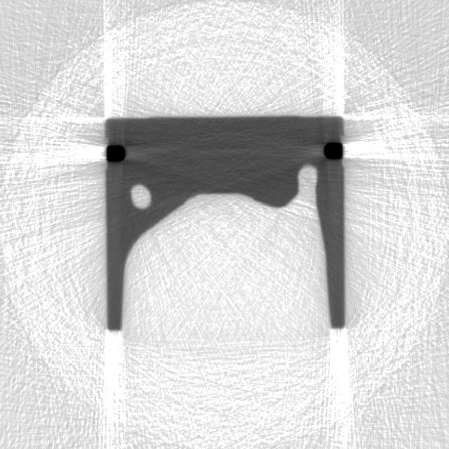
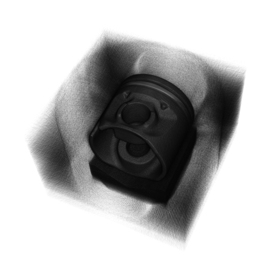
Figure 4: Slice and three-dimensional view of the motor piston with additional gamma correction and logarithmic scaling for emphasizing the presence of noise.

To illustrate the results, we will use a typical industrial data set, a Mahle motor piston, as a running example. In Fig. 4, we see a slice view alongside a three-dimensional view, where the different materials are visible: surrounding (noisy) air, foam (piston fixation), aluminum (piston body) and iron (ring). The dataset itself is of the small size $464\times 464\times 414$ and contains nonnegative integer values. Due to its well separated materials and the fact that we can also compute its TV norm explicitly by means of discrete differences for comparison, it is nevertheless useful for illustration.

6.3 Practical issues

We apply our thresholding method, called LiveTV, to the piston data set; the name is due to the fact that the regularization can be done in real time during the multi-resolution visualization. In addition, we use a modification, called SparseTV, where all coefficients are set to zero if the wavelet gradient is thresholded to zero at a certain location. The rationale behind this is, on the one hand, the assumption of locally homogeneous data, and, secondly, the observation stated in Remark 3.6, that in such a situation, the wavelet coefficients with $|\theta|\geq 2$ should decay faster than those with $|\theta|=1$. The justifies the heuristic to set them to zero if the gradient is below the threshold level.

6.4 Results

Threshold $\lambda$	$10^{1}$	$10^{2}$	$10^{3}$	$10^{4}$	$10^{5}$
Relative Discrete TV Norm	$99.7\%$	$97\%$	$81\%$	$73\%$	$76\%$
Relative Approx. Wavelet TV Norm	$99\%$	$93\%$	$49\%$	$20\%$	$8.5\%$
Relative $L_{2}$ Error	$0.041\%$	$0.38\%$	$2.9\%$	$6.5\%$	$13\%$
Peak Signal-to-Noise Ratio	$91$	$71$	$53$	$46$	$41$
Wavelet Coefficient Sparsity	$18\%$	$19\%$	$40\%$	$52\%$	$53\%$

Table 1: LiveTV results for multiple regularization parameters, compared to the original data.

Threshold $\lambda$	$10^{1}$	$10^{2}$	$10^{3}$	$10^{4}$	$10^{5}$
Relative Discrete TV Norm	$99.7\%$	$97\%$	$79\%$	$55\%$	$53\%$
Relative Approx. Wavelet TV Norm	$99\%$	$93\%$	$49\%$	$20\%$	$8.5\%$
Relative $L_{2}$ Error	$0.043\%$	$0.41\%$	$3.4\%$	$7.3\%$	$13\%$
Peak Signal-to-Noise Ratio	$90$	$70$	$52$	$45$	$40$
Wavelet Coefficient Sparsity	$18\%$	$20\%$	$69\%$	$98\%$	$99.8\%$

Table 2: SparseTV results for multiple regularization parameters, compared to the original data.

In Tables 1 and 2, we see that LiveTV does indeed lower the approximate wavelet TV norm. However, it seems to not influence all the coefficients necessary to reduce the TV norm in the standard basis. SparseTV, on the other hand, shows the same reduction of the approximate wavelet TV norm but also consistently leads to a smaller TV norm in the standard basis, and a higher overall sparsity as well.

 

 

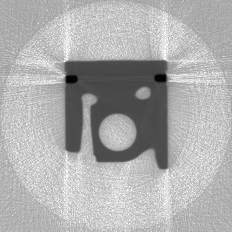
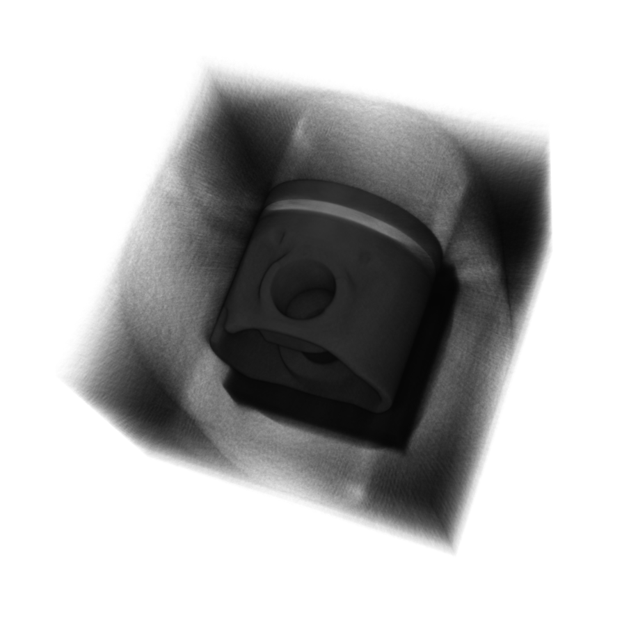
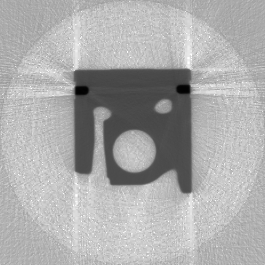
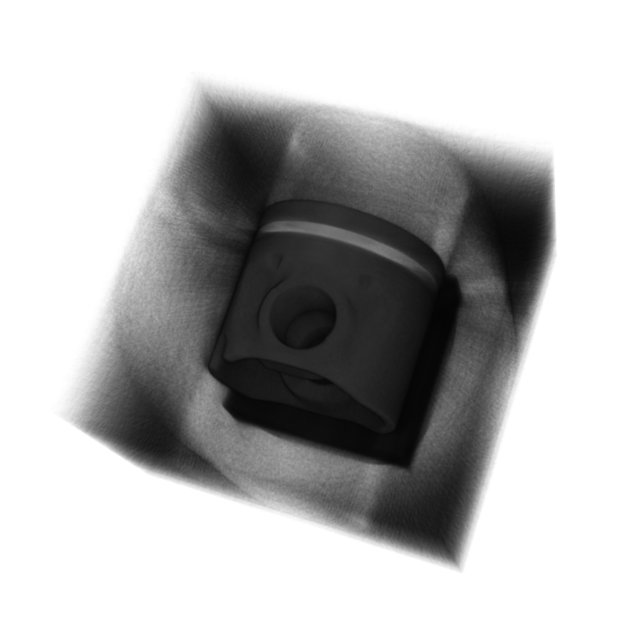
Figure 5: Left column: slice views. Right column: 3D views. Top row: LiveTV regularization results. Bottom row: SparseTV regularization results. In all cases, the parameter $\lambda=10^{3}$ is used. Gamma correction was applied to highlight the noise details.

 

 

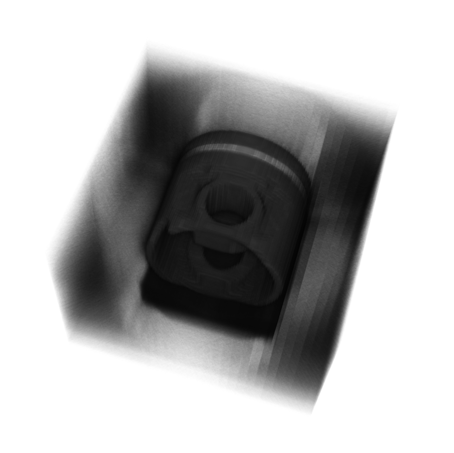
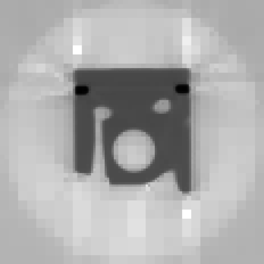
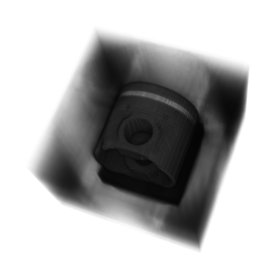
Figure 6: Left column: slice views. Right column: 3D views. Top row: LiveTV regularization results. Bottom row: SparseTV regularization results. In all cases, the parameter $\lambda=10^{5}$ is used. Gamma correction was applied to highlight the noise details.

Fig. 5 and 6 indicate that, for larger thresholds, the reduction of noise texture is stronger when using SparseTV while the image quality at material transitions is comparable. The three-dimensional views show similar noise texture properties.

 

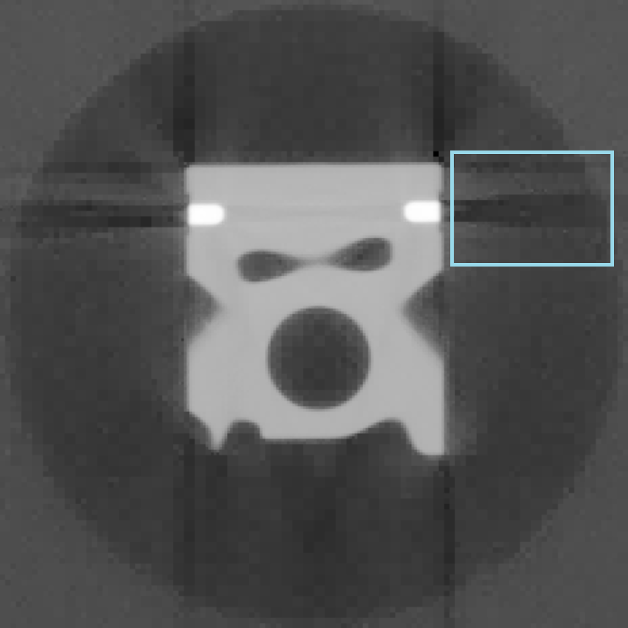
Figure 7: Left: motor piston slice after hard thresholding, exhibiting speckle-like noise in different resolutions, for example in the top-right corner. Right: motor piston slice after SparseTV with more resolution-consistent noise and the same resolution at the important edges at the borders between air and aluminum, for example, in the circular part in the middle. Gamma correction was applied to both images to highlight the noise details.

In this practical example, SparseTV also leads to less fluctuations regarding the surrounding noise compared to classical thresholding, where the coefficients are manipulated independently, which can be seen in Figure 7.

 

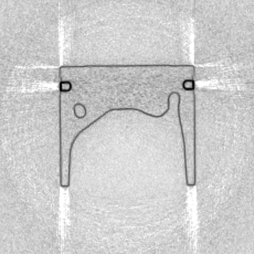
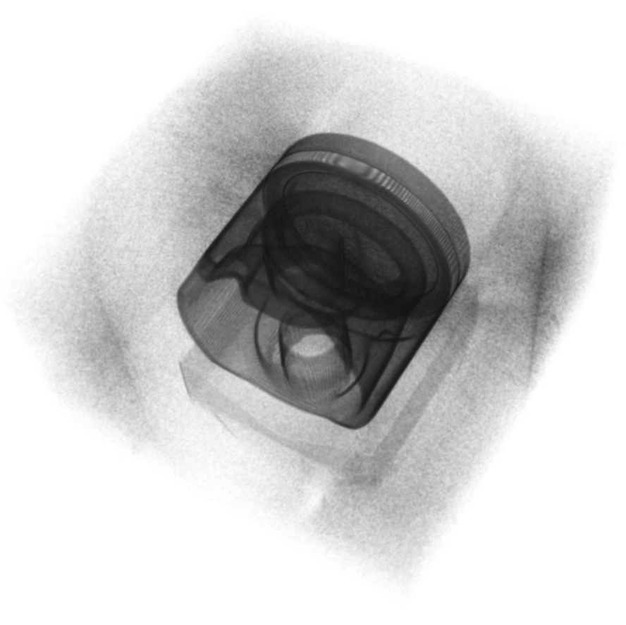
Figure 8: Slice and three-dimensional view of the motor piston wavelet gradient approximations with additional gamma correction, logarithmic scaling and thresholding to balance visibility of material transitions and noise.

Finally, the single-wavelet-component coefficients can be used for approximating the gradients, as shown above. However, it was not possible to visually detect manufacturing errors, possibly due to the halved gradient resolution, see Fig. 8.

References

- [1] A. Chambolle, V. Caselles, D. Cremers, M. Novaga, and T. Pock, An introduction to total variationfor Image Analysis, in Theoretical Foundations and Numerical Methods for Sparse Recovery, M. Fournasier, ed., vol. 9 of Radon Series Comp. Appl. Math, De Gruyter, 2010, pp. 263–340, https://doi.org/10.1515/9783110226157.263.
- [2] B. Diederichs, T. Sauer, A. M. Stock, Mathematical aspects of computerized tomography: compression and compressed computing, Fifteenth International Conference Zaragoza-Pau on Mathematics and its Applications, 42 (2019), pp. 79–93.
- [3] A. Haar, Zur Theorie der orthogonalen Funktionensysteme, Math. Ann., 69 (1910), pp. 331–371.
- [4] G. G. Lorentz, Approximation of Functions, Chelsea Publishing Company, 1966.
- [5] S. Mallat, A Wavelet Tour of Signal Processing: The Sparse Way, Academic Press, 3rd ed., 2009.
- [6] Y. Meyer, Wavelets – Algorithms and Applications, SIAM, 1993.
- [7] R. Reisenhofer, S. Bosse, G. Kutyniok, and T. Wiegand, A haar wavelet-based perceptual similarity index for image quality assessment, Signal Proc. Image Comm., 61 (2018), pp. 33–43.
- [8] R. T. Rockafellar, Convex Analysis, Princeton University Press, 1970.
- [9] L. I. Rudin, S. Osher, and S. Fatemi, Nonlinear total variation based noise removal algorithms, Physica D, 60 (1992), pp. 259–268.
- [10] M. Salamon, N. Reims, M. Böhnel, K. Zerbe, M. Schmitt, N. Uhlmann, and R. Hanke, XXL-CT capabilities for the inspection of modern electric vehicles, International Symposium on Digital Radiology and Computed Tomography – DIR 2019, (2019).
- [11] G. Steidl and J. Weickert, Relations between soft wavelet shrinkage and total variation denoising, in Pattern Recognition. DAGM 2002, L. V. Gool, ed., vol. 2449 of Lecture Notes in Computer Science, Springer, 2002.
- [12] A. M. Stock, G. Herl, T. Sauer, and J. Hiller, Edge preserving compression of CT scans using wavelets, Insight, 62 (2020), pp. 345–351, https://doi.org/10.1784/insi.2020.62.6.345.
- [13] M. Welk, G. Steidl, and J. Weickert, Locally analytic schemes: A link between diffusion filtering and wavelet shrinkage, Appl. Comput. Harmon. Anal., 24 (2008), pp. 195–224, https://doi.org/10.1016/j.acha.2007.05.004.