Alfvénic waves in the inhomogeneous solar atmosphere

Abstract

The solar atmosphere is known to be replete with magneto-hydrodynamic wave modes, and there has been significant investment in understanding how these waves propagate through the Sun’s atmopshere and deposit their energy into the plasma. The waves’ journey is made interesting by the vertical variation in plasma quantities that define the solar atmosphere. In addition to this large-scale inhomogeneity, a wealth of fine-scale structure through the chromosphere and corona has been brought to light by high-resolution observations over the last couple of decades. This fine-scale sturcture represents inhomogeneity that is thought to be perpendicular to the local magnetic fields. The implications of this form of inhomogeneity on wave propagation is still being uncovered, but is known to fundamentally change the nature of MHD wave modes. It also enables interesting physics to arise including resonances, turbulence and instabilities. Here we review some of the key insights into how the inhomogeneity influences Alfvénic wave propagation through the Sun’s atmosphere, discussing both inhomogeneities parallel and perpendicular to the magnetic field.

1 Introduction

Ever since it was established that the coronal plasma had temperatures in excess of a million degrees (based on the emission lines from forbidden transitions of highly ionized atoms, Grotian 1939; Edlén 1941; Alfvén 1941; Edlén 1943), heating of the Sun’s atmosphere or corona has remained an intriguing problem in solar and stellar astronomy. As one of the promising answers to this dilemma, Alfvénic waves have long attracted the attention of the community as a mechanism that could not only answer the coronal heating but can also explain the acceleration of solar wind (e.g., Arregui 2015; Van Doorsselaere et al. 2020b). A particular reason for the interest in this wave mode, as compared to the other magnetohydrodynamic (MHD) waves, is it’s highly incompressible nature that makes it difficult for the Alfvénic waves to dissipate their energy. This property enables these waves to transfer the mechanical energy from the photosphere, where they are generated via the interaction of the magnetic fields with the convective motions, up into the corona and out into the heliosphere. However, the journey of the Alfvénic waves through the Sun’s atmosphere is not straightforward, with the inhomogeneous nature of the plasma leading to many interesting wave-related phenomena. Here we do not just refer to inhomogeneities along the magnetic field, but also the fine-scale perpendicular structuring that is observed throughout the chromosphere and corona.

An example of such perpendicular structuring is visible in the Extreme Ultra-Violet (EUV) image of the corona from NASA’s Solar Dynamic Observatory (SDO) displayed in Figure 1. Present in the image are: a myriad of loop-like structures that emanate from the Active Regions; comparatively fainter loops in the quiet Sun (best seen off-limb) that are the base of larger structures extending into the heliosphere (e.g., streamers, pseudo-streamers); and near-radially oriented striations extending out of the field of view in the quiet Sun and polar regions (again best seen off-limb). The visibility of these structures is thought to be due to an excess of density relative to the ambient plasma, highlighting collections of magnetic field lines. The density enhancements are possibly due to local heating events associated with the magnetic fields (e.g., Cargill 1994; Yokoyama & Shibata 2001; Gudiksen & Nordlund 2005; Klimchuk et al. 2008).

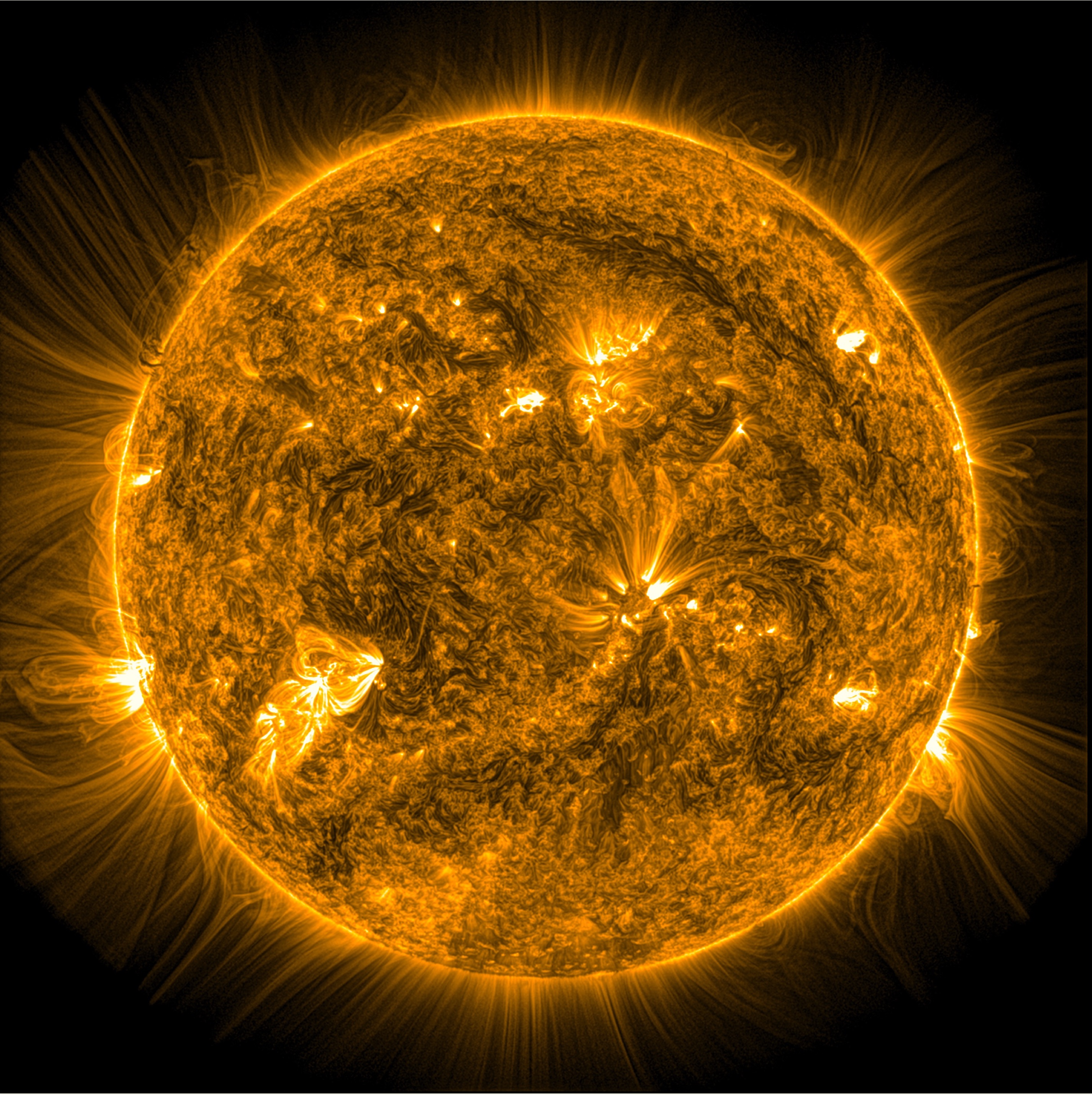
Figure 1: An EUV image of the Sun’s corona taken with the Solar Dynamic Observatory. The image reveals the fine-scale striations throughout the upper layer of the Sun’s atmosphere, indicating the highly inhomogeneous nature of the coronal plasma. The dynamic range of the image has been altered to enable the faint plasma emission around the limb to be visible.

Past efforts have placed significant attention upon understanding the influence of an inhomogeneous plasma on Alfvénic wave propagation. However, this has, until recently, been largely split into distinct areas of focus. One of these areas was predominantly interested in modelling the impact of Alfvénic waves on the solar wind (for reviews see, e.g., Bruno & Carbone 2005; Cranmer et al. 2017), and hence focused on the inhomogeneity along the magnetic field, though a number of studies attempt to include the influence of the lower solar atmosphere as well. However, others were particularly interested in the role of perpendicular structuring, driven primarily by interests in wave heating of coronal loops (for reviews see, e.g., Arregui 2015; Nakariakov & Kolotkov 2020). The final camp focused on wave propagation through partially ionized plasmas, investigating the role of ion-neutral effects (for a review, see, e.g., Ballester et al. 2018). The division into these areas is, in part, due to the vast range of scales that would be required to incorporate all the vital physics from the photosphere to the corona (and beyond). However modern numerical resources are enabling these areas to draw closer together. We should mention that a number of works that have sought to bring together inhomogeneity parallel and perpendicular to the magnetic field. The studies where largely focused on emulating and predicting properties of strongly damped resonant coronal loop oscillations (starting with, e.g., Andries et al. 2005b, a; Verth 2007; Verth et al. 2007), and the opportunities for magneto-seismology (see, e.g., Andries et al. 2009; Nakariakov et al. 2021, for related reviews).

In the following we aim to provide an overview on the role inhomogeneities play in Alfvénic wave propagation. The phenomenon we discuss are likely to be present across the solar atmosphere, although the specifics (e.g., associated time-scales, magnitudes) of the wave generation, propagation and dissipation will depend upon the local plasma conditions. However, to bring together the details, it is necessary to outline a stage upon which wave propagation and evolution takes place. Here we will focus on wave propagation in the quiescent Sun and coronal holes, and largely avoid active regions. This choice is mainly driven by the fact that the magnetic structure and plasma conditions in the quiescent Sun and coronal holes are similar, at least in the lower solar atmosphere. Further, active regions are relatively infrequent features on the Sun when compared to the quiet Sun. Hence, the description of wave propagation in the quiet Sun provides a more general picture. This is not to say that the details of Alfvénic waves in active regions are unimportant or uninteresting, far from it. We also note that in some of the given references, the analytic and numerical results are tailored to plasma conditions thought to be representative of coronal loops in active regions. Hence, it should be kept in mind that the numerical values given in those papers with respect to the phenomenon under study will need to modified for the quiet Sun.

1.1 Basic structure of the solar atmosphere

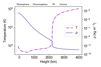
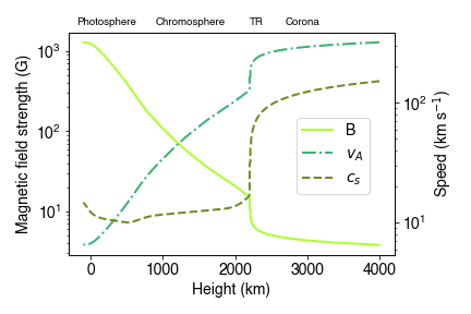
Figure 2: A descriptive model of the solar atmosphere. The left panel shows temperature and density profiles. The lower solar atmosphere up to $\sim 2000$ km is based on the FAL quiet Sun model (see text) and an additional coronal extension. The right hand panel displays an empirical magnetic field model for a magnetic bright point with a photospheric field strength of 1300 G. The corresponding Alfvén and sound speeds for the model atmosphere are also shown.

To highlight some of the key inhomogeneities that affect the Alfvénic waves, it is worth providing a description of the basic structure of the Sun’s atmosphere. The left panel of Figure 2 shows the temperature and mass density profiles as a function of height in the lower solar atmosphere, from photosphere to the coronal base. The atmospheric profile shown is from a series of models by Fontenla et al. (1993), of which we select the quiet Sun profile (referred to as the FAL-C model). The FAL model is extended into the corona following Soler et al. (2017) with an assumption of a fully ionised corona.

As noted by Rutten (2021), it is worth recognising that the FAL models really only represent the atmosphere of a solar-analog. The atmosphere in these models is 1D plane parallel with no magnetic field and lacking any of the dynamics that are observed (e.g. waves, shocks, granulation, spicules). However, the FAL models (and the earlier VAL versions Vernazza et al. 1981) are a vital starting point for many investigations into wave propagation through the atmosphere of a Sun-like star. With this in mind, it can be seen that the temperature and density are expected to continuously vary with height. To complement the temperature and density, Figure 2 also shows an empirical model for the variation in vertical magnetic field strength (Leake et al. 2005). The shown magnetic field profile should represent the expanding magnetic field emanating from intense magnetic flux tubes embedded in the photosphere (known as magnetic bright points due to their appearance in certain photospheric diagnostics, e.g., Berger & Title 1996; Tsuneta et al. 2008; de Wijn et al. 2009; Ito et al. 2010). In combination with the mass density, one can estimate the Alfvén speed ($v_{A}=B/\sqrt{\mu_{0}\rho}$) profile through the atmosphere (and using the prescribed temperature profile we also provide the sound speed, $c_{s}$, profile).

For the Alfvénic wave propagation, the temperature structure is usually not a major consideration due to the highly incompressible nature of the waves (although will play a role in the story, e.g., through its influence on the ionisation state of the plasma - Section 5.1). Of particular importance is the mass density, and to a degree the magnetic field, which shapes the details of the waves’ journey through different layers of the stratified solar atmosphere. It can be seen in Figure 2 that the mass density has a scale height of 100-200 km in the lower solar atmosphere, which leads to a rapid increase in Alfvén speed. To conserve wave energy flux ($F=\frac{1}{2}\rho v^{2}v_{A}$), this leads to wave amplification, which can then induce non-linear mode coupling and shocks (discussed in Section 5). Upwardly propagating waves then encounter the sharp change in density that occurs at the transition region, which acts as a frequency filter and is a decisive factor in determining the Alfvénic wave energy that is able to enter the corona. The change in Alfvén speed in the corona and above is much more gradual, although it no less interesting; it is a key factor in the development of turbulence (Section 4.3).

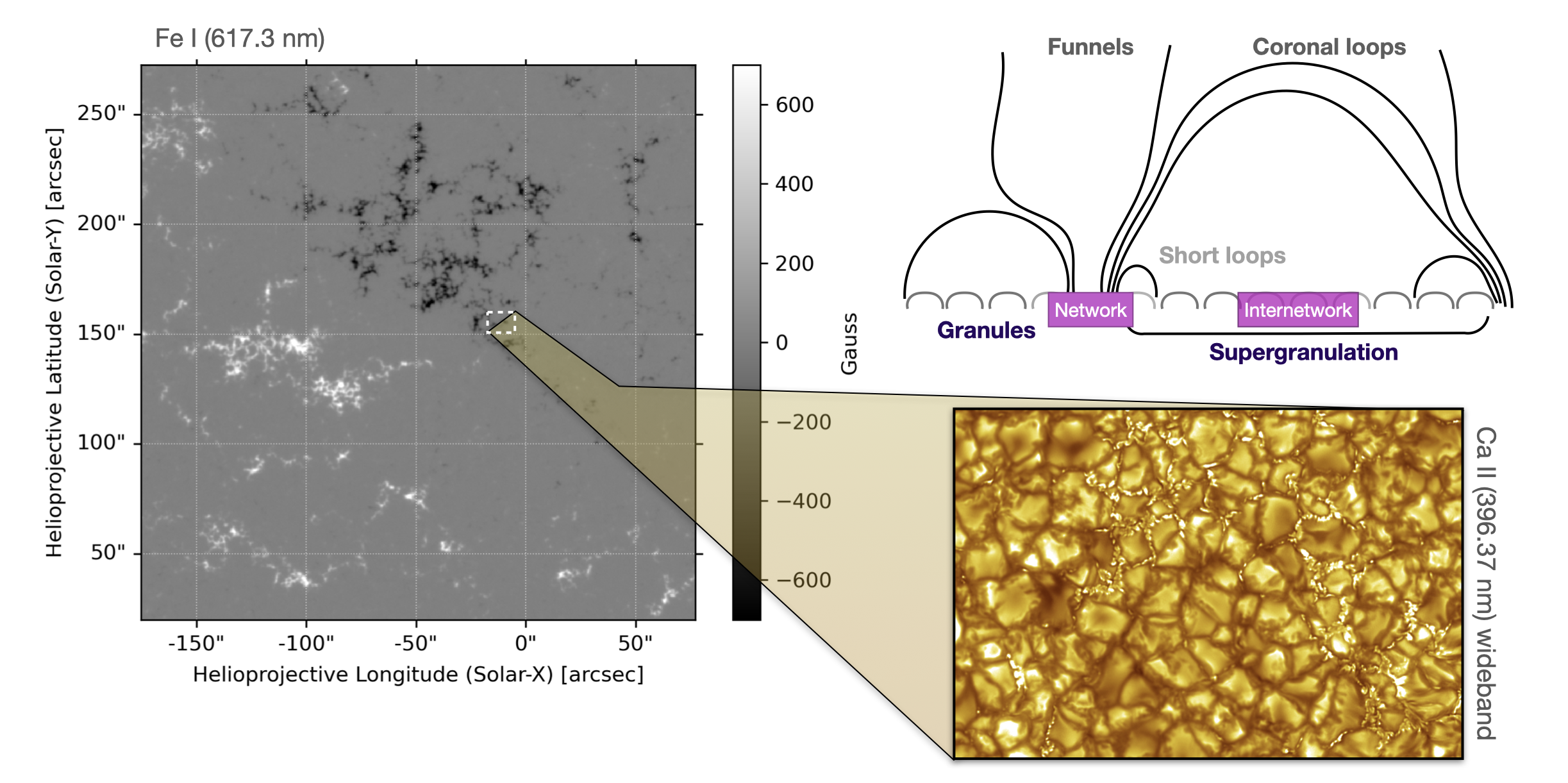
Figure 3: A sketch of the organisation of the magnetic field in the quiet Sun. The left hand image is the photospheric magnetic field measured from the Zeeman splitting on an Fe I line (a magnetogram) by the Heliosesmic & Magnetic Imager onboard SDO. The central feature of the image is relatively large clusters of magnetic field that highlight the network. The bottom right panel shows a small portion of the network, revealing the small-scale magnetic flux features as bright points (image courtesy of V. Henriques, taken with the Swedish Solar Telescope operated by Institute for Solar Physics, Stockholm, Sweden).

1.2 The large-scale organisation of the magnetic field

The large-scale organisation of the magnetic field plays an important role in characterising the spatial and temporal evolution of waves in the solar atmosphere. Hence, we believe it is important to overview critical aspects of this element here. A complete assessment, however, will require many more pages though we direct an avid reader to many other excellent texts discuss the structure, dynamics and evolution, (e.g., Schrijver & Zwaan 2000; de Wijn et al. 2009; Bellot Rubio & Orozco Suárez 2019).

The organisation of the magnetic field depends upon height in the solar atmosphere, but is ultimately engendered by its distribution in the photosphere. The gas density and temperature vary by orders of magnitude between the photosphere and the corona, with the dynamics of the plasma controlling the evolution of the field in the photosphere (ratio of plasma pressure to magnetic pressure, or plasma beta, being greater than 1). Eventually, the rapid decrease in plasma pressure means that the magnetic field begins to dominate both the appearance and dynamics in the upper chromosphere and beyond (where plasma beta is less than 1).

At the photospheric level, the magnetic field is found to emerge as (or coalesce into) small, intense kilogauss elements concentrated in the lanes between the granules (these magnetic bright points are seen in the Ca II image in Figure 3). Over time, many of these small elements are advected to the edges of the so-called network (Zirin 1985; Suárez et al. 2012; Gošić et al. 2014), which is thought to highlight the lanes of a super-granular flow pattern deep in the interior (Figure 3). This produces a large-scale ($\sim 15-30$ Mm) patchwork of magnetic field (November & Simon 1988; De Rosa & Toomre 2004), although is still made up from clusters of small-scale magnetic elements (see the magnetogram in Figure 3). The small-scale elements within the interior of the network (or internetwork) are generally thought to be the foot-points of low-lying, closed magnetic fields, extending only as high as the chromosphere and transition region (González & Rubio 2009; Wiegelmann et al. 2010). In contrast, those magnetic fields at the network boundaries extend into the upper atmosphere, spreading out as the gas pressure falls off and eventually filling the volume of the corona. In the upper right panel of Figure 3 we sketch this scenario. These magnetic fields are then either closed, connecting with opposite polarity flux and spanning the internetwork region; or they are open funnels, connected to the solar wind (more detailed discussions can be found in, e.g., Peter 2001; Wedemeyer-Böhm et al. 2009). The separation of network and internetwork fields is likely not so neat, with the potential for short loops to exist with a foot-point in both (Wiegelmann et al. 2010) and internetwork fields also contributing to the funnels.

1.3 The fine-scale structure

Near the top of the chromosphere, the magnetic field begins to dominate both the appearance and dynamics of the solar atmosphere. As mentioned, the plasma beta is much less than one in these regions. This is complemented by high magnetic Reynold’s number ($\gg 1$), meaning that the magnetic field obeys the so called ‘frozen-in’ condition which prohibits the cross-field diffusion of the plasma. Heating events can lead to evaporation or injection of plasma into the upper parts of the atmosphere and the consequence of the ‘frozen-in’ condition is that the plasma is confined to move along the magnetic field lines. This leads to enhancements of density along bundles of magnetic field lines, and provides the fine-scale structure seen in many images of the chromosphere and corona (e.g., Figure 1). The fine-structure has many forms, from elongated chromospheric fibrils and coronal loops, to short and highly dynamic spicules that originate in the chromosphere. The fibrils, spicules (e.g., Rutten 2007; Tsiropoula et al. 2012; Jess et al. 2015; Carlsson et al. 2019) and active region coronal loops (e.g., Reale 2014) have been well-studied . However, many of the other density striations seen in Figure 1, e.g., quiescent coronal loops and the near radial features in polar coronal holes, are presently little-studied.

In both the chromosphere and corona, the well-studied structures have widths down to the resolution of current instrumentation; with typical widths around $\sim 200-300$ km (e.g. Antolin & van der Voort 2012; Pereira et al. 2012; Brooks et al. 2013; Morton & McLaughlin 2014). Estimates for the over-density of some of these features, namely coronal loops in active regions, has been possible. For example, Aschwanden et al. (2000) suggests the density of warm coronal loops is an order of magnitude more than that expected from hydrostatic equilibrium, which the ambient plasma is expected to be in. More recently, Pascoe et al. (2017) use seismology and estimate over-density values in the range 1.5-5.

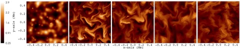
Figure 4: The destruction of simplified loop geometries. The figure shows the cross-sections of coronal loops, displaying the density. The magnetic field is orientated perpendicular to the 2D slice shown. The loops are initially over-dense with a Gaussian density profile in the cross-section (left hand panel), which gradually becomes distorted over time. The time step between panels is 250 s and the density colour-bar is shown in units of $10^{-12}$ kg m^-3. Figure reproduced from Magyar et al. (2017).

Apart from the density and cross-sectional width of fine-scale structures, another noteworthy aspect is the cross-sectional geometry of the flux tubes in the solar atmosphere. Parker (1974a, b) suggested cylindrical geometry of these features using a simplistic hydrodynamic mechanism involving turbulent pumping to coalesce magnetic fields into the slender, tube-like structures. This simplified assumption remained a cornerstone to the wave studies in localised chromospheric and coronal structures (e.g., Goossens et al. 2011). However, there has been some work that has ventured from this assumption, (e.g., Morton & Erdélyi 2009; Pascoe et al. 2011; Morton & Ruderman 2011; Guo et al. 2020). The observational evidence for the actual cross-sectional geometry of the chromospheric and coronal structures is scant. Theoretical work suggests that the shape of the flux tube cross section can vary along the structure, and is likely oblate (Ruderman 2009; Malanushenko & Schrijver 2013). Observational studies are particularly complex, and appear to show mixed results (McCarthy et al. 2021). Moreover, recent simulations have demonstrated that, even when starting with circular cross-sections, the presence of transverse waves lead to a distortion of the flux tubes cross-section through instabilities (e.g., Antolin et al. 2014; Magyar & Van Doorsselaere 2016; Magyar et al. 2017; Antolin & Van Doorsselaere 2019, and discussed further in Section 4.2). Figure 4 shows simulation results from Magyar et al. (2017) that demonstrate this process in action.

Furthermore, it has been speculated that the appearance of a near-circular tube-like geometry of the fine-scale structures could be due to observational artefacts. Judge et al. (2011) suggested that some observed chromospheric spicular structures are wrapped current sheets that appear as thin, elongated features. More recently, Malanushenko et al. (2022) put forward the idea that some bundles of coronal loops are optical illusions in EUV passbands. The authors suggest that these features are actually complex and diffuse objects (‘wrinkles in the coronal veil’) that appear as compact, slender structures due to artifacts that arise from the inherent integration along the line of sight over extended regions in optically thin plasma. The authors examined the coronal structures using highly realistic numerical simulations, and found that the cross-sections of many coronal structures appear to show a highly turbulent appearance (similar to the cross-sections from Magyar et al. 2017 shown in Figure 4). However, it is not discussed how or why the corona is structured in such away.

Importantly, while the actual cross-sectional shape of flux tubes is unknown, both observations and simulations suggest that there are plasma inhomogeneities in the direction perpendicular to the magnetic field. As we shall now discuss, this enables a wealth of interesting wave physics to take place and is likely a key factor in enabling the dissipation of wave energy in the chromosphere and corona.

2 Linear Alfvén Wave Theory

To appreciate the impact of an inhomogeneous plasma on wave propagation, we briefly discuss some of the fundamental theoretical aspects of linear Alfvénic waves in a structured plasma. It turns out that perpendicular inhomogeneity in the plasma modifies the classical picture of wave behaviour presented in the textbook examples of homogeneous plasma, and removes the clear division between Alfvén and magneto-sonic modes. It was noted as early as 1982 by Hasegawa & Uberoi (1982) that the presence of inhomogeneity leads to coupling of the total pressure to the dynamics for Alfvén modes. Inhomogeneity also enables the MHD waves to have a different appearance in different parts of the plasma, readily modifying their dominant characteristics. The following aims to be a discussion of the salient points, and we recommend readers refer to the original texts for deeper discussions (e.g., Hasegawa & Uberoi 1982; Goossens 2003; Goossens et al. 2012, 2019). We first discuss the case of a homogeneous plasma before moving onto the more interesting physics that occurs when this restriction is dropped.

2.1 The homogeneous case

To begin, let us assume that we have a plasma with magnetic field that is oriented in the $z$ direction and is homogeneous in all plasma quantities along the field. We make no assumptions about the plasma perpendicular to the field at this moment. The linearised ideal MHD equations can be reduced to (e.g., Goossens et al. 2012),

$$\omega^{2}\xi_{z}-k_{z}c_{s}^{2}Y = 0,$$ (1)

$$k^{2}v_{A}^{2}k_{z}\xi_{z}+(\omega^{2}-k^{2}(c_{s}^{2}+v_{A}^{2}))Y = 0$$ (2)

$$(\omega^{2}-k_{z}^{2}v_{A}^{2})Z = 0,$$ (3)

for planar, harmonic waves, i.e., wave variables are proportional to $\exp(ik_{z}z-i\omega t)$, where $\omega$ is the frequency and $k_{z}$ is the longitudinal wave number. Here the equations have been expressed in terms of variables that expose the underlying physics. The variables are the magnitude of the wavevector $k=\sqrt{k_{x}^{2}+k_{y}^{2}+k_{z}^{2}}$, the sound speed $c_{s}$, the Alfvén speed $v_{A}$, and the Lagrangian displacement along the magnetic field, $\xi_{z}$. Additionally, we have also used the plasma compression,

$$Y=-i\nabla\cdot\vec{\xi},$$ (4)

and the vorticity parallel to the magnetic field,

$$Z=-i(\nabla\times\vec{\xi})_{z},$$ (5)

where $\vec{\xi}$ is the Lagrangian displacement vector. It is also useful to define the ratio of the horizontal components of the total pressure force and the magnetic tension force (Goossens et al. 2012), which is given by,

$$\Lambda(\omega^{2})=\frac{\omega^{2}}{(k_{z}v_{A})^{2}}-1.$$ (6)

In an homogeneous media of infinite extent, the system of equations (1)-(3) are decoupled into two systems. One of these describes Alfvén waves and contains only the vorticity along the field, i.e., Eq. 3. There is no compression or displacement along the magnetic field ($Y=0$, $\xi_{z}=0$). The solution to this set of equations results in the well known dispersion relation,

$$\omega=k_{z}v_{A}.$$

Hence, from Eq. 6 it can be found that $\Lambda(\omega^{2})=0$, and magnetic tension is the only restoring force. The other system involves the variables $\xi_{z}$ and $Y$, and defines the magneto-sonic modes, i.e., Eqs. 1 and 2. Unlike the Alfvén waves, these magneto-sonic modes are compressible and have a longitudinal displacement but do not propagate parallel vorticity.

2.2 Perpendicular inhomogeneities

The addition of an inhomogeneity in the direction perpendicular to the magnetic field leads to a coupling of the wave variables, which, in the case of a straight magnetic field, is mediated by Eulerian perturbation of the total pressure (for a twisted field there is a stronger coupling arising from the so-called coupling functions, e.g., Sakurai et al. 1991; Goossens et al. 2019). This coupling leads to MHD waves having mixed properties and is present even in the linear MHD system (e.g., Goossens et al. 2002). There are two scenarios that are worth discussing as they highlight key aspects of increasing the geometric complexity.

The first case of interest is two uniform plasma separated by a discontinuity in the Alfvén velocity, which we can assume arises due to a discontinuity in the density, i.e.,

$$\rho(x)=\begin{cases}\rho_{i}&\hskip 14.22636ptx\leq x_{0},\\ \rho_{e}&\hskip 14.22636ptx>x_{0}.\end{cases}$$

At such an interface, Alfvén surface modes are able to exist (Wentzel 1979b, a; Roberts 1981). In the limit of ‘nearly perpendicular propagation’ ($k_{y}^{2}>>k^{2}_{z}$), the dispersion relation for the surface mode is given by:

$$\omega^{2}=k_{z}^{2}\frac{\rho_{i}v^{2}_{Ai}+\rho_{e}v^{2}_{Ae}}{\rho_{i}+\rho_{e}}\equiv\omega_{k}^{2},$$ (7)

which lies between the Alfvén frequencies for both plasmas. Hence, $\Lambda$ (given in Eq. 6) is small on either side of the discontinuity and magnetic tension dominates the restoring forces. The surface mode is also largely insensitive to the value of the sound speed. Furthermore, it has the property that parallel vorticity is zero everywhere except at the discontinuity, contrary to the classical Alfvén wave in uniform plasma (Goossens et al. 2012). For such a mode, an appropriate term is Alfvénic, which highlights such modes are different from the classical Aflvén wave, and has mixed properties.

The second case is that of a 1D magnetic cylinder, which we describe in cylindrical coordinates, ($r$, $\theta$, $z$). The magnetic field is still oriented in the $z$ direction. Since the background plasma depends only on perpendicular inhomogeneities, which are in the radial ($r$) direction, then the perturbations, independent of azimuth ($\theta$) and $z$, are proportional to

$$\exp(i(m\theta+k_{z}z-\omega t)),$$

where $m$ is the azimuthal wavenumber. In this case, Eqs. 4 and 5 become

$$Y=\frac{1}{r}\frac{\partial(r\xi_{r})}{\partial r}+im\xi_{\theta}+ik_{z}\xi_{z},\hskip 28.45274ptZ=\frac{1}{r}\frac{\partial(r\xi_{\theta})}{\partial r}-im\frac{\xi_{r}}{r}.$$

For the case of $m=0$, it can be seen from these expressions for $Y$ and $Z$ that Eqs. 1-3 are decoupled. The solutions to the two sets of equations are axisymmetric modes, namely the torsional Alfvén mode and the sausage magneto-sonic mode. The Alfvén mode depends only upon $\xi_{\theta}$, as each magnetic surface oscillates at its own frequency. As noted by Goossens et al. (2019), this is the only pure Alfvén mode in a non-uniform 1D cylindrical plasma. The nature of the coupling is further elucidated by the coupling function derived by Sakurai et al. (1991) for a straight magnetic field, namely,

$$C_{A}=\frac{m}{r}B_{z}P^{\prime},$$ (8)

where $P^{\prime}$ is the total pressure perturbation. It can be seen that a total pressure perturbation is also required to be non-zero in order for coupling, as well as $m\neq 0$.

Under the simplifying assumption of a magnetic flux tube with a piece-wise constant density (e.g., Spruit 1982; Edwin & Roberts 1983), solutions exist for any $m$ that can be identified with Alfvén waves (i.e., solutions with $\nabla\cdot\vec{v}=0$). More generally, for any geometry, a pure Alfvén mode can exist if there is an ignorable transverse direction. However, in the non-uniform 1D cylinder, modes with $m\neq 0$ have mixed properties and all wave variables are coupled. All eigenmodes of the system now have all perturbed quantities that are non-zero (Goossens et al. 2002, 2019). Here, the modes cannot be separated by the distinctions found in the homogeneous case. Also of interest, it turns out all wave modes in inhomogeneous plasma are efficient generators of vorticity (Goossens et al. 2019).

Before moving on, it is worth mentioning the non-axisymmetric kink mode (when $m=1$) in detail. This particular wave mode has been the subject of great interest over the last two decades. Transverse oscillations of coronal loops, first noticed in observations back in the 1990’s, were interpreted as the kink mode (Aschwanden et al. 1999; Nakariakov et al. 1999). Then, after observations of transverse waves in the chromosphere (De Pontieu et al. 2007; Okamoto et al. 2007) and corona (Tomczyk et al. 2007) in 2007, the kink mode was subject to an intense discussion about the wave properties and nomenclature. In one of the seminal papers on MHD waves in flux tubes, Edwin & Roberts (1983) used the prefix ‘fast’ to describe the mode. As mentioned, the solar atmosphere is highly inhomogeneous and MHD waves in this environment portray mixed properties and it is misleading for the modes to be classified using the labels derived from the homogeneous case (Goossens et al. 2019).

The characteristics of the kink mode were examined and discussed in detail by Goossens et al. (2009), where they demonstrated that the kink mode is in fact very robust and cares little for the plasma environment when $k_{z}R<1$ (here, $R$ is the flux tube’s radius). Moreover, the kink mode was shown to be highly incompressible, with negligible pressure perturbations. The dispersion relation for the kink mode in a cylinder with a piece-wise constant density is given by Eq. 7, while the ratio given by Eq. 6 is

$$\Lambda_{i}(\omega)=-\Lambda_{e}(\omega)=\frac{\rho_{i}-\rho_{e}}{\rho_{i}+\rho_{e}},$$

in the interior and exterior of the cylinder. Hence, for any value of density contrast, this ratio is always less than one and magnetic tension is the dominant restoring force. This led Goossens at al. to suggest the descriptor for these waves should be Alfvénic, alluding to the dominant properties being close to classical Alfvén wave. In a follow up work, Goossens et al. (2012) go onto to demonstrate that the fundamental radial modes for any non-axisymmetric wave mode ($m>0$) can be described as a surface Alfvén wave. In this case, the waves display the same properties as a surface Alfvén wave at a true discontinuity. However, if the discontinuity is replaced by a region of non-uniform, continuously varying density, then the vorticity is present throughout this region and the modes are Alfvénic global/quasi modes(Goossens et al. 2002). The presence of vorticity and the continuously varying density profile leads to a number of interesting effects that impact wave propagation, damping, and dissipation; which are discussed in section 4.

3 Wave excitation

Recent theoretical models have shown that the inhomogeneous nature of the Sun’s atmosphere could also play a key role in exciting Alfvénic waves. We first overview the existing paradigm surrounding the excitation of Alfvénic waves and then discuss mode conversion from inhomogeneities.

3.1 Convection

The typical picture of Alfvénic wave generation begins at the photosphere and was suggested many decades ago (e.g., Osterbrock 1961). The turbulent patterns of granulation are the most common feature of the photospheric topology (Figure 3), that manifest from the convective motions deep within the solar interior. The average lifetime of granular cells is 5-10 minutes and have horizontal scales of about 1 Mm (e.g., Schrijver et al. 1997). As mentioned in Section 1, the boundaries of these granular cells appear as dark lanes where strong plasma downflows are observed. These intergranular lanes form favourable sites for harbouring intense concentrations of magnetic flux known as magnetic bright points (MBPs). The MBPs are seen to be passively advected with the large-scale super-granule flow but are also subject to buffeting from the granulation (Berger & Title 1996; Berger et al. 1998; van Ballegooijen et al. 1998; Nisenson et al. 2003; Chitta et al. 2012). The associated horizontal motions are turbulent and rapid, with an average root-mean-squared (RMS) velocity of $\sim 1-1.5$ km/s and correlation times of 20-30 s (Chitta et al. 2012), while the line-of-sight (LOS) Doppler velocity magnitudes are of the order $\sim$1.2 km/s (Nordlund et al. 2009; Oba et al. 2017).

These motions correspond to the both horizontal and vertical shaking of the magnetic bright points and can induce various types of MHD wave-like fluctuations at the foot-points of thin magnetic flux tube structures (Spruit 1981; Steiner et al. 1998). While vertical motions can drive sausage or longitudinal modes (Defouw 1976; Roberts & Webb 1978), the horizontal motions can induce transverse waves, namely the kink mode, if using a flux tube description for the bright points (Spruit 1981; Choudhuri et al. 1993; Musielak & Ulmschneider 2002). Cranmer & van Ballegooijen (2005) suggested such kink modes would convert to ‘classical’ Alfvén waves in the low chromosphere when the individual magnetic elements expand and merge with one another. This implies that the upper atmosphere is homogeneous perpendicular to the magnetic field (as is the case of the Cranmer & van Ballegooijen model). However, as discussed in the introduction, the chromosphere and corona apparently possess a significant amount of inhomogeneity. Hence, the wave energy should propagate to upper layers as Alfvénic modes instead - although we are unaware of any model/theory that addresses the details of how this may happen.

Closely related to the horizontal motions are photospheric vortices, which are convective down-drafts in the intergranular lanes. They were initially detected through the observed motions of MBPs (Bonet et al. 2008) and have been found to be ubiquitous across the photosphere (e.g., Wedemeyer-Böhm & Rouppe van der Voort 2009; Morton et al. 2013; Giagkiozis et al. 2018; Liu et al. 2019) and in numerical simulations (e.g., Shelyag et al. 2011; Moll et al. 2011). Such vortices appear to be capable of exciting rotational Alfvénic modes in numerical simulations (Battaglia et al. 2021; Breu et al. 2022), and have also been suggested to enable distortions of flux elements shape and intermixing of field lines, leading to MHD wave excitation (van Ballegooijen et al. 2011).

3.2 Mode conversion

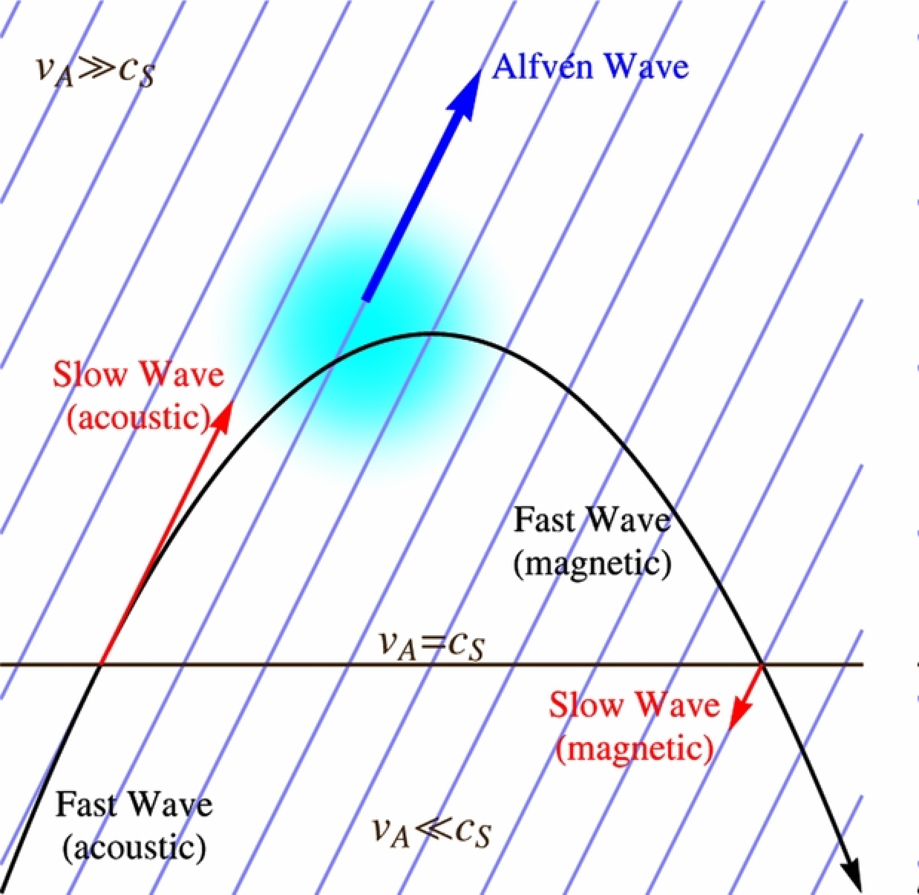
Figure 5: A sketch of the double mode conversion in the lower solar atmosphere that ends in the production of Alfvénic waves. The details are discussed in the text. The blue diagonal lines represent the magnetic field. Reproduced from Khomenko & Cally (2012) permission of the AAS.

More recently, there has been interest in alternative pathways for convective energy to reach the corona as Alfvénic waves. In part this interest has been driven by some fundamental theoretical results (Cally & Goossens 20008), but also by the apparent high reflectivity of the transition region to photospheric driven Alfvénic waves (suggested to be $\sim 95$ % reflection rate by Cranmer & van Ballegooijen 2005). The essence of this pathway is shown in Figure 5.

It is well established that the Sun’s interior (and the interior of many other stars with convective envelopes) posses a wide range of acoustic oscillations, known as p(pressure)-modes. The p-modes are largely confined to the solar interior but can leak out into the atmosphere. The acoustic modes can be absorbed by the magnetic fields of sunspots (Bogdan et al. 1993) and convert to magneto-acoustic modes (e.g., Spruit & Bogdan 1992; Cally & Bogdan 1997). This conversion occurs in the region of the equipartition layer (where $c_{s}=v_{A}$) and requires the waves to have frequency greater than the acoustic cut-off frequency. Here, field inclination also proves an important ingredient in enabling p-mode absorption (Cally 2000; Crouch & Cally 2003). The inclination modifies the acoustic cut-off frequency (Bel & Leroy 1977) which enables lower frequency acoustic modes to propagate into the atmosphere (termed the ‘ramp’ effect by Cally) and reach the equipartition layer. The variation of acoustic cut-off frequency with magnetic field inclination has been observed in sunspots numerous times (e.g., McIntosh & Jefferies 2006; Löhner-Böttcher et al. 2016; Morton et al. 2021).

The absorption of p-modes has also been demonstrated for slender magnetic flux tubes (Bogdan et al. 1996), with similar mode transmission/conversion processes expected to take place (Bogdan et al. 2003). Observations by Jefferies et al. (2006) revealed the presence of low-frequency magneto-acoustic modes at supergranule boundaries indicates the ramp effect is also in action, with the authors terming the network magnetic fields as ‘magneto-acoustic portals’.

For those waves reaching the equipartition layer, the initial fast acoustic mode is converted to a slow mode; sometimes referred to as transmission as the energy of the wave maintains its basic character. This conversion is largely favoured in regions of vertical magnetic field, where the attack angle between the wave vector and magnetic field is small. However, when the attack angle is large, the p-modes predominantly get converted to fast magneto-acoustic waves, which have a magnetic character. Due to the significant increase in the Alfvén speed in the upper chromosphere (Figure 2), the fast wave is then refracted. Subsequently, around the height of refraction, another linear mode conversion takes places. This conversion is from fast to Alfvén, which is inherently 3 dimensional and requires the wavevector to be in a different plane to the magnetic field lines (Cally & Goossens 20008; Cally & Hansen 2011; Hansen & Cally 2012; Khomenko & Cally 2012). This pathway appears to enable a significant fraction of the p-mode energy to reach the corona as Alfvénic waves (Khomenko & Cally 2012), with Hansen & Cally (2012) estimating that around 30 % of the p-mode flux gets carried through the transition region as Alfvénic waves. Hansen & Cally (2012) also provide a crude estimate for the energy flux in the 3-5 mHz band of 800 Wm^-2, which would mean that this process could provide a substantial contribution to meeting the energy requirements for maintaining a hot corona.

While the just referenced works focus on plasma configurations with no perpendicular structuring, the influence of a inhomogeneous corona is investigated in Cally (2017) and Khomenko & Cally (2019). It is found that an incident fast wave on a collection of flux tubes largely converts to Alfvén waves. The incident wave is also subject to scattering in Fourier space, exciting the kink mode and fast waves in the corona.

At present, the observational evidence for the generation of coronal Alfvénic waves by mode conversion is still tentative. It has been found that the power spectra of coronal Doppler velocity fluctuations, interpreted as the kink mode, presents an excess of power at around $\sim 3-4$ mHz (Tomczyk et al. 2007; Morton et al. 2016, 2019). This excess power appears to be inconsistent with expectations from driving by horizontal granular motions, and the location in frequency space is coincident with the peak in p-mode power. Morton et al. (2019) demonstrated this enhanced power is present throughout the corona and also seemingly present through various stages of the Sun’s magnetic activity cycle, implying the process is global and also somewhat insensitive to the global magnetic field structure. Recent one dimensional simulations have attempted to incorporate the role of longitudinal waves in wave-driven solar wind models (Shimizu et al. 2022). The results show an enhanced Alfvén wave flux in the corona leading to greater mass loss rates. While Shimizu et al. 2022 make a case for a linear mode conversion being responsible for the coronal Alfvénic waves in the model. However, it is not evident (to us at least) that the physical process in action in the model is a linear one, given the requirements for three dimensions expressed in previous works (e.g., Cally & Goossens 20008). Further, the result that the mode conversion rate is dependent upon amplitude (Section 3.3 in Shimizu et al. 2022) suggests that the process may be non-linear. Regardless, of the mechanism the work support a relationship between p-modes and the observed coronal Alfvénic waves.

4 Wave damping

There are a number of mechanisms for energy exchange between the MHD waves, other wave modes, and the ambient medium. In a uniform plasma, the damping of Alfvén waves occurs on time scale $\tau_{d}={\lambda^{2}}/\eta$, where $\eta$ is the diffusivity and on length scale $L_{d}=v_{A}\tau_{d}$. However this dissipation is weak due to magnetic Reynolds number, $R_{m}$, being large, i.e., $R_{m}={L_{d}}/{\lambda}\gg 1$. Theory shows that the presence of inhomogenity introduces additional mechanisms that enable the waves to damp more effectively. These damping/dissipation processes are strongly influenced by the inhomogeneity of the plasma and background magnetic field conditions, and act with varying levels of efficacy in transferring Alfvénic wave energy to the plasma (or other modes or scales). Perhaps unsurprisingly, it turns out that the interplay of multiple processes influences the efficacy of each mechanism in the solar atmosphere.

4.1 Phase mixing and Resonant absorption

The most well-known process for damping Alfvénic waves is probably phase mixing (Heyvaerts & Priest 1983), which requires a gradient in the Alfvén speed perpendicular to the direction of wave propagation. The Alfvén waves propagating along individual magnetic field lines (or magnetic surfaces) become out of phase as they propagate, generating small scales and thus increasing local gradients perpendicular to the field. The previously discussed equations for Alfvénic waves, i.e., Eqs. 1-3, are based on the ideal MHD equations. Heyvaerts & Priest (1983) demonstrated that including viscosity ($\nu$) and magnetic diffusivity ($\eta$) leads to an equation for shear Alfvén waves (under some restrictions) of the form,

$$\frac{\partial^{2}v}{\partial t^{2}}=v_{A}^{2}(x)\frac{\partial^{2}v}{\partial z^{2}}+(\nu+\eta)\frac{\partial^{2}}{\partial x^{2}}\frac{\partial v}{\partial t},$$ (9)

where $v$ is the velocity perturbation and the magnetic field is oriented in the $\hat{z}$ direction. It is clear from this equation that the increase in gradients due to phase mixing enhances the viscous and Ohmic dissipation of the wave energy. The length-scale over which phase mixing occurs is given by (e.g., Mann et al. 1995),

$$L_{ph}=\frac{2\pi}{t|d\omega_{A}(x)/dx|},$$ (10)

and can be seen to depend on the gradients of the variation in Alfvén speed. Here $\omega_{A}\approx v_{A}k_{\parallel}$, with $k_{\parallel}$ the wavenumber parallel to the magnetic field.

Closely related to phase mixing is resonant absorption (Ionson 1978). If we assume that some region of plasma has a continuous variation in density or magnetic field, then the Alfvén speed is a continuous quantity and there exists a continuum of Alfvén modes with $\omega_{A}(x)$. If Alfvén waves are driven with a frequency, $\omega_{D}$, that lies within the continuum, then a resonance occurs at locations where $\omega_{A}(x)=\omega_{D}$. Hence, wave energy can be transferred from large-scale motions to localised, small-scale motions. This is also true for surface Alfvén waves, where the discontinuous region discussed in Section 2.2 is replaced by a region with continuously varying Alfvén speed (Lee & Roberts 1986; Hollweg & Yang 1988). As with phase mixing, the inclusion of viscous and Ohmic dissipation enables the wave energy at the resonance to be dissipated effectively. Interestingly, as well as enabling the coupling of the wave variables (Sections 2, 2.2), the total pressure plays an important role in resonant absorption. Hollweg & Yang (1988) noted that ‘[resonant] absorption can occur in any situation where the total pressure perturbations are imparted to field lines satisfying the Alfvén … resonance conditions’. Moreover, resonant absorption is able to modify the nature of classical Alfvén waves, introducing non-zero total pressure variations and compressibility (Poedts et al. 1989, 1990; Goossens & Poedts 1992).

Due to the appearance of localised flux tubes in images of the corona (e.g., Figure 1), many studies in the last two decades have focused on examining wave propagation in a cylindrical wave guide with a continuous density profile perpendicular to the magnetic field (see, e.g., Goossens et al. 2005, 2011, for reviews). The region of continuous density has often been limited to a narrow annulus at the boundary of the wave guide, and referred to as the inhomogeneous layer. In the case of the kink mode, the kink frequency lies in the Alfvén continuum, i.e. $\omega_{Ai}<\omega_{k}<\omega_{Ae}$ and the global energy of the kink mode is transferred to other Alfvénic modes in the inhomogeneous layer (rotational modes in the case of the cylinder, e.g., Poedts et al. 1989; Sakurai et al. 1991; Pascoe et al. 2012; Goossens et al. 2013; Giagkiozis et al. 2016). Similar to phase mixing, the rate of resonant absorption is found to depend on the degree of the inhomogeneity. For propagating kink waves it was shown by Terradas et al. (2010) that, under the approximation of thin tube and thin boundary, the damping length of the kink mode due to resonant absorption is given by:

$$L_{D}=\lambda R\frac{4}{\pi^{2}}\frac{\rho_{i}+\rho_{e}}{(\rho_{i}-\rho_{e})^{2}}\left|\frac{d\rho}{dr}\right|_{r_{A}},$$ (11)

where $R$ is the flux tube radius and the term $\left|{d\rho}/{dr}\right|_{r_{A}}$ is the gradient of density across the resonant layer. This expression clearly reveals that the density difference between the wave guide and the ambient plasma is inversely proportional to the damping length, which results in a higher rate of resonant absorption when the inhomogeneity contrast is larger. In terms of observed wave damping in the solar atmosphere, direct evidence for resonant absorption is ambiguous. However, the theory appears to give a good account of the observed damping of standing (e.g., Aschwanden et al. 2003; Verwichte et al. 2013) and propagating kinks modes (Verth et al. 2010; Tiwari et al. 2019, 2021; Morton et al. 2021).

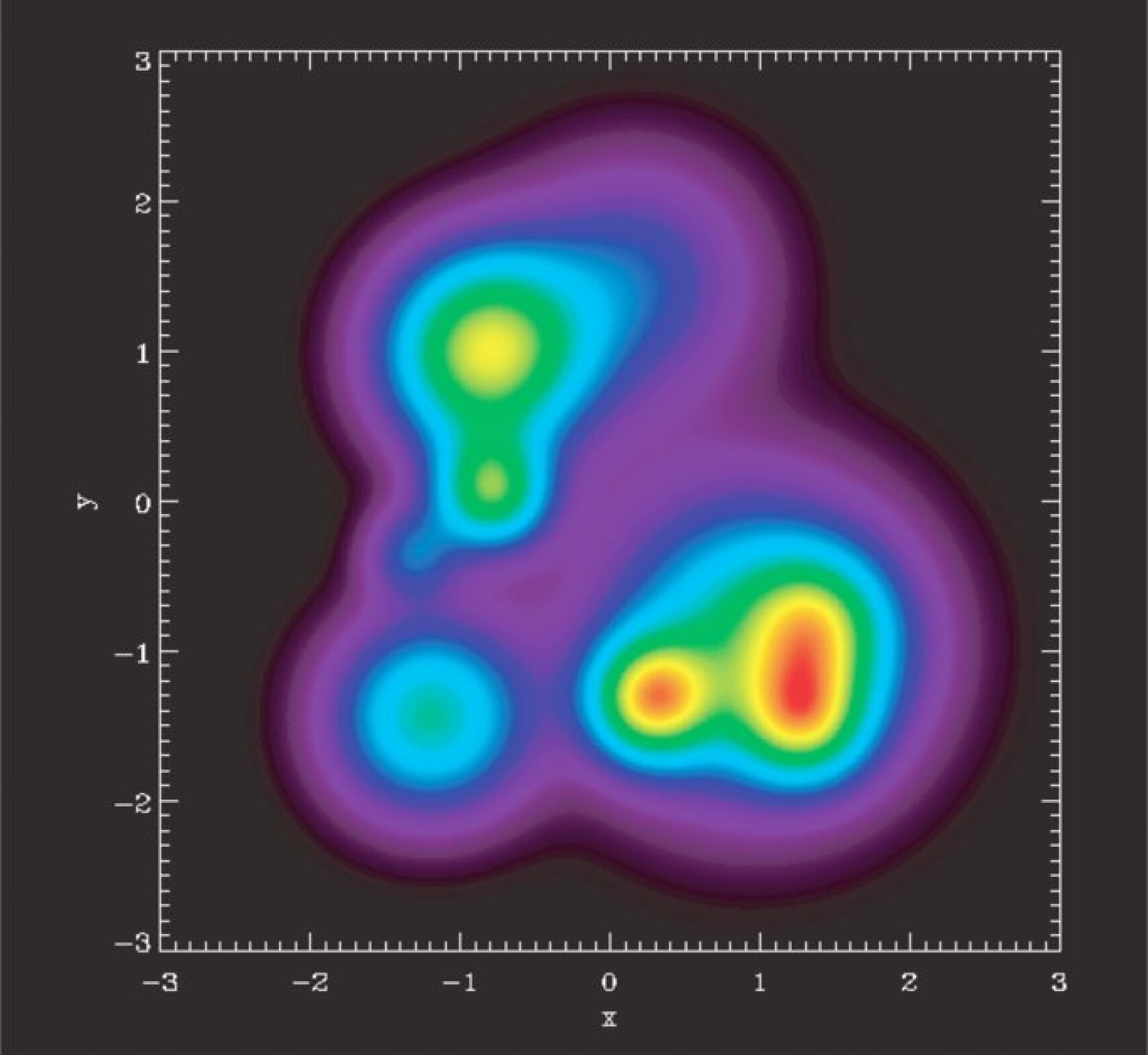
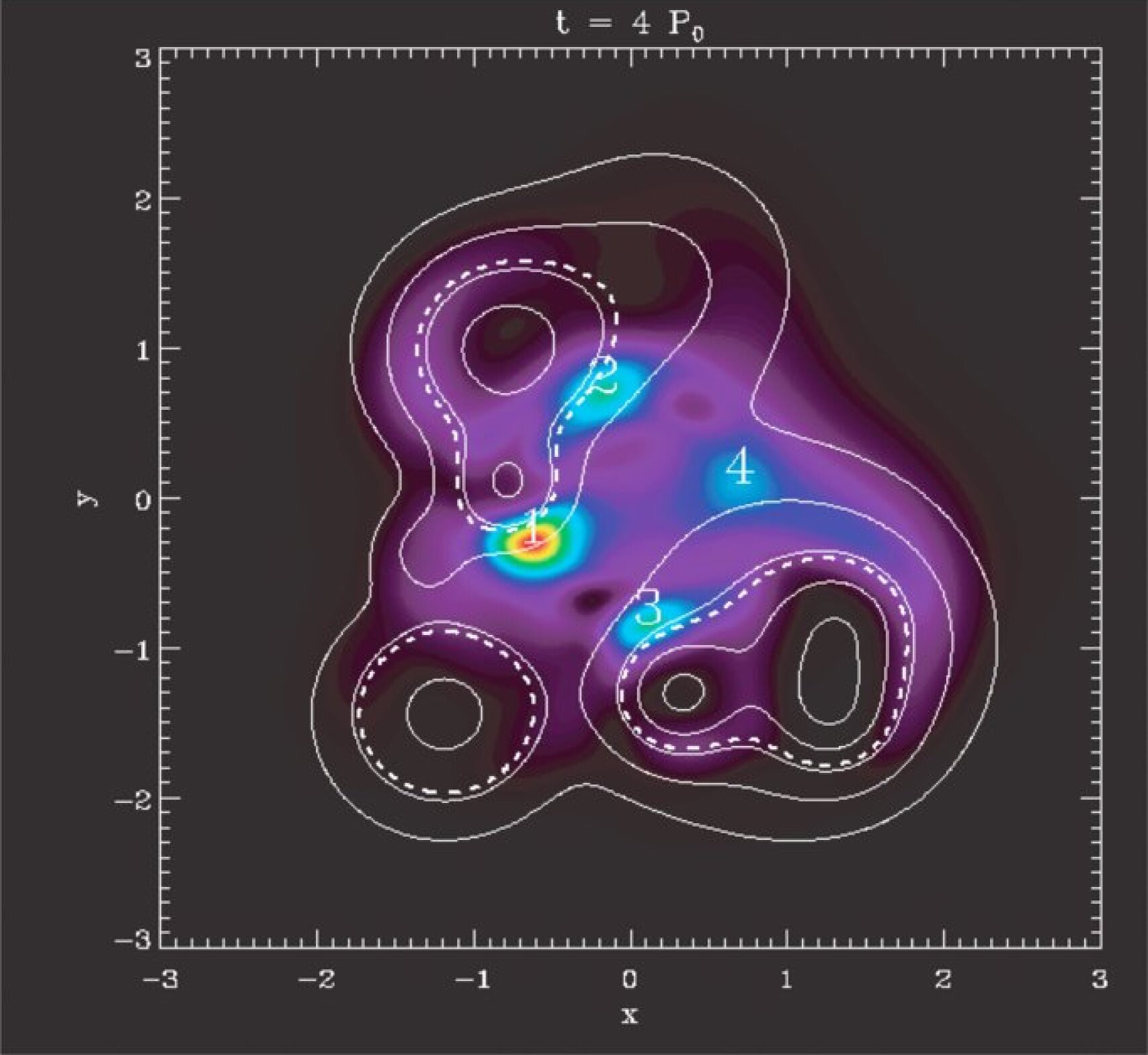
Figure 6: An example of resonant absorption in an inhomogenous corona. The left panel shows the contours of density in a cross-section perpendicular to the magnetic field. The largest density is a factor of 2 greater than the external plasma. The right panel shows the concentration of wave energy at regions where the local Alfvén speed equals the kink speed of the local density maxima. Figure adapted from Pascoe et al. (2011) with permission of the AAS.

The presence of a continuous Alfvén speed profile showcases the first example of the joint influence of different wave damping mechanisms; in this case, resonant absorption and phase mixing. The resonant Alfvénic waves within the inhomogeneous layer (arising from the transfer of energy from the kink mode) can then propagate along magnetic surfaces at different Alfvén speeds, hence are subject to phase mixing (Terradas et al. 2008; Soler & Terradas 2015). The expression for phase mixing lengths, Eq. 10, has been shown to provide a good description of the development of small-scales in analytical and numerical models of kink mode damping (e.g., Pascoe et al. 2013; Soler & Terradas 2015). This dual process has been demonstrated to be robust in multi-stranded structures (Terradas et al. 2008) and with arbitrary inhomogeneities (Pascoe et al. 2011). Figure 6 shows numerical results from Pascoe et al. (2011), where a collection of over-dense magnetised plasma structures were driven as to excite the kink mode. After some time in the simulation, the wave energy of the global mode can be seen to be concentrated towards the boundaries of the structures (Figure 6 right panel), with concentrations close to the locations where $\omega_{A}({x},y)=\omega_{k}$. The details of the dual process are similar at a plasma interface (Lee & Roberts 1986; Hollweg & Yang 1988), which is not so surprising given the fact that the kink mode can be described as a surface Alfvén wave. This would suggest that resonant absorption and phase mixing are key features of Alfvénic wave damping throughout the solar atmosphere, even if coronal structures are collections of magnetic fields associated with diffuse and complex density structures (as suggested by, e.g., Magyar & Van Doorsselaere 2016; Malanushenko et al. 2022).

In terms of contributing to the coronal heating it appears that the actual heating rates, due to the combination of the resonant absorption of kink modes and subsequent phase mixing of rotational motions, are inadequate to compensate for the radiative losses (Pagano & Moortel 2017; Howson et al. 2020), even when a realistic broadband driver is employed (Pagano & De Moortel 2019; Pagano et al. 2020). Further, observational estimates of the frequency-dependent damping rate of propagating kink waves in the quiet Sun suggest that resonant wave damping is likely small (Tiwari et al. 2021; Morton et al. 2021). In coronal holes the Alfvénic waves are found to largely undamped (e.g., Dolla & Solomon 2008; Banerjee et al. 2009; Morton et al. 2015). This pattern of weak damping and no damping could reflect that the density differences across the inhomogeneities are small in the quiet Sun and smaller in coronal holes. Further, it would appear that the transfer of energy to the rotational modes is small and any subsequent phase mixing is also weak.

We note that there has been some evidence for wave damping in coronal holes above 1.2 $R_{\odot}$ (Bemporad & Abbo 2012; Hahn et al. 2012; Hara 2019), inferred from a decrease in the non-thermal widths of spectral lines (which is often taken as an indicator of Alfvénic waves). The suggested rapid damping is somewhat surprising and there is difficulty in explaining it through known wave damping mechanisms. The results have only been found in Hinode EIS data so far, with the suggestion that uncertainties in scattered light may account for the observed decrease in line widths (Zhu et al. 2021). Further, Gilly & Cranmer (2020) suggest that failure to take into account non-equilibrium ionisation and line broadening from the solar wind can lead to misleading inferences from spectral line widths. There have also been other suggestions for the observed decrease in line width (see, e.g., Cranmer 2018).

While the situation does not appear to be favourable for wave heating via phase mixing, the effects pertinent to the stability of the resonance layer can influence energy transfer to small scales.

4.2 Instabilities

The role of wave-driven instabilities has received significant focus in the last few years and appears to be an important ingredient for effective wave energy dissipation in the solar atmosphere. The instabilities are localised processes that are entangled with the dynamics and inhomogeneity of the plasma. While there are many instabilities that can occur in a plasma, there has been a particular focus on the Kelvin-Helmholtz (KH) instability in conjunction with propagating Alfvénic waves in a cylindrical waveguide.

The KH instability is a fluid instability formed by two fluids undergoing differential shearing motion across an interface, with the instability destroying the shear layer through the development of vortices. The KH instability can also occur in magnetized plasma if the velocity is perpendicular to the magnetic field, although its properties are modified by the magnetic field due to the frozen-in condition. However, for a velocity shear parallel to the magnetic field, the instability cannot develop as the magnetic tension has a stabilizing effect (Chandrasekhar et al. 1961). If the magnetic field is sheared across the instability, this can have a stabilizing or destabilizing effect on the KH mode, depending on the properties of magnetic shear (Ofman et al. 1991). KH has been studied theoretically in the context of coronal plasmas, where it is believed to play an important role in the transition to turbulence and heating (e.g., Heyvaerts & Priest 1983; Ofman et al. 1994; Karpen et al. 1994).

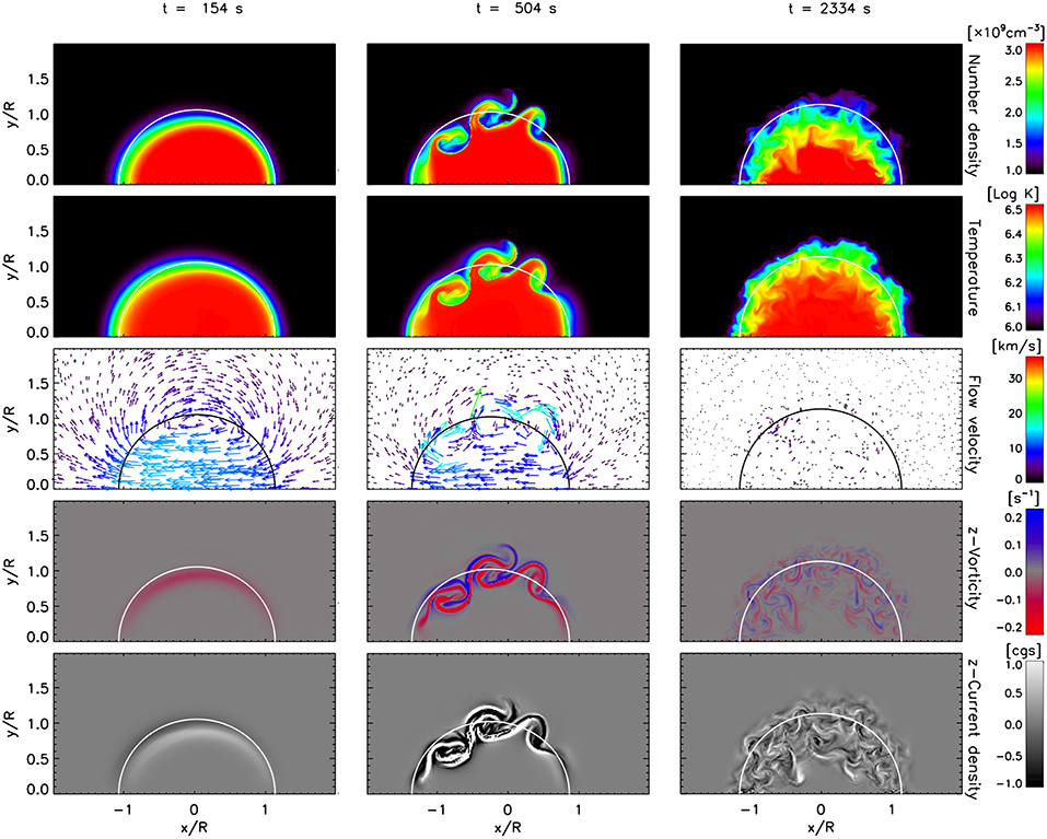
Figure 7: Development of the Kelvin Helmholtz instability at the boundary of a magnetised plasma cylinder. In descending order, the rows show the number density, temperature, flow velocity vectors, parallel vorticity and parallel current. Towards the end of the simulation, the small-scales present are much better observed in the parallel vorticity and current. Reproduced from Antolin & Van Doorsselaere (2019).

With respect to wave motions, it was suggested that because Alfvén waves can oscillate on neighbouring magnetic surfaces without interacting, hence can have an arbitrary phase with respect to each other. This would result in shear flows between the surfaces, which could be susceptible to the KH instability. The instability can then enhance the efficiency of the wave dissipation by more rapidly generating small-scales than phase mixing alone (Heyvaerts & Priest 1983; Hollweg 1984; Hollweg & Yang 1988). The development of the KH instability was shown to be present in numerical non-linear studies of the resonant absorption of Alfvén waves in inhomogeneous plasma (e.g., Ofman et al. 1994; Karpen et al. 1994).

More recently, the development of KH was also shown to be present at the boundary of cylindrical flux tubes undergoing kink motions (an example of this is shown in Figure 7, but see also, e.g., Terradas et al. 2008; Soler et al. 2010; Antolin et al. 2014; Magyar & Van Doorsselaere 2016; Antolin et al. 2017; Karampelas et al. 2019). The transverse motions of the flux tube through an ambient plasma naturally leads to a shear layer at the tube boundary, which is at an angle to the magnetic field (see the flow velocity in Figure 7). Soler et al. (2010) demonstrated that for a non-twisted cylindrical flux tube with a discrete change in density at the boundary, the dispersion relation (in the thin tube approximation) is given by

$$\omega\approx\frac{\rho_{i}}{\rho_{i}+\rho_{e}}m\delta v\pm\left[\frac{(\rho_{i}v^{2}_{Ai}+\rho_{e}v^{2}_{Ae})}{(\rho_{i}+\rho_{e})}k^{2}_{z}-\frac{\rho_{i}\rho_{e}}{(\rho_{i}+\rho_{e})^{2}}m^{2}\delta v^{2}\right]^{1/2},$$ (12)

where $\delta v$ is the velocity jump at the shear layer. In the absence of magnetic twist, the shear flow is perpendicular to the magnetic field. The two terms within the square brackets represent the suppression term (which is essentially the square of the kink speed) and the driving term, respectively. The stability of the shear layer depends upon relative sizes of these two terms. A similar term can be obtained for surface Alfvén waves (Hillier et al. 2018).

As discussed, the resonant conversion of the kink mode to local Alfvén modes in the inhomogeneous layer also leads to phase mixing and further increases the shear velocity (Antolin et al. 2014; Antolin & Van Doorsselaere 2019). The KH instability is found to develop more slowly in the presence of an inhomogeneous layer (Terradas et al. 2008). It appears the reason for this is not yet clear (P. Antolin, private communication), but simulations show that the onset times are longer for increasing inhomogeneity length-scales. Antolin & Van Doorsselaere (2019) suggest this is due to the fact that the larger inhomogeneous length scales preferentially excite unstable modes with larger wavelengths, which have slower growth rates. Further, the KH instability distorts the inhomogeneous layer, thereby widening it and enabling the Alfvénic motions to become present in a greater portion of the loop (Antolin et al. 2014). This process could be severe, and result in complete distortion of an initial circular cross-section (as discussed in Section 1.3 Magyar & Van Doorsselaere 2016). The development of the KH instability can be delayed by the presence of magnetic twist (Soler et al. 2010; Terradas et al. 2018) or large values of dissipative coefficients (Howson et al. 2017), but the boundary of the oscillating loop is always unstable (Barbulescu et al. 2019).

The presence of the KH instability is also prominent when a cylindrical flux tube is perturbed as to only excite torsional Alfvén modes (Guo et al. 2019; Díaz-Suárez & Soler 2021). The development of the instability occurs in much the same manner as the kink mode, suggesting the initial shear from the swaying motion of the kink mode is not a necessary condition to generate the instability in the wave guide. For the KH instability from torsional modes, it is the phase mixing of the Alfvén waves that leads to the velocity shears, as suggested by Heyvaerts & Priest (1983). Díaz-Suárez & Soler (2021) undertook a parameter study showing how the onset of the KH instability is influenced by a number of factors, highlighting the size of the inhomogeneous layer across the flux tube and the density contrast can play key roles. Here, the authors suggest the onset of KH instability is delayed for wider inhomogeneous layers as the phase mixing takes longer to develop and, hence, so does the build-up of shear velocities. For density contrast, the development of the instability occurs faster when the density contrast is larger (although after a certain value, the rate of phase mixing is insensitive to the density contrast).

The development of the KH instability appears to be able to provide a substantial heating of the plasma (Karampelas et al. 2017), unlike the case of resonant absorption and phase mixing. The KH instability can increase the rate at which small-scales are developed from phase mixing alone, hence expediting the transfer of energy to dissipative scales. The development of the KH instability and subsequent heating can be increased when multiple modes are initially present (Guo et al. 2019). It was shown by Shi et al. (2021) that the development of KH instability in simulations of kink oscillations can provide heating rates, that under specific conditions are sufficient enough to balance radiative losses in the quiet Sun.

It should be noted that the majority of these studies focus on standing kink modes, which have, to date, only been identified in active regions. In contrast, observations of Alfvénic waves in the quiet Sun and coronal holes appear to show only propagating modes (Morton et al. 2015; Tiwari et al. 2021; Morton et al. 2021). It would appear that the KH instability is also able to develop in numerical simulations of a system containing only propagating Alfvénic waves, although the low resolution of the simulations prevented detailed study of the instability (Pagano & De Moortel 2019). However, Zaqarashvili et al. (2015) suggest propagating waves are stable to the KH instability as the magnetic and velocity perturbations of Alfvénic modes are in anti-phase, meaning that that magnetic field stabilises the system. Hence, there is still some ambiguity around what conditions are required for the KH instability to develop in a system primarily containing propagating waves.

4.3 Turbulence

Turbulent cascades have long been considered a promising candidate for dissipation of Alfvén waves to heat coronal loops (e.g., Hollweg 1983; Rappazzo et al. 2007; van Ballegooijen et al. 2011; Verdini et al. 2012) and accelerate the solar wind (e.g., Hollweg 1986; Velli et al. 1989; Verdini et al. 2010). Inhomogeneity is essential in many models of Alfvénic wave propagation from the corona to the solar wind. However, it is predominately assumed to be along the field only. More recently the influence of perpendicular inhomogeneity has become of interest. So, to set the scene for this contemporary take, we briefly discuss salient aspects of the long-studied Alfvén wave turbulence (the work in this area is extensive and spans many decades, and an excellent review can be found in Bruno & Carbone 2005).

The incompressible MHD equations that describe the evolution of the magnetic field and the velocity fluctuations can be written in terms of the so-called Elsässer variables, $\vec{z}^{~{}\pm}=\vec{v}\mp\vec{v_{A}}$ (Elsasser 1950), where $\vec{v_{a}}=\vec{B}/\sqrt{\mu_{0}\rho}$. It can be shown that they can be reduced to the following equation:

$$\frac{\partial\vec{z}^{~{}\pm}}{\partial t}+(\vec{z}^{~{}\mp}\cdot\nabla)\vec{z}^{~{}\pm}=-\frac{1}{\rho}\nabla P-\vec{v_{A}}(\nabla\cdot\vec{v_{A}}),$$ (13)

where $P=p+\frac{B^{2}}{2\mu_{0}}$ is the total pressure. The second term on the left hand side describes the non-linear interaction of counter propagating waves along the mean magnetic field, and is the key factor in enabling a turbulent cascade. The non-linear interaction deforms the counter-propagating wave packets and generates the small-scale structures. A typical assumption for Alfvénic turbulence in the corona and solar wind is that there is strong mean magnetic field, such that the amplitudes of perturbations are small in comparison to the background magnetic field (Strauss 1976, referred to as Reduced MHD). With such a strong anisotropy, the cascade is primarily in the perpendicular wavenumbers with parallel cascades suppressed, compared to, e.g., a case with a weaker background field (Oughton et al. 2003).

Typically, the inhomogeneity is only assumed to be along the magnetic field (due to gravitational stratification), and the Alfvénic waves are subject to non-WKB reflection due to the gradient in the Alfvén speed (Heinemann & Olbert 1980; Velli 1993). In the presence of density inhomogeneities along the magnetic field, the final term on the right-hand side of Eq. 13 leads to the reflection of Alfvén waves(Heinemann & Olbert 1980; Velli 1993). This term is vital for the development of turbulence in the solar wind, given it is expected that Alfvénic waves are launched predominantly at the Sun. Without this reflection, there would be no counter-propagating waves to interact. Much of the solar-focused literature on Alfvénic wave turbulence generally only includes this form of reflection to drive the turbulence, with some compressible simulation also able to include Alfvén wave reflection to due to parametric decay instability (e.g., Sagdeev & Galeev 1969; Goldstein 1978; Shoda et al. 2018b, a; Réville et al. 2018).

A compelling development in the discussion of Alfvénic wave turbulence is recent work that has included the presence of perpendicular density inhomogeneities across the magnetic field. Largely this has been neglected in turbulence studies. However, the presence of the inhomogeneity enables a self-cascade of the Alfvénic waves, given the name ‘uni-turbulence’ (Magyar et al. 2017, 2019b). As discussed in Section 2.2, the presence of inhomogeneities perpendicular to the magnetic field leads to the existence of surface Alfvén modes in the presence of a discontinuity, or a quasi/global Alfvénic waves in the presence of a continuous variation (e.g., Goossens et al. 2002, 2012). Magyar et al. (2017) showed via numerical simulations of unidirectional Alfvénic modes that both Elsässer components are present, propagating in the same direction. This leads to the cascade of wave energy in the perpendicular direction, with the timescale for the cascade dependent on the size of the density contrast (Van Doorsselaere et al. 2020a), namely:

$$\tau=\sqrt{5\pi}\frac{1}{\omega a}\frac{\rho_{i}+\rho_{e}}{\rho_{i}-\rho_{e}},$$ (14)

where $a$ is the normalised oscillation amplitude. The presence of both components is due to the fact that, as emphasised already, in inhomogeneous media MHD waves have mixed properties. Magyar et al. (2019a) demonstrate that when compressibility and inhomogeneity of the plasma are taken into account, the Elsässer formalism cannot be used to separate parallel and anti-parallel propagating waves. In a homogeneous, compressible plasma the slow and fast modes are necessarily described by both components. Hence, waves with mixed properties should also have to be described using both Elsässer components. We refer readers to Magyar et al. (2019b) for a discussion of the subtleties of this phenomena applied to Alfvénic modes.

The study of this turbulence phenomenon and its role in plasma heating is still in its infancy but it would appear to be an exciting avenue to aid in the transfer of wave energy to dissipation scales. Application to the damping of standing kink modes in active regions suggest that it could explain an observed non-linear relationship between wave amplitude and damping times (Goddard & Nakariakov 2016; Van Doorsselaere et al. 2021). This phenomenon could also be a dominant source of energy transfer in open field regions, i.e., coronal holes, where the Alfvénic wave propagation appears pre-dominantly uni-directional (i.e., anti-sunward Morton et al. 2015). For closed, loop-like magnetic fields, observations suggest that counter-propagating waves are the norm (Tiwari et al. 2021). These waves are likely driven at both foot-points of the loops (by granulation or mode conversion) and suffer strong wave reflection at the transition region; ensuring a constant supply of counter-propagating waves. Hence, uni-turbulence would play a complementary role. However, Morton et al. (2021) examined a number of loops in the quiescent corona and inferred that the density difference across the inhomogeneities must be small to explain the apparently weak frequency-dependent wave damping of the observed kink modes (i.e., due to resonant absorption). This would also imply that time-scales for energy transfer by uni-turbulence may also be long given Eq. 14.

5 Waves in the chromosphere

In order to reach the corona, the waves originating in the photosphere, must pass through the gauntlet of the chromosphere. This layer remains one of the least understood regions of the Sun’s atmosphere due to many complex physical phenomena that arise there. However, there is a general agreement that the chromosphere is highly dynamic and continuously exchanging mass and energy with the corona (for reviews see, e.g., Judge 2006; Carlsson et al. 2019). Moreover, this complex region is populated by fine-scale structures (see review by Tsiropoula et al. 2012), that bridge the photosphere with the corona and act as conduits for plasma and wave energy transfer across the transition region. A peculiar aspect of this layer is associated with moderate rise in its thermal profile (Fig. 2), as compared to the photosphere. This maintains temperatures of the order of $\sim$10⁴ K in the chromosphere, which enables much of the hydrogen and helium to remain neutral up until the transition region (Figure 8). In these conditions, partial ionisation of plasma becomes a critical factor that can have a strong effect on the dynamics (see reviews by, e.g., Leake et al. 2014; Martínez-Sykora et al. 2015). In combination with large gradients along the magnetic field, it indicates that most of the non-thermal energy remains in the chromosphere.

The observed dynamics of chromospheric features reflect the presence of confined MHD waves that emanate from the photosphere. Alfvénic waves are routinely observed and are often classified as a particular wave mode depending upon their observational characteristics (see review by Verth & Jess 2016). They carry mass, energy and momentum across this layer. However, in the lower solar atmosphere there are two major factors that influence Alfvénic wave propagation, Namely the presence of partial ionisation (which leads to wave damping) and the gradient of the Alfvén speed (Fig. 3, leading to reflection and non-linear effects).

5.1 Partial ionisation

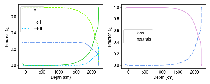
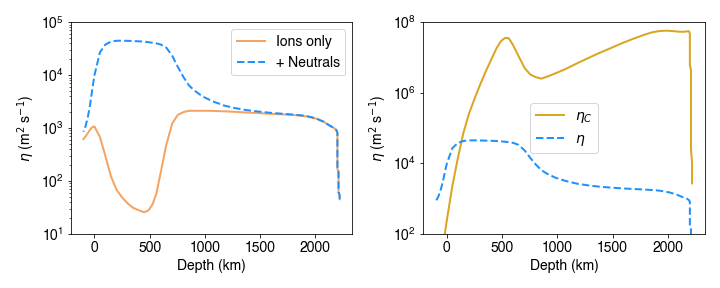
Figure 8: Properties of the partially ionised solar atmosphere based on the FAL-C atmosphere. The top left panel displays the relative fraction of different components of the plasma. The top right plasma composition in terms of the relative fractions of ions and neutrals fractions. The bottom row shows the resistivity through the lower solar atmosphere. The left panel displays the classical electrical resistivity (i.e., electron collisions). The right panel shows the values of resistivity for electrical (including neutrals) in blue dash and Cowling resistivity in solid orange.

The process of ionisation primarily depends on the (inelastic) collisions between the different constituent particles of the plasma. In Figure 8, we illustrate the ionisation degree for the dominant components required for a multi-fluid solar plasma (i.e., hydrogen and helium), along with the fractions of ions and neutrals. The main influence that partial ionisation has on wave propagation arises through the generalised Ohm’s Law, namely;

$$\frac{\partial\vec{B}}{\partial t}=-\nabla\times(-\vec{v}\times\vec{B}+\eta j_{\parallel}+\eta_{p}j_{\perp}+\frac{1}{en_{e}}\vec{j}\times\vec{B})$$ (15)

where, $j_{\parallel}$ and $j_{\perp}$ are the parallel and perpendicular current respectively. All other symbols have the usual meaning. The second term on the right is the Joule heating (with $\eta$ the electrical resistivity) that describes the electron collisions with ions and neutrals. The third term is due to the additional collisions of ions and neutrals (and $\eta_{p}$ is the Pedersen resistivity), while the fourth term is the Hall term. The Pedersen resistivity can be decomposed into the perpendicular components of the electrical resistivity and the Cowling resistivity , i.e. $\eta_{p}=\eta+\eta_{C}$. The Cowling resistivity for a Hydrogen-Helium plasma is given by (e.g. Zaqarashvili et al. 2013),

$$\eta_{C}=\frac{B^{2}}{\mu_{0}}\frac{\alpha_{He}\xi_{H}^{2}+\alpha_{H}\xi_{He}^{2}+\alpha_{HeH}(\xi_{H}+\xi_{He})^{2}}{(\alpha_{H}\alpha_{He}+\alpha_{H}\alpha_{HeH}+\alpha_{He}\alpha_{HeH})},$$

where, $\xi_{n}$ is the fraction of species $n$, and $\alpha_{n_{1}n_{2}}$ is the coefficient of friction between different species $n_{1}$ and $n_{2}$ (note that a subscript of a single species means the sum of coefficients for ion-neutral collisions associated with the given species).

Studies to evaluate the impact of ion-neutral effects in the solar atmosphere were pioneered by Piddington (1956) and Osterbrock (1961), where these authors first highlighted their importance as a wave damping mechanisms in the chromosphere. Decades later, their initial research was further extended for the analysis of Alfvén wave propagation in a partially ionised single-fluid (i.e., hydrogen) MHD model (De Pontieu & Haerendel 1998; Leake et al. 2005), incorporating more realistic estimates for plasma parameters. It was suggested that wave damping due to Ohmic diffusion is dominant over ion-neutral damping in low photosphere and chromosphere, but can be neglected due to the long damping lengths. However, in the upper chromosphere, the damping is sensitive to ion-neutral effects (which can be inferred the magnitude of the Cowling resistivity in Figure 8) and is effective for high-frequency waves ($f>0.01$ Hz). However, low frequency waves remain unaffected by the presence of neutrals and experience no damping due to this mechanism. Further, Leake et al. (2005) also demonstrated that increasing the magnetic field strength can weaken the damping of waves due to ion-neutral effects. Further, weak damping of Alfvénic waves in partially ionised atmosphere can also create drag forces that can lift the cold/dense plasma against the gravity and generate spicule-like structures in the vertical direction (Haerendel 1992; De Pontieu & Haerendel 1998; James et al. 2003).

Naturally, one should also expect to have additional viscosity effects due to ion-neutral interactions, arising through the momentum equation. Khodachenko et al. (2004) provided a quantitative comparison of the relative magnitudes of damping due to viscous and collisional terms, based on the analytic expressions for the wave damping times. It was demonstrated that ion-neutral effects are more efficient compared to viscous forces for Alfvén waves. Soler et al. (2015b) extended this line of work by incorporating multiple potential damping mechanisms into an analytic investigation, and confirmed that viscosity plays no important role in wave damping throughout the chromosphere. Using a single fluid description, Soler et al. (2015b) included the effects of partial ionisation involving both neutral hydrogen and helium. For Alfvén waves, they showed that Ohmic diffusion dominated the damping at low heights, while ambipolar diffusion became more important at greater heights in the chromosphere. This result was in qualitative agreement with De Pontieu & Haerendel (1998) and Leake et al. (2005), although Soler et al. (2015b) suggested that Ohmic diffusion is actually an important damping mechanism in the low chromosphere (see also Goodman 2011; Tu & Song 2013; Arber et al. 2016). The cause of this difference is mainly due to taking into account the role of electron-neutral collisions when calculating the Ohmic resistivity, which leads to a significant increase in the magnitude of the coefficient (bottom left panel, Figure 8). Soler et al. (2015b) also highlighted the role of the magnetic field strength, which determines at which heights ambipolar damping overtakes Ohmic damping.

Although insightful, the use of single fluid approximations to understand the wave behaviour in the photosphere and chromosphere has been shown to be incorrect. This aspect was examined in detail by Zaqarashvili et al. (2011b), who investigated MHD wave propagation in a two fluid model consisting of neutral hydrogen and ions. They showed that for time-scales less than the ion-neutral collision time, both fluid species tend to behave independently and a single-fluid approximation does not remain valid any more. Importantly, the damping of high frequency waves is a lot weaker than suggested by the single fluid approach. Their results again confirmed that low-frequency waves were not strongly influenced by partial ionisation of the plasma. More generally, Soler et al. (2013) showed that the damping of waves is most efficient when the wave frequency is comparable to the ion-neutral frequency.

Given the sizable fraction of neutral helium in the lower solar atmosphere, Zaqarashvili et al. (2011a, 2013), extended the analysis with the inclusion of three fluids. The addition of helium species was found to have an additional impact on the damping of high frequency Alfvén waves. However, this mechanism is strongly dependent on the plasma temperature, with larger wave damping rates at higher temperatures ($1-4\times 10^{4}$ K), when ionisation of hydrogen becomes prevalent (see Figure 8). Further, Soler et al. (2015a) found that there exists a particular wavelength range for which Alfvén waves are overdamped (10$\lesssim\lambda\lesssim$1000 m), resulting in localised energy dissipation and thus restricting the propagation as Alfvén wave.

In an effort to incorporate perpendicular inhomogenities into studies of wave propagation in a partially ionised plasma, Soler et al. (2012) investigate the influence of ion-neutral collisions on kink wave propagation in a cylindrical flux tube in a two-fluid study. The influence of the ion-neutral interaction was incorporated in the momentum equation through frictional terms. With this formalism, Soler et al. (2012) found that ion-neutral collisions appear to have little impact on kink wave propagation and resonant absorption remained the dominant damping mechanism. Interestingly, they found that the damping lengths due to resonant absorption, for kink waves with periods less than 10 s, are smaller than or of the same order as the height of the chromosphere. Hence, they suggested that only waves with periods greater than 10 s are able to reach the coronal level in the form of kink motions, while the shorter period waves would reach the corona as rotational motions.

Finally, we note that use of the multi-fluid approach has been suggested to be invalid for short wavelengths. This was first highlighted by Soler et al. (2015a) who demonstrated that the multi-fluid approach, which essentially treats each plasma species separately, is not applicable to high-frequency waves below of heights $\sim 900$ km. They suggest a kinetic description of the plasma is required as both ions and electrons collide too frequently with the neutrals, meaning that the thermal properties of each species are not independent.

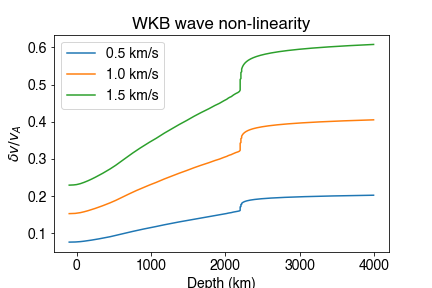
Figure 9: The ratio of wave velocity amplitude to Alfvén speed is shown as a function of height. The curves are calculated using a WKB approximation for wave amplification in an ideal plasma using the density from the FAL model and the magnetic field from the empirical model, see Figure 2.

5.2 Alfven speed gradient

Aside from the longitudinal homogeneity in ionisation state, there is also a longitudinal inhomogeneity in the Alfvén speed through the chromosphere due to the decrease in density (Figure 2). This variation leads to amplification of the waves propagating from the photosphere to the corona. The relationship between wave amplitude and density can be obtained under a WKB approximation, namely $\mid\delta v\mid\propto\rho^{-1/4}$. Hence, the upwardly propagating Aflvén waves can become non-linear, demonstrated by the increase of the ratio of the wave amplitude to the Alfvén speed ($\mid\delta v\mid/v_{A}$) with height (shown in Figure 9). Given that the profiles in Figure 9 are found using the WKB approximation, they are not valid for waves with wavelengths comparable to or greater than the density scale height in the lower solar atmosphere. Moreover, the calculation of the profiles neglects any physics that would act to damp these waves, e.g. ion-neutral effects, Ohmic diffusivity, and mode conversion (of which we now discuss). Hence, in reality the increase in wave amplitude is less rapid than shown in the figure.

The large amplitude of the Alfvén waves leads to an increase in the ponderomotive force, which is able drive motions parallel to the magnetic field. This enables the mode conversion of Alfvénic modes to both fast and slow magnetoacoustic modes (e.g., Hollweg et al. 1982; Hollweg 1992). Both the fast and slow waves also develop into shocks in the upper chromosphere and low corona. When the magneto-acoustic shock occurs in the chromosphere, there is an upward displacement of the chromosphere and transition region creating spicule-like structures (e.g., Hollweg et al. 1982; Hollweg 1992). The slow shocks driven by Alvén waves are found to be very effective at heating the lower solar atmosphere (Matsumoto & Suzuki 2012; Arber et al. 2016; Wang & Yokoyama 2020). Arber et al. (2016) suggest that the relative heating rates due to shock heating are four orders of magnitude greater than the Pederson resistivity. However, the heating rate in their 1.5D simulations may be enhanced by shock coalescence. The fast and slow mode waves produced by Alfvén waves are also capable of heating the corona (Hollweg 1992; Kudoh & Shibata 1999; Moriyasu et al. 2004; Antolin et al. 2008; Antolin & Shibata 2010).

The variation in Alfvén speed also leads to significant reflection of the waves in the chromosphere, and especially at the transition region. The reflection of waves occurs if the wavelength of the wave is comparable or greater than the length-scale over which there is appreciable variation in Alfvén speed (e.g., Ferraro & Plumpton 1958; Velli 1993). Hence there is frequency filtering effect, with low frequency Alfvén waves affected to a greater extent than higher frequency waves (see Figure 10 panel c for a curve of reflection versus frequency; details of calculation given in Soler et al. 2017, 2019). The wave reflection also sets up a system of counter propagating waves in the chromosphere, which, as discussed in Section 4.3, enables Alfvénic wave turbulence to develop (e.g., van Ballegooijen et al. 2011).

In general, the transition region provides a substantial barrier to all waves, significantly influencing the transmission to the corona (Hollweg 1981; Verdini et al. 2012), with Cranmer & van Ballegooijen (2005) suggesting the reflection rate is on the order of 95%. Fully dynamical simulations suggest the wave reflection might be lower, but still substantial, with 85% of the initial wave energy flux reaching the corona (Suzuki & Inutsuka 2005; Suzuki & ichiro Inutsuka 2006). In the Suzuki & Inutsuka (2005); Suzuki & ichiro Inutsuka (2006) model, the transition region is dynamic due to intermittent shock heating in the chromosphere and the sharp density gradient is smoothed out. Arber et al. (2016) estimate of the efficiency of wave transmission to the corona by comparing the Poynting flux at the photosphere against the Poynting flux entering the corona. In their incompressible simulation, the transmission to the corona is a relatively smooth function of frequency. The transmission is most effective for intermediate frequencies, peaking at around 40% of the initial wave flux for frequencies of 0.1-1 Hz, with the reduction in transmission for higher frequencies related to wave damping. The degree of magnetic expansion can also influence the transmission curve, with larger rates of expansion shifting the transmission peak to lower frequencies (Similon & Zargham 1992; Soler et al. 2017). In Figure 10 we show the reflection, transmission (to corona) and absorption (i.e., dissipation due to wave damping) curves for a model of Alfvén wave propagation from Soler et al. (2019) model (which show a qualitatively similar behaviour to that in Arber et al. 2016).

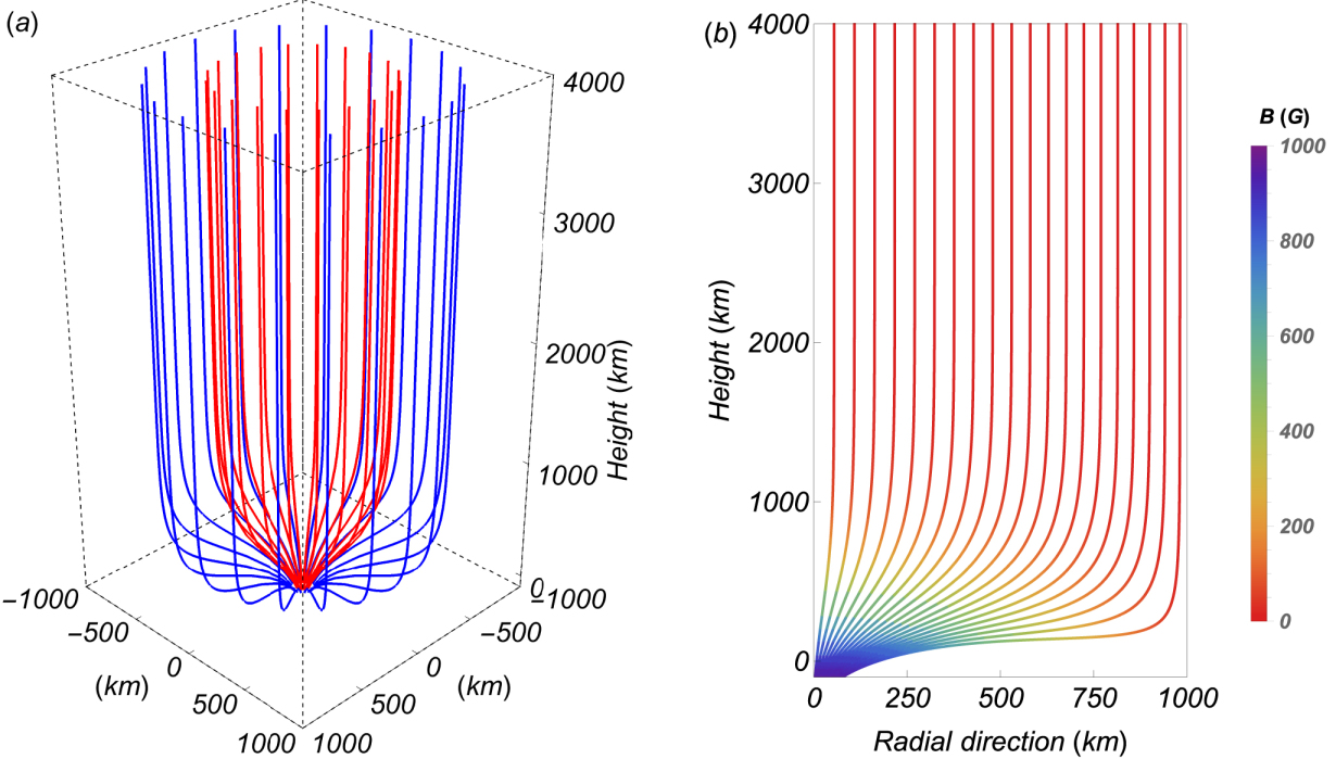
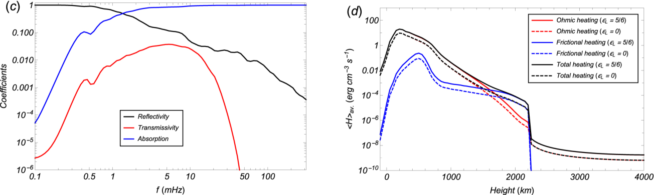
Figure 10: The structure of the magnetic field from the model of torsional Alfvén wave propagation through the lower solar atmosphere from Soler et al. (2019). Panel a shows the expanding magnetic field in 3D. Panel b displays a cross-sectional profile of the magnetic field in the radial direction. Panel c is the horizontally averaged profiles for reflection, transmission and absorption as a function of wave frequency. Panel d shows the contribution to the wave heating rates as a function of height in the model atmosphere. Figures reproduced from Soler et al. (2019) with permission of the AAS.

5.3 Perpendicular inhomogeneity

From the previous discussions, it is clear that Alfvénic wave propagation is strongly influenced by the perpendicular inhomogeniety of plasma, hence it is worth touching upon its influence in a partially ionised plasma. While there are a number of 2D and 3D models of wave propagation through the lower atmosphere that include or develop some perpendicular inhomogeniety (e.g., Shelyag et al. 2016; Kuźma et al. 2020; Battaglia et al. 2021; Breu et al. 2022), a fascinating insight can be found in Soler et al. (2019). The model focuses on the propagation of torsional Alfvén modes from photosphere to corona but is quite restrictive; it is an incompressible, 2.5D model of linear waves. However, it is an insightful culmination of a series of works that carefully increases the models complexity and isolates the impact of aspects of wave physics (see Soler et al. 2013, 2015b, 2017, 2019, 2021). In Soler et al. (2019), the perpendicular inhomogeniety arises through the implementation of a 3D magnetic field, which is shown in Figure 10. Through the chromosphere the magnetic field expands but that expansion rate varies as a function of radius. As such, there is a variation of the Alfvén speed in the perpendicular direction, as well as the parallel direction. This leads to phase mixing of the Alfvén waves and the development of small-scale shears in the velocity and magnetic perturbations across the flux tube. In turn, this leads to an enhancement of local currents and increases the rate of Ohmic diffusion.

Some of key results from the Soler et al. (2019) are shown in Figure 10, which also nicely summarises aspects of the previous discussions. In panel c, the reflection, transmission and absorption (i.e. wave damping) of the waves are shown as a function of frequency. There is clear frequency dependency for all quantities. It can be immediately seen that the transmission of wave energy to the corona is drastically reduced compared to the estimates from the lower dimensional models discussed previously. The peak of the transmission curve is close to 5 mHz, and only $\sim$1% of the photospheric wave energy flux is able to reach the corona. The reason for the decrease in transmission is due to the increase in Ohmic heating arising from the phase mixing. Ohmic heating now dominates the frictional heating (due to ion-neutral collisions) through the majority of the lower atmosphere (panel d), and it is only surpassed in the upper chromosphere ($\sim 1700$ km). In this model, the Ohmic heating rate has increased while the frictional heating rate is similar to previous lower dimensional models (Soler et al. 2017). For an injected wave flux at the photosphere with a realistic total energy of $~{}10^{9}$  erg cm^-2 s^-1, the wave flux entering the corona turns out to be only a factor of two smaller than the expected energy flux required to sustain coronal temperatures in the quiet Sun.

We note that the sensitivity of this result to the magnetic geometry, namely the height of the most significant expansion, is not entirely clear but could play a role in determining the relative contributions of the two heating mechanisms. Additionally, given the strong influence of shock heating in the 1.5D models of Arber et al. (2016), it remains to be seen if the findings from Soler et al. (2019) are still valid for non-linear wave propagation.

Another interesting work comes from González-Morales et al. (2020), who take a different approach to examining the impact of inhomogeneities on wave propagation. The framework is single fluid 3D MHD but incorporates the generalised Ohm’s Law (Eq. 15) and additional terms in the energy equations to describe a partially ionised plasma. Instead of focusing on a single flux-tube, a small region of the quiet Sun is modelled and includes solar magneto-convection with a near self-generated magnetic field. This naturally generates magnetic flux tubes through the concentration of flux in the intergranular lanes. The model does not reach the corona but is confined to the lower solar atmosphere. The realistic nature of the magneto-convection means that there are gradients perpendicular to the magnetic field direction throughout the simulation domain. The paper does not discuss phase mixing of Alfvén waves or associated instabilities (although they should be present) but does highlight the important role of two other effects, ambipolar diffusion and the Hall term. In common with Soler et al. (2019), González-Morales et al. (2020) find that ion-neutral effects can lead to efficient absorption of Poynting flux. Due to the highly inhomogeneous nature of the plasma, MHD waves and associated instabilities (e.g., Kelvin-Helmholtz) enhance vorticity (e.g., Goossens et al. 2019; Howson et al. 2019), which in turn increases the magnitude of the currents (e.g., Howson et al. 2021) and increasing the Ohmic and ambipolar heating rates. Futhermore, the inclusion of the Hall term is found to result in a doubling of the Poynting flux at the upper chromosphere (compared to without its presence), which is partially due to a Hall-induced mode coupling of fast and Alfvén waves (see also Cally & Khomenko 2015; González-Morales et al. 2019).

6 Summary

The solar atmosphere is a complex plasma environment that is characterised by the networks of magnetic field that thread it, and the large variations in plasma parameters with height. The temperature, density and magnetic field vary by orders of magnitude from the photosphere to the corona and solar wind, and makes the Sun’s atmosphere an interesting laboratory for studying MHD wave propagation. In addition to the large-scale variations, the plasma is also observed to be highly structured on small-scales ($\sim$100’s km) perpendicular to the magnetic field (although there could be much finer structuring below the current limits of instrumentation), likely the result of localised heating events that are believed to take place throughout the atmosphere. As we have hopefully highlighted through the review, the presence of plasma inhomogenities in the solar atmosphere produces a fantastic array of physics that impacts upon wave propagation through the magnetised plasma.

The main motivation for many investigations of Alfvénic waves is to understand their role in the heating of the atmospheric plasma and the acceleration of the solar wind (they are also proving useful for magneto-seismology and estimates of the coronal magnetic field, e.g., Anfinogentov & Nakariakov 2019; Yang et al. 2020). For the waves to contribute to these processes, they need to propagate upwards from the photosphere into, and through, the partially ionised, magnetically-dominated chromosphere. A fraction of the Alfvénic waves are able to cross the barrier provided by the dramatic drop in density at the transition region, reaching the corona and beyond. We have discussed various details of the journey, but typically in isolation. This somewhat reflects how the research has been undertaken to date. As mentioned at the beginning of this review, it is challenging to include all the necessary physics into a single atmospheric model. Hence, to date, many studies have focused on individual problems in isolation in order to make progress (this, of course, is always the way). So to wrap up this review, we highlight a few representative state-of-the-art numerical studies and note the current tensions in the modelling.

There are many large-scale models that examine wave propagation, focusing on, e.g., wave heating/acceleration of the solar wind over 10’s of solar radii, or global simulations of coronal heating. While demonstrating the feasibility of wave-based plasma heating/wind acceleration via turbulence, one of the main sacrifices these models make is that they largely ignore the role of perpendicular inhomogeneity; missing resonances, phase mixing and instabilities. There are also other restrictions required to make these numerical simulations feasible. For example, the latest Alfvén wave solar wind simulations have been able to incorporate compressibility into a 3D system to examine the non-linear coupling to slow modes, but only starting at the coronal base (e.g., Shoda et al. 2019) or includes a simple lower atmosphere with a reduced numerical resolution (Matsumoto 2020). Another examines the propagation of Alfvén waves from the lower atmosphere and the onset of parametric instabilities, but using a 1D single fluid approach ignoring partial ionisation (e.g., Réville et al. 2018). Moreover, a global model of coronal heating based on Alfv́en wave turbulence (the Alfvén wave solar model - AW-SoM, van der Holst et al. 2014) is able to reproduce global EUV emission reasonably well, but only includes wave propagation from the upper chromosphere and uses Reduced MHD and WKB wave propagation (with correction terms) to predict wave heating rates. Also, smaller-scale Alfvénic-wave-driven turbulence models, i.e. focusing on single flux tubes, appear to be able to reproduce necessary heating rates for chromospheric/coronal plasma, but only include a basic photosphere/chromosphere without dynamics or multi-fluid effects (e.g., Matsumoto 2018), and are often based on Reduced MHD (e.g., van Ballegooijen et al. 2011; Verdini et al. 2012).

There are also a wealth of studies, some of which we discussed here, that concentrate on the impact of non-ideal phenomena and instabilities on wave propagation; requiring high-resolution simulations to capture the relevant scales. Hence the models are typically confined to the lower atmosphere or are single, highly idealised flux tubes, with many of the latter models confined to the coronal section or include only a basic lower atmosphere (i.e., no dynamics or partial ionisation). For example, as discussed in Section 5.3, González-Morales et al. (2020) undertook hydrodynamic convection driven 3D simulations of lower atmosphere including a generalised Ohm’s law and examining the impact of ambipolar diffusion and the Hall term on Alfvénic waves. However, the simulation domain was confined to heights below 1.5 Mm. To include a corona, Soler et al. (2019) model a single flux tube with a temporally stationary atmosphere based on the FAL atmosphere, solving linearised multi-fluid wave equations. The linearisation obviously means that shocks, mode conversion and momentum transfer are not present, all of which are representative of the observed chromosphere. Moreover, most models with a multi-fluid chromosphere do not include time-dependent hydrogen ionisation, which acts over relatively long time-scales (e.g., Leenaarts et al. 2007). Hence the chromospheric ionisation fraction and temperature are different from equilibrium which would influence the efficacy of various multi-fluid phenomena, e.g., Cowling resistivity.

The final note to end on is a comment on the observations of Alfvénic waves in the lower solar atmosphere and corona. To date, the observational studies have been relatively few (excluding work on the standing kink modes in active regions), and little is known from an observational perspective. Over the last three decades there have been a number of indirect measurements of their presence through spectral line broadening (e.g., Banerjee et al. 1998, 2009; Hahn et al. 2012) in coronal holes and the quiet Sun corona. It took the advent of high-resolution observations to measure the Alfvénic waves directly (Tomczyk et al. 2007; De Pontieu et al. 2007; Jess et al. 2009; McIntosh et al. 2011; Hillier et al. 2013; Morton et al. 2012), but the number of studies focused on analysing the details of propagating waves is few. Those that have been performed have largely focused on measuring the typical properties (e.g., amplitude, period) in a single region and providing energy estimates of the waves in the structures examined (e.g., coronal loops, spicules). However, the details of excitation, evolution and dissipation are scant. Part of this issue is due to the challenge of connecting the observed dynamics through the different regions of the atmosphere. Some of the issue lies in observing the chromosphere, which is complicated by extended formation heights of the resonance lines (requiring narrow spectral filters to isolate different heights, e.g., Judge & Carlsson 2010) and non-local and non-equilibrium contributions to radiative transfer that make interpreting the measured diagnostics formidable (Leenaarts 2020). For the corona, the task is somewhat simpler and there is a wealth of suitable data from the likes of the Coronal Multi-Channel Polarimeter (Tomczyk et al. 2008) and the Solar Dynamic Observatory (Pesnell et al. 2012). It is unclear why more attention hasn’t been given to analysing the coronal Alfvénic waves present in the data. The measurements are challenging (e.g., Thurgood et al. 2014; Weberg et al. 2018; Tiwari et al. 2021) but opportunities exist to compare the theoretical predictions discussed in preceding sections with observed wave behaviour. It is surely an area worthy of focus in the coming years. More attention may be focused on the observational behaviour of Alfvénic waves in the near future when DKIST (Rimmele et al. 2020; Rast et al. 2021) and Solar Orbiter (Müller et al. 2020) provide images of the chromosphere and corona at unprecedented spatial and temporal resolution. We wait with anticipation to see what wave physics these new facilities might uncover.

References

- Alfvén (1941) Alfvén, H. 1941, Arkiv för Matematik Astronomi och Fysik, 27A, 1
- Andries et al. (2005a) Andries, J., Arregui, I., & Goossens, M. 2005a, ApJ, 624, L57
- Andries et al. (2005b) Andries, J., Goossens, M., Hollweg, J. V., Arregui, I., & Van Doorsselaere, T. 2005b, A&A, 430, 1109
- Andries et al. (2009) Andries, J., van Doorsselaere, T., Roberts, B., et al. 2009, Space Sci. Rev., 149, 3
- Anfinogentov & Nakariakov (2019) Anfinogentov, S. A. & Nakariakov, V. M. 2019, The Astrophysical Journal, 884, L40
- Antolin et al. (2017) Antolin, P., Moortel, I. D., Doorsselaere, T. V., & Yokoyama, T. 2017, The Astrophysical Journal, 836, 219
- Antolin & Shibata (2010) Antolin, P. & Shibata, K. 2010, ApJ, 712, 494
- Antolin et al. (2008) Antolin, P., Shibata, K., Kudoh, T., Shiota, D., & Brooks, D. 2008, The Astrophysical Journal, 688, 669
- Antolin & van der Voort (2012) Antolin, P. & van der Voort, L. R. 2012, The Astrophysical Journal, 745, 152
- Antolin & Van Doorsselaere (2019) Antolin, P. & Van Doorsselaere, T. 2019, Frontiers in Physics, 7, 85
- Antolin et al. (2014) Antolin, P., Yokoyama, T., & Van Doorsselaere, T. 2014, ApJ, 787, L22
- Arber et al. (2016) Arber, T. D., Brady, C. S., & Shelyag, S. 2016, ApJ, 817, 94
- Arregui (2015) Arregui, I. 2015, Philosophical Transactions of the Royal Society A: Mathematical, Physical and Engineering Sciences, 373, 20140261
- Aschwanden et al. (1999) Aschwanden, M. J., Fletcher, L., Schrijver, C. J., & Alexander, D. 1999, ApJ, 520, 880
- Aschwanden et al. (2000) Aschwanden, M. J., Nightingale, R. W., & Alexander, D. 2000, ApJ, 541, 1059
- Aschwanden et al. (2003) Aschwanden, M. J., Nightingale, R. W., Andries, J., Goossens, M., & Doorsselaere, T. V. 2003, The Astrophysical Journal, 598, 1375
- Ballester et al. (2018) Ballester, J. L., Alexeev, I., Collados, M., et al. 2018, Space Science Reviews, 214
- Banerjee et al. (2009) Banerjee, D., Pérez-Suárez, D., & Doyle, J. G. 2009, A&A, 501, L15
- Banerjee et al. (1998) Banerjee, D., Teriaca, L., Doyle, J. G., & Wilhelm, K. 1998, A&A, 339, 208
- Barbulescu et al. (2019) Barbulescu, M., Ruderman, M. S., Doorsselaere, T. V., & Erdélyi, R. 2019, The Astrophysical Journal, 870, 108
- Battaglia et al. (2021) Battaglia, A. F., Canivete Cuissa, J. R., Calvo, F., Bossart, A. A., & Steiner, O. 2021, A&A, 649, A121
- Bel & Leroy (1977) Bel, N. & Leroy, B. 1977, A&A, 55, 239
- Bellot Rubio & Orozco Suárez (2019) Bellot Rubio, L. & Orozco Suárez, D. 2019, Living Reviews in Solar Physics, 16, 1
- Bemporad & Abbo (2012) Bemporad, A. & Abbo, L. 2012, ApJ, 751, 110
- Berger et al. (1998) Berger, T. E., Loefdahl, M. G., Shine, R. S., & Title, A. M. 1998, ApJ, 495, 973
- Berger & Title (1996) Berger, T. E. & Title, A. M. 1996, ApJ, 463, 365
- Bogdan et al. (1993) Bogdan, T. J., Brown, T. M., Lites, B. W., & Thomas, J. H. 1993, The Astrophysical Journal, 406, 723
- Bogdan et al. (2003) Bogdan, T. J., Carlsson, M., Hansteen, V. H., et al. 2003, ApJ, 599, 626
- Bogdan et al. (1996) Bogdan, T. J., Hindman, B. W., Cally, P. S., & Charbonneau, P. 1996, The Astrophysical Journal, 465, 406
- Bonet et al. (2008) Bonet, J. A., Márquez, I., Sánchez Almeida, J., Cabello, I., & Domingo, V. 2008, Astrophyscial Journal Letters, 687, L131
- Breu et al. (2022) Breu, C., Peter, H., Cameron, R., et al. 2022, A&A, 658, A45
- Brooks et al. (2013) Brooks, D. H., Warren, H. P., Ugarte-Urra, I., & Winebarger, A. R. 2013, ApJ, 772, L19
- Bruno & Carbone (2005) Bruno, R. & Carbone, V. 2005, Living Reviews in Solar Physics, 2, 4
- Cally (2000) Cally, P. 2000, Solar Physics, 192, 395
- Cally (2017) Cally, P. S. 2017, MNRAS, 466, 413
- Cally & Bogdan (1997) Cally, P. S. & Bogdan, T. J. 1997, The Astrophysical Journal, 486, L67
- Cally & Goossens (20008) Cally, P. S. & Goossens, M. 20008, Sol. Phys., 251, 251
- Cally & Hansen (2011) Cally, P. S. & Hansen, S. C. 2011, ApJ, 738, 119
- Cally & Khomenko (2015) Cally, P. S. & Khomenko, E. 2015, The Astrophysical Journal, 814, 106
- Cargill (1994) Cargill, P. J. 1994, ApJ, 422, 381
- Carlsson et al. (2019) Carlsson, M., De Pontieu, B., & Hansteen, V. H. 2019, ARA&A, 57, 189
- Chandrasekhar et al. (1961) Chandrasekhar, S., Elbert, D. D., & Lebovitz, N. R. 1961, Proceedings of the Royal Society of London Series A, 264, 155
- Chitta et al. (2012) Chitta, L. P., van Ballegooijen, A. A., Rouppe van der Voort, L., DeLuca, E. E., & Kariyappa, R. 2012, ApJ, 752, 48
- Choudhuri et al. (1993) Choudhuri, A. R., Auffret, H., & Priest, E. R. 1993, Sol. Phys., 143, 49
- Cranmer (2018) Cranmer, S. R. 2018, The Astrophysical Journal, 862, 6
- Cranmer et al. (2017) Cranmer, S. R., Gibson, S. E., & Riley, P. 2017, Space Science Reviews, 212, 1345
- Cranmer & van Ballegooijen (2005) Cranmer, S. R. & van Ballegooijen, A. A. 2005, ApJS, 156, 265
- Crouch & Cally (2003) Crouch, A. & Cally, P. 2003, Solar Physics, 214, 201
- De Pontieu & Haerendel (1998) De Pontieu, B. & Haerendel, G. 1998, A&A, 338, 729
- De Pontieu et al. (2007) De Pontieu, B., McIntosh, S. W., Carlsson, M., et al. 2007, Science, 318, 1574
- De Rosa & Toomre (2004) De Rosa, M. L. & Toomre, J. 2004, ApJ, 616, 1242
- de Wijn et al. (2009) de Wijn, A. G., Stenflo, J. O., Solanki, S. K., & Tsuneta, S. 2009, Space Sci. Rev., 144, 275
- Defouw (1976) Defouw, R. J. 1976, The Astrophysical Journal, 209, 266
- Díaz-Suárez & Soler (2021) Díaz-Suárez, S. & Soler, R. 2021, A&A, 648, A22
- Dolla & Solomon (2008) Dolla, L. & Solomon, J. 2008, A&A, 483, 271
- Edlén (1941) Edlén, B. 1941, Arkiv för Matematik Astronomi och Fysik, 28B, 1
- Edlén (1943) Edlén, B. 1943, ZAp, 22, 30
- Edwin & Roberts (1983) Edwin, P. M. & Roberts, B. 1983, Sol. Phys., 88, 179
- Elsasser (1950) Elsasser, W. M. 1950, Physical Review, 79, 183
- Ferraro & Plumpton (1958) Ferraro, C. A. & Plumpton, C. 1958, The Astrophysical Journal, 127, 459
- Fontenla et al. (1993) Fontenla, J. M., Avrett, E. H., & Loeser, R. 1993, The Astrophysical Journal, 406, 319
- Giagkiozis et al. (2018) Giagkiozis, I., Fedun, V., Scullion, E., Jess, D. B., & Verth, G. 2018, ApJ, 869, 169
- Giagkiozis et al. (2016) Giagkiozis, I., Goossens, M., Verth, G., Fedun, V., & Doorsselaere, T. V. 2016, The Astrophysical Journal, 823, 71
- Gilly & Cranmer (2020) Gilly, C. R. & Cranmer, S. R. 2020, The Astrophysical Journal, 901, 150
- Goddard & Nakariakov (2016) Goddard, C. R. & Nakariakov, V. M. 2016, A&A, 590, L5
- Goldstein (1978) Goldstein, M. L. 1978, The Astrophysical Journal, 219, 700
- González & Rubio (2009) González, M. J. M. & Rubio, L. R. B. 2009, The Astrophysical Journal, 700, 1391
- González-Morales et al. (2019) González-Morales, P. A., Khomenko, E., & Cally, P. S. 2019, The Astrophysical Journal, 870, 94
- González-Morales et al. (2020) González-Morales, P. A., Khomenko, E., Vitas, N., & Collados, M. 2020, A&A, 642, A220
- Goodman (2011) Goodman, M. L. 2011, The Astrophysical Journal, 735, 45
- Goossens (2003) Goossens, M. 2003, An introduction to plasma astrophysics and magnetohydrodynamics, Vol. 294
- Goossens et al. (2005) Goossens, M., Andries, J., & Arregui, I. 2005, Philosophical Transactions of the Royal Society A: Mathematical, Physical and Engineering Sciences, 364, 433
- Goossens et al. (2012) Goossens, M., Andries, J., Soler, R., et al. 2012, ApJ, 753, 111
- Goossens et al. (2002) Goossens, M., de Groof, A., & Andries, J. 2002, in ESA Special Publication, Vol. 505, SOLMAG 2002. Proceedings of the Magnetic Coupling of the Solar Atmosphere Euroconference, ed. H. Sawaya-Lacoste, 137–144
- Goossens et al. (2011) Goossens, M., Erdélyi, R., & Ruderman, M. S. 2011, Space Science Reviews, 158, 289
- Goossens & Poedts (1992) Goossens, M. & Poedts, S. 1992, The Astrophysical Journal, 384, 348
- Goossens et al. (2009) Goossens, M., Terradas, J., Andries, J., Arregui, I., & Ballester, J. L. 2009, A&A, 503, 213
- Goossens et al. (2013) Goossens, M., Van Doorsselaere, T., Soler, R., & Verth, G. 2013, ApJ, 768, 191
- Goossens et al. (2019) Goossens, M. L., Arregui, I., & Van Doorsselaere, T. 2019, Frontiers in Astronomy and Space Sciences, 6, 20
- Gošić et al. (2014) Gošić, M., Bellot Rubio, L. R., Orozco Suárez, D., Katsukawa, Y., & del Toro Iniesta, J. C. 2014, ApJ, 797, 49
- Grotian (1939) Grotian, W. 1939, Die Naturwissenschaften, 27, 214
- Gudiksen & Nordlund (2005) Gudiksen, B. V. & Nordlund, A. 2005, The Astrophysical Journal, 618, 1020
- Guo et al. (2019) Guo, M., Doorsselaere, T. V., Karampelas, K., et al. 2019, The Astrophysical Journal, 870, 55
- Guo et al. (2020) Guo, M., Li, B., & Doorsselaere, T. V. 2020, The Astrophysical Journal, 904, 116
- Haerendel (1992) Haerendel, G. 1992, Nature, 360, 241
- Hahn et al. (2012) Hahn, M., Landi, E., & Savin, D. W. 2012, ApJ, 753, 36
- Hansen & Cally (2012) Hansen, S. C. & Cally, P. S. 2012, ApJ, 751, 31
- Hara (2019) Hara, H. 2019, The Astrophysical Journal, 887, 122
- Harris et al. (2020) Harris, C. R., Millman, K. J., van der Walt, S. J., et al. 2020, Nature, 585, 357
- Hasegawa & Uberoi (1982) Hasegawa, A. & Uberoi, C. 1982, The Alfvén wave.
- Heinemann & Olbert (1980) Heinemann, M. & Olbert, S. 1980, J. Geophys. Res., 85, 1311
- Heyvaerts & Priest (1983) Heyvaerts, J. & Priest, E. R. 1983, A&A, 117, 220
- Hillier et al. (2018) Hillier, A., Barker, A., Arregui, I., & Latter, H. 2018, Monthly Notices of the Royal Astronomical Society, 482, 1143
- Hillier et al. (2013) Hillier, A., Morton, R. J., & Erdélyi, R. 2013, ApJ, 779, L16
- Hollweg (1981) Hollweg, J. V. 1981, Solar Physics, 70, 25
- Hollweg (1983) Hollweg, J. V. 1983, in NASA Conference Publication, Vol. 228, NASA Conference Publication, 0…5
- Hollweg (1984) Hollweg, J. V. 1984, ApJ, 277, 392
- Hollweg (1986) Hollweg, J. V. 1986, J. Geophys. Res., 91, 4111
- Hollweg (1992) Hollweg, J. V. 1992, The Astrophysical Journal, 389, 731
- Hollweg et al. (1982) Hollweg, J. V., Jackson, S., & Galloway, D. 1982, Sol. Phys., 75, 35
- Hollweg & Yang (1988) Hollweg, J. V. & Yang, G. 1988, J. Geophys. Res., 93, 5423
- Howson et al. (2017) Howson, T. A., Moortel, I. D., & Antolin, P. 2017, A&A, 602, A74
- Howson et al. (2021) Howson, T. A., Moortel, I. D., & Pontin, D. I. 2021, A&A, 656, A112
- Howson et al. (2020) Howson, T. A., Moortel, I. D., & Reid, J. 2020, A&A, 636, A40
- Howson et al. (2019) Howson, T. A., Moortel, I. D., Reid, J., & Hood, A. W. 2019, A&A, 629, A60
- Hunter (2007) Hunter, J. D. 2007, Computing in Science Engineering, 9, 90
- Ionson (1978) Ionson, J. A. 1978, ApJ, 226, 659
- Ito et al. (2010) Ito, H., Tsuneta, S., Shiota, D., Tokumaru, M., & Fujiki, K. 2010, The Astrophysical Journal, 719, 131
- James et al. (2003) James, S. P., Erdélyi, R., & Pontieu, B. D. 2003, A&A, 406, 715
- Jefferies et al. (2006) Jefferies, S. M., McIntosh, S. W., Armstrong, J. D., et al. 2006, ApJ, 648, L151
- Jess et al. (2009) Jess, D. B., Mathioudakis, M., Erdélyi, R., et al. 2009, Science, 323, 1582
- Jess et al. (2015) Jess, D. B., Morton, R. J., Verth, G., et al. 2015, Space Sci. Rev., 190, 103
- Judge (2006) Judge, P. 2006, in Astronomical Society of the Pacific Conference Series, Vol. 354, Solar MHD Theory and Observations: A High Spatial Resolution Perspective, ed. J. Leibacher, R. F. Stein, & H. Uitenbroek, 259
- Judge & Carlsson (2010) Judge, P. G. & Carlsson, M. 2010, ApJ, 719, 469
- Judge et al. (2011) Judge, P. G., Tritschler, A., & Low, B. C. 2011, The Astrophysical Journal, 730, L4
- Karampelas et al. (2017) Karampelas, K., Doorsselaere, T. V., & Antolin, P. 2017, A&A, 604, A130
- Karampelas et al. (2019) Karampelas, K., Doorsselaere, T. V., & Guo, M. 2019, A&A, 623, A53
- Karpen et al. (1994) Karpen, J. T., Dahlburg, R. B., & Davila, J. M. 1994, The Astrophysical Journal, 421, 372
- Khodachenko et al. (2004) Khodachenko, M. L., Arber, T. D., Rucker, H. O., & Hanslmeier, A. 2004, A&A, 422, 1073
- Khomenko & Cally (2012) Khomenko, E. & Cally, P. S. 2012, ApJ, 746, 68
- Khomenko & Cally (2019) Khomenko, E. & Cally, P. S. 2019, The Astrophysical Journal, 883, 179
- Klimchuk et al. (2008) Klimchuk, J. A., Patsourakos, S., & Cargill, P. J. 2008, The Astrophysical Journal, 682, 1351
- Kudoh & Shibata (1999) Kudoh, T. & Shibata, K. 1999, The Astrophysical Journal, 514, 493
- Kuźma et al. (2020) Kuźma, B., Wójcik, D., Murawski, K., Yuan, D., & Poedts, S. 2020, A&A, 639, A45
- Leake et al. (2005) Leake, J. E., Arber, T. D., & Khodachenko, M. L. 2005, A&A, 442, 1091
- Leake et al. (2014) Leake, J. E., DeVore, C. R., Thayer, J. P., et al. 2014, Space Science Reviews, 184, 107
- Lee & Roberts (1986) Lee, M. A. & Roberts, B. 1986, The Astrophysical Journal, 301, 430
- Leenaarts (2020) Leenaarts, J. 2020, Living Reviews in Solar Physics, 17
- Leenaarts et al. (2007) Leenaarts, J., Carlsson, M., Hansteen, V., & Rutten, R. J. 2007, A&A, 473, 625
- Liu et al. (2019) Liu, J., Nelson, C. J., Snow, B., Wang, Y., & Erdélyi, R. 2019, Nature Communications, 10, 3504
- Löhner-Böttcher et al. (2016) Löhner-Böttcher, J., Bello González, N., & Schmidt, W. 2016, Astronomische Nachrichten, 337, 1040
- Magyar & Van Doorsselaere (2016) Magyar, N. & Van Doorsselaere, T. 2016, ApJ, 823, 82
- Magyar et al. (2017) Magyar, N., Van Doorsselaere, T., & Goossens, M. 2017, Scientific Reports, 7
- Magyar et al. (2019a) Magyar, N., Van Doorsselaere, T., & Goossens, M. 2019a, ApJ, 873, 56
- Magyar et al. (2019b) Magyar, N., Van Doorsselaere, T., & Goossens, M. 2019b, The Astrophysical Journal, 882, 50
- Malanushenko et al. (2022) Malanushenko, A., Cheung, M. C. M., DeForest, C. E., Klimchuk, J. A., & Rempel, M. 2022, ApJ, 927, 1
- Malanushenko & Schrijver (2013) Malanushenko, A. & Schrijver, C. J. 2013, The Astrophysical Journal, 775, 120
- Mann et al. (1995) Mann, I. R., Wright, A. N., & Cally, P. S. 1995, Journal of Geophysical Research, 100, 19441
- Martínez-Sykora et al. (2015) Martínez-Sykora, J., Pontieu, B. D., Hansteen, V., & Carlsson, M. 2015, Philosophical Transactions of the Royal Society A: Mathematical, Physical and Engineering Sciences, 373, 20140268
- Matsumoto (2018) Matsumoto, T. 2018, Monthly Notices of the Royal Astronomical Society, 476, 3328
- Matsumoto (2020) Matsumoto, T. 2020, Monthly Notices of the Royal Astronomical Society, 500, 4779
- Matsumoto & Suzuki (2012) Matsumoto, T. & Suzuki, T. K. 2012, The Astrophysical Journal, 749, 8
- McCarthy et al. (2021) McCarthy, M. I., Longcope, D. W., & Malanushenko, A. 2021, The Astrophysical Journal, 913, 56
- McIntosh et al. (2011) McIntosh, S. W., de Pontieu, B., Carlsson, M., et al. 2011, Nature, 475, 477
- McIntosh & Jefferies (2006) McIntosh, S. W. & Jefferies, S. M. 2006, The Astrophysical Journal, 647, L77
- Moll et al. (2011) Moll, R., Cameron, R. H., & Schüssler, M. 2011, A&A, 533, A126
- Moriyasu et al. (2004) Moriyasu, S., Kudoh, T., Yokoyama, T., & Shibata, K. 2004, The Astrophysical Journal, 601, L107
- Morton & Erdélyi (2009) Morton, R. & Erdélyi, R. 2009, A&A, 605, 493
- Morton & McLaughlin (2014) Morton, R. J. & McLaughlin, J. A. 2014, The Astrophysical Journal, 789, 105
- Morton et al. (2021) Morton, R. J., Mooroogen, K., & Henriques, V. M. J. 2021, Philosophical Transactions of the Royal Society of London Series A, 379, 20200183
- Morton & Ruderman (2011) Morton, R. J. & Ruderman, M. S. 2011, A&A, 527, A53+
- Morton et al. (2021) Morton, R. J., Tiwari, A. K., Doorsselaere, T. V., & McLaughlin, J. A. 2021, The Astrophysical Journal, 923, 225
- Morton et al. (2015) Morton, R. J., Tomczyk, S., & Pinto, R. 2015, Nature Communications, 6, 7813
- Morton et al. (2016) Morton, R. J., Tomczyk, S., & Pinto, R. F. 2016, ApJ, 828, 89
- Morton et al. (2013) Morton, R. J., Verth, G., Fedun, V., Shelyag, S., & Erdélyi, R. 2013, ApJ, 768, 17
- Morton et al. (2012) Morton, R. J., Verth, G., Jess, D. B., et al. 2012, Nature Communications, 3, 1315
- Morton et al. (2019) Morton, R. J., Weberg, M. J., & McLaughlin, J. A. 2019, Nature Astronomy, 3, 223
- Müller et al. (2020) Müller, D., Cyr, O. C. S., Zouganelis, I., et al. 2020, A&A, 642, A1
- Musielak & Ulmschneider (2002) Musielak, Z. E. & Ulmschneider, P. 2002, A&A, 386, 606
- Nakariakov et al. (2021) Nakariakov, V. M., Anfinogentov, S. A., Antolin, P., et al. 2021, Space Science Reviews, 217
- Nakariakov & Kolotkov (2020) Nakariakov, V. M. & Kolotkov, D. Y. 2020, ARA&A, 58, 441
- Nakariakov et al. (1999) Nakariakov, V. M., Ofman, L., Deluca, E. E., Roberts, B., & Davila, J. M. 1999, Science, 285, 862
- Nisenson et al. (2003) Nisenson, P., van Ballegooijen, A. A., de Wijn, A. G., & Sütterlin, P. 2003, ApJ, 587, 458
- Nordlund et al. (2009) Nordlund, Å., Stein, R. F., & Asplund, M. 2009, Living Reviews in Solar Physics, 6
- November & Simon (1988) November, L. J. & Simon, G. W. 1988, ApJ, 333, 427
- Oba et al. (2017) Oba, T., Riethmüller, T. L., Solanki, S. K., et al. 2017, The Astrophysical Journal, 849, 7
- Ofman et al. (1991) Ofman, L., Chen, X. L., Morrison, P. J., & Steinolfson, R. S. 1991, Physics of Fluids B: Plasma Physics, 3, 1364
- Ofman et al. (1994) Ofman, L., Davila, J. M., & Steinolfson, R. S. 1994, The Astrophysical Journal, 421, 360
- Okamoto et al. (2007) Okamoto, T. J., Tsuneta, S., Berger, T. E., et al. 2007, Science, 318, 1577
- Osterbrock (1961) Osterbrock, D. E. 1961, ApJ, 134, 347
- Oughton et al. (2003) Oughton, S., Dmitruk, P., & Matthaeus, W. H. 2003, in Turbulence and Magnetic Fields in Astrophysics, ed. E. Falgarone & T. Passot, Vol. 614, 28–55
- Pagano & De Moortel (2019) Pagano, P. & De Moortel, I. 2019, A&A, 623, A37
- Pagano & Moortel (2017) Pagano, P. & Moortel, I. D. 2017, Astronomy & Astrophysics, 601, A107
- Pagano et al. (2020) Pagano, P., Moortel, I. D., & Morton, R. J. 2020, Astronomy & Astrophysics, 643, A73
- Parker (1974a) Parker, E. N. 1974a, The Astrophysical Journal, 189, 563
- Parker (1974b) Parker, E. N. 1974b, The Astrophysical Journal, 190, 429
- Pascoe et al. (2017) Pascoe, D. J., Anfinogentov, S., Nisticò, G., Goddard, C. R., & Nakariakov, V. M. 2017, A&A, 600, A78
- Pascoe et al. (2012) Pascoe, D. J., Hood, A. W., de Moortel, I., & Wright, A. N. 2012, A&A, 539, A37
- Pascoe et al. (2013) Pascoe, D. J., Hood, A. W., De Moortel, I., & Wright, A. N. 2013, A&A, 551, A40
- Pascoe et al. (2011) Pascoe, D. J., Wright, A. N., & De Moortel, I. 2011, ApJ, 731, 73
- Pereira et al. (2012) Pereira, T. M., De Pontieu, B., & Carlsson, M. 2012, ApJ, 759, 16
- Perez & Granger (2007) Perez, F. & Granger, B. E. 2007, Computing in Science and Engineering, 9, 21
- Pesnell et al. (2012) Pesnell, W. D., Thompson, B. J., & Chamberlin, P. C. 2012, Sol. Phys., 275, 3
- Peter (2001) Peter, H. 2001, A&A, 374, 1108
- Piddington (1956) Piddington, J. H. 1956, MNRAS, 116, 314
- Poedts et al. (1989) Poedts, S., Goossens, M., & Kerner, W. 1989, Solar Physics, 123, 83
- Poedts et al. (1990) Poedts, S., Goossens, M., & Kerner, W. 1990, Computer Physics Communications, 59, 95
- Rappazzo et al. (2007) Rappazzo, A. F., Velli, M., Einaudi, G., & Dahlburg, R. B. 2007, ApJ, 657, L47
- Rast et al. (2021) Rast, M. P., , González, N. B., et al. 2021, Solar Physics, 296
- Reale (2014) Reale, F. 2014, Living Reviews in Solar Physics, 11
- Réville et al. (2018) Réville, V., Tenerani, A., & Velli, M. 2018, The Astrophysical Journal, 866, 38
- Rimmele et al. (2020) Rimmele, T. R., Warner, M., Keil, S. L., et al. 2020, Solar Physics, 295
- Roberts (1981) Roberts, B. 1981, Sol. Phys., 69, 27
- Roberts & Webb (1978) Roberts, B. & Webb, A. R. 1978, Sol. Phys., 56, 5
- Ruderman (2009) Ruderman, M. S. 2009, A&A, 506, 885
- Ruderman & Roberts (2002) Ruderman, M. S. & Roberts, B. 2002, ApJ, 577, 475
- Rutten (2007) Rutten, R. J. 2007, in Astronomical Society of the Pacific Conference Series, Vol. 368, The Physics of Chromospheric Plasmas, ed. P. Heinzel, I. Dorotovič, & R. J. Rutten, 27
- Rutten (2021) Rutten, R. J. 2021, arXiv e-prints, arXiv:2103.02369
- Rutten & van der Voort (2017) Rutten, R. J. & van der Voort, L. H. M. R. 2017, A&A, 597, A138
- Sagdeev & Galeev (1969) Sagdeev, R. Z. & Galeev, A. A. 1969, Nonlinear Plasma Theory
- Sakurai et al. (1991) Sakurai, T., Goossens, M., & Hollweg, J. V. 1991, Sol. Phys., 133, 227
- Schrijver et al. (1997) Schrijver, C. J., Hagenaar, H. J., & Title, A. M. 1997, ApJ, 475, 328
- Schrijver & Zwaan (2000) Schrijver, C. J. & Zwaan, C. 2000, Solar and Stellar Magnetic Activity, Cambridge Astrophysics (Cambridge University Press)
- Shelyag et al. (2011) Shelyag, S., Keys, P., Mathioudakis, M., & Keenan, F. P. 2011, A&A, 526, A5
- Shelyag et al. (2016) Shelyag, S., Khomenko, E., de Vicente, A., & Przybylski, D. 2016, The Astrophysical Journal, 819, L11
- Shi et al. (2021) Shi, M., Doorsselaere, T. V., Guo, M., et al. 2021, The Astrophysical Journal, 908, 233
- Shimizu et al. (2022) Shimizu, K., Shoda, M., & Suzuki, T. K. 2022, The Astrophysical Journal, 931, 37
- Shoda et al. (2019) Shoda, M., Suzuki, T. K., Asgari-Targhi, M., & Yokoyama, T. 2019, The Astrophysical Journal, 880, L2
- Shoda et al. (2018a) Shoda, M., Yokoyama, T., & Suzuki, T. K. 2018a, The Astrophysical Journal, 860, 17
- Shoda et al. (2018b) Shoda, M., Yokoyama, T., & Suzuki, T. K. 2018b, The Astrophysical Journal, 853, 190
- Similon & Zargham (1992) Similon, P. L. & Zargham, S. 1992, The Astrophysical Journal, 388, 644
- Soler et al. (2012) Soler, R., Andries, J., & Goossens, M. 2012, A&A, 537, A84
- Soler et al. (2015a) Soler, R., Ballester, J. L., & Zaqarashvili, T. V. 2015a, A&A, 573, A79
- Soler et al. (2015b) Soler, R., Carbonell, M., & Ballester, J. L. 2015b, The Astrophysical Journal, 810, 146
- Soler et al. (2013) Soler, R., Díaz, A. J., Ballester, J. L., & Goossens, M. 2013, A&A, 551, A86
- Soler & Terradas (2015) Soler, R. & Terradas, J. 2015, ApJ, 803, 43
- Soler et al. (2017) Soler, R., Terradas, J., Oliver, R., & Ballester, J. L. 2017, ApJ, 840, 20
- Soler et al. (2019) Soler, R., Terradas, J., Oliver, R., & Ballester, J. L. 2019, ApJ, 871, 3
- Soler et al. (2021) Soler, R., Terradas, J., Oliver, R., & Ballester, J. L. 2021, ApJ, 909, 190
- Soler et al. (2010) Soler, R., Terradas, J., Oliver, R., Ballester, J. L., & Goossens, M. 2010, The Astrophysical Journal, 712, 875
- Spruit (1981) Spruit, H. C. 1981, A&A, 98, 155
- Spruit (1982) Spruit, H. C. 1982, Sol. Phys., 75, 3
- Spruit & Bogdan (1992) Spruit, H. C. & Bogdan, T. J. 1992, The Astrophysical Journal, 391, L109
- Steiner et al. (1998) Steiner, O., Grossmann-Doerth, U., Knölker, M., & Schüssler, M. 1998, ApJ, 495, 468
- Strauss (1976) Strauss, H. R. 1976, Physics of Fluids, 19, 134
- Suárez et al. (2012) Suárez, D. O., Katsukawa, Y., & Rubio, L. R. B. 2012, The Astrophysical Journal, 758, L38
- Suzuki & ichiro Inutsuka (2006) Suzuki, T. K. & ichiro Inutsuka, S. 2006, Journal of Geophysical Research, 111
- Suzuki & Inutsuka (2005) Suzuki, T. K. & Inutsuka, S.-i. 2005, ApJ, 632, L49
- Terradas et al. (2008) Terradas, J., Andries, J., Goossens, M., et al. 2008, ApJ, 687, L115
- Terradas et al. (2008) Terradas, J., Arregui, I., Oliver, R., et al. 2008, The Astrophysical Journal, 679, 1611
- Terradas et al. (2010) Terradas, J., Goossens, M., & Verth, G. 2010, A&A, 524, A23
- Terradas et al. (2018) Terradas, J., Magyar, N., & Doorsselaere, T. V. 2018, The Astrophysical Journal, 853, 35
- Thurgood et al. (2014) Thurgood, J. O., Morton, R. J., & McLaughlin, J. A. 2014, ApJ, 790, L2
- Tiwari et al. (2021) Tiwari, A. K., Morton, R. J., & McLaughlin, J. A. 2021, ApJ, 919, 74
- Tiwari et al. (2019) Tiwari, A. K., Morton, R. J., Régnier, S., & McLaughlin, J. A. 2019, ApJ, 876, 106
- Tomczyk et al. (2008) Tomczyk, S., Card, G. L., Darnell, T., et al. 2008, Sol. Phys., 247, 411
- Tomczyk et al. (2007) Tomczyk, S., McIntosh, S. W., Keil, S. L., et al. 2007, Science, 317, 1192
- Tsiropoula et al. (2012) Tsiropoula, G., Tziotziou, K., Kontogiannis, I., et al. 2012, Space Sci. Rev., 169, 181
- Tsuneta et al. (2008) Tsuneta, S., Ichimoto, K., Katsukawa, Y., et al. 2008, The Astrophysical Journal, 688, 1374
- Tu & Song (2013) Tu, J. & Song, P. 2013, The Astrophysical Journal, 777, 53
- van Ballegooijen et al. (2011) van Ballegooijen, A. A., Asgari-Targhi, M., Cranmer, S. R., & DeLuca, E. E. 2011, ApJ, 736, 3
- van Ballegooijen et al. (1998) van Ballegooijen, A. A., Nisenson, P., Noyes, R. W., et al. 1998, ApJ, 509, 435
- van der Holst et al. (2014) van der Holst, B., Sokolov, I. V., Meng, X., et al. 2014, The Astrophysical Journal, 782, 81
- Van Doorsselaere et al. (2021) Van Doorsselaere, T., Goossens, M., Magyar, N., Ruderman, M. S., & Ismayilli, R. 2021, ApJ, 910, 58
- Van Doorsselaere et al. (2020a) Van Doorsselaere, T., Li, B., Goossens, M., Hnat, B., & Magyar, N. 2020a, The Astrophysical Journal, 899, 100
- Van Doorsselaere et al. (2020b) Van Doorsselaere, T., Srivastava, A. K., Antolin, P., et al. 2020b, Space Science Reviews, 216
- Velli (1993) Velli, M. 1993, A&A, 270, 304
- Velli et al. (1989) Velli, M., Grappin, R., & Mangeney, A. 1989, Phys. Rev. Lett., 63, 1807
- Verdini et al. (2012) Verdini, A., Grappin, R., & Velli, M. 2012, Astronomy & Astrophysics, 538, A70
- Verdini et al. (2010) Verdini, A., Velli, M., Matthaeus, W. H., Oughton, S., & Dmitruk, P. 2010, ApJ, 708, L116
- Vernazza et al. (1981) Vernazza, J. E., Avrett, E. H., & Loeser, R. 1981, ApJS, 45, 635
- Verth (2007) Verth, G. 2007, Astronomische Nachrichten, 328, 764
- Verth & Jess (2016) Verth, G. & Jess, D. B. 2016, in Low-Frequency Waves in Space Plasmas (John Wiley & Sons, Inc), 431–448
- Verth et al. (2010) Verth, G., Terradas, J., & Goossens, M. 2010, ApJ, 718, L102
- Verth et al. (2007) Verth, G., van Doorsselaere, T., Erdélyi, R., & Goossens, M. 2007, A&A, 475, 341
- Verwichte et al. (2013) Verwichte, E., Van Doorsselaere, T., White, R. S., & Antolin, P. 2013, A&A, 552, A138
- Wang & Yokoyama (2020) Wang, Y. & Yokoyama, T. 2020, The Astrophysical Journal, 891, 110
- Weberg et al. (2018) Weberg, M. J., Morton, R. J., & McLaughlin, J. A. 2018, ApJ, 852, 57
- Wedemeyer-Böhm et al. (2009) Wedemeyer-Böhm, S., Lagg, A., & Nordlund, Å. 2009, Space Sci. Rev., 144, 317
- Wedemeyer-Böhm & Rouppe van der Voort (2009) Wedemeyer-Böhm, S. & Rouppe van der Voort, L. 2009, A&A, 507, L9
- Wentzel (1979a) Wentzel, D. G. 1979a, ApJ, 227, 319
- Wentzel (1979b) Wentzel, D. G. 1979b, A&A, 76, 20
- Wiegelmann et al. (2010) Wiegelmann, T., Solanki, S. K., Borrero, J. M., et al. 2010, ApJ, 723, L185
- Yang et al. (2020) Yang, Z., Bethge, C., Tian, H., et al. 2020, Science, 369, 694
- Yokoyama & Shibata (2001) Yokoyama, T. & Shibata, K. 2001, The Astrophysical Journal, 549, 1160
- Zaqarashvili et al. (2011a) Zaqarashvili, T. V., Khodachenko, M. L., & Rucker, H. O. 2011a, A&A, 534, A93
- Zaqarashvili et al. (2011b) Zaqarashvili, T. V., Khodachenko, M. L., & Rucker, H. O. 2011b, A&A, 529, A82
- Zaqarashvili et al. (2013) Zaqarashvili, T. V., Khodachenko, M. L., & Soler, R. 2013, Astronomy & Astrophysics, 549, A113
- Zaqarashvili et al. (2015) Zaqarashvili, T. V., Zhelyazkov, I., & Ofman, L. 2015, The Astrophysical Journal, 813, 123
- Zhu et al. (2021) Zhu, Y., Szente, J., & Landi, E. 2021, The Astrophysical Journal, 913, 74
- Zirin (1985) Zirin, H. 1985, Australian Journal of Physics, 38, 961