Dual Domain-Adversarial Learning for Audio-Visual Saliency Prediction

Abstract.

Both visual and auditory information are valuable to determine the salient regions in videos. Deep convolution neural networks (CNN) showcase strong capacity in coping with the audio-visual saliency prediction task. Due to various factors such as shooting scenes and weather, there often exists moderate distribution discrepancy between source training data and target testing data. The domain discrepancy induces to performance degradation on target testing data for CNN models. This paper makes an early attempt to tackle the unsupervised domain adaptation problem for audio-visual saliency prediction. We propose a dual domain-adversarial learning algorithm to mitigate the domain discrepancy between source and target data. First, a specific domain discrimination branch is built up for aligning the auditory feature distributions. Then, those auditory features are fused into the visual features through a cross-modal self-attention module. The other domain discrimination branch is devised to reduce the domain discrepancy of visual features and audio-visual correlations implied by the fused audio-visual features. Experiments on public benchmarks demonstrate that our method can relieve the performance degradation caused by domain discrepancy.

1. Introduction

Visual saliency prediction (VSP) aims to extract important regions from input images, which is inspired by the selective attention mechanism of humans. It has a very wide range of application in computer vision tasks, such as video summarization (marat, ), stream compression (2013saliency, ), video monitoring (2010predictive, ), etc. In real world, visual signals are usually accompanied by audio signals, which can also provide valuable clues for locating salient regions. Recently, the audio-visual saliency prediction (AVSP) task has attracted extensive research interest. Benefiting from their strong representation capacity, deep convolutional neural networks (CNN) bring huge development to this field (tavakoli2019dave, ; tsiami2020stavis, ). However, CNN models trained with source data usually do not perform well on target data due to the data distribution shift. This paper focuses on studying the unsupervised domain adaptation problem for AVSP.

Existing AVSP methods (tavakoli2019dave, ; tsiami2020stavis, ; yuan2021bio, ) mainly concentrate on modeling the feature representations of auditory and visual inputs and the interactions between the two kinds of inputs. They all employ a two-branch framework to encode the audio and video inputs. A 3D convolution branch is leveraged to extract visual features from video inputs. (tavakoli2019dave, ) utilizes a 3D convolution branch to extract auditory feature representations from the log mel-spectrogram frames of the audio inputs, while (tsiami2020stavis, ; yuan2021bio, ; jain2020avinet, ) implement the audio representation modeling with SoundNet (aytar2016soundnet, ). Fusing the visual and auditory features is the other critical point in AVSP. (tsiami2020stavis, ) simply uses the concatenation operation to fuse the two kinds of features. (yuan2021bio, ) devises attention mechanisms to explore the spatial and temporal dependencies between the two features. These methods achieve excellent performance under the circumstance that testing data obeys the same distribution with training data. However, the unsupervised adaptation of them to unseen testing data is still under research.

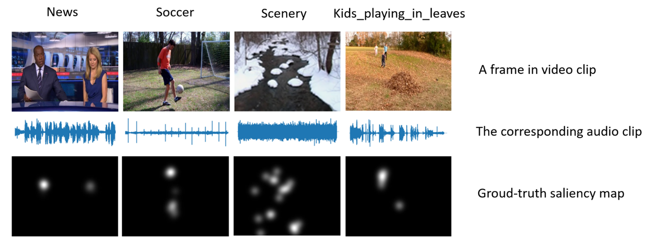
Figure 1. Examples for visualizing the variance of audio and video data.

The exploration of visual contrast information and audio-visual interaction is critical to settle the AVSP task. However, these factors can be easily influenced by the shooting conditions. Objects having relatively higher contrast to background stuffs are more prone to attract attention of humans. The identities of such objects are flexible and vary as the change of shooting scenes. For example, in a speaking video, the mouth region usually draws the highest attention, while the attractive regions are completely different in other social activities such as sport and dance scenes. Visual data differences induced by such factors can degrade the performance of AVSP methods learned with stationary source data. It is likely to contain crucial cues for recognizing salient regions that the audio information accompanying video data. However, the intrinsic attributes of sound data such as pitch, loudness, and timbre are diversified among videos. On the other hand, the relevance between audio and salient regions is variant according to different types of videos. For example, the sound resource locations are usually consistent with salient regions in speaking videos as indicated by the ‘news’ example of Fig. 1; salient regions can not be thoroughly identified out according to sounds in more general social videos like the ‘soccer’ example of Fig. 1; in natural scene videos (‘scenery’ and ‘kids playing in leaves’ of Fig. 1), the audio data is generated by multiple sound resources, and the connection between audio and salient regions is sometimes ambiguous. Due to the above factors, the performance of AVSP methods can be hampered by the domain discrepancy caused by variances of the audio data and the interaction between the audio and the video data.

To deal with the issue of domain discrepancy, we propose a dual domain-adversarial learning framework on the basis of the unsupervised domain adaptation paradigm (Fig. 2 (a)). Following existing methods (tsiami2020stavis, ; yuan2021bio, ), we set up independent branches for extracting features from audio and video inputs respectively. First, an auditory feature domain discriminator is set up to eliminate the impacts of audio data variance. It guides the optimization of the audio feature extraction branch via adversarial training and helps to produce domain-invariant audio features. Then, a cross-modal self-attention module as shown in Fig. 2 (b) is devised to fuse auditory features into visual features extracted by a 3D convolution backbone. The other domain discriminator is adopted to learn fused audio-visual features having a uniform distribution across source and target domains. This is helpful for mitigating the domain discrepancy caused by the variance of visual features and the relation between auditory and visual features. To synthesize the effect of domain discrepancy, we set up two experimental settings: 1) videos captured under different types of scenes are regarded as samples of source and target domains; 2) datasets collected from different sites are regarded as source and target domains. Extensive experiments on two settings demonstrate that our proposed method is effective in making up the performance reduction caused by domain discrepancy.

In summary, the main contributions of this paper are as follows.

• We make an early attempt to tackle the unsupervised domain adaptation problem for audio-visual saliency prediction.

• A dual domain adversarial learning framework is proposed for aligning the audio-visual feature distributions between source and target domains.

• We conduct extensive experiments on cross-scene and cross-dataset adaptation settings, validating the efficacy of our proposed method.

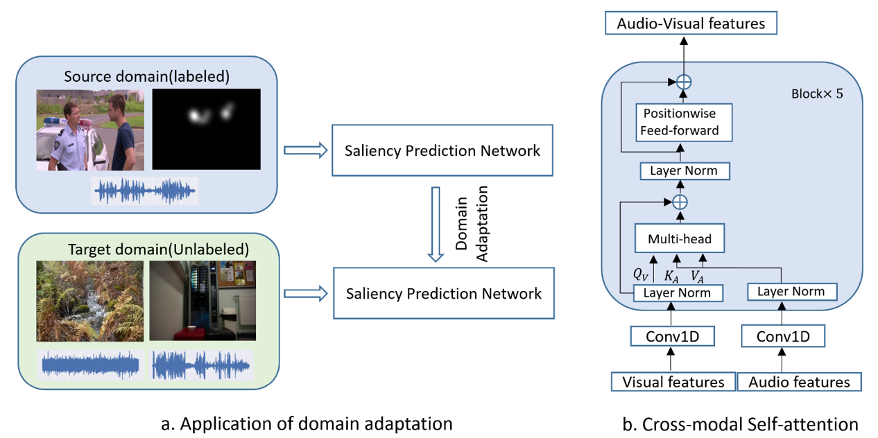
Figure 2. A brief introduction to our proposed method.

2. Related Work

2.1. Video Saliency

With the development of deep convolutional neural networks, a vast number of saliency prediction methods are proposed, and they achieve excellent performance on the image saliency prediction (huang2015salicon, ; zhang2015exploiting, ; pan2017salgan, ; wang2017deep, ) and video saliency prediction (bak2017spatio, ; jiang2018deepvs, ; wang2018revisiting, ; min2019tased, ) task. In video saliency prediction, many recent methods utilize an LSTM to extract spatial and temporal visual features. Wang et al. (wang2018revisiting, ) propose a CNN-LSTM network architecture with an attention mechanism. Linardos et al. (linardos2019simple, ) add a ConvLSTM to an existing neural network and wrap a convolutional layer by using a temporal exponential moving average(EMA) operation. Some existing models have explored 3D-CNN architecture to learn visual features. TASED-Net (min2019tased, ) is a 3D fully-convolutional network, including an encoding network to extract spatiotemporal features and a prediction network to produce a single saliency map. STSConvNet (bak2017spatio, ) extract the temporal and spatial information by using a two-stream network architecture, then fusing them to get a saliency map. Fang et al. (fang2022densely, ) proposed a densely nested top-down flows (DNTDF)-based framework to predict pixel-wise salient object regions. (zhuge2022salient, ) designed an ICON to integrate the features from the micro level and macro level. In (cong2021rrnet, ), a relational reasoning network is proposed for SOD in optical RSIs. (cong2018review, ) review some visual saliency detection algorithms with comprehensive information. Liu et al. (liu2020learning, ) incorporated multi-modal information to learn attention by integrating self-attention and each other’s attention. (zhang2020uc, ) is the first work to employ uncertainty for RGB-D saliency detection, which generates multiple saliency maps by modeling human annotation uncertainty. A survey of RGB-D salient object detection is provided by Zhou et al.(zhou2021rgb, ).

2.2. Audio-Video Saliency

Some early audio-visual saliency prediction methods have been explored for application-specific(ruesch2008multimodal, ; schauerte2011multimodal, ; chen2014audio, ; liao2015audeosynth, ). They employ traditional signal processing techniques for visual saliency and audio localization. Coutrot et al. (coutrot2014audiovisual, ) extract static and dynamic video features by using Gabor filters, then weighing the face regions appropriately and combining the visual saliency map to generate the final audio-visual saliency map. Also, Min et al. (min2016fixation, ) propose an audio-visual model to predict the salient region in the scenes containing moving and sound-generating objects. They generate the saliency map by fusing the audio, spatial, and temporal attention maps.

However, only a few works have explored the end-to-end network for audio-visual saliency fixation prediction based on deep learning. Tavakoli et al. (tavakoli2019dave, ) adopt two 3D-ResNet as the backbone of the two modalities respectively, and their outputs are catenated for encoding. Tsiami et al. (tsiami2020stavis, ) propose STAViS, which employs a multi-modal network that combines visual and auditory information at multiple stages. Furthermore, they investigate the fusion approaches such as computing the cosine similarity, taking the weighted inner product, and bilinear transformation to fuse the audio modality. Jain et al. (jain2020avinet, ) propose a hierarchical structure for audio-video saliency prediction. They analyze three fusion mechanisms, including simple concatenation, bilinear fusion, and transformer-based fusion, to fuse video and audio cues. Zhu et al. (zhu2021lavs, ) propose a lightweight audio-visual saliency model for the audio-visual saliency fixation prediction task. Although these methods show excellent performance, they do not involve the study of unsupervised domain adaptation when the distribution of unlabeled testing data differs from training data.

2.3. Domain Adaptation

Unsupervised domain adaptation(UDA) is targeted at aligning the data distribution of labeled source domain and unlabeled target domain. Thus, the model trained in the source domain can be directly migrated to the target domain without significant performance degradation. The core issue in UDA is how to align the distributions of source and target data. A large number of UDA algorithms have been proposed for classical computer vision tasks such as image classification and semantic segmentation, based on image translation (hoffman2018cycada, ; murez2018image, ), maximum mean discrepancy minimization (wang2020rethink, ), or domain adversarial learning (ganin2015unsupervised, ; liu2021adversarial, ). In this paper, we concentrate on the unsupervised domain adaptation for audio-visual saliency prediction which has not been studied in previous literature.

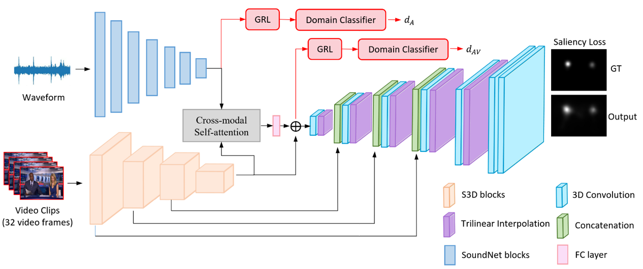
Figure 3. Overall architecture of the proposed model.

3. Method

This paper aims to tackle the unsupervised domain adaptation for AVSP. Assume the source domain data be $\{(\mathbf{A}^{s}_{i},\mathbf{V}^{s}_{i})\}_{i=1}^{N_{s}}$, where $\mathbf{A}^{s}_{i}$ and $\mathbf{V}^{s}_{i}$ denotes the video and audio of the $i$-th sample respectively. $N_{s}$ represents the number of source samples. The ground-truth saliency map for the $i$-th sample in the source dataset is denoted as $\mathbf{G}^{s}_{i}$. For the target data, only a subset of unlabeled samples $\{(\mathbf{A}^{t}_{j},\mathbf{V}^{t}_{j})\}_{j=1}^{N_{t}}$. $N_{t}$ represents the number of target samples. The goal of this paper is to learn a CNN model capable of achieving high AVSP performance on the target domain data. A dual domain adversarial training pipeline is proposed for addressing the above problem. Technical details are introduced in following subsections.

3.1. Architecture Overview

Fig. 3 illustrates the proposed architecture for cross-modal audio-visual saliency prediction. The proposed architecture consists of a visual branch to extract visual features, an audio branch to extract audio features, a cross-modal self-attention module to obtain correlated meaningful audio-visual features for saliency prediction, and a decoder module to decode the audio-visual features and get the final saliency map. Domain adaptation modules are added to make the model learn generalizable features. We input consecutive video frames $\mathbf{V}$ and the corresponding sampled audio sequences $\mathbf{A}$ into the visual and audio branches, respectively, and the final output is a saliency prediction map $\mathbf{P}$. Each domain classifier outputs a binary result to indicate whether the input video comes from the target domain or the source domain.

For visual branch, we use S3D (xie2018rethinking, ) as the backbone to extract visual features. The size of input video frames $\mathbf{V}$ is $C_{0}\times F_{0}\times H_{0}\times W_{0}$, where $F_{0}=32$ is the number of frames and $C_{0}=3$ is the number of frame channels. $H_{0}$ and $W_{0}$ represents the height and width of each frame, respectively. The output of the visual branch is $\mathbf{O}_{\rm V}$. The size of $\mathbf{O}_{\rm V}$ is $C\times F\times H\times W$, where $C=1024$, $F=\frac{F_{0}}{8}$, $H=\frac{H_{0}}{32}$, and $W=\frac{W_{0}}{32}$.

For the audio branch, we adopt SoundNet (aytar2016soundnet, ) to encode the representation of the audio sequence, which is a 1-D fully convolutional network and is initially proposed for audio classification. The size of pre-processed audio sequence $\mathbf{A}$ is $1\times T_{a}\times 1$ , and the size of the output features $\mathbf{O}_{\rm A}$ is $1024\times 3\times 1$.

For audio-visual fusion, inspired by (tsai2019multimodal, ), we use the cross-modal self-attention mechanism to fuse two modalities. $\mathbf{O}_{\rm A}$ and $\mathbf{O}_{\rm V}$ through dimensional changes are input to the cross-modal self-attention fusion module. For the details, see Section 3.2. Then the fusion information goes through a fully-connected layer and is added with $\mathbf{X}_{\rm V}$ to obtain the salient audio-visual features $\mathbf{O}_{\rm AV}$.

Afterwards, $\mathbf{O}_{\rm AV}$ are fed into a decoder consisting of six decoding layers. The first decoding layer contains a 3D convolution and a trilinear interpolation layer. Each of the next three decoding layers contains a concatenation, a 3D convolutional, and a trilinear upsampling layer. The concatenation operation combines the output of the visual block and the output of the last decoder layer along the temporal dimension. The fourth decoding layer is similar to the first layer. The last decoding layer is composed of two 3D convolutional layers, which project the channel and temporal dimension to 1. Finally, the single map goes through a sigmoid activation function to obtain a saliency map $\mathbf{P}$.

Domain adaptation modules are applied to make the knowledge acquired in the labeled source domain to be better generalized in the unlabeled target domain. Specifically, the branch consisting of a gradient reversal layer and a domain classifier is added after the audio output and the output of the fusion module, respectively.

In the following, we mainly describe the cross-modal self-attention mechanism of the fusion module(see Section 3.2) and domain adaptation(see Section 3.3).

3.2. Cross-modal Self-attention

For the fusion of two modalities, previous methods such as computing the cosine similarity between two modalities, simple concatenation, bilinear fusion and so on, can not fully explore the correlation between two modalities. In order to obtain meaningful audio-visual correlation information, we adopt a cross-modal self-attention mechanism, which enables visual modality to receive information from audio modality selectively. The source audio modality is used to reconstruct the information of visual modality and the cross-modal interaction between vision and audio is realized. Details about the cross-modal self-attention are as follows.

The output features of the visual branch $\mathbf{O}_{\rm V}$ are first processed with a max pooling layer and are flattened to $\mathbf{x}_{\rm V}\in{\mathbf{R}^{C\times(HW)}}$. Then the $\mathbf{x}_{\rm V}$ passes through a 1-D convolution and then are collapsed as a vector $\mathbf{X}_{\rm V}\in{\mathbf{R}^{T_{V}\times d_{V}}}$, and the audio features $\mathbf{O}_{\rm A}$ are passed through a 1-D convolution and then are collapsed as a vector $\mathbf{X}_{\rm A}\in{\mathbf{R}^{T_{A}\times d_{A}}}$. Where $T_{V}=H\times W=42$, $T_{A}=3$, and $d_{V}=d_{A}=512$. $T_{(\cdot)}$ is the length of the sequence and $d_{(\cdot)}$ is the feature dimension. The cross-modal attention from $\mathbf{X}_{\rm A}$ to $\mathbf{X}_{\rm V}$ is defined as $\mathbf{Y}_{\rm{A\rightarrow V}}$. The calculation process is as below.

(1) $$\mathbf{Y}_{\rm{A}\rightarrow\rm{V}}=softmax(\frac{\mathbf{Q}_{\rm{V}}\mathbf{K}_{\rm{A}}^{\rm{T}}}{\sqrt{d_{k}}})\mathbf{V}_{\rm{A}}$$

where $\mathbf{Q}_{\rm V}={\mathbf{X}_{\rm V}}{\mathbf{W}_{\rm{Q_{V}}}},\mathbf{\mathbf{K}_{\rm A}={\mathbf{X}_{\rm A}}{\mathbf{W}_{\rm{K_{A}}}}}$ and $\mathbf{V}_{\rm A}={\mathbf{X}_{\rm A}}{\mathbf{W}_{\rm{V_{A}}}}$ represent query, key and value in the cross-modal self-attention module. $\mathbf{W}_{\rm{Q_{V}}}\in{\mathbf{R}^{{d_{V}}\times{d_{k}}}},\mathbf{W}_{\rm{K_{A}}}\in{\mathbf{R}^{{d_{A}}\times{d_{k}}}}$ and $\mathbf{W}_{\rm{V_{A}}}\in{\mathbf{R}^{{d_{A}}\times{d_{v}}}}$ are weights.

In this way, we get the correlation matrix between the audio sequence and the corresponding video, which plays a great role in determining the saliency region of the video. Then, $\mathbf{Y}_{\rm{A\rightarrow V}}$ is added back into $\mathbf{X}_{\rm V}$, and a residual multi-layer perceptron is attached for further feature enhancement. The complete calculation process is illustrated in Fig. 2 (b).

3.3. Domain Adaptation

Our unsupervised domain adaptation module is constituted by a gradient inversion layer and a domain classifier. The gradient inversion layer is located between the feature extraction module and the domain classifier. During the error backpropagation process, this layer reverses the gradient direction, namely making the feature extraction module confuse the domain classifier. Such a manner avoids the two-stage training process of adversarial training. For the domain classifier, three $1\times 1$ spatial convolution layers are adopted to compress the feature dimension. Afterwards, three fully-connected layers are attached, producing the domain classification score.

We setup two separate domain classifiers for audio features and fused audio-visual features respectively. The domain classifier of audio features is denoted as $D_{\rm{A}}$, and that of audio-visual features is denoted as $D_{\rm{AV}}$. Suppose the audio feature and the audio-visual feature extracted from a source domain sample ($\mathbf{A}^{s}$, $\mathbf{V}^{s}$) be $\mathbf{O}^{s}_{\rm{A}}$ and $\mathbf{O}^{s}_{\rm{AV}}$, respectively. $\mathbf{O}^{t}_{\rm{A}}$ and $\mathbf{O}^{t}_{\rm{AV}}$ denotes the audio feature and the audio-visual feature of a target domain sample ($\mathbf{A}^{t}$, $\mathbf{V}^{t}$), respectively. $\mathbf{O}^{s}_{\rm{A}}$ and $\mathbf{O}^{t}_{\rm{A}}$ are fed into the audio domain classifier $D_{\rm{A}}$, resulting in prediction scores $d^{s}_{\rm{A}}$ and $d^{t}_{\rm{A}}$, respectively. On the other hand, $D_{\rm{AV}}$ predicts domain classification scores $d^{s}_{\rm{AV}}$ and $d^{t}_{\rm{AV}}$ from $\mathbf{O}^{s}_{\rm{AV}}$ and $\mathbf{O}^{t}_{\rm{AV}}$, respectively. The domain classification loss for $D_{\rm{A}}$ is defined as $L_{\rm{A}}$ and the loss for $D_{\rm{AV}}$ is $L_{\rm{AV}}$ :

(2) $$L_{\rm{A}}(d^{s}_{\rm{A}},d^{t}_{\rm{A}}) =-\log(d^{s}_{\rm{A}})-\log(1-d^{t}_{\rm{A}}),$$

(3) $$L_{\rm{AV}}(d^{s}_{\rm{AV}},d^{t}_{\rm{AV}}) =-\log(d^{s}_{\rm{AV}})-\log(1-d^{t}_{\rm{AV}}).$$

3.4. Loss Function

The source domain images are employed for training the saliency prediction model with the Kullback-Leibler (KL) divergence. The training loss $L_{s}$ on source domain images is as below:

(4) $$L_{s}(\mathbf{P}^{s},\mathbf{G}^{s})=\sum_{i=1}^{|\mathbf{P}^{s}|}\mathbf{G}^{s}(i)\log(\epsilon+\frac{\mathbf{G}^{s}(i)}{\mathbf{P}^{s}(i)+\epsilon}),$$

where $\mathbf{P}^{s}$ is the saliency map predicted from $\mathbf{A}^{s}$ and $\mathbf{V}^{s}$, $\mathbf{G}$ is the corresponding ground-truth map, and $\epsilon$ is a regularization parameter. $\mathbf{G}^{s}(i)$ and $\mathbf{P}^{s}(i)$ represents the $i$-th pixel of $\mathbf{G}^{s}$ and $\mathbf{P}^{s}$, respectively. $|\mathbf{P}^{s}|$ denotes the number of pixels in $\mathbf{P}^{s}$. The final loss function is formed by summing up (2), (3), and (4):

(5) $$L=L_{s}+L_{\rm{A}}+L_{\rm{AV}}.$$

4. Experiments

In this section, we validate the effectiveness of our method on multiple benchmarks. For evaluating the performance of unsupervised domain adaptation, we synthesize different data domains according to shooting scenarios or dataset sources.

4.1. Datasets and Evaluation Metrics

We carry out the experiments on six audio-visual eye-tracking datasets: DIEM (mital2011clustering, ), AVAD (min2016fixation, ), Coutrot1 (coutrot2014saliency, ), Coutrot2 (coutrot2016multimodal, ), SumMe (gygli2014creating, ), and ETMD (koutras2015perceptually, ). DIEM contains 84 video clips, including commercials, documentaries, game trailers, movie trailers, etc. Coutrot1 contains 60 dynamic nature scene clips such as moving objects, landscapes and faces. Coutrot2 contains 15 clips of 4 people in the meeting. AVAD contains 45 short clips with audio-visual scenes such as dancing, guitar playing, birds singing, etc. ETMD contains 12 videos from six different Hollywood films. SumMe contains 25 unstructured videos. These eye-tracking data are all recorded via the Eyelink eye-tracker from viewers.

Table 1. Number of videos in each dataset.

Dataset	Train	Valid./Test
Faces	30	14
Nature	18	10
Social	58	15

For the evaluation of the domain adaptation, we divide these datasets into two settings based on their shooting scenes. One of the settings is ‘DIEM, AVAD and Coutrot1’, which consists of parts of AVAD, Coutrot1 and DIEM datasets. The three datasets contain multiple scenarios. The other is ‘Faces, Nature and Social’. The three datasets are constructed by selecting data from the existing six datasets according to the content of video frames. ‘Faces’ contains 30 clips with faces, and the corresponding audio is human voice. ‘Nature’ contains 18 clips with landscapes and scenery. ‘Social’ contains 58 clips, including dancing, guitar playing, playing football, etc. The number of videos in each dataset is summarized in Table 1.

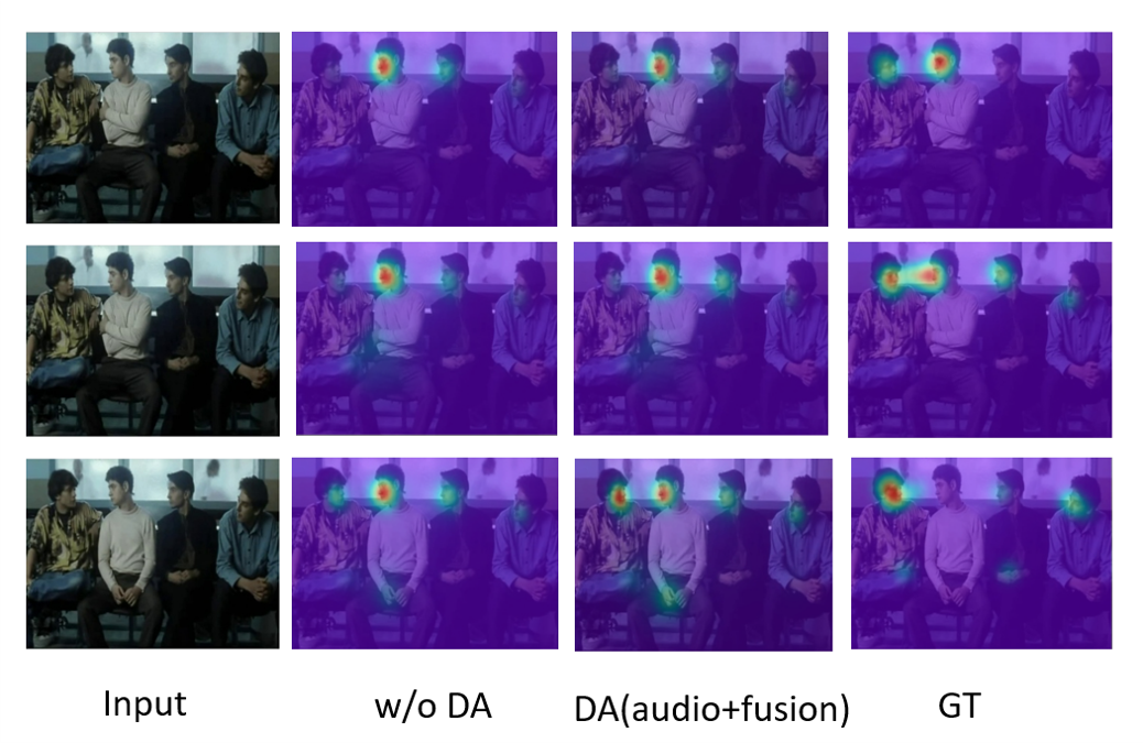
Figure 4. Sample frames from Coutrot1 dataset, and the corresponding ground truth, and saliency maps without adding DA, and adding DA after the audio branch and fusion module.

Table 2. Performance of our proposed method under various domain adaptation settings.

Target data: Nature
Source data	Approach	CC	NSS	sAUC	AUC-J	SIM
Faces	w/o DA	0.4099	1.670	0.5981	0.8442	0.3587
	DA(audio)	0.4352	1.785	0.6021	0.8591	0.3574
	DA(audio + fusion)	0.4488	1.843	0.5988	0.8625	0.3608
Social	w/o DA	0.477	1.9711	0.6019	0.8717	0.3742
	DA(audio)	0.4951	2.064	0.6016	0.8721	0.3964
	DA(audio + fusion)	0.4985	2.084	0.6083	0.8727	0.3833
Source data: AVAD
Target data	Approach	CC	NSS	sAUC	AUC-J	SIM
Coutrot1	w/o DA	0.4685	2.274	0.5881	0.8673	0.3962
	DA(audio)	0.4749	2.298	0.5926	0.8716	0.3962
	DA(audio + fusion)	0.4891	2.364	0.5927	0.8723	0.4057
DIEM	w/o DA	0.5640	2.281	0.6744	0.8857	0.4710
	DA(audio)	0.5692	2.300	0.6782	0.8898	0.4712
	DA(audio + fusion)	0.5758	2.315	0.6797	0.8911	0.4714

We use five evaluation metrics (bylinskii2018different, ), including Linear Correlation Coefficient (CC), AUC-Judd (AUC-J), Similarity Metric (SIM), shuffled AUC (s-AUC), and Normalized Scanpath Saliency (NSS) to evaluate the performance of our model.

4.2. Experimental Setup

In our experiment, for the visual branch, we use the weights pre-trained on DHF1K (wang2018revisiting, ) to initialize the model. For the audio feature extraction network, we initialize the weights from the SoundNet pre-trained in the sound localization task (aytar2016soundnet, ). The learning rate is set to be $10^{-4}$, and the batch size is 8 when training the model without domain adaptation. When adding the domain adaptation, the learning rate is set to be $10^{-5}$, and the batch size is set to 6. In all experiments, we adopt the Adam optimizer to update network parameters.

4.3. Results

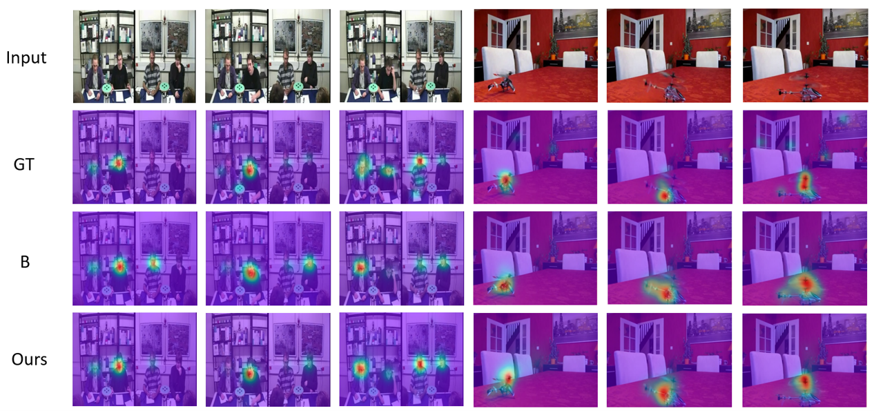
Figure 5. Sample frames from Coutrot2 and Coutrot1 datasets, and the corresponding ground truth, and saliency maps generated by our cross-model self-attention fusion and bilinear fusion for comparisons.

Table 3. Experimental results of using different auditory and visual feature fusion methods. Evaluation metrics are calculated by averaging results on ETMD, SumMe, Coutrot1, Coutrot2, DIEM and AVAD.

Methods	CC	NSS	sAUC	AUC-J	SIM
C	0.6167	3.367	0.6993	0.9155	0.4422
B	0.6090	3.412	0.6965	0.9152	0.4427
CM	0.6138	3.428	0.6757	0.9191	0.4735

Table 4. Comparision results. Evaluation metrics are calculated by averaging results on ETMD, SumMe, Coutrot1, Coutrot2, DIEM and AVAD.

	CC	NSS	sAUC	AUC-J	SIM
STAViS	0.5644	2.9683	0.6584	0.854	0.4345
AViNet	0.6118	3.3683	0.6998	0.9178	0.4445
Ours	0.6138	3.428	0.6757	0.9191	0.4735

We conduct domain adaptation experiments on several different combinations of datasets. Specifically, we take Faces/Social datasets as the source domain, and Nature dataset as the target domain, forming domain adaptation settings: Faces$\rightarrow$Nature and Social$\rightarrow$Nature. The result of not adding the domain adaptation(DA) is tested, denoted by w/o DA, which means the model is trained on the source domain and is tested directly on the target domain. DA(audio) and DA(audio + fusion) represent adding DA after the audio branch and adding DA after the audio branch and fusion module. The results are shown in Table2. Among DIEM, Coutrot1 and AVAD datasets, we take AVAD dataset as the source domain, and DIEM/Coutrot1 datasets as the target domain, forming another two domain adaptation settings: AVAD$\rightarrow$DIEM and AVAD$\rightarrow$Coutrot1. The experimental results are shown in Table 2.

The experimental results show that the performance of the model on the unlabeled target domain datasets is improved by adding DA module. This indicates that the model with DA has learned the domain-invariant characteristics, and the discrepancy between source and target domain is mitigated. We also visualize the results in Fig.4, where the model with DA module performs better.

4.4. Ablation Study

Efficacy of Dual Domain-Adversarial Learning. We analyze the improvement of the model’s performance by adding DA (domain adaptation) in different parts of the model so as to determine the most appropriate position for adding DA. We perform ablation experiments in the following two cases: (1) adding DA after the audio branch (DA(audio)); (2) adding DA after the audio branch and fusion module (DA(audio + fusion)). Table 2 shows the test results of the model in the above two cases. The results show that adding DA after the audio branch and fusion module performs better.

Efficacy of Cross-Modal Self-Attention. We verify the effectiveness of our proposed fusion strategy on six audio-visual datasets by comparing it with existing fusion methods. One is concatenating visual and auditory features, and the other is bilinear fusion. Table 3 shows the averaged evaluation metrics. ‘C’ represents simple concatenation, ‘B’ represents bilinear fusion, and ‘CM’ represents our proposed fusion strategy based on cross-modal self-attention mechanism. It can be seen from Table 3 that the proposed fusion method is superior to other methods on NSS, AUC-J, and SIM, demonstrating the effectiveness of our proposed fusion method. Furthermore, we compare the fusion methods qualitatively. In Fig.5, the first row depicts the sample frames from Coutrot2 and Coutrot1. The ground-truth saliency maps are presented in the second row. The final two rows include the saliency maps generated by bilinear fusion and our cross-model self-attention fusion. As shown in the Figure 5, our results are closer to the ground truth. What’s more, to prove our model’s efficacy without DA for AVSP task, we compare our model with other AVSP methods. Table 4 shows the averaged evaluation metrics on six audio-visual datasets. As is shown, our method obtains better performance on several metrics.

5. Conclusion

In this work, we propose a dual domain-adversarial learning algorithm to solve the problem of unsupervised domain adaptation in audio-visual saliency detection. Specifically, we establish two domain discrimination branches to align the distribution of auditory features and to reduce the domain differences in visual features and audio-visual correlation. Experimental results show that our method can relieve the performance degradation caused by domain discrepancy on the audio-visual saliency prediction task.

- [1] Sophie Marat, Mickäel Guironnet, and Denis Pellerin. Video summarization using a visual attention model. In 2007 15th European Signal Processing Conference, pages 1784–1788. IEEE, 2007.
- [2] Hadi Hadizadeh and Ivan V Bajić. Saliency-aware video compression. IEEE Transactions on Image Processing, 23(1):19–33, 2013.
- [3] Fahad Fazal Elahi Guraya, Faouzi Alaya Cheikh, Alain Tremeau, Yubing Tong, and Hubert Konik. Predictive saliency maps for surveillance videos. In 2010 Ninth International Symposium on Distributed Computing and Applications to Business, Engineering and Science, pages 508–513. IEEE, 2010.
- [4] Hamed R Tavakoli, Ali Borji, Esa Rahtu, and Juho Kannala. Dave: A deep audio-visual embedding for dynamic saliency prediction. arXiv preprint arXiv:1905.10693, 2019.
- [5] Antigoni Tsiami, Petros Koutras, and Petros Maragos. Stavis: Spatio-temporal audiovisual saliency network. In Proceedings of the IEEE/CVF Conference on Computer Vision and Pattern Recognition, pages 4766–4776, 2020.
- [6] Yuan Yuan, Hailong Ning, and Bin Zhao. Bio-inspired audio-visual cues integration for visual attention prediction. arXiv preprint arXiv:2109.08371, 2021.
- [7] Samyak Jain, Pradeep Yarlagadda, Ramanathan Subramanian, and Vineet Gandhi. Avinet: Diving deep into audio-visual saliency prediction. arXiv e-prints, pages arXiv–2012, 2020.
- [8] Yusuf Aytar, Carl Vondrick, and Antonio Torralba. Soundnet: Learning sound representations from unlabeled video. Advances in neural information processing systems, 29, 2016.
- [9] Xun Huang, Chengyao Shen, Xavier Boix, and Qi Zhao. Salicon: Reducing the semantic gap in saliency prediction by adapting deep neural networks. In Proceedings of the IEEE international conference on computer vision, pages 262–270, 2015.
- [10] Jianming Zhang and Stan Sclaroff. Exploiting surroundedness for saliency detection: a boolean map approach. IEEE transactions on pattern analysis and machine intelligence, 38(5):889–902, 2015.
- [11] Junting Pan, Cristian Canton Ferrer, Kevin McGuinness, Noel E O’Connor, Jordi Torres, Elisa Sayrol, and Xavier Giro-i Nieto. Salgan: Visual saliency prediction with generative adversarial networks. arXiv preprint arXiv:1701.01081, 2017.
- [12] Wenguan Wang and Jianbing Shen. Deep visual attention prediction. IEEE Transactions on Image Processing, 27(5):2368–2378, 2017.
- [13] Cagdas Bak, Aysun Kocak, Erkut Erdem, and Aykut Erdem. Spatio-temporal saliency networks for dynamic saliency prediction. IEEE Transactions on Multimedia, 20(7):1688–1698, 2017.
- [14] Lai Jiang, Mai Xu, Tie Liu, Minglang Qiao, and Zulin Wang. Deepvs: A deep learning based video saliency prediction approach. In Proceedings of the european conference on computer vision (eccv), pages 602–617, 2018.
- [15] Wenguan Wang, Jianbing Shen, Fang Guo, Ming-Ming Cheng, and Ali Borji. Revisiting video saliency: A large-scale benchmark and a new model. In Proceedings of the IEEE Conference on Computer Vision and Pattern Recognition, pages 4894–4903, 2018.
- [16] Kyle Min and Jason J Corso. Tased-net: Temporally-aggregating spatial encoder-decoder network for video saliency detection. In Proceedings of the IEEE/CVF International Conference on Computer Vision, pages 2394–2403, 2019.
- [17] Panagiotis Linardos, Eva Mohedano, Juan Jose Nieto, Noel E O’Connor, Xavier Giro-i Nieto, and Kevin McGuinness. Simple vs complex temporal recurrences for video saliency prediction. arXiv preprint arXiv:1907.01869, 2019.
- [18] Chaowei Fang, Haibin Tian, Dingwen Zhang, Qiang Zhang, Jungong Han, and Junwei Han. Densely nested top-down flows for salient object detection. Science China Information Sciences, 65(8):1–14, 2022.
- [19] Mingchen Zhuge, Deng-Ping Fan, Nian Liu, Dingwen Zhang, Dong Xu, and Ling Shao. Salient object detection via integrity learning. IEEE Transactions on Pattern Analysis and Machine Intelligence, 2022.
- [20] Runmin Cong, Yumo Zhang, Leyuan Fang, Jun Li, Yao Zhao, and Sam Kwong. Rrnet: Relational reasoning network with parallel multiscale attention for salient object detection in optical remote sensing images. IEEE Transactions on Geoscience and Remote Sensing, 60:1–11, 2021.
- [21] Runmin Cong, Jianjun Lei, Huazhu Fu, Ming-Ming Cheng, Weisi Lin, and Qingming Huang. Review of visual saliency detection with comprehensive information. IEEE Transactions on circuits and Systems for Video Technology, 29(10):2941–2959, 2018.
- [22] Nian Liu, Ni Zhang, and Junwei Han. Learning selective self-mutual attention for rgb-d saliency detection. In Proceedings of the IEEE/CVF conference on computer vision and pattern recognition, pages 13756–13765, 2020.
- [23] Jing Zhang, Deng-Ping Fan, Yuchao Dai, Saeed Anwar, Fatemeh Sadat Saleh, Tong Zhang, and Nick Barnes. Uc-net: Uncertainty inspired rgb-d saliency detection via conditional variational autoencoders. In Proceedings of the IEEE/CVF conference on computer vision and pattern recognition, pages 8582–8591, 2020.
- [24] Tao Zhou, Deng-Ping Fan, Ming-Ming Cheng, Jianbing Shen, and Ling Shao. Rgb-d salient object detection: A survey. Computational Visual Media, 7(1):37–69, 2021.
- [25] Jonas Ruesch, Manuel Lopes, Alexandre Bernardino, Jonas Hornstein, José Santos-Victor, and Rolf Pfeifer. Multimodal saliency-based bottom-up attention a framework for the humanoid robot icub. In 2008 IEEE International Conference on Robotics and Automation, pages 962–967. IEEE, 2008.
- [26] Boris Schauerte, Benjamin Kühn, Kristian Kroschel, and Rainer Stiefelhagen. Multimodal saliency-based attention for object-based scene analysis. In 2011 IEEE/RSJ International Conference on Intelligent Robots and Systems, pages 1173–1179. IEEE, 2011.
- [27] Yanxiang Chen, Tam V Nguyen, Mohan Kankanhalli, Jun Yuan, Shuicheng Yan, and Meng Wang. Audio matters in visual attention. IEEE Transactions on Circuits and Systems for Video Technology, 24(11):1992–2003, 2014.
- [28] Zicheng Liao, Yizhou Yu, Bingchen Gong, and Lechao Cheng. Audeosynth: music-driven video montage. ACM Transactions on Graphics (TOG), 34(4):1–10, 2015.
- [29] Antoine Coutrot and Nathalie Guyader. An audiovisual attention model for natural conversation scenes. In 2014 IEEE International Conference on Image Processing (ICIP), pages 1100–1104. IEEE, 2014.
- [30] Xiongkuo Min, Guangtao Zhai, Ke Gu, and Xiaokang Yang. Fixation prediction through multimodal analysis. ACM Transactions on Multimedia Computing, Communications, and Applications (TOMM), 13(1):1–23, 2016.
- [31] Dandan Zhu, Defang Zhao, Xiongkuo Min, Tian Han, Qiangqiang Zhou, Shaobo Yu, Yongqing Chen, Guangtao Zhai, and Xiaokang Yang. Lavs: A lightweight audio-visual saliency prediction model. In 2021 IEEE International Conference on Multimedia and Expo (ICME), pages 1–6. IEEE, 2021.
- [32] Judy Hoffman, Eric Tzeng, Taesung Park, Jun-Yan Zhu, Phillip Isola, Kate Saenko, Alexei Efros, and Trevor Darrell. Cycada: Cycle-consistent adversarial domain adaptation. In International conference on machine learning, pages 1989–1998. PMLR, 2018.
- [33] Zak Murez, Soheil Kolouri, David Kriegman, Ravi Ramamoorthi, and Kyungnam Kim. Image to image translation for domain adaptation. In Proceedings of the IEEE Conference on Computer Vision and Pattern Recognition, pages 4500–4509, 2018.
- [34] Wei Wang, Haojie Li, Zhengming Ding, and Zhihui Wang. Rethink maximum mean discrepancy for domain adaptation. arXiv preprint arXiv:2007.00689, 2020.
- [35] Yaroslav Ganin and Victor Lempitsky. Unsupervised domain adaptation by backpropagation. In International conference on machine learning, pages 1180–1189. PMLR, 2015.
- [36] Xiaofeng Liu, Zhenhua Guo, Site Li, Fangxu Xing, Jane You, C-C Jay Kuo, Georges El Fakhri, and Jonghye Woo. Adversarial unsupervised domain adaptation with conditional and label shift: Infer, align and iterate. In Proceedings of the IEEE/CVF International Conference on Computer Vision, pages 10367–10376, 2021.
- [37] Saining Xie, Chen Sun, Jonathan Huang, Zhuowen Tu, and Kevin Murphy. Rethinking spatiotemporal feature learning: Speed-accuracy trade-offs in video classification. In Proceedings of the European conference on computer vision (ECCV), pages 305–321, 2018.
- [38] Yao-Hung Hubert Tsai, Shaojie Bai, Paul Pu Liang, J Zico Kolter, Louis-Philippe Morency, and Ruslan Salakhutdinov. Multimodal transformer for unaligned multimodal language sequences. In Proceedings of the conference. Association for Computational Linguistics. Meeting, volume 2019, page 6558. NIH Public Access, 2019.
- [39] Parag K Mital, Tim J Smith, Robin L Hill, and John M Henderson. Clustering of gaze during dynamic scene viewing is predicted by motion. Cognitive computation, 3(1):5–24, 2011.
- [40] Antoine Coutrot and Nathalie Guyader. How saliency, faces, and sound influence gaze in dynamic social scenes. Journal of vision, 14(8):5–5, 2014.
- [41] Antoine Coutrot and Nathalie Guyader. Multimodal saliency models for videos. In From Human Attention to Computational Attention, pages 291–304. Springer, 2016.
- [42] Michael Gygli, Helmut Grabner, Hayko Riemenschneider, and Luc Van Gool. Creating summaries from user videos. In European conference on computer vision, pages 505–520. Springer, 2014.
- [43] Petros Koutras and Petros Maragos. A perceptually based spatio-temporal computational framework for visual saliency estimation. Signal Processing: Image Communication, 38:15–31, 2015.
- [44] Zoya Bylinskii, Tilke Judd, Aude Oliva, Antonio Torralba, and Frédo Durand. What do different evaluation metrics tell us about saliency models? IEEE transactions on pattern analysis and machine intelligence, 41(3):740–757, 2018.