Quadrotor Autonomous Landing on Moving Platform

Abstract

This paper introduces a quadrotor’s autonomous take-off and landing system on a moving platform. The designed system addresses three challenging problems: fast pose estimation, restricted external localization, and effective obstacle avoidance. Specifically, first, we design a landing recognition and positioning system based on the AruCo marker to help the quadrotor quickly calculate the relative pose; second, we leverage a gradient-based local motion planner to generate collision-free reference trajectories rapidly for the quadrotor; third, we build an autonomous state machine that enables the quadrotor to complete its take-off, tracking and landing tasks in full autonomy; finally, we conduct experiments in simulated, real-world indoor and outdoor environments to verify the system’s effectiveness and demonstrate its potential.

I INTRODUCTION

In recent years, quadrotor Unmanned Aerial Vehicles (UAVs) that can take off and land vertically (VTOL) have played a key role in power line inspection, express delivery, and farmland sowing due to their flexibility and ease of deployment [1][2][3]. Among them, autonomous take-off and landing technology without external positioning (e.g. GPS and motion capture) is an important part, which is essential for UAVs to perform more complex tasks and cooperate with ground mobile robots.

Sani et al. [4] proposed a visual and inertial navigation method combined with Kalman filter and proportional-integral-derivative (PID) controller to achieve relative pose estimation and accurate UAV landing on ground QR code. To estimate the state quantities of dynamic targets and track them efficiently, Lee et al. [5] adopted an image-based visual servoing method in two-dimensional space to generate reference velocity commands, which were fed to an adaptive sliding mode controller while considering an adaptive rule for the ground effect in landing process. However, these methods could only achieve static and very low-speed autonomous landing and at the same time only indoor experimental verification.

Accurate position estimation of UAV and landing platform is necessary for autonomous landing. Mellinger et al. [6] designed robust quadrotor planning and control algorithms for UAV’s perching and landing, but they needed a VICON motion capture system to track the quadrotor as well as the landing surfaces. Daly et al. [7] proposed a coordinated landing control scheme. In their method, they used a joint decentralized controller to reach the rendezvous point for landing and the controller performed stably in the presence of delay. However, their approach relied on expensive Real-Time Kinematic (RTK) GPS on both UAV and Unmanned Ground Vehicle (UGV) for sub-centimeter positioning. The reliance on external positioning systems was not practical in many scenarios.

To let the UAV land on a fast-moving target, Borowczyk et al. used Kalman filtering to calculate the accurate pose of the UAV relative to the landing pad by fusing multiple sources of measurement information. They used the proportional (P) controller in the distance and the proportional-derivative (PD) controller in the near, and the mobile platform could reach a high speed at 30km/h [8]. However, the UAV did not perform motion planning when tracking and landing, which means that when there are obstacles on the way, it may cause collisions because the UAV cannot avoid obstacles.

To address the challenges mentioned above, the main contributions of this paper are summarized as follows:

(1) We design a landing positioning system based on AruCo squared fiducial marker [9] to be placed on the moving platform. The UAV can detect and calculate the pose relative to the UGV quickly, accurately and at a low cost.

(2) We utilize a gradient-based local motion planning method [10] to generate a collision-free, smooth and feasible reference trajectory for UAV in tracking and landing.

(3) We design an automatic state machine that enables UAV to achieve take-off, tracking and landing missions.

The rest of this paper is organized as follows. We first introduce the UAV-UGV system in Section II and then present the detection and positioning of the mobile landing platform in Section III. Furthermore, we demonstrate the local motion planning algorithm and landing state machine in Section IV. Finally, in Section V and Section VI, we conduct experiments, analyze the results and give future plans.

II QUADROTOR SYSTEM DESIGN

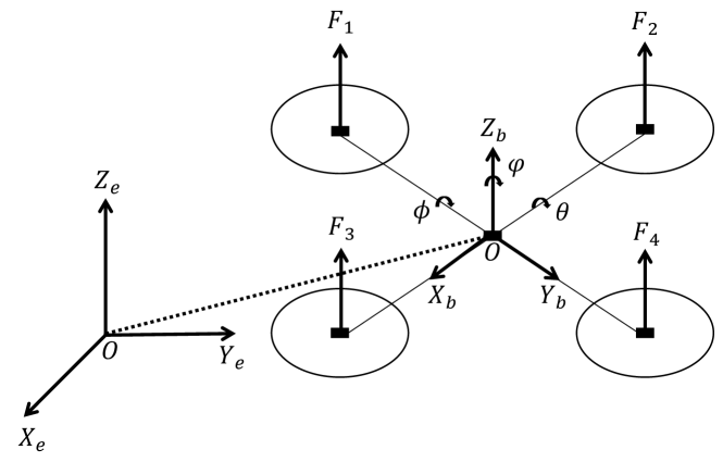
Figure 1: Coordinate systems of a quadrotor.

II-A Modeling

In this paper, it is assumed that the quadrotor is a rigid body with uniform mass distribution and axisymmetric, the mass and rotational inertia are constant, and the center of gravity coincides with the geometric center, as shown in Fig. 1. $p=\left[x\,\,y\,\,z\right]^{T}$ represents the position of quadrotor. $v=\left[v_{x}\,\,v_{y}\,\,v_{z}\right]^{T}$ and $\omega=\left[\omega_{x},\omega_{y},\omega_{z}\right]^{T}$ denote velocity and angular velocity, respectively. The roll/pitch/yaw angle of a quadrotor is represented by $\boldsymbol{\phi}=\left[\varphi,\,\,\theta,\,\,\psi\right]^{T}$. There are two coordinate systems: world inertial frame $E_{q}=\left\{e_{x},e_{y},e_{z}\right\}$ and body-fixed frame $B_{q}=\left\{b_{x},b_{y},b_{z}\right\}$. The transformation between two coordinate systems is represented by

$$R_{b}=$$ (1)

$$\left[\begin{matrix}C\theta C\psi&-C\phi S\psi+S\phi S\theta C\psi&S\phi S\psi+C\phi S\theta C\psi\\ C\theta S\psi&C\phi C\psi+S\phi S\theta S\psi&-S\phi C\psi+C\phi S\theta S\psi\\ -S\theta&S\phi C\theta&C\phi C\theta\\ \end{matrix}\right]$$

According to the Newton-Euler equation, the position and attitude dynamics equation of the quadrotor is expressed as follows [11]:

$$\begin{cases}\dot{v}_{x}=-\frac{T}{m}\left[\left(sin\phi sin\psi+cos\phi sin\theta cos\psi\right)+F_{x}^{drag}\right]\\ \dot{v}_{y}=-\frac{T}{m}\left[\left(-sin\phi cos\psi+cos\phi sin\theta sin\psi\right)+F_{y}^{drag}\right]\\ \dot{v}_{z}=-\frac{T}{m}\left[cos\phi cos\theta+F_{z}^{drag}+mg\right]\\ \end{cases}$$ (2)

$$\begin{cases}\dot{\omega}_{x}=\frac{1}{I_{xx}}\left[\left(I_{yy}-I_{zz}\right)\omega_{y}\omega_{z}+\tau_{x}^{motor}+J_{r}\varOmega\omega_{y}\right]\\ \dot{\omega}_{y}=\frac{1}{I_{yy}}\left[\left(I_{zz}-I_{xx}\right)\omega_{x}\omega_{z}+\tau_{y}^{motor}-J_{r}\varOmega\omega_{x}\right]\\ \dot{\omega}_{z}=\frac{1}{I_{zz}}\left[\left(I_{xx}-I_{yy}\right)\omega_{x}\omega_{y}+\tau_{z}^{motor}\right]\\ \end{cases}$$ (3)

where $T=c_{T}\varpi^{2}$ is the thrust of the motor, $F^{drag}$ is air resistance, $I_{i}$ and $\tau_{i}^{motor}$ denote inertial and torque, respectively.

The position and attitude motion equation of the quadrotor can be written as

$$\dot{p}=v$$ (4)

$$\left[\begin{array}[]{c}\dot{\phi}\\ \dot{\theta}\\ \dot{\psi}\\ \end{array}\right]=\left[\begin{matrix}1&sin\phi tan\theta&cos\phi tan\theta\\ 0&cos\phi&-sin\phi\\ 0&sin\phi/cos\theta&cos\phi/cos\theta\\ \end{matrix}\right]\left[\begin{array}[]{c}\omega_{x}\\ \omega_{y}\\ \omega_{z}\\ \end{array}\right]$$ (5)

II-B Hardware Setup

In this paper, we use a P450 quadrotor designed by Amovlab and a Husky A200 UGV built by Clearpath, as shown in Fig. 2. The core components of the quadrotor include open source autopilot hardware Pixhawk [12], software PX4 flight control [13], onboard computer NVIDIA Jetson NX, monocular wide-angle camera, Intel Realsense T265 tracking camera and Intel Realsense D435i depth camera.

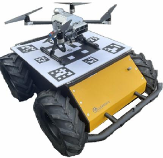
Figure 2: UAV-UGV system.

II-C State Estimation

PX4 provides an Extended Kalman Filter (EKF) [14] -based algorithm to process sensor measurements and calculate an estimate of flight states, as shown in Fig. 3. In order to get more accurate pose information and use it in a GPS-denied environment, we use the off-the-shelf Visual-Inertial Odometry (VIO) method in Intel Realsense T265 to obtain pose information of the UAV relative to the take-off point.

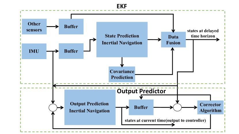
Figure 3: UAV state estimation.

II-D Flight Controller

A standard cascaded control architecture is recommended in PX4 for multirotor and the controllers are a mix of P and PID controllers, as shown in Fig. 4. The controller consists of position control and attitude control. Inside the controller, the outer loop is for position (angle) control and the inner loop is for acceleration (angular velocity) control. The inner loop responds faster than the outer loop and acts directly on the motor; hence the inner loop parameters are vital when adjusting the controller parameters. In the offboard mode of PX4, position, velocity, angle and angular velocity can be controlled separately.

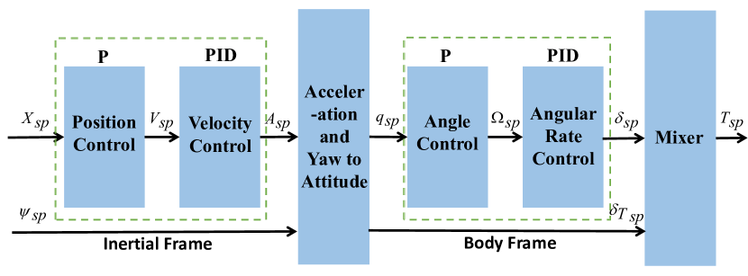
Figure 4: PX4 cascaded PID controller.

III DETECTION AND LOCALIZATION OF LANDING PLATFORM

In this section, we introduce the detection of the landing platform and the calculation of the relative pose relationship between the UAV and the UGV, which is crucial to achieving a reliable landing.

III-A Pinhole Camera Calibration

For the purpose of mapping objects in three-dimensional space to two-dimensional camera space, we achieve pinhole camera calibration [15] to establish the geometric model of a specific camera. The geometric model parameters are called camera parameters, including intrinsic and extrinsic parameters.

$$Z\left[\begin{array}[]{c}u\\ v\\ 1\\ \end{array}\right]=\left(\begin{matrix}f_{x}&\gamma&c_{x}\\ 0&f_{y}&c_{y}\\ 0&0&1\\ \end{matrix}\right)\left[\begin{matrix}R_{3\times 3}&t_{3\times 1}\\ \end{matrix}\right]\left[\begin{array}[]{c}X\\ Y\\ Z\\ 1\\ \end{array}\right]$$ (6)

III-B Landing Pad Detection

Figure 5: AruCo marker-based landing pad.

In this paper, we use the AruCo squared fiducial marker library [9] for target detection. We implement the detection of markers in OpenCV [16], which includes three steps: using adaptive thresholding to obtain borders, using polygonal approximation and removing too close rectangles, performing marker identification. The AruCo landing pad design is inspired by Qi et al. [17], which consists of four different sizes and ten kinds of markers, as shown in Fig. 5. These markers ensure that the moving platform can be seen near, far and sideways. The actual scale of each AruCo marker and its accurate relative relationship with other surrounding markers are significant. For a more accurate landing, we define and test markers’ maximum detectable and active distance ranges, as shown in Tab. I. The maximum distance range and offset means the maximum x, y, z distance of the UAV from the center of a specific marker when the UAV can detect that specific marker. The active range is a subset of the maximum range, which means the distance at which the marker at a specific location plays a major role in calculating relative pose.

TABLE I: Marker detection range

Marker type No.	Max detectable z-distance range	Max (x,y) offset
43 (2.5 cm)	(Land,0.15) m	(0.15,0.15) m
5-8 (6.4 cm)	(Land,0.50) m	(0.39,0.39) m
1-4 (9.5 cm)	(Land,1.15) m	(0.90,0.90) m
68 (25.7 cm)	(Land,3.00) m	(1.42,1.42) m
Marker type No.	Active z-distance range	Active (x,y) offset
43 (2.5 cm)	(Land,0.15) m	(0.15,0.15) m
5-8 (6.4 cm)	(0.20,0.30) m	(0.00,0.20-0.39) m
1-4 (9.5 cm)	(0.40,1.00) m	(0.70,0.70) m
68 (25.7 cm)	(1.00,3.00) m	-

III-C 3D Pose Estimation

Knowing n reference 3D points and corresponding 2D projections, we can construct the Perspective-n-Point (PNP) problem to estimate the camera’s pose relative to the moving platform. When solving the PNP problem, similar to [17], we use the nonlinear optimization method Bundle Adjustment to minimize the re-projection error and then estimate the rotation and translation between the camera coordinates and the marker coordinates. Through coordinate transformation, the coordinates in the landing pad system $M_{q}=\left\{m_{x},m_{y},m_{z}\right\}$ can be transformed into the camera coordinate system $C_{q}=\left\{c_{x},c_{y},c_{z}\right\}$, body-fixed coordinate system $B_{q}$ and the world inertial system (ENU) $E_{q}$ successively. Finally, the pose estimation of the UAV relative to the landing platform is expressed as

$$P^{b}=R_{C}^{B}\left(\left(R_{M}^{C}P^{m}+t_{M}^{C}\right)+Offset^{c}\right)$$ (7)

where $P,R,t$ denotes position, rotation and translation in different coordinate frames, respectively and $Offset^{c}$ is the known camera mount offset.

IV PLANNING ALGORITHM AND LANDING STATE MACHINE

Our paper uses a gradient-based local motion planning method [10] [18], which does not need to construct the Euclidean Signed Distance Field (ESDF) in advance and therefore greatly reduces the planning time. Constructing the ESDF field takes not only plenty of time but also the trajectory calculated by the ESDF may fall into a local minimum. The method includes three steps: trajectory initialization, gradient-based trajectory optimization, time re-assignment and trajectory refinement.

IV-A Front-end B-Spline Initialization

In the initialization phase, a uniform B-Spline curve $\phi$ that satisfies the final constraints but does not consider obstacles is generated. An estimate of the collision force is performed and for each segment of the track where collision is detected, the A* algorithm is used to generate a collision-free path $\varGamma$. Then for each control point $Q_{i}$ of the collision line, an anchor point $P_{ij}$ is generated on the obstacle surface and the distance from $Q_{i}$ to the $jth$ obstacle is set as: $d_{ij}=\left(Q_{i}-P_{ij}\right)V_{ij}$, where $V_{ij}$ are unit vectors from $Q_{i}$ to $P_{ij}$.

IV-B Back-end Trajectory Optimization

The B-spline curve of the front-end part is uniquely determined by the degree $p_{b}$, $N_{c}$ control points $\left\{Q_{1},Q_{2},\cdots,Q_{N}\right\}$, and vector $\left[t_{1},t_{2},\cdots,t_{M}\right]$. The optimization problem is modeled as $min_{Q}J=\lambda_{s}J_{s}+\lambda_{c}J_{c}+\lambda_{d}J_{d}$. In the formula, $J_{s},J_{c},J_{d}$ represents smoothness term, collision term, dynamic feasibility term, respectively and $\lambda_{s},\lambda_{c},\lambda_{f}$ is the corresponding coefficient. According to the convex hull property, the smoothness cost $J_{s}$ and feasibility cost $J_{d}$ is set as

$$J_{s}=\sum_{i=1}^{N_{c}-2}{\lVert A_{i}\rVert_{2}^{2}}+\sum_{i=1}^{N_{c}-3}{\lVert J_{i}\rVert_{2}^{2}}$$ (8)

$$J_{d}=\sum_{i=1}^{N_{c}-1}{\omega_{v}F\left(V_{i}\right)}+\sum_{i=1}^{N_{c}-2}{\omega_{a}F\left(A_{i}\right)}+\sum_{i=1}^{N_{c}-3}{\omega_{j}F\left(J_{i}\right)}$$ (9)

where $A_{i}$ is acceleration, $J_{i}$ is jerk, $\omega_{i,i=v,a,j}$ are weights and $F\left(\cdot\right)$ is a two-order continuously differentiable function of control points. Collision cost $J_{c}$ pushes control points until $d_{ij}>s_{f}$(safe distance) and it is defined as

$$J_{c}=\sum_{i=1}^{N_{c}}{j_{c}\left(Q_{i}\right)}$$ (10)

where $j_{c}\left(\cdot\right)$ is also a two-order continuously differentiable function.

IV-C Time Re-assignment and Trajectory Refinement

An additional time re-assignment step is necessary to avoid aggressive motion and ensure that the trajectory satisfies the kinodynamic constraints. Then, an curve fitting method is presented to make the refined trajectory $\varPhi_{f}$ maintain an almost identical shape to the original trajectory $\varPhi_{s}$. After obtaining the initial value of $\varPhi_{f}$, the refined optimization problem is defined as $min_{Q}J=\lambda_{s}J_{s}+\lambda_{c}J_{c}+\lambda_{f}J_{f}$ and the third term $\lambda_{f}J_{f}$ is the curve fitting term, which is defined as

$$J_{f}=\int_{0}^{1}{\left(\frac{d_{\alpha}\left(\alpha\right)^{2}}{a^{2}}+\frac{d_{r}\left(\alpha\right)^{2}}{b^{2}}\right)}d\alpha$$ (11)

where $d_{\alpha}\left(\alpha\right)$ and $d_{r}\left(\alpha\right)$ represents axial and radial displacement of two curves, respectively. $a$ is set to 20 and $b$ is set to 1.

IV-D Landing State Machine

The UAV’s autonomous take-off and landing task is driven by an autonomous state machine, as shown in Fig. 6. The main steps are as follows: UAV takes off and flies to a preset point; UAV hovers and waits for the landing target to appear; UAV sees the landing point and calculates the relative pose; UAV’s planner plans a reference trajectory in real-time; UAV’s cascade PID controller tracks the generated trajectory; UAV meets the landing conditions, descends, and completes the landing task. It is worth noting that because the target point is moving, the UAV usually does not entirely execute the trajectory given by the planner, and will instead execute a new reference trajectory.

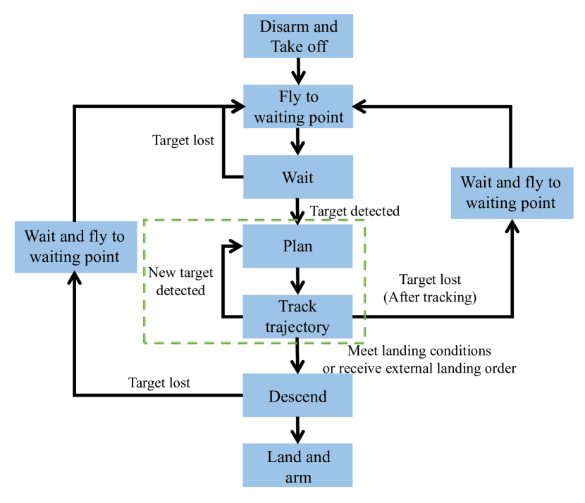
Figure 6: Landing state machine.

V EXPERIMENTS AND RESULTS

In this section, we test our method in both simulation and real-world experimental environments.

V-A Simulation Experiments

We conduct simulation experiments on the ROS/Gazebo platform named Prometheus and we also use part of the ROS packages provided by Prometheus in real-world experiments.

The UAV takes off to the pre-set point $\left(-4.0,-2.0,4.5\right)$ and waits to detect the landing platform. After detecting the UGV, the UAV continuously plans the trajectory and tracks it. Then UAV descends and when the height from the landing point is less than 0.6m, it starts to land and completes the landing. The trajectory of UAV is shown in Fig. 7 and main flight data is shown in Tab. II.

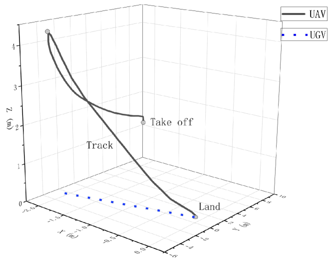
Figure 7: Simulation trajectory. Target speed: 2.8 km/h.

TABLE II: Key Flight Data

Experiment	Distance	Target Speed	UAV Max Speed	UAV Average Speed	Planning Time
Simulation	20 m	2.8 km/h	4.1 km/h	0.8 km/h	4.75 ms
Indoor 1	5.2 m	0.0 km/h	4.8 km/h	0.4 km/h	0.83 ms
Indoor 2	3.7 m	0.8 km/h	2.1 km/h	0.3 km/h	1.60 ms
Outdoor 1	12.9 m	2.16 km/h	6.6 km/h	2.7 km/h	3.16 ms
Outdoor 2	14.3 m	3.24 km/h	8.2 km/h	3.3 km/h	3.49 ms

V-B Real-world Experiments

V-B1 Indoor Environment

We first conduct experiments on static and dynamic targets in indoor environments. The UAV can accurately land on the target within the field of view. In a moving target experiment, the UGV moves linearly in the positive direction of the y-axis at a speed of 0.8 km/h. After the UAV takes off to the target point $\left(0.0,0.0,0.75\right)$, it starts to follow, and when the landing conditions are satisfied (tracking distance over 2.5m or external landing command), it begins to descend to 0.2m, and then quickly lands. The trajectory of the UAV and UGV is shown in Fig. 8 and the experimental data is shown in Tab. II.

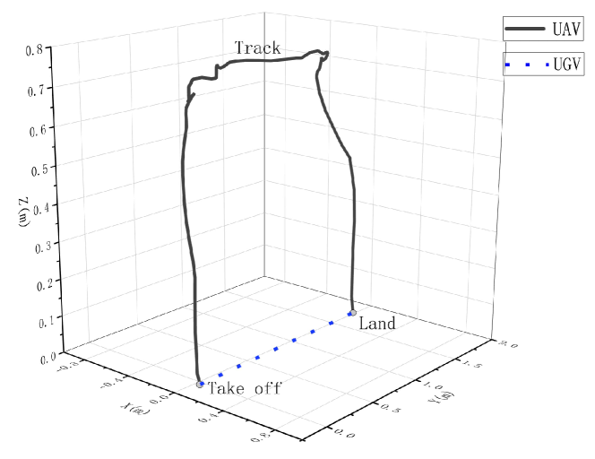
Figure 8: Indoor experiment trajectory. Target speed: 0.8 km/h.

V-B2 Outdoor Environment with Wind Speed

We then conduct dynamic target landing experiments in an outdoor environment with wind speed, as shown in Fig. 9.

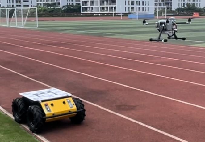
Figure 9: Outdoor environment.

Similar to the indoor experiment, the UGV moves at a linear speed of 2.16 km/h and 3.24 km/h, respectively; the UAV first takes off to a preset point $\left(0.0,0.0,1.0\right)$, then follows, and when an external landing command is received, the UAV quickly lands. The trajectory of the UAV-UGV system is shown in Fig. 10 and the critical data is also shown in Tab. II.

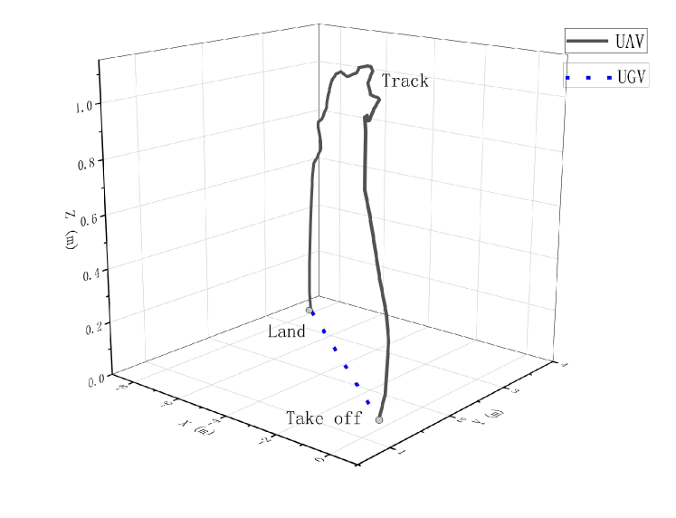
Figure 10: Outdoor experiment trajectory. Target speed: 3.24 km/h.

V-B3 Trajectory Analysis

It can be seen from the trajectory graph that the trajectory in the simulation is relatively smooth. Although the motion planner gives a smooth reference trajectory, the actual flight trajectory of the UAV in the real situation slightly oscillates. This is because the robot’s actuators, including motors, have uncertainties from control noise, wear, and mechanical failures [19].

V-C Obstacle Avoidance Demonstration

We use the local motion planner in [10] and provide the UAV with collision-free, smooth and feasible trajectories. In the experiment, there is a $60cm\times 120cm\times 120cm$ obstacle in front of the UAV. The UAV bypasses the obstacle, and then sees and lands on the platform, as shown in Fig. 11.

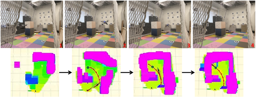
Figure 11: Obstacle avoidance and trajectory update demonstration.

Crucial planning data is shown in Tab. III, where the Obstacle Density is the proportion of obstacles per square meter.

TABLE III: Obstacle Avoidance

Flight Time	Flight Distance	Obstacle Density	Planning Time	Re-planning Times
58 s	10.2 m	0.11$/m^{2}$	2.40 ms	5 times

V-D Parameters Setting Analysis

We analyze and tune the prime parameters of the motion planner, as shown in Tab. IV. Resolution is the resolution of the grid map of the surrounding environment built from the depth information and Obstacles Inflation is the relative size of the inflation of the obstacles. $\lambda$ is the coefficient of each loss item in the loss function described in IV. For the sake of safety, the collision $\lambda_{collision}$ in our paper is set relatively large.

TABLE IV: Planner Parameters

Resolution	Obstacles Inflation	$\lambda_{smooth}$	$\lambda_{collision}$	$\lambda_{feasibility}$	$\lambda_{fitness}$
0.15	0.299	1.0	8.5	0.1	1.0

V-E Comparison Results

We compare our method with previous work in autonomous landing to verify the effectiveness of our method. The relevant comparison results are shown in Tab. V. Compared with the previous methods, our system can realize the autonomous take-off and landing of a quadrotor on a UGV platform in different scenarios without external positioning and can avoid static obstacles simultaneously.

TABLE V: Comparison Results with Related Works

Work	Target Speed	Obstacle Avoidance	External Localization	Environment
Sani et al.	0.0 km/h	No	No need	Indoor
Lee et al.	0.25 km/h	No	No need	Indoor
Mellinger et al.	0.0 km/h	No	Need	Indoor
Daly et al.	3.6 km/h	No	Need	Outdoor
Ours	3.24 km/h	Yes	No need	Indoor/Outdoor

VI CONCLUSIONS AND FUTURE WORK

In this paper, we present a quadrotor system in the above sections. In order to detect the target quickly and accurately, we design an AruCo-based landing pad system. We utilize a gradient-based local motion planner to rapidly generate collision-free, smooth, and kinodynamic feasible reference trajectories. We then present an automatic state machine to achieve full autonomy in take-off and landing tasks. Experiments show that our system could realize the autonomous landing task on a mobile platform in real outdoor environments.

In the future, we will focus on more high-speed and more uncertain moving target landing tasks, while focusing on improving the accuracy of landing.

References

- [1] S. Gupte, P. I. T. Mohandas, and J. M. Conrad, “A survey of quadrotor unmanned aerial vehicles,” in 2012 Proceedings of IEEE Southeastcon, pp. 1–6, IEEE, 2012.
- [2] D. Zhu, Y. Du, Y. Lin, H. Li, C. Wang, X. Xu, and M. Q.-H. Meng, “Hawkeye: Open source framework for field surveillance,” in 2017 IEEE/RSJ International Conference on Intelligent Robots and Systems (IROS), pp. 6083–6090, IEEE, 2017.
- [3] T. Li, C. Wang, C. W. de Silva, et al., “Coverage sampling planner for uav-enabled environmental exploration and field mapping,” in 2019 IEEE/RSJ International Conference on Intelligent Robots and Systems (IROS), pp. 2509–2516, IEEE, 2019.
- [4] M. F. Sani and G. Karimian, “Automatic navigation and landing of an indoor ar. drone quadrotor using aruco marker and inertial sensors,” in 2017 international conference on computer and drone applications (IConDA), pp. 102–107, IEEE, 2017.
- [5] D. Lee, T. Ryan, and H. J. Kim, “Autonomous landing of a vtol uav on a moving platform using image-based visual servoing,” in 2012 IEEE international conference on robotics and automation, pp. 971–976, IEEE, 2012.
- [6] D. Mellinger, M. Shomin, and V. Kumar, “Control of quadrotors for robust perching and landing,” in Proceedings of the International Powered Lift Conference, pp. 205–225, 2010.
- [7] J. M. Daly, Y. Ma, and S. L. Waslander, “Coordinated landing of a quadrotor on a skid-steered ground vehicle in the presence of time delays,” Autonomous Robots, vol. 38, no. 2, pp. 179–191, 2015.
- [8] A. Borowczyk, D.-T. Nguyen, A. P.-V. Nguyen, D. Q. Nguyen, D. Saussié, and J. Le Ny, “Autonomous landing of a quadcopter on a high-speed ground vehicle,” Journal of Guidance, Control, and Dynamics, vol. 40, no. 9, pp. 2378–2385, 2017.
- [9] F. J. Romero-Ramirez, R. Muñoz-Salinas, and R. Medina-Carnicer, “Speeded up detection of squared fiducial markers,” Image and vision Computing, vol. 76, pp. 38–47, 2018.
- [10] X. Zhou, Z. Wang, H. Ye, C. Xu, and F. Gao, “Ego-planner: An esdf-free gradient-based local planner for quadrotors,” IEEE Robotics and Automation Letters, vol. 6, no. 2, pp. 478–485, 2020.
- [11] P. Pounds, R. Mahony, and P. Corke, “Modelling and control of a quad-rotor robot,” in Proceedings of the 2006 Australasian Conference on Robotics and Automation, pp. 1–10, Australian Robotics and Automation Association (ARAA), 2006.
- [12] L. Meier, P. Tanskanen, F. Fraundorfer, and M. Pollefeys, “Pixhawk: A system for autonomous flight using onboard computer vision,” in 2011 IEEE International Conference on Robotics and Automation, pp. 2992–2997, IEEE, 2011.
- [13] L. Meier, D. Honegger, and M. Pollefeys, “Px4: A node-based multithreaded open source robotics framework for deeply embedded platforms,” in 2015 IEEE international conference on robotics and automation (ICRA), pp. 6235–6240, IEEE, 2015.
- [14] M. I. Ribeiro, “Kalman and extended kalman filters: Concept, derivation and properties,” Institute for Systems and Robotics, vol. 43, p. 46, 2004.
- [15] Z. Zhang, “A flexible new technique for camera calibration,” IEEE Transactions on pattern analysis and machine intelligence, vol. 22, no. 11, pp. 1330–1334, 2000.
- [16] G. Bradski and A. Kaehler, Learning OpenCV: Computer vision with the OpenCV library. " O’Reilly Media, Inc.", 2008.
- [17] Y. Qi, J. Jiang, J. Wu, J. Wang, C. Wang, and J. Shan, “Autonomous landing solution of low-cost quadrotor on a moving platform,” Robotics and Autonomous Systems, vol. 119, pp. 64–76, 2019.
- [18] X. Zhou, J. Zhu, H. Zhou, C. Xu, and F. Gao, “Ego-swarm: A fully autonomous and decentralized quadrotor swarm system in cluttered environments,” in 2021 IEEE International Conference on Robotics and Automation (ICRA), pp. 4101–4107, IEEE, 2021.
- [19] S. Thrun, “Probabilistic robotics,” Communications of the ACM, vol. 45, no. 3, pp. 52–57, 2002.