Existence of Tidal Tails for the Globular Cluster NGC 5824

Abstract

Context. Several dynamically cold streams have been associated with certain globular clusters (GCs) based on orbital energies and angular momenta. Some of these streams are surprisingly far apart from their progenitors and one such pair is Triangulum and NGC 5824. Triangulum can be considered as a piece of NGC 5824 leading tail since the cluster’s future orbit matches with the stream’s track well. The existence of the leading tail for NGC 5824 is the motivation behind the search for its trailing tail.

Aims. Our goal is to confirm the connection between Triangulum and NGC 5824 and seek the trailing tail of the cluster.

Methods. The selection of member stars of Triangulum is made through various cuts in metallicity, proper motions (PMs), radial velocity and color-magnitude diagram (CMD). The selected members are compared in phase space to a mock stream which models the disruption of NGC 5824. We then try to detect the trailing tail of the cluster based on a modified matched-filter technique. Stars are assigned weights using their color differences from the cluster’s locus in CMD. These weights are further scaled based on stars’ departures from expected PMs of the model stream.

Results. A total of 26 member stars for Triangulum are obtained and 16 of them are newly identified. These members are consistent with the mock stream in the phase space and their metalicity and position on the CMD are in good agreements with NGC 5824. By applying the matched-filter, a tenuous trailing tail of the cluster is detected, spanning $\sim$ 50$\degr$ long on sky. The signature matches with the mock stream’s trajectory well.

Conclusions. Our results support that Triangulum stream acts as a part of the leading tail for NGC 5824. On the trailing side, we have detected a 50$\degr$ tail extended from the cluster. The existence of both leading and trailing tails for the GC NGC 5824 is verified.

1 Introduction

Increasing amount of data from various revolutionary surveys are revealing mysteries of stellar streams in the Milky Way and providing unprecedented details of the Galactic halo (e.g., Bell et al. 2008; Zhao et al. 2009; Law & Majewski 2010; Bowden et al. 2015; Bernard et al. 2016; Liang et al. 2017; Zhao et al. 2018; Malhan et al. 2018; Yang et al. 2019a, b; Zhao et al. 2020; Yang et al. 2021; Ye et al. 2021; Zhao & Chen 2021). Tidal streams extending from extant globular clusters (GCs) are usually thin and dynamically cold (e.g., Odenkirchen et al. 2003; Grillmair & Johnson 2006; Palau & Miralda-Escudé 2019; Grillmair 2019). Some narrow streams without explicit cores are generally also attributed to GC origins (e.g., Grillmair 2009; Koposov et al. 2010; Bonaca et al. 2012; Koposov et al. 2014; Shipp et al. 2018; Malhan et al. 2018). The progenitors of most of those streams are still unknown but several streams have been recently associated with extant GCs (Ibata et al. 2021).

The connections between $\omega$ Centauri and Fimbulthul (Ibata et al. 2019), NGC 3201 and Gjöll (Palau & Miralda-Escudé 2021), and NGC 4590 and Fjörm (Palau & Miralda-Escudé 2019) have been reported, which suggest that the associations between a stream and a GC, where the GC does not connect directly to the stream, are present in the Milky Way. By exploring the orbits, Bonaca et al. (2021) further attributed 5 more streams to extant GCs (Table 1 therein), and one pair is Triangulum and NGC 5824. Triangulum stream was first detected by Bonaca et al. (2012) with a matched-filter technique (Rockosi et al. 2002). Thereafter, Martin et al. (2013) kinematically discovered a part of the stream and provided 11 possible member stars. The stream is in the direction of M31 and M33 galaxies, and far apart from NGC 5824. However, the cluster’s future orbit passes through the stream well, implying a connection between them (Fig. 4 in Bonaca et al. 2021). Li et al. (2022) further confirmed this connection by comparing a model stream of NGC 5824 in phase space to the Triangulum member stars from Martin et al. (2013). Therefore, Triangulum stream could be treated as a piece of NGC 5824 leading tail.

Based on the picture that tidal tails are developed symmetrically around GCs (Küpper et al. 2010), the existence of leading tail for NGC 5824 motivates us to search for its trailing tail. In this work, we provide a confirmation of the connection between Triangulum and NGC 5824, which is similar to that of Li et al. (2022) but with member stars that span a wider sky extent ($\sim$ 16$\degr$). We further apply a modified match-filter method (Grillmair 2019) to look for the trailing tail of NGC 5824. The paper is organized as follows. In Sect. 2, we introduce the data. In Sect. 3, we show the selection of Triangulum member stars and compare them to a model stream of NGC 5824. The detection of the cluster’s trailing tail is given in Sect. 4. We present a discussion in Sect. 5 and draw our conclusion in Sect. 6.

2 Data

We base our search on high-quality astrometric and photometric data provided by the $Gaia$ EDR3 (Gaia Collaboration et al. 2021; Lindegren et al. 2021; Riello et al. 2021), along with the spectroscopic data from the Sloan Extension for Galactic Understanding and Exploration (SEGUE; Yanny et al. 2009) and the Large Sky Area Multi-Object Fiber Spectroscopic Telescope (LAMOST; Cui et al. 2012; Zhao et al. 2006, 2012; Liu et al. 2015) surveys.

To obtain the individual members of Triangulum, we retrieve stars from the $Gaia$ EDR3 gaia_source catalog overlapping with the stream region on the celestial sphere. The stream region is determined by limiting 22$\degr$ $<$ $\delta$ $<$ 41$\degr$ and moving $\delta=-4.4\alpha+128.5$ by $\pm 1\degr$ along the $\alpha$ direction (green area in Fig. 1), where the equation was defined in Bonaca et al. (2012) to describe the stream coordinates. Note that Bonaca et al. (2012) traced Triangulum to $\delta\simeq 23\degr-35\degr$, and Martin et al. (2014) extended the stream to further north $\delta\simeq 40\degr$. Our choice of $\delta$ extent is based on both of them. The zero-point correction in the parallax is implemented using the code provided by Lindegren et al. (2021), which requires astrometric_params_solved $>$ 3. The corrections of G-band magnitude and BP/RP excess factor are applied as instructed in Riello et al. (2021). In order to ensure good astrometric and photometric solutions, only stars with ruwe $<$ 1.4 and absolute corrected BP/RP excess factor smaller than 3 times the associated uncertainty (see Sect. 9.4 in Riello et al. 2021) are retained. Given that both of estimated distances of the stream in Bonaca et al. (2012) and Martin et al. (2013) are farther than 20 kpc, we remove foreground stars that satisfy the criterion $\varpi-3\sigma_{\varpi}>0.05$ mas. The remaining stars are cross-matched with SDSS/SEGUE DR16 (Ahn et al. 2012) and LAMOST DR8, by which the metallicity and heliocentric radial velocity are obtained. For stars that are common in both datasets, we adopt measurements from SEGUE because signal-to-noise ratios of spectra in SEGUE are mostly higher than those in LAMOST.

The data for detecting trailing tail of NGC 5824 are also obtained from $Gaia$ EDR3. Stars within the sky box of 210$\degr$ $<$ $\alpha$ $<$ 250$\degr$ and -40$\degr$ $<$ $\delta$ $<$ 30$\degr$ are retrieved (orange area in Fig. 1) and reduced with the same procedures as above (including the foreground stars removing). Since the spectroscopic surveys are unavailable in this sky region, only $Gaia$ data are used.

In Fig. 1, we show projections of the data (green and orange areas), along with a mock stream (red dots) which will be described in Sect. 3.2. The black line represents the Galactic plane, and the blue (inverted) triangle represents the direction of Galactic (anti-) center. It should be noted that the NGC 5824 field is exactly designed based on the mock stream.

Figure 1: Sky projections of the data (green and orange areas) and a mock stream (red dots). The black line represents the Galactic plane, and the blue (inverted) triangle represents the direction of Galactic (anti-) center. The black circle denotes the GC NGC 5824.

3 Connection between Triangulum and NGC 5824

3.1 Triangulum Member Stars

Cross-matching between $Gaia$ sources and spectroscopic data yields 1,968 stars. Bonaca et al. (2012) presented an estimate of Triangulum’s [Fe/H] to be $\sim$ -1.0 dex, while Martin et al. (2013) contended a poorer metallicity $\simeq$ -2.2 dex for the stream. In order to obtain as many member stars as possible, we adopt [Fe/H] $<$ -1.0 dex as the selection criterion and are left with 451 candidates. After this cut, an overdensity can be seen clearly in proper motion (PM) space (top panel of Fig. 2, only the local region around the overdensity is shown). We overplot the member candidates provided by Martin et al. (2013) (cross-matched with $Gaia$ EDR3) and verify that this overdensity exactly corresponds to Triangulum stream. To pick out stream stars, we define a dispersion ellipse whose center and semi-axes are determined based on the known candidates from Martin et al. (2013). The center (1.014, 0.012) mas yr^-1 is the mean PM of the members in $\alpha$ and $\delta$, and the semi-axes (0.777, 1.116) mas yr^-1 are three times the PM dispersions in respective directions. 47 stars enclosed within the ellipse are selected.

These stars are then plotted in $\delta$ - $V_{r}$ plane (middle panel of Fig. 2) and a dominant monotonic sequence is clearly discernable. Generally, the radial velocities of a halo stream are supposed to change monotonically along coordinates as long as there is no turning point contained (like apogalacticon), such as Pal 5 (Ishigaki et al. 2016), GD-1 (Bovy et al. 2016), NGC 5466 (Yang et al. 2022), Hríd and Gjöll stream (Ibata et al. 2021). Hence we consider that this dominant sequence should correspond to Triangulum stream. We fit a straight line to the sequence where weights are given by the uncertainties of $V_{r}$. The relation can be described with the equation $V_{r}=-4.6\delta+86.5$. 31 stars with $V_{r}$ consistent to the fit in 3$\sigma$ range are retained.

Finally, we reject 4 more outliers on the basis of color-magnitude diagram (CMD) and 27 member stars follow a typical GC isochrone (bottom panel of Fig. 2). All sources here have been extinction-corrected using the Schlegel et al. (1998) maps as re-calibrated by Schlafly & Finkbeiner (2011) with RV = 3.1, assuming $A_{G}/A_{V}=0.83627$, $A_{BP}/A_{V}=1.08337$, $A_{RP}/A_{V}=0.63439$. The detailed information of 27 member stars is summarized in Table 1.

Table 1: Triangulum stream member stars.

No.	$\alpha_{J2000}$	$\delta_{J2000}$	$\mu_{\alpha}^{*}$	$\sigma_{\mu_{\alpha}^{*}}$	$\mu_{\delta}$	$\sigma_{\mu_{\delta}}$	$V_{r}$	$\sigma_{V_{r}}$	[Fe/H]	$\sigma_{\rm[Fe/H]}$	$G$	$G_{bp}$	$G_{rp}$	Survey
	(°)	(°)	(mas yr-1)	(mas yr-1)	(mas yr-1)	(mas yr-1)	(km s-1)	(km s-1)	(dex)	(dex)	(mag)	(mag)	(mag)
1⋆	23.8285	22.8031	1.0098	0.0986	-0.1037	0.0784	-16.84	3.11	-1.913	0.068	16.759	17.222	16.106	SEGUE
2${}^{\star}\times$	24.1829	22.9364	1.0127	0.1831	-0.9748	0.1339	2.78	7.84	-2.545	0.048	17.617	18.049	16.997	SEGUE
3⋆	24.2157	22.9598	0.8790	0.3456	0.2562	0.2288	-17.60	8.73	-1.867	0.104	18.530	19.005	17.998	SEGUE
4⋆ (BHB)	23.2433	23.1934	0.6858	0.1844	-0.2179	0.1546	-32.59	6.76	-2.121	0.078	17.967	18.031	17.815	SEGUE
5⋆	24.1515	23.3639	1.2849	0.1128	0.2147	0.0938	-23.76	4.55	-2.348	0.114	17.335	17.803	16.718	SEGUE
6⋆	23.9200	23.3903	0.5511	0.2549	0.4586	0.1641	-26.84	7.61	-2.128	0.114	18.251	18.672	17.667	SEGUE
7⋆	23.8055	23.4783	1.1128	0.2314	0.0493	0.1889	-16.15	8.19	-2.371	0.056	18.457	18.891	17.927	SEGUE
8 (BHB)	24.5968	23.6575	1.1237	0.1755	0.1393	0.1465	-28.03	4.77	-2.278	0.152	17.834	17.903	17.692	SEGUE
9⋆	23.7817	23.8800	1.0403	0.2248	0.2268	0.1843	-36.43	5.51	-2.383	0.095	18.256	18.669	17.716	SEGUE
10⋆	23.9193	24.1185	0.8721	0.2242	-0.1813	0.1614	-31.52	5.94	-1.953	0.128	18.220	18.705	17.689	SEGUE
11	24.0593	24.1634	1.0918	0.0460	0.1548	0.0351	-27.93	8.18	-2.249	0.061	15.279	15.832	14.573	LAMOST
12⋆	23.4145	24.3451	1.5329	0.3380	0.0838	0.1762	-22.60	9.99	-2.072	0.072	18.648	18.981	18.075	SEGUE
13⋆	23.5792	24.3911	1.1712	0.2725	0.3187	0.1921	-13.69	9.70	-2.653	0.147	18.648	19.030	18.073	SEGUE
14	23.5445	24.5692	1.0955	0.0584	0.1400	0.0363	-32.73	9.18	-1.962	0.135	16.025	16.537	15.347	LAMOST
15	23.8850	24.7038	0.9478	0.1592	0.0680	0.1383	-24.41	6.23	-1.830	0.140	17.839	18.239	17.246	SEGUE
16	22.3385	28.4684	0.9975	0.0801	0.3481	0.0569	-41.53	12.97	-2.311	0.111	16.581	17.045	15.961	LAMOST
17	22.4622	30.0863	0.9254	0.1081	0.0873	0.0825	-34.82	9.93	-1.716	0.272	17.156	17.596	16.563	LAMOST
18	22.3181	31.2075	0.9126	0.0968	0.0614	0.0716	-57.01	16.48	-2.143	0.241	17.152	17.616	16.521	LAMOST
19	21.4457	34.2315	0.8154	0.0552	0.2357	0.0419	-68.02	13.15	-2.439	0.161	15.964	16.453	15.313	LAMOST
20	20.8085	34.9178	0.7522	0.0638	0.4043	0.0443	-75.26	12.41	-2.056	0.136	16.213	16.680	15.569	LAMOST
21	21.2461	35.1423	0.9246	0.1032	0.4356	0.0884	-74.81	12.45	-2.322	0.204	17.493	17.885	16.919	LAMOST
22	21.3470	35.2527	0.8679	0.0563	0.2653	0.0435	-74.42	11.61	-2.141	0.211	16.273	16.759	15.613	LAMOST
23	20.6703	37.3033	0.5967	0.2600	0.3732	0.2044	-76.24	12.45	-2.145	0.038	19.007	19.514	18.485	SEGUE
24 (BHB)	20.4665	37.9600	0.7622	0.1674	0.3160	0.1455	-90.22	5.21	-1.740	0.055	18.101	18.157	18.010	SEGUE
25	20.6305	38.4133	0.9838	0.1966	0.2130	0.1741	-87.51	7.20	-2.042	0.089	18.524	18.966	17.931	SEGUE
26 (BHB)	20.7368	38.4931	1.0037	0.1538	0.2964	0.1236	-105.28	7.22	-1.378	0.040	17.908	18.044	17.637	SEGUE
27	20.1517	38.6458	0.8931	0.1369	0.2047	0.0976	-101.34	5.60	-2.036	0.041	17.676	18.130	17.124	SEGUE

Figure 2: The selections of Triangulum member stars. The gray dots represent rejected stars and the red ones represent the selected stars during each step. The member candidates identified by Martin et al. (2013) are marked in the green points. The top panel shows the local region of the overdensity in PM space, where the ellipse is defined to select member candidates in this step. The middle panel shows stars in $\alpha$ - $V_{r}$ plane, where the error bars represent three times uncertainties of $V_{r}$ and the red line is a linear fit to the stream sequence. The bottom panel shows those candidates in CMD.

3.2 NGC 5824 Model Stream

Li et al. (2022) have modeled the disruption of NGC 5824 in a static Milky Way potential plus a moving Large Magellanic Cloud (LMC). As the authors pointed, the model stream matched with observations of Triangulum well. Motivated by this, we also generate our own mock stream to make a similar comparison between the model and data, using the identified member stars above which span a wider sky extent. The model body is nearly identical to that of Li et al. (2022), but specific configurations are different, such as the Milky Way potential, the adopted mass and radius of LMC, the velocity dispersion and integration time (see details below).

We use the Python package GALA (Price-Whelan 2017), which is designed for performing common tasks needed in Galactic Dynamics, to model the disruption of NGC 5824. The procedure closely follows that of Yang et al. (2022) as applied to NGC 5466. The adopted Milky Way potential consists of a Plummer bulge (Plummer 1911), $\Phi_{\rm bulge}$, two Miyamoto-Nagai disks (Miyamoto & Nagai 1975), $\Phi_{\rm thin}$ and $\Phi_{\rm thick}$, and a spherical NFW halo (Navarro et al. 1996), $\Phi_{\rm halo}$:

$$\Phi_{\rm bulge}(r)=\frac{-GM_{\rm bulge}}{\sqrt{r^{2}+b_{\rm bulge}^{2}}}$$ (1)

$$\Phi_{\rm thin/thick}(R,z)=\frac{-GM_{\rm thin/thick}}{\sqrt{R^{2}+(a_{\rm thin/thick}+\sqrt{z^{2}+b_{\rm thin/thick}^{2}})^{2}}}$$ (2)

$$\Phi_{\rm halo}(r)=\frac{-4\pi G\rho_{s}r_{s}^{3}}{r}{\rm ln}(1+\frac{r}{r_{s}})$$ (3)

where $r$ is the Galactocentric radius, $R$ is the cylindrical radius and $z$ is the vertical height. For the bulge and disks, we adopt the parameters from Pouliasis et al. (2017, Model I). The virial mass $M_{\rm virial}$ and concentration $c$ used to initialize the NFW halo are from McMillan (2017). Those chosen parameters are summarized in Table 2.

Table 2: Adopted parameters for the Galactic potential.

Parameter	Value
$M_{\rm bulge}$	$1.0672\times 10^{10}M_{\sun}$
$b_{\rm bulge}$	0.3 kpc
$M_{\rm thin}$	$3.944\times 10^{10}M_{\sun}$
$a_{\rm thin}$	5.3 kpc
$b_{\rm thin}$	0.25 kpc
$M_{\rm thick}$	$3.944\times 10^{10}M_{\sun}$
$a_{\rm thick}$	2.6 kpc
$b_{\rm thick}$	0.8 kpc
$M_{\rm virial}$	$1.37\times 10^{12}M_{\sun}$
$c$	15.4

Following El-Falou & Webb (2022), we take a Hernquist Potential (Hernquist 1990) as the internal potential of LMC:

$$\Phi_{\rm LMC}(r^{\prime})=\frac{-GM_{\rm LMC}}{r^{\prime}+a_{\rm LMC}}$$ (4)

where $r^{\prime}$ is the distance to the LMC center and $M_{\rm LMC}$ and $a_{\rm LMC}$ are set to $10^{11}M_{\sun}$ and 10.2 kpc as well. The position and velocity of LMC are taken from Gaia Collaboration et al. (2018).

As for the internal gravity of the GC NGC 5824, we choose a Plummer potential:

$$\Phi_{\rm GC}(r^{\prime\prime})=\frac{-GM_{\rm GC}}{\sqrt{r^{\prime\prime 2}+b_{\rm GC}^{2}}}$$ (5)

with a $M_{\rm GC}$ of $7.6\times 10^{5}M_{\sun}$ and a $b_{\rm GC}$ of 6.51 pc (half-mass radius) (Baumgardt & Hilker 2018). Here $r^{\prime\prime}$ denotes the distance to the cluster’s center. The position and velocity of NGC 5824 come from Vasiliev & Baumgardt (2021) and Harris (1996, 2010 edition).

The solar distance to the Galactic center, circular velocity at the Sun and solar velocities relative to the Local Standard of Rest are set to 8 kpc, 220 km s^-1 (Bovy et al. 2012) and (11.1, 12.24, 7.25) km s^-1 (Schönrich et al. 2010), respectively. In the static Milky Way potential accompanied with a moving LMC, the cluster is initialized 2 Gyr ago and integrated forward from then on, releasing two particles (leading and trailing directions respectively) at Lagrange points (Gibbons et al. 2014) per 0.05 Myr with a total of 40000 steps. The velocity dispersion is set to 11.9 km s^-1 (Baumgardt & Hilker 2018) and the cluster mass is fixed during this process. By doing so, a mock stream for NGC 5824 is obtained as illustrated with the red dots in Fig. 1. We note that the observed Triangulum (green area) deviates a little from the locus of the mock stream, which also happened in Bonaca et al. (2021, Fig. 4 therein) and Li et al. (2022, Fig. 8 therein). We consider that this deviation between the observation and simulation might be common.

3.3 Phase Space

We compare the Triangulum member stars to the model stream of NGC 5824 in phase space. In Fig. 3, right ascension $\alpha$, PMs $\mu^{*}_{\alpha}$ and $\mu_{\delta}$, and radial velocity $V_{r}$ as a function of declination $\delta$ are presented from top to bottom. The gray dots represent the stream particles within the same sky area as Triangulum. The member stars are shown in the red and green points.

It can be seen that even though the selection process of member stars in Sect. 3.1 is completely independent of the model, the stream particles show good consistency with the observations in phase space. We note an outlier that falls too far from the others in $\mu_{\delta}$ plane. This star was selected by Martin et al. (2013) based on sky position, radial velocity, metallicity and CMD, when PM measurements were unavailable. We mark it with “$\times$” in Table 1 and remove it in subsequent analysis. Furthermore, we do not show distance plane here because there is some confusion, and we present a discussion about it in Sect. 5.

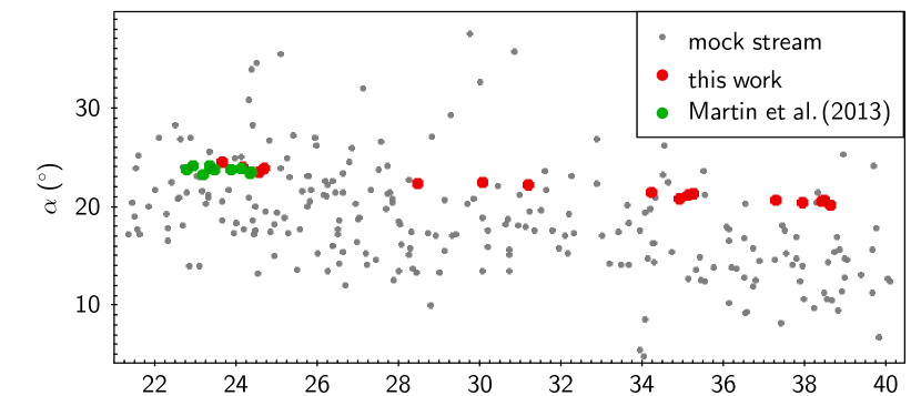
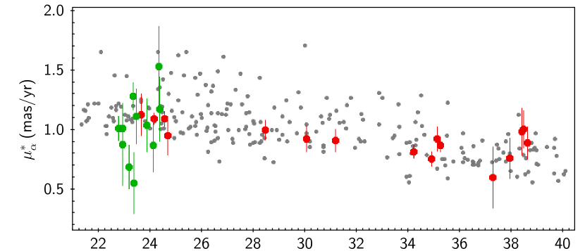
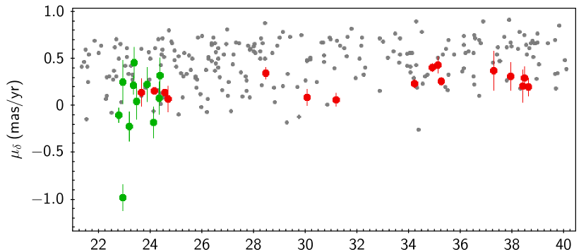
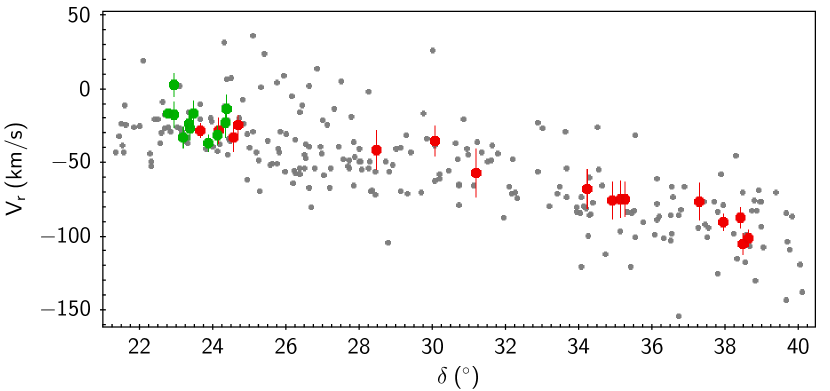
Figure 3: Right ascension $\alpha$, PMs $\mu^{*}_{\alpha}$ and $\mu_{\delta}$, and radial velocity $V_{r}$ as a function of declination $\delta$ are presented from top to bottom. The gray dots represent the stream particles within the same sky area as Triangulum. The green and red points represent the stream member stars.

3.4 Metallicity and CMD

To further examine whether Triangulum is stripped from GC NGC 5824, we compare them on the basis of metallicity and CMD.

The metallicity distribution of Triangulum members is presented in Fig. 4. There are 4 blue horizontal branch (BHB) stars and 22 red giant branch (RGB) stars. For the whole sample, the mean value $\langle\rm[Fe/H]\rangle$ = -2.10 and standard deviation $\sigma_{\rm[Fe/H]}$ = 0.26 dex are consistent with those of Martin et al. (2013) ($\langle\rm[Fe/H]\rangle$ = -2.2, $\sigma_{\rm[Fe/H]}$ = 0.3 dex). Picking out RGB stars separately is aimed for a comparison to some chemical researches on NGC 5824. Mucciarelli et al. (2018) analyzed 87 RGB stars of the cluster and obtained a metallicity distribution peaked at [Fe/H] = -2.11 dex, which is very similar to $\langle\rm[Fe/H]\rangle$ = -2.14 dex here. The observed scatter $\sigma_{\rm[Fe/H]}$ = 0.22 dex could probably be caused by observational uncertainties in low-resolution spectra ($R\sim$1800).

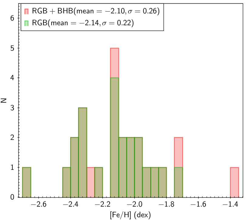
Figure 4: The metallicity distribution of Triangulum member stars. The red bars represent the whole sample and the green bars correspond to only RGB stars.

To compare Triangulum with GC NGC 5824 in CMD, we need to know the stream’s distance. Xue et al. (2011) estimated distances of $\sim$ 5000 BHB stars by matching them in ($u-g$, $g-r$) space to theoretical colors for BHB stars with a series of absolute magnitudes. The individual distances of 4 BHB stars in our sample can be obtained from this catalog: 28.8, 26.9, 30.6 and 26.0 kpc for stars with No. 4, 8, 24 and 26 in Table 1, respectively. This yields a median distance of 27.85 kpc, close to 26 kpc proposed by Bonaca et al. (2012). In addition, we also estimate distances to all 26 stars (see Fig. 10) using the method from Carlin et al. (2015), which is a Bayesian approach with likelihood estimated via comparison of spectroscopically derived atmospheric parameters to a grid of stellar isochrones, and returns a posterior probability density function for star’s absolute magnitude. This yields a median value at 33 kpc similar to 35 kpc estimated by Martin et al. (2013). We adopt the distance to Triangulum stream as $\sim$ 30 kpc, which is a median value between BHB distance and our estimate.

In CMD, we move the member stars from 30 to 32.1 kpc, where GC NGC 5824 is located (Harris 1996, 2010 edition), and find that they match well as shown in Fig. 5. The cluster stars here marked in the orange dots are obtained through sky and PM selections as instructed by Kundu et al. (2021). Specifically, we retrieve stars within the tidal radius $r_{t}$ = 5.73^′ of NGC 5824 (Harris 1996, 2010 edition) and clean the data following procedures as described in Sect. 2. A 2D Gaussian mixture model consisting of two Gaussians is then fitted in PM space to decompose the cluster and field stars apart. For the cluster component, we get the center ($\mu^{*}_{\alpha}$, $\mu_{\delta}$) = (-1.193, -2.235) with the intrinsic dispersion ($\sigma^{\rm in}_{\mu^{*}_{\alpha}}$, $\sigma^{\rm in}_{\mu_{\delta}}$) = (0.424, 0.360) mas yr^-1, where the center is very close to (-1.189, -2.234) mas yr^-1 measured by Vasiliev & Baumgardt (2021). The cluster stars are selected as those whose PMs, within uncertainties, match the PMs and dispersion of NGC 5824: $\{\mu^{*}_{\alpha}\pm\sigma_{\mu^{*}_{\alpha}},\mu_{\delta}\pm\sigma_{\mu_{\delta}}\}^{\rm star}$ $\leq$ $\{\mu^{*}_{\alpha}\pm\sigma^{\rm in}_{\mu^{*}_{\alpha}},\mu_{\delta}\pm\sigma^{\rm in}_{\mu_{\delta}}\}^{\rm cluster}$. The black line denotes the RGB locus obtained by fitting the RGB stars directly with a third-order polynomial, which is used in Sect. 4.1 to assign weights in CMD.

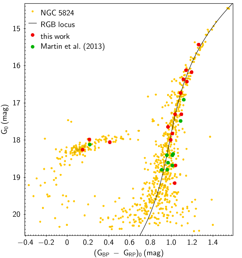
Figure 5: The orange dots represent GC NGC 5824 stars. The red and green dots represent Triangulum members. The black line denotes the RGB locus obtained by directly fitting the RGB stars with a third-order polynomial.

The connection between the stream and the cluster, based on the three aspects above, confirms that Triangulum was disrupted from GC NGC 5824. In other words, the stream can be treated as a part of the cluster’s leading tail.

4 Detecting the Trailing Tail

Motivated by the existence of leading tail for NGC 5824, in this section we aim to search for its trailing tail.

4.1 A Modified Matched Filter Method

Combining PMs and CMD together to search for extra-tidal structures of GCs has proved to be an effective way (e.g., Kundu et al. 2019a, b, 2021). Here we adopt the method from Grillmair (2019) who applied a modified matched filter technique and successfully detected a 50$\degr$ long tidal tail for GC M5.

Stars fetched in Sect. 2 are assigned weights based on their locations in CMD and PM space. In CMD, individual stars in the NGC 5824 field are assigned weights according to their color differences from the cluster locus, assuming a Gaussian error distribution:

$$w_{\rm CMD}=\frac{1}{\sqrt{2\pi}\sigma_{color}}{\rm exp}\left[-\frac{1}{2}\left(\frac{color-color_{0}}{\sigma_{color}}\right)^{2}\right].$$ (6)

Here $color$ and $\sigma_{color}$ denote $G_{BP}$ - $G_{RP}$ and corresponding errors. Color errors are simply calculated through $\sqrt{\sigma^{2}_{G_{BP}}+\sigma^{2}_{G_{RP}}}$ where $\sigma_{G_{BP}}$ and $\sigma_{G_{RP}}$ are obtained with a propagation of flux errors (see CDS website ). $color_{0}$ is determined by the cluster RGB locus (the black line in Fig. 5) at a given $G$ magnitude of a star. During assigning weights, we do not include $\sigma_{G}$ since uncertainties in $G$ band are much smaller than those in $G_{BP}$ and $G_{RP}$ (on the order of $\sim$ 0.1) for $Gaia$ photometry. Stars from $G$ = 15 mag (tip of the cluster’s RGB) to the $Gaia$ limit $G\simeq$ 21 mag are investigated.

The PMs of the model stream generated in Sect. 3.2 are further employed to weight stars. Fig. 6 shows the stream particles within the NGC 5824 field in phase space, which serves as an estimate to the real stream. In PM space, weights are computed as:

$$w_{\rm PMs}=\frac{1}{2\pi n^{2}\sigma_{\mu^{*}_{\alpha}}\sigma_{\mu_{\delta}}}{\rm exp}\left\{-\frac{1}{2}\left[\left(\frac{\mu^{*}_{\alpha}-\mu^{*}_{\alpha,0}}{n\sigma_{\mu^{*}_{\alpha}}}\right)^{2}+\left(\frac{\mu_{\delta}-\mu_{\delta,0}}{n\sigma_{\mu_{\delta}}}\right)^{2}\right]\right\}.$$ (7)

$\mu^{*}_{\alpha}$, $\mu_{\delta}$, $\sigma_{\mu^{*}_{\alpha}}$ and $\sigma_{\mu_{\delta}}$ are measured PMs and corresponding errors. $\mu^{*}_{\alpha,0}$ and $\mu_{\delta,0}$ are the components of PMs predicted at each star’s $\delta$ based on the model stream’s locus (blue lines of PM panels in Fig. 6). The locus is obtained by dividing the particles into $\delta$ bins (bin width = 1$\degr$) and calculating medians of PMs in each bin. It is worth noting that PM errors are multiplied by $n$ and we choose a moderate $n$ = 2 here, which is designed to allow some deviations between the model and observations. This can be illustrated using a one-dimensional example (see Fig. 7). Assume that we are going to assign a weight to a stream star (if exist) with $\mu_{\delta}$ = $x$ and $\sigma_{\mu_{\delta}}$ = 0.4 mas yr^-1. The $\mu_{\delta,0}$ predicted by the model stream at the star’s $\delta$ is 2 mas yr^-1. The star’s weight will be determined by a Gaussian with mean = 2 and sigma = 0.4 ($n$ = 1, red line) or 0.8 ($n$ = 2, green line). If the model predicts the stream very well, that is $x$ is very close to 2 mas yr^-1, the red line ($n$ = 1) will give a higher weight to the star apparently. However, the model stream is just an approximation to the real one and it is likely that there are small deviations between them, which might lead to that $x$ falls out of the blue dashed lines. When this happens, the green line ($n$ = 2) gives a higher weight. We have compared results using different $n$ values and verified that $n$ = 2 is the most favorable.

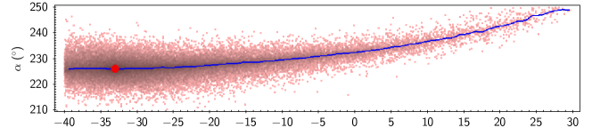
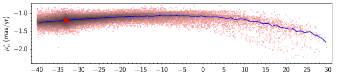
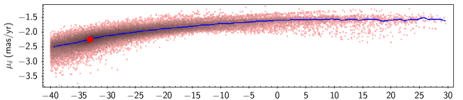
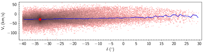
Figure 6: The planes of $\alpha$, heliocentric distance, proper motion in $\alpha$ and $\delta$, and radial velocity as a function of $\delta$, are shown from the top to the bottom, respectively. The pink dots represent the model stream particles within the NGC 5824 field. The red circle represents GC NGC 5824. The blue lines denote medians of y-axis values in each $\delta$ bin with a bin width of 1$\degr$.

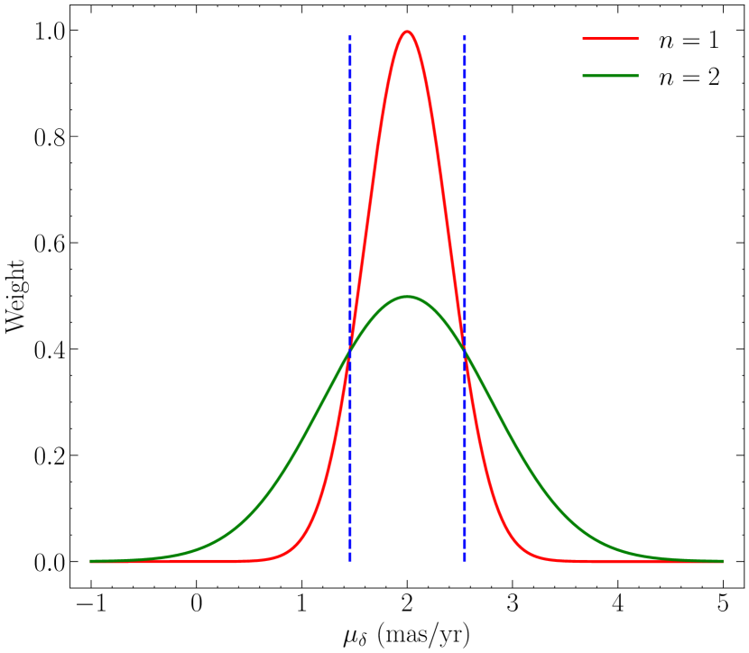
Figure 7: Illustration for using $n$ = 2 in Eq. (7). The red and green lines represent Gaussians centered at 2 with sigma = 0.4 and 0.8 mas yr^-1, respectively.

Finally, stars weights are obtained by multiplying $w_{\rm CMD}$ and $w_{\rm PMs}$, and then summed in $0.2\degr\times 0.2\degr$ sky pixels to expose structures.

4.2 Results

A weighted sky map is obtained after applying the above method to data in the cluster field and shown in the left panel of Fig. 8. To make the stream look more prominent, pixels with summed weights $>$ 80 and $<$ 2 are masked such that too strong noises and weak background are not shown. The map is then smoothed with a Gaussian kernel of $\sigma$ = 0.5$\degr$. The stretch is logarithmic, with brighter areas corresponding to higher weight regions. The blue circle on the bottom marks the location of NGC 5824. The white bottom-right corner is due to being close to the Galactic disk, which is further masked in the middle and right panels.

Figure 8: Log stretch of a matched filter map in the NGC 5824 field. The sky pixel width is 0.2$\degr$ and the map is smoothed with a Gaussian kernel of $\sigma$ = 0.5$\degr$. Three panels present the same map. The white arrows in left panel point the stream features. The locus of the model stream is overplotted in the small red dots in middle panel. The right panel illustrates the way of creating the stream’s lateral profile (see text). Bottom-right region close to the Galactic disk is masked in the middle and right panels.

Due to the photometric depth of $Gaia$, the cluster’s main sequence stars are not observable and only RGB stars can be used to trace the underlying trailing tail, which are much fewer than the former. However, some stream-like signals are still detected. In the left panel, it is clear that there are several structures (marked with arrows) with higher weights between $\delta\simeq$ -21 $-$ -4$\degr$ that could be connected smoothly and likely extended from NGC 5824. In the middle panel, we overplot the trajectory of the model stream (small red dots) and find that it passes through the structures well. An additional segment of $\delta\simeq$ 6 $-$ 16$\degr$ is a farther extension of the stream. There is a gap in the middle at $\delta\simeq$ -4 $-$ 6$\degr$ corresponding to the most distant range of the model stream (see the distance panel in Fig. 6), where many RGB stars might have been darker than 21 mag. The detected signature traces the cluster’s trailing tail to $\sim 50\degr$ whose path can be roughly fitted using

$$\alpha=4.07\times 10^{-5}\delta^{3}+6.68\times 10^{-3}\delta^{2}+0.37\delta+232.45$$ (8)

where -33$\degr$ $<$ $\delta$ $<$ 16$\degr$.

In the right panel of Fig. 8, stars enclosed by the red lines are selected to calculate the statistical significance of the stream. The $\delta$ range is $-22\degr--3\degr$. The central dashed line represents a more precise description to the stream of this region, which is given by

$$\alpha=7.15\times 10^{-3}\delta^{2}+0.38\delta+232.58+{\rm offset}$$ (9)

with offset = 0$\degr$. The left and right boundaries correspond to offset = -4 and 4$\degr$, respectively. A bin width = 0.2$\degr$ is used and at offset = -4, -3.8, -3.6…, weights of stars around Eq. (9) $\pm 0.1\degr$ are integrated to create a lateral profile of the stream as displayed in Fig. 9. The central peak at offset = 0$\degr$ represents the stream feature. The larger random counts at positive side are caused by higher stellar density near the disk. The significance is defined as $S=(w_{stream}-w_{background})/\sigma_{background}$, where $w_{stream}$ is the stream signal and $w_{background}$ and $\sigma_{background}$ are the mean and standard deviation of weights for off-stream regions 0.5$\degr$ $<$ —offset— $<$ 4$\degr$. We get S = 7.5 and 3.6 for negative and positive sides, respectively, and S is 4.3 if both are considered. It can be inferred from Fig. 9 that the stream’s width is expected to be $\lesssim 0.2\degr$ because signals drop back to the level of background when —offset— $>$ 0.1$\degr$ which means that there are few stream signals beyond this range. If we adopt $d$ = 39 kpc for this segment based on the model, the physical width is $\lesssim$ 136 pc.

Figure 9: The stream one-dimensional profile. The offset coordinate is defined as deviation from the stream along $\alpha$ direction (see Eq. (9)).

4.3 A Part of Cetus?

Bonaca et al. (2021) pointed that GC NGC 5824 and Cetus (Newberg et al. 2009), which is a stellar stream with a dwarf galaxy origin, have very close orbital energies and angular momenta. Similar orbital trajectories between them are also demonstrated in Chang et al. (2020). This arises a question: do those features on the trailing side of the cluster belong to Cetus stream?

Combining the results here with previous researches on Cetus, we present 4 reasons for that the detected features are indeed related to the trailing tail of NGC 5824.

1. The width of features in Fig. 8 is only $\lesssim 0.2\degr$, which is thin compared to a stream produced by a dwarf galaxy.

2. Cetus stars should have a relatively spread distribution in CMD. However, the stream features indicated with arrows in Fig. 8 disappear if the RGB locus used to weight stars in CMD is shifted either blueward or redward by 0.1 mag, which means that they are exactly corresponding to NGC 5824.

3. Chang et al. (2020) pointed that GC NGC 5824 should not be the core of Cetus, implying that there is no direct connection between the cluster and Cetus stream. Furthermore, Yuan et al. (2021) concentrated on searching for Cetus’s members using data covering the cluster but they did not detect any densely populated structure around NGC 5824. Hence the features should not be a part of Cetus.

4. Triangulum as a piece of the leading tail also provides a weak evidence of existence for the trailing tail.

5 Discussion

During comparing Triangulum to the model stream in distance, we find some incompatibility and show them in Fig. 10. Bonaca et al. (2012) estimated a Triangulum’s distance of 26 $\pm$ 4 kpc (the lower black error bar) while Martin et al. (2013) proposed 35 $\pm$ 3 kpc (the upper black error bar) for the stream. As mentioned above, we adopt a distance of 30 kpc (the green solid line) and find that the member stars match with GC NGC 5824 well in CMD. However, under a static Milky Way potential plus a moving LMC, the resulting model stream predicts that Triangulum’s distance should be about 20 - 25 kpc (gray dots), which is true in both this work and Li et al. (2022) (the second panel of Fig. 8 therein). This arises a confusion: why is there such a difference?

Figure 10: Heliocentric distance as a function of $\delta$. The gray dots represent the stream particles. The blue points represent 4 BHB stars in our samples, whose distances come from Xue et al. (2011). The red dots and error bars present distances and corresponding errors for all member stars estimated using the method of Carlin et al. (2015). The red dashed line corresponds to their median value 33 kpc. The green solid line marks adopted distance 30 kpc. Two black error bars represent 26 $\pm$ 4 kpc (Bonaca et al. 2012) and 35 $\pm$ 3 kpc (Martin et al. 2013).

Sheffield et al. (2014) presented an analysis on TriAnd1 ($d\sim$ 20 kpc) and TriAnd2 ($d\sim$ 28 kpc) (Martin et al. 2007), other two stellar substructures in the direction of M31 and M33. They show that even though the two structures are separated by more than 5 kpc in distance, they are indistinguishable in radial velocity and PMs. We note that this kinematic feature is very similar to that of Triangulum when compared to the model stream. The real and mock streams are separated by more than 5 kpc as well but their trends in phase space are still in concordance. Considering that the stream and those structures are exactly in the same region, it is very likely that Triangulum has been affected by the mechanism which leads to TriAnd1 and TriAnd2. Specifically, either related to a dwarf galaxy (Sheffield et al. 2014) or the Galactic disk (Xu et al. 2015), some process that created TriAnd1 and TriAnd2 might push Triangulum farther away (30 kpc) from where it should be (20 - 25 kpc). We anticipate that this prediction could be proved by later simulations on the formation of TriAnd overdensities.

It is also worth nothing that there is another stream segment named Turbio (Shipp et al. 2018) between Triangulum and GC NGC 5824 that was considered to be disrupted from the cluster based on their similar dynamics in Bonaca et al. (2021) and Li et al. (2022). We do not inspect this stream due to lack of spectroscopic data. It is expected that upcoming observations will be able to provide more details on connections between Turbio and the cluster, and even more opportunities of searching for other stream segments on the leading side. If these can be confirmed, NGC 5824 tidal tails would be the longest cold stream ever discovered in the Milky Way.

6 Conclusions

We first validate the connection between Triangulum stream and NGC 5824. A total of 26 stream member stars are selected and 16 of them are newly identified. We model the cluster’s disruption under a static Milky Way potential accompanied with a moving LMC. The real stream is compared to the mock one in phase space and consistent trends can be found. In metallicity and CMD, the member stars and the cluster are also in good agreement. These results support the previous statement that Triangulum originates from GC NGC 5824 (Bonaca et al. 2021; Li et al. 2022).

Given that Triangulum can be considered as a segment of the cluster’s leading tail, we examine the existence of its trailing tail. Using a matched-filer method that combines CMD and PMs to weight stars, we find a $\sim$ 50$\degr$ trailing tail for GC NGC 5824. The features match with the model stream well. Although the signals are tenuous and discrete, a peak of $>$ 3$\sigma$ over background noises can be still discerned in the lateral stream profile, from which we estimate that its width is $\lesssim$ 0.2$\degr$. We expect that follow-up observations will be able to provide more details about the NGC 5824 stream.