Probing high scale seesaw and PBH generated dark matter via gravitational waves with multiple tilts

Abstract

We propose a scenario where a high scale seesaw origin of light neutrino mass and gravitational dark matter (DM) in MeV-TeV ballpark originating from primordial black hole (PBH) evaporation can be simultaneously probed by future observations of stochastic gravitational wave (GW) background with multiple tilts or spectral breaks. A high scale breaking of an Abelian gauge symmetry ensures the dynamical origin of seesaw scale while also leading to formation of cosmic strings responsible for generating stochastic GW background. The requirement of correct DM relic in this ballpark necessitates the inclusion of a diluter as PBH typically leads to DM overproduction. This leads to a second early matter dominated epoch after PBH evaporation due to the long-lived diluter. These two early matter dominated epochs, crucially connected to the DM relic, leads to multiple spectral breaks in the otherwise scale-invariant GW spectrum formed by cosmic strings. We find interesting correlations between DM mass and turning point frequencies of GW spectrum which are within reach of several near future experiments like LISA, BBO, ET, CE etc.

I Introduction

The observation of neutrino oscillation has been the most compelling experimental evidence suggesting the presence of beyond standard model (BSM) physics. This is because the standard model (SM) alone can not explain the origin of neutrino mass and mixing, as verified at neutrino oscillation experiments Zyla:2020zbs ; Mohapatra:2005wg . Different BSM frameworks have, therefore, been invoked to explain non-zero neutrino mass as in the SM, there is no way to couple the left handed neutrinos to the Higgs field in the renormalisable Lagrangian due to the absence of right chiral neutrinos. Conventional neutrino mass models based on seesaw mechanism Minkowski:1977sc ; GellMann:1980vs ; Mohapatra:1979ia ; Schechter:1980gr ; Mohapatra:1980yp ; Lazarides:1980nt ; Wetterich:1981bx ; Schechter:1981cv ; Foot:1988aq typically involve introduction of heavy fields like right handed neutrinos (RHN). Typically, such canonical seesaw models have a very high seesaw scale keeping it away from the reach of any direct experimental test. This has led to some recent attempts in finding ways to probe high scale seesaw via stochastic gravitational wave (GW) observations Dror:2019syi ; Blasi:2020wpy ; Fornal:2020esl ; Samanta:2020cdk ; Barman:2022yos ; Huang:2022vkf ; Dasgupta:2022isg ; Okada:2018xdh ; Hasegawa:2019amx ; Borah:2022cdx . These scenarios consider the presence of additional symmetries whose spontaneous breaking not only lead to the dynamical generation of RHN masses but also lead to generation of stochastic GW from topological defects like cosmic strings Dror:2019syi ; Blasi:2020wpy ; Fornal:2020esl ; Samanta:2020cdk , domain walls Barman:2022yos or from bubbles generated at first order phase transition Huang:2022vkf ; Dasgupta:2022isg ; Okada:2018xdh ; Hasegawa:2019amx ; Borah:2022cdx .

In addition to the origin of neutrino mass, the SM also fails to explain the origin of dark matter (DM), a mysterious, non-luminous and non-baryonic form of matter comprising around $27\%$ of the present universe. The present DM abundance is often reported in terms of density parameter $\Omega_{\rm DM}$ and reduced Hubble constant $h=\text{Hubble Parameter}/(100\;\text{km}~{}\text{s}^{-1}\text{Mpc}^{-1})$ as Aghanim:2018eyx

$$\Omega_{\text{DM}}h^{2}=0.120\pm 0.001$$ (1)

at 68% CL. Among a variety of BSM proposals to explain the origin of DM, the weakly interacting massive particle (WIMP) has been the most well-studied one. In WIMP framework, a particle having mass and interactions around the electroweak ballpark can lead to the observed DM abundance after undergoing thermal freeze-out in the early universe Kolb:1990vq . While WIMP has promising direct detection signatures, contrary to high scale seesaw, the null results at direct detection experiments LUX-ZEPLIN:2022qhg have motivated to consider other alternatives. Such alternative DM scenarios may have suppressed direct detection signatures but can leave signatures at future GW experiments. There have been several recent works on such GW signatures of DM scenarios Yuan:2021ebu ; Tsukada:2020lgt ; Chatrchyan:2020pzh ; Bian:2021vmi ; Samanta:2021mdm ; Borah:2022byb ; Azatov:2021ifm ; Azatov:2022tii ; Baldes:2022oev .

Motivated by this, we consider a high scale seesaw scenario with gravitational DM generated from evaporating primordial black holes (PBH) assuming the latter to dominate the energy density of the universe at some stage. While the seesaw scale is dynamically generated due to spontaneous breaking of a $U(1)$ gauge symmetry at high scale, DM can be generated during a PBH dominated epoch. Unlike superheavy DM considered in most of the PBH generated DM scenarios, we consider DM around MeV-TeV ballpark Barman:2022gjo . Since DM in this ballpark gets overproduced during a PBH dominated era, we also consider the presence of a long-lived diluter whose late decay brings the DM abundance within limits. The diluter is also dominantly produced from PBH as its coupling with the SM remains suppressed in order to keep it long-lived. The high scale breaking of $U(1)$ gauge symmetry leads to the formation of cosmic strings (CS) Kibble:1976sj ; Nielsen:1973cs , which generate stochastic GW background with a characteristic spectrum within the reach of near future GW detectors if the scale of symmetry breaking is sufficiently high Vilenkin:1981bx ; Turok:1984cn . In the present setup we show that the PBH domination followed by subsequent diluter domination era lead to multiple spectral breaks in the GW spectrum formed by CS network. In a recent work Borah:2022byb the correlation between such spectral break due to non-standard cosmological era Cui:2017ufi ; Cui:2018rwi ; Gouttenoire:2019kij of diluter domination and DM properties was studied within the framework of a realistic particle physics model with high scale seesaw. Here we extend this to a PBH generated gravitational DM scenario with the unique feature of multiple spectral breaks in scale-invariant GW background generated by CS, not considered in earlier works. Depending upon DM mass, the three spectral breaks or turning point frequencies can be within reach of different future GW experiments.

This paper is organised as follows. In section II, we briefly discuss our setup followed by discussion of dark matter relic from PBH in section III. In section IV, we discuss the details of gravitational wave spectrum generated by cosmic strings and subsequent spectral breaks due to PBH and diluter domination for different DM masses. Finally, we conclude in section V.

II The Framework

The present framework can be embedded in any Abelian extension of the SM that guarantees the formation of cosmic strings due to the spontaneous symmetry breaking with an era of primordial black hole domination. A singlet scalar with no coupling to the SM or the new Abelian gauge sector is assumed to be the DM having purely gravitational interactions. A diluter in the form of a heavy singlet Majorana fermion or a heavy RHN is also incorporated while keeping its coupling to the SM leptons tiny. In order to ensure that the PBH domination and diluter domination arise as separate epochs for simplicity, we consider the diluter to be singlet under the new Abelian gauge symmetry as well.

For a demonstrative purpose, here we consider an anomaly free $U(1)_{L_{\mu}-L_{\tau}}$ extension of the SM gauge symmetry where $L_{\mu}$ and $L_{\tau}$ represent the muon and tau lepton numbers respectively He:1990pn ; He:1991qd . The SM particle content is extended with three additional right-handed neutrinos ($N^{e}_{R},N^{\mu}_{R},N^{\tau}_{R}$) and a complex scalar ($S$) that is a singlet under the SM gauge symmetry but carries $1$ unit of $U(1)_{L_{\mu}-L_{\tau}}$ charge. As the symmetry suggests, the muon and tau takes $1$ and $-1$ unit of charge under the $U(1)_{L_{\mu}-L_{\tau}}$ respectively. The newly introduced RHNs are singlets under the SM gauge symmetry, while two carry 1 and $-1$ unit of $U(1)_{L_{\mu}-L_{\tau}}$ charges and the third remains uncharged.

Next, we write all the possible interactions the different particles can have in the present setup. The kinetic terms for the additional fields read as,

$$\mathcal{L^{KE}} =\frac{i}{2}\sum_{\alpha=e,\mu,\tau}N_{\alpha}\gamma^{\delta}D_{\delta}N_{\alpha}+(D^{\delta}S)^{\dagger}(D_{\delta}S)$$ (2)

where $D_{\delta}=\partial_{\delta}+ig_{\mu\tau}Q_{\mu\tau}(Z_{\mu\tau})_{\delta}$ with $Q_{\mu\tau}$ representing the charge and $Z_{\mu\tau}$ being the gauge boson of $U(1)_{L_{\mu}-L_{\tau}}$ symmetry. The Lagrangian involving the Yukawa interactions and masses of the additional fermions involved can be written as,

$$\mathcal{L}= -\frac{1}{2}h_{e\mu}(\bar{N}^{c}_{e}N_{\mu}+\bar{N}^{c}_{\mu}N_{e})S^{\dagger}-\frac{1}{2}h_{e\tau}(\bar{N}^{c}_{e}N_{\tau}+\bar{N}^{c}_{\tau}N_{e})S-\sum_{\alpha=e,\mu,\tau}Y_{\alpha}\bar{L}_{\alpha}\tilde{H}N_{\alpha}$$

$$-\frac{1}{2}M_{ee}\bar{N}^{c}_{e}N_{e}-\frac{1}{2}M_{\mu\tau}(\bar{N}^{c}_{\mu}N_{\tau}+\bar{N}^{c}_{\tau}N_{\mu})S+h.c.$$ (3)

The most general scalar potential involving the different scalars can be expressed as,

$$V(H,S)= -\mu^{2}_{H}H^{\dagger}H-\mu^{2}_{S}S^{\dagger}S+\lambda_{H}(H^{\dagger}H)^{2}+\lambda_{S}(S^{\dagger}S)^{2}+\lambda_{HS}(H^{\dagger}H)(S^{\dagger}S).$$ (4)

The scalar $S$ breaks the $U(1)_{L_{\mu}-L_{\tau}}$ symmetry once its CP even component develops a non-zero vacuum expectation value (vev) $v_{\mu\tau}$. This breaking also results in an additional non-zero mixing between the RHNs as can be seen from Eq. (3). Once the Electroweak Symmetry is broken, the Higgs doublet ($H$) also develops a non-zero vev $v=246$ GeV. As a result of electroweak symmetry breaking, the different scalars will mix with each other. We will not go into the details of the scalar mixing as it remains unimportant for our analysis and refer the reader to Asai:2017ryy for the details. In fact, due to the restrictive nature of Dirac neutrino and RHN mass matrices, fitting light neutrino data requires another singlet scalar, as pointed out in Asai:2017ryy ; Borah:2021mri . The details of these extensions does not affect our analysis and hence we skip it here.

Finally, we consider scalar singlet dark matter $\phi$ to have only gravitational interactions and hence it has a bare mass term (denoted by $M_{\text{DM}}$) only in the Lagrangian. Another heavy RHN, similar to $N^{e}$ with vanishing $U(1)_{L_{\mu}-L_{\tau}}$ charge but tiny couplings to leptons is considered to be negligible. This diluter RHN, to be denoted as $N_{3}$, also couples more feebly to other RHNs so that $N_{3}$ dominantly decays into $L_{e},H$ at late epochs. While $N_{e}$ could, in principle, play the role of diluter as well, it will lead to difficulties in generating correct light neutrino data due to restricted mass matrix structures. Due to tiny couplings of $N_{3}$ with other particles in thermal bath, it is produced only non-thermally from the evaporation of the PBH. The consequence of this slow decay is a $N_{3}$ dominated epoch after the evaporation of PBH, as we discuss below.

III Dark matter and diluter from PBH

As mentioned above, the DM in the present framework only has gravitational interactions and hence can be dominantly produced from PBH evaporation. On the other hand, as a result of its feeble interaction with the SM bath, $N_{3}$ can also be assumed to be produced purely from the PBH evaporation. While the PBH itself can act as a DM if its mass is chosen appropriately, in this work we focus in the ultra-light mass regime of PBH where it is not cosmologically long-lived. As is well known from several earlier works, the DM in a mass range: few keV to around $10^{10}$ GeV, when produced from the PBH evaporation are always overabundant Fujita:2014hha ; Samanta:2021mdm and can overclose the energy density of the universe. A recent study Barman:2022gjo has shown that the overproduction of such DM can be prevented if one considers a diluter that injects entropy at a late time into the thermal bath as a result of its slow decay. Following Barman:2022gjo , in the present work we also consider such multiple early matter-dominated eras and show how their presence can affect the GW spectrum generated by cosmic strings in a unique way.

PBH is assumed to be formed in the era of radiation domination after inflation. In such a situation, the PBH abundance is characterized by a dimensionless parameter $\beta$ defined as

$$\beta=\frac{\rho_{\text{BH}}(T_{\text{in}})}{\rho_{\text{R}}(T_{\text{in}})},$$ (5)

where $\rho_{\text{BH}}(T_{\text{in}})$ and $\rho_{\text{R}}(T_{\text{in}})$ represents the initial PBH energy density and radiation energy density respectively while $T_{\text{in}}$ denotes the temperature at the time of PBH formation. The expression of $T_{\text{in}}$ can be found in appendix A. Once PBHs are formed, the radiation-dominated universe eventually turns into a matter-dominated universe and remains matter-dominated till the epoch of PBH evaporation. The temperature corresponding to the PBH evaporation is denoted as $T_{\text{ev}}$ and can be obtained from Eq. (30). The condition determining PBH’s evaporation during the radiation-domination is given as Masina:2020xhk ,

$$\beta<\beta_{\text{c}}\equiv\gamma^{-1/2}\,\sqrt{\frac{\mathcal{G}\,g_{\star}(T_{\text{BH}})}{10640\,\pi}}\,\frac{M_{\text{pl}}}{m_{\text{in}}}\,,$$ (6)

where $\beta_{c}$ is the critical PBH abundance that leads to an early matter-dominated era. In our scenario, we consider $\beta$ to be large enough such that PBH dominate the energy density of the universe at some epoch. In the above inequality, $\gamma\simeq 0.2$ is a numerical factor that contains the uncertainty of the PBH formation and $\mathcal{G}\sim 4$ is the grey-body factor. Here, $M_{\text{pl}}$ denotes the Planck mass while $m_{\text{in}}$ and $T_{\text{BH}}$ denote the mass of PBH at the time of formation and instantaneous Hawking temperature of PBH (see appendix A for the details). Additionally, we also assume the PBHs to be of Schwarzschild type without any spin and charge and having a monochromatic mass spectrum implying all PBH to have identical masses. It is important to mention that a PBH can dominantly evaporate only into particles lighter than its instantaneous Hawking temperature.

An upper bound on the PBH mass is obtained by demanding its evaporation temperature $T_{\text{ev}}>T_{\text{BBN}}\simeq 4$ MeV, as the evaporation of PBH also results in the production of the radiation that can disturb the successful prediction of the big bang nucleosynthesis (BBN). While the upper bound on the PBH mass can be obtained by comparing its evaporation temperature with the BBN temperature, a lower bound on its mass can be obtained from the cosmic microwave background (CMB) bound on the scale of inflation, $i.e.$ $\mathcal{H}_{I}\equiv\mathcal{H}(T_{\text{in}})\leq 2.5\times 10^{-5}\,M_{\text{pl}}$, where $\mathcal{H}(T_{\text{in}})=\frac{1}{2\,t_{\text{in}}}$ with $t(T_{\text{in}})=\frac{m_{\text{in}}}{M_{\text{pl}}^{2}\,\gamma}$ (as obtained from Eq. (23)). Using these BBN and CMB bounds together, we have a window for allowed initial mass for PBH that reads $0.1\,\text{g}\lesssim m_{\text{in}}\lesssim 3.4\times 10^{8}\,\text{g}$. The range of PBH masses between these bounds is at present generically unconstrained Carr:2020gox . It should be noted that the upper bound is obtained only for PBH which evaporate on a timescale smaller than the age of the universe and have a large initial fraction $\beta$ to dominate the energy density at some epoch.

III.1 Particle production from PBH

Once formed, the PBH can evaporate by Hawking radiation Hawking:1974rv ; Hawking:1975vcx . Among the products of PBH evaporation, there might be a stable BSM particle that can contribute to the observed DM abundance Morrison:2018xla ; Gondolo:2020uqv ; Bernal:2020bjf ; Green:1999yh ; Khlopov:2004tn ; Dai:2009hx ; Allahverdi:2017sks ; Lennon:2017tqq ; Hooper:2019gtx ; Chaudhuri:2020wjo ; Masina:2020xhk ; Baldes:2020nuv ; Bernal:2020ili ; Bernal:2020kse ; Lacki:2010zf ; Boucenna:2017ghj ; Adamek:2019gns ; Carr:2020mqm ; Masina:2021zpu ; Bernal:2021bbv ; Bernal:2021yyb ; Samanta:2021mdm ; Sandick:2021gew ; Cheek:2021cfe ; Cheek:2021odj ; Barman:2022gjo or there might be a new particle produced which is responsible for generating the present matter-antimatter asymmetry of the universe Hawking:1974rv ; Carr:1976zz ; Baumann:2007yr ; Hook:2014mla ; Fujita:2014hha ; Hamada:2016jnq ; Morrison:2018xla ; Hooper:2020otu ; Perez-Gonzalez:2020vnz ; Datta:2020bht ; JyotiDas:2021shi ; Smyth:2021lkn ; Barman:2021ost ; Bernal:2022pue ; Ambrosone:2021lsx ; Barman:2022gjo ; Bhaumik:2022pil . The number of any particle $X$ produced during the evaporation of a single PBH is given by

$$\mathcal{N}_{X}=\frac{g_{X,H}}{g_{\star,H}(T_{\text{BH}})}\begin{cases}\frac{4\,\pi}{3}\,\Bigl{(}\frac{m_{\text{in}}}{M_{\text{pl}}}\Bigr{)}^{2}&\text{for }m_{X}<T_{\text{BH}}^{\text{in}}\,,\\[8.0pt] \frac{1}{48\,\pi}\,\Bigl{(}\frac{M_{\text{pl}}}{m}\Bigr{)}^{2}&\text{for }m_{X}>T_{\text{BH}}^{\text{in}}\,,\end{cases}\,,$$ (7)

where

$${g_{X,H}}(T_{\text{BH}})\equiv\sum_{i}\omega_{i}\,g_{i,H}\,;g_{i,H}=\begin{cases}1.82&\text{for }s=0\,,\\ 1.0&\text{for }s=1/2\,,\\ 0.41&\text{for }s=1\,,\\ 0.05&\text{for }s=2\,,\\ \end{cases}$$ (8)

with $\omega_{i}=2\,s_{i}+1$ for massive particles of spin $s_{i}$, $\omega_{i}=2$ for massless species with $s_{i}>0$ and $\omega_{i}=1$ for $s_{i}=0$. Here, $T_{\text{BH}}^{\text{in}}$ denotes the instantaneous PBH temperature at the time of the formation. The yield of a particle produced during the evaporation of a PBH is related to the PBH abundance ($n_{\text{BH}}$) and is expressed as,

$$Y_{\mathcal{N}_{X}}(T_{0})=\frac{n_{\mathcal{N}_{X}}}{s}\bigg{|}_{T_{0}}=\mathcal{N}_{X}\frac{n_{\text{BH}}}{s}\bigg{|}_{T_{\text{ev}}}.$$ (9)

PBH abundance at the time of its evaporation can be obtained using the first Friedmann equation as

$$n_{\text{BH}}(T_{\text{ev}})=\frac{1}{6\,\pi}\,\frac{M_{\text{pl}}^{2}}{m_{\text{in}}^{2}\,\tau^{2}}\equiv\frac{1}{6\,\pi}\,\left(\frac{\mathcal{G}\,g_{\star,H}}{10640\,\pi}\right)^{2}\,\frac{M_{\text{pl}}^{10}}{m_{\text{in}}^{7}}\,.$$ (10)

Substituting Eq. (10) in Eq. (9), one can easily obtain the asymptotic yield of the particles produced during the PBH evaporation.

Following this, one can easily calculate the abundance of the DM and the diluter ($N_{3}$) produced during the evaporation of the PBH. Once the number of DM particles produced from PBH evaporation is known, the DM relic abundance $\Omega_{\text{DM}}h^{2}$ at the present epoch can be calculated as

$$\Omega_{\text{DM}}\,h^{2}=\mathbb{C}(T_{\text{ev}})\begin{cases}\frac{1}{\pi^{2}}\,\sqrt{\frac{M_{\text{pl}}}{m_{\text{in}}}}\,m_{\text{DM}}&\text{for }m_{\text{DM}}<T_{\text{BH}}^{\text{in}}\,,\\ \frac{1}{64\,\pi^{4}}\left(\frac{M_{\text{pl}}}{m_{\text{in}}}\right)^{5/2}\,\frac{M_{\text{pl}}^{2}}{m_{\text{DM}}}&\text{for}~{}m_{\text{DM}}>T_{\text{BH}}^{\text{in}},\end{cases}\,$$ (11)

with $\mathbb{C}(T_{\text{ev}})=\frac{s_{0}}{\rho_{c}}\,\frac{1}{\zeta}\,\frac{g_{X,H}}{g_{\star,H}}\,\frac{5}{g_{\star s}(T_{\text{ev}})}\,\,\left(\frac{\pi^{3}\,g_{\star}(T_{\text{ev}})}{5}\right)^{3/4}\,\sqrt{\frac{\mathcal{G}\,g_{\star,H}}{10640\,\pi}}$. Here $\zeta$ parametrizes a possible entropy production after PBH evaporation until now, i.e., $\zeta\,\left(sa^{3}\right)_{\text{evap}}=\left(sa^{3}\right)_{0}$. Looking at the above equation one finds that the heavier the DM mass (for $m_{\text{DM}}>T_{\text{BH}}^{\text{in}}$), the lesser will be the DM relic abundance. On contrary, in a scenario with $m_{\text{DM}}<T_{\text{BH}}^{\text{in}}$, the DM relic abundance becomes proportional to the DM mass. The parameter space for DM produced during the PBH evaporation is highly constrained. The correct relic abundance is satisfied only if $m_{\text{DM}}\gtrsim 10^{10}$ GeV and $m_{\text{in}}\gtrsim 10^{6}$g Fujita:2014hha ; Samanta:2021mdm . In the rest of the parameter space, the DM is mostly overabundant if one assumes that there exists no entropy injection into the thermal plasma after the evaporation of the PBH, $i.e.~{}\zeta=1$. This tension can be relaxed considerably if one assumes $\zeta\sim\mathcal{O}(10)~{}\text{or}~{}\mathcal{O}(100)$. While DM of mass around keV or lighter do not get overproduced, it suffers from strong Lyman-$\alpha$ bounds Diamanti:2017xfo ; Bernal:2020bjf severely restricting the parameter space in $\beta-m_{\rm in}$ plane. We do not consider such light or superheavy DM in our setup and focus on the intermediate mass range which typically gets overproduced during a PBH dominated phase.

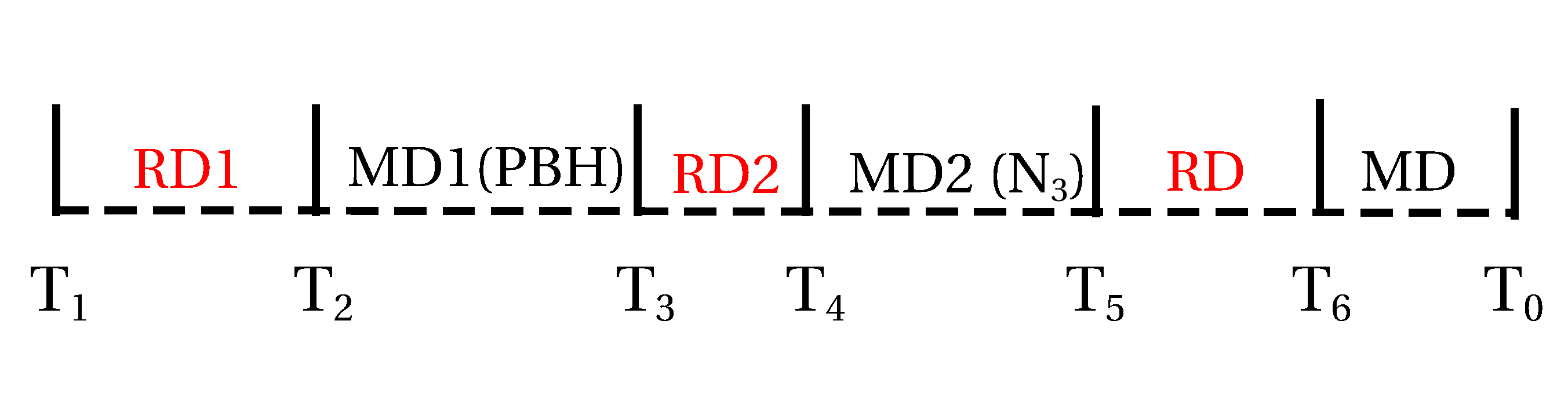
Figure 1: A schematic of the dominant phases of evolution of the universe at different epochs from a reheating temperature $T_{1}$ to the present temperature $T_{0}$ (neglecting recent dark energy domination). $T_{3}$ is the black hole evaporation temperature (equation (30)) and $T_{6}$ represents the standard matter-radiation equality temperature of $\sim 0.75$ eV.

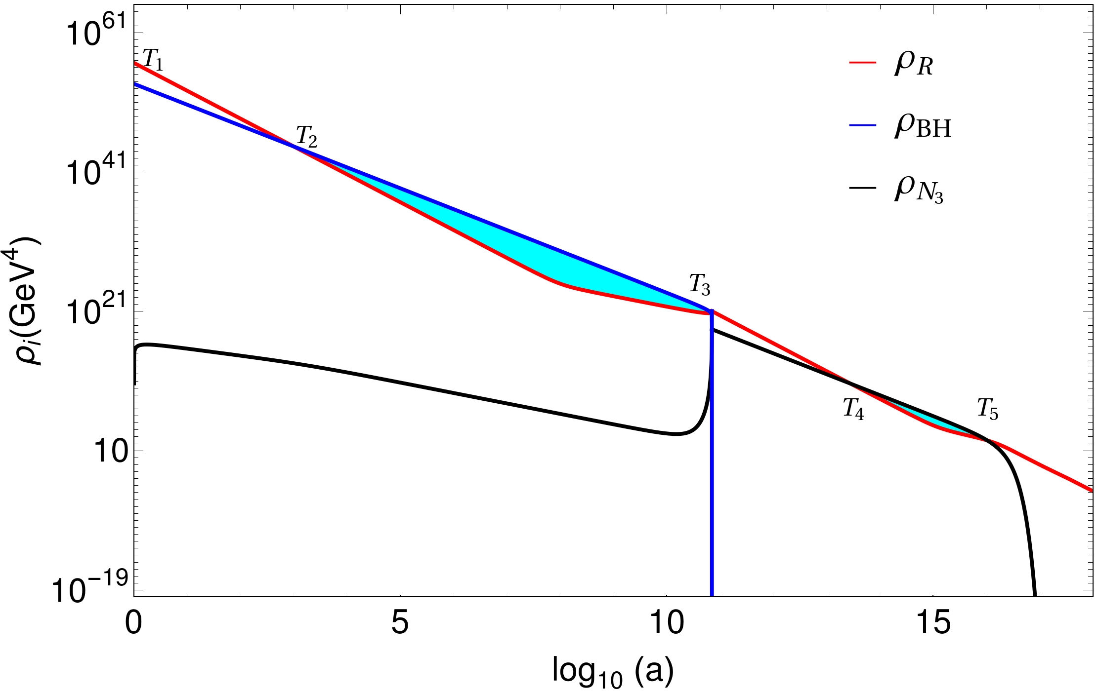
Figure 2: Evolution of the energy densities of different components in the universe clearly showing the two intermediate early matter-dominated phases due to PBH and diluter $N_{3}$ respectively. $a$ represents the scale factor with the initial value $a_{\rm in}=1$. Here, we take $m_{\rm in}=5000$ g, $M_{\rm DM}=0.1$ GeV, $M_{3}=10^{11}$ GeV.

Analogous to the DM, the diluter $N_{3}$ is also produced during the PBH’s evaporation whose abundance can be calculated using Eq. (9). Once produced, it decays very slowly as a result of its very feeble interaction with the first generation of the SM lepton doublet and the Higgs. Subsequent to the PBH evaporation, the universe enters into a radiation-dominated era for a short duration following which the energy density of $N_{3}$ overtakes the radiation energy density and the universe re-enters the matter-dominated phase in a similar manner as was shown in Barman:2022gjo . The universe experiences a rise in temperature as the diluter starts to decay. This is because, in the process of its decay, the diluter also injects entropy into the thermal bath. Finally, after the decay of the $N_{3}$ is complete the universe again becomes radiation-dominated. A schematic of the scenario is shown in Fig. 1 and the evolution of the energy densities of the different components is shown in Fig. 2 for a particular choice of benchmark parameters. As a result of the entropy injection, the number density of DM is brought within observed limits thereby alleviating the tension of DM relic abundance produced from PBH evaporation in the intermediate mass range mentioned before.

It should be noted that in addition to PBH evaporation, DM and diluter can also be produced from $2$ to $2$ scatterings mediated by massless graviton. Adopting the approach discussed in earlier works Barman:2022gjo ; Garny:2015sjg ; Tang:2017hvq ; Garny:2017kha ; Bernal:2018qlk ; Barman:2021ugy ; Bernal:2021yyb , we find that such productions are negligible for the choices of $m_{\rm in},M_{\rm DM}$ and $N_{3}$ mass $M_{3}$ considered in our numerical analysis to be discussed below.

IV Gravitational Waves from Cosmic Strings

Cosmic strings Kibble:1976sj ; Nielsen:1973cs , are one-dimensional objects which appear as topological defects after the spontaneous breaking of a symmetry group containing a vacuum manifold that is not simply connected Nielsen:1973cs . The simplest group that exhibits such feature is $U(1)$ which naturally appears in many BSM frameworks. Numerical simulations Ringeval:2005kr ; Blanco-Pillado:2011egf based on Nambu-Goto action indicate that dominant energy loss from a string loop is in the form of GW radiation if the underlying symmetry is gauged. Thus, being one of the potential sources of primordial GW, they have gained a great deal of attention after the recent finding of a stochastic common spectrum process across many pulsarsNANOGrav:2020bcs ; Goncharov:2021oub ; Ellis:2020ena ; Blasi:2020mfx ; Samanta:2020cdk . If the symmetry breaking scale ($\Lambda_{CS}$) is high enough ($\Lambda_{CS}\gtrsim 10^{9}$ GeV), the resulting GW background is detectable. This makes CS an outstanding probe of super-high scale physicsBuchmuller:2013lra ; Dror:2019syi ; Buchmuller:2019gfy ; King:2020hyd ; Fornal:2020esl ; Buchmuller:2021mbb ; Masoud:2021prr ; Afzal:2022vjx ; Borah:2022byb . The properties of CS are described by their normalised tension $G\mu\sim G\Lambda_{\rm CS}^{2}$ with $G$ being the Newton’s constant. Unless the motion of a long-string network gets damped by thermal frictionVilenkin:1991zk , shortly after formation, the network oscillates ($t_{\rm osc}$) and enters the scaling regimeBlanco-Pillado:2011egf ; Bennett:1987vf ; Bennett:1989ak which is an attractor solution of two competing dynamics–stretching of the long-string correlation length due to cosmic expansion and fragmentation of the long strings into loops which oscillate to produce particle radiation or GWVilenkin:1981bx ; Turok:1984cn ; Vachaspati:1984gt .

A set of normal-mode oscillations with frequencies $f_{k}=2k/l$ constitute the total energy loss from a loop, where the mode numbers $k=1,2,3....\infty$. Therefore, the GW energy density parameter is defined as $\Omega_{\rm GW}(t_{0},f)=\sum_{k}\Omega_{\rm GW}^{(k)}(t_{0},f)$, with $t_{0}$ being the present time and $f\equiv f(t_{0})=f_{k}a(t_{0})/a(t)$. Present day GW energy density corresponding to the mode $k$ is computed with the integral Blanco-Pillado:2013qja

$$\Omega_{\rm GW}^{(k)}(t_{0},f)=\frac{2kG\mu^{2}\Gamma_{k}}{f\rho_{c}}\int_{t_{osc}}^{t_{0}}dt\left[\frac{a(t)}{a(t_{0})}\right]^{5}n\left(t,l_{k}\right),$$ (12)

where $n\left(t,l_{k}\right)$ is a scaling loop number density which can be computed analytically using Velocity-dependent-One-Scale (VOS) Martins:1996jp ; Martins:2000cs ; Auclair:2019wcv model , $\rho_{c}$ is the critical energy density of the universe and $\Gamma_{k}=\frac{\Gamma k^{-\delta}}{\zeta(\delta)}$ depends on the small scale structures in the loops such as cusps ($\delta=4/3$) and kinks ($\delta=5/3$). In this article, we consider only cusps to compute GW spectrum.

A typical feature of GWs from CS is a flat plateau due to loop formation and decay during radiation domination, with an amplitude given by

$$\Omega_{\rm GW}^{(k=1),{\rm plateau}}(f)=\frac{128\pi G\mu}{9\zeta(\delta)}\frac{A_{r}}{\epsilon_{r}}\Omega_{r}\left[(1+\epsilon_{r})^{3/2}-1\right],$$ (13)

where $\epsilon_{r}=\alpha/\Gamma G\mu$ with $\alpha$ the initial (at $t=t_{i}$) loop size parameter, $\Omega_{r}\simeq 9\times 10^{-5}$ and $A_{r}=5.4$ Auclair:2019wcv . In our analysis, we have considered $\alpha\simeq 0.1$ Blanco-Pillado:2013qja ; Blanco-Pillado:2017oxo (as suggested by simulations), $\Gamma\simeq 50$ Vachaspati:1984gt , and CMB constraint $G\mu\lesssim 10^{-7}$ Charnock:2016nzm which lead to $\alpha\gg\Gamma G\mu$. In this limit, Eq.(13) implies $\Omega_{\rm GW}^{(k=1)}(f)\sim\Lambda_{\rm CS}$, a property that makes models with larger breaking scales more testable with GWs from CS. Interestingly, if there is a early matter domination before BBN, the plateau breaksCui:2017ufi ; Cui:2018rwi ; Gouttenoire:2019kij at a turning point frequency (TPF) $f_{\Delta}$ which is determined by the time say $t_{\Delta}$ (or equivalently the temperature $T_{\Delta}$) at which the early matter domination ends and the radiation era begins. This frequency is given by

$$f_{\Delta}=\sqrt{\frac{8}{\alpha\Gamma G\mu}}t_{\Delta}^{-1/2}t_{0}^{-2/3}t_{\rm eq}^{1/6}=\sqrt{\frac{8}{z_{\rm eq}\alpha\Gamma G\mu}}\left(\frac{g_{*}(T_{\Delta})}{g_{*}(T_{0})}\right)^{1/4}\frac{T_{\Delta}}{T_{0}}t_{0}^{-1}$$ (14)

where $t_{\rm eq}$ and $z_{\rm eq}$ are the time and redshifts respectively at standard matter-radiation equality whereas $T_{0}$, $t_{0}$ correspond to the present temperature and time respectively. Beyond $f_{\Delta}$, the spectrum goes as $\Omega_{\rm GW}\sim f^{-1}$ for $k=1$ mode (when infinite modes are summed, $\Omega_{\rm GW}\sim f^{-1/3}$Blasi:2020wpy ; Gouttenoire:2019kij ; Datta:2020bht ; Gouttenoire:2019rtn ).

Now, as shown in Fig. 1, in our scenario we have two phases of early matter domination, one because of $N_{3}$ domination just before BBN (MD2) and the other because of PBH (MD1) at much earlier epochs. This leads to some interesting patterns in the GW spectrum as we will show below. First, let us discuss the impact of the recent matter-domination because of $N_{3}$ (MD2), which ends at temperature $T_{5}$. We attempt to find an analytical estimate for $T_{5}$ in terms of the other parameters in our scenario like $M_{\rm DM}$, $m_{\rm in}$, $M_{3}$ such that the turning point frequency $f_{\Delta}$ given by equation (14) (with $T_{\Delta}=T_{5}$), can be related to these parameters. For this, we estimate the required entropy dilution factor $S=\Omega_{DM}h^{2}/0.12$ as

$$S\simeq\left[2.95\times\left(\frac{2\pi^{2}g_{*}(T_{N_{3}})}{45}\right)^{1/3}\frac{(Y_{N_{3}}M_{3})^{4/3}}{(\Gamma_{3}M_{\rm pl})^{2/3}}\right]^{3/4},$$ (15)

where $Y_{3}=n_{N_{3}}/s$ is the initial yield of $N_{3}$ arising from PBH and $\Gamma_{3}$ is its decay width. $T_{N_{3}}\simeq T_{5}$ represents the temperature at the end of $N_{3}$ decay and assuming instantaneous decay of $N_{3}$, we write

$$\Gamma_{3}M_{\rm pl}=1.66\sqrt{g_{*}(T_{N_{3}})}T_{N_{3}}^{2}.$$ (16)

Note that $Y_{N_{3}}$ in turn depends on $m_{in}$, $M_{3}$. Using Eqs. (9), (11), (15), we get

$$T_{5}=\begin{cases}\frac{4\times 10^{16}}{M_{\rm DM}M_{3}m_{\rm in}^{2}}\text{GeV}&\text{for }M_{3}>T_{\text{BH}}^{\text{in}}\,,\\[8.0pt] 3.6\times 10^{-10}\frac{M_{3}}{M_{\rm DM}}\text{GeV}&\text{for }M_{3}<T_{\text{BH}}^{\text{in}}\,.\end{cases}\,,$$ (17)

For both the cases above, $T_{5}$ decreases with a higher value of dark matter mass $M_{\rm DM}$. This is expected since the dark matter relic from PBH ($M_{\rm DM}<T_{\rm BH}^{\rm in}$) increases with $M_{\rm DM}$ and hence a longer duration of $N_{3}$ domination would be required to produce the observed relic, which decreases $T_{5}$. Now, for the case $M_{3}>T_{\rm BH}^{\rm in}$, increasing the initial PBH mass decreases the DM relic (see Eq. (11)), and also the $N_{3}$ yield, with the latter effect being more dominant. Hence, $N_{3}$ starts dominating much later which results in a smaller $T_{5}$. For the other case $M_{3}<T_{\rm{BH}}^{\rm in}$, the dependence on $m_{\rm in}$ does not appear because of a similar dependence of the $N_{3}$ yield on $m_{\rm in}$ as that of DM. Finally, increasing the diluter mass $M_{3}$ decreases its yield for $M_{3}>T_{\rm{BH}}^{\rm in}$ and leads to a decrease in $T_{5}$. The reverse is true for the case $M_{3}<T_{\rm{BH}}^{\rm in}$. In our analysis, we consider $M_{3}>T_{\rm{BH}}^{\rm in}$, and fix its value at $M_{3}=10^{11}~{}\rm GeV$. Thus, the turning point frequency (Eq. (14)) varies as $f_{\Delta}\propto\frac{1}{M_{\rm DM}}\frac{1}{m_{\rm in}^{2}}$.

    

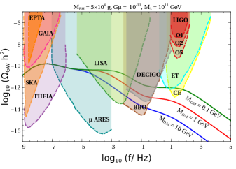
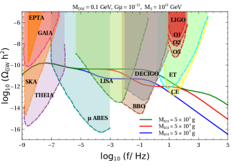
Figure 3: Gravitation wave spectra for the fundamental ($k=1$) mode for different values of DM mass (left panel) and initial PBH mass (right panel), satisfying the condition $\Omega_{\rm DM}h^{2}=0.12$. The experimental sensitivities of SKA Weltman:2018zrl , GAIA Garcia-Bellido:2021zgu , EPTA Kramer_2013 , THEIA Garcia-Bellido:2021zgu , $\mu$ARES Sesana:2019vho , LISA 2017arXiv170200786A , DECIGO Kawamura:2006up , BBO Yagi:2011wg , ET Punturo_2010 , CE LIGOScientific:2016wof and aLIGO LIGOScientific:2014pky are shown as shaded regions of different colours.

Next, we look into the effects of the matter-dominated era arising from PBH (MD1). Here, the expression for the turning point frequency $f_{\Delta}$ given by Eq. (14) is changed because of the other intermediate epochs before BBN. This can be understood as follows. A loop formed at the time $t_{3}$ would contribute to the spectrum much later when it reaches its half-life which is given by Gouttenoire:2019kij

$$\tilde{t}_{M}\simeq\frac{\alpha t_{3}}{2\Gamma G\mu}$$ (18)

The frequency emitted is related to the length of the loop at its half-life time $\left(f(\tilde{t}_{M})=2k/l(\tilde{t}_{M})\right)$ and hence we get

$$\alpha t_{3}\simeq\frac{4}{f}\frac{a(\tilde{t}_{M})}{a(t_{0})}$$ (19)

where $f$ is the frequency observed today. Now, usually $\tilde{t}_{M}$ is in the radiation-dominated era after BBN, which gives us Eq. (14). However, in our case $\tilde{t}_{M}$ would be in the radiation or early matter-dominated era before BBN, which gives us

$$\alpha t_{3}\simeq\frac{4}{f}\frac{a(\tilde{t}_{M})}{a(t_{5})}\frac{a(t_{5})}{a(t_{6})}\frac{a(t_{6})}{a(t_{0})}\simeq\frac{4}{f}\left(\frac{\tilde{t}_{M}}{t_{5}}\right)^{2/3}\left(\frac{t_{5}}{t_{6}}\right)^{1/2}\left(\frac{t_{6}}{t_{0}}\right)^{2/3}$$ (20)

Substituting $\tilde{t}_{M}$ from Eq. (18), we find the turning point frequency, which we call $f^{\prime}_{\Delta}$ to be given by

$$f^{\prime}_{\Delta}\simeq\frac{4}{\alpha^{1/3}t_{3}^{1/3}t_{5}^{2/3}\left(2\Gamma G\mu\right)^{2/3}}\frac{T_{6}}{T_{5}}\left(\frac{g_{*s}(T_{6})}{g_{*s}(T_{5})}\right)^{1/3}z_{\rm eq}^{-1}$$ (21)

Using $t_{3,5}\sim\frac{1}{2T_{3,5}^{2}}$, we get

$$f^{\prime}_{\Delta}\propto T_{3}^{2/3}T_{5}^{1/3}.$$ (22)

Thus, the TPF $f^{\prime}_{\Delta}$ depends not only on the PBH evaporation temperature $T_{3}$, but also on $T_{5}$, i.e, the temperature when $N_{3}$ dominated era ends. Using Eq. (17) and 30, we find $f_{\Delta}\propto\frac{1}{M_{\rm DM}^{1/3}}\frac{1}{m_{\rm in}^{5/3}}$.

Similar turning point frequencies can also be obtained for loops below a critical length $l_{c}=\frac{\mu^{-1/2}}{\left(\Gamma G\mu\right)^{2}}$ Auclair:2019jip , for which particle production becomes dominant over the GW emission. This translates into the bound $G\mu>2.4\times 10^{-16}T_{\Delta}^{4/5}$. In our scenario, we choose $G\mu=10^{-11}$ which is high enough such that the GW emission always dominate. This gives an upper bound on the TPF as $T_{\Delta}\lesssim 5\times 10^{5}$ GeV, and considering $T_{\Delta}=T_{3}=T_{\rm ev}$, we get a lower bound on the initial PBH mass as $m_{\rm in}\gtrsim 2\times 10^{3}$ g.

    

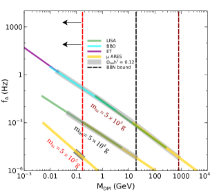
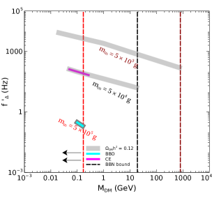
Figure 4: Contours satisfying $\Omega_{\rm DM}h^{2}=0.12$ in the $M_{\rm DM}-f_{\Delta}$ plane (left panel) and the $M_{\rm DM}-f^{\prime}_{\Delta}$ (right panel), along with the sensitivities of future experiments like LISA 2017arXiv170200786A , BBO Yagi:2011wg , ET Punturo_2010 , CE LIGOScientific:2016wof , $\mu$ARES Sesana:2019vho . Here, $G\mu=10^{-11}$ and $M_{3}=10^{11}$ GeV.

We now compute the GW spectra by integrating Eq. (12) over the different cosmological epochs. The temperatures corresponding to the different cosmological backgrounds (see Fig. 1) which would be required in this integration is found by numerically solving the Boltzmann equations (see Appendix B) for $\rho_{\rm BH}$, $\rho_{\rm R}$, $\rho_{\rm DM}$ and $\rho_{\rm N_{3}}$. In Fig. 3, we show the GW spectra for three DM masses (left panel) and three PBH masses (right panel), differing by orders of magnitude. The decay rate of $N_{3}$ is chosen such that $\Omega_{\rm DM}h^{2}=0.12$. As anticipated above, the spectral breaks due to the two early matter-dominated eras can be clearly seen. The first break ($f_{\Delta}$) at the lower frequency, from flat to power-law, depends on the temperature $T_{5}$ which marks the end of $N_{3}$ domination. It is evident here that $f_{\Delta}$ decreases with DM mass $M_{\rm DM}$ and initial PBH mass $m_{\rm in}$. The break from flat to power-law at higher frequencies ($f^{\prime}_{\Delta}$) is related to PBH evaporation at the temperature $T_{3}$, and a higher evaporation temperature (lower $m_{\rm in}$) implies break at a higher frequency (right panel). However, as discussed above, this break also depends on the other intermediate eras before BBN, specifically on the temperature $T_{5}$ (see Eq. (22)). This is apparent from the left panel where even for the same initial PBH mass $m_{\rm in}$ (and hence same $T_{3}$), the break occurs at different frequencies. Note that there appears another break in the spectrum at the middle, from power-law to flat, which can also be probed in the detectors. Finally, recall that we are using only the $k=1$ mode for computing the GW spectra, and taking the effects of the higher modes will lead to a different power-law dependence after the TPF $f_{\Delta}$ with a smaller slope ($f^{-1/3}$). This might cause a rise in the amplitude after $f_{\Delta}$. However, the TPF $f^{\prime}_{\Delta}$ is expected to remain almost unchanged.

In the left panel of Fig. 4, we show the contours in the $M_{\rm DM}-f_{\Delta}$ plane (grey-shaded) which satisfies the correct DM relic, along with the sensitivities of the GW experiments which can probe them. We find our numerical results to agree with our analytical estimates derived earlier upto a difference of around $\mathcal{O}(1)$. As expected, the contours move up when we increase the PBH mass $m_{\rm in}$. The upper bound on the DM mass appears since $N_{3}$ has to decay before BBN. Note that this bound changes with $m_{\rm in}$, since a heavier PBH evaporates at a lower temperature, closer to BBN. Decreasing DM mass leads to $\Omega_{\rm DM}h^{2}<0.12$, which gives us a lower bound on DM mass. In the right panel of figure 4, for the same PBH masses we show the corresponding predictions at the higher frequencies, i.e. the $M_{\rm DM}-f^{\prime}_{\Delta}$ plane. As we can see, for lighter PBH and heavier DM, $f^{\prime}_{\Delta}$ falls outside the sensitivities. Finally, in Table 1 , we provide some benchmark values of DM mass $M_{\rm DM}$ and PBH mass $m_{\rm in}$ along with the GW experiments which can probe the corresponding spectral breaks.

BP	$m_{\text{in}}$(g)	$M_{\text{DM}}$(GeV)	$1^{\text{st}}~{}\text{TPF}$	$2^{\text{nd}}~{}\text{TPF}$	$3^{\text{rd}}~{}\text{TPF}$
BP1	$3\times 10^{3}$	0.01	ET	NONE	NONE
BP2	$1.2\times 10^{4}$	5	LISA, DECIGO, BBO	CE	NONE
BP3	$5\times 10^{4}$	0.1	LISA	DECIGO, BBO	CE
BP4	$10^{5}$	0.3	LISA, $\mu$ARES	DECIGO, BBO	NONE
BP5	$5\times 10^{5}$	0.15	$\mu$ARES	LISA	DECIGO, BBO

Table 1: Some benchmark points (BP) of $M_{\rm DM}$ and $m_{\rm in}$ along with the GW experiments which can probe the $1^{\rm st}$ TPF($f_{\Delta}$) from flat to power-law, $2^{\rm nd}$ TPF from power-law to flat and $3^{\rm rd}$ TPF($f^{\prime}_{\Delta}$) from flat to power-law.

V Conclusion

We have studied the possibility of probing a high scale seesaw origin of neutrino mass and PBH generated dark matter scenario simultaneously by future observation of stochastic gravitational wave background with multiple tilts or spectral breaks. A high scale $U(1)$ gauge symmetry breaking not only generates the seesaw scale dynamically but also leads to the formation of cosmic strings responsible for generating stochastic GW later. Considering purely gravitational dark matter originating from an intermediate primordial black hole dominated epoch, we also incorporate the presence of an additional diluter to bring DM overproduction from PBH under control. The required relic abundance of DM around the MeV-TeV ballpark, which we consider in this work, forces the diluter to be sufficiently long-lived leading to a second early matter-domination epoch in addition to the PBH dominated one. While cosmic strings typically leads to a scale invariant GW spectrum, the presence of two different early matter domination in our setup leads to multiple spectral breaks. After solving the relevant Boltzmann equations numerically for DM relic, we make an estimate of the spectral break frequencies both analytically as well as numerically and find interesting correlations with DM mass. As summarised in Fig. 4 and Table 1, the spectral break frequencies can be probed at multiple future experiments depending upon the DM mass. Clearly, the parameter space corresponding to a wide range of DM masses remain within experimental reach, although the three spectral breaks simultaneously remain within the experimental sensitivities only when the DM mass is restricted to be in the sub-GeV ballpark. While high scale seesaw and gravitational DM have no scope of direct experimental probe, our setup provides an interesting near future probe of such scenarios via multiple spectral breaks in gravitational wave spectrum generated by cosmic strings.

Appendix A PBH fact-sheet

The mass of the black hole from gravitational collapse is typically close to the value enclosed by the post-inflation particle horizon and is given by Fujita:2014hha ; Masina:2020xhk

$$m_{\text{BH}}^{\rm in}=\frac{4}{3}\,\pi\,\gamma\,\Bigl{(}\frac{1}{\mathcal{H}\left(T_{\text{in}}\right)}\Bigr{)}^{3}\,\rho_{\text{rad}}\left(T_{\text{in}}\right)\,$$ (23)

with

$$\rho_{\text{rad}}\left(T_{\text{in}}\right)=\frac{3}{8\,\pi}\,\mathcal{H}\left(T_{\text{in}}\right)^{2}\,M_{\text{pl}}^{2}\,$$ (24)

where $\mathcal{H}$ is the Hubble parameter. As mentioned earlier, PBHs are produced during the radiation dominated epoch, when the SM plasma has a temperature $T=T_{\text{in}}$ which is given by

$$T_{\text{in}}=\Biggl{(}\frac{45\,\gamma^{2}}{16\,\pi^{3}\,g_{\star}\left(T_{\text{in}}\right)}\Biggr{)}^{1/4}\,\sqrt{\frac{M_{\text{pl}}}{m_{\text{BH}}(T_{\text{in}})}}\,M_{\text{pl}}\,.$$ (25)

Once formed, a PBH evaporates efficiently into particles lighter than its instantaneous temperature $T_{\text{BH}}$ defined as Hawking:1975vcx

$$T_{\rm BH}=\frac{1}{8\pi\,G\,m_{\rm BH}}\approx 1.06~{}\left(\frac{10^{13}\;{\rm g}}{m_{\rm BH}}\right)~{}{\rm GeV}\,,$$ (26)

with $G$ being the universal gravitational constant. The mass loss rate in this scenario is parametrised as MacGibbon:1991tj

$$\frac{dm_{\text{BH}}(t)}{dt}=-\frac{\mathcal{G}\,g_{\star}\left(T_{\text{BH}}\right)}{30720\,\pi}\,\frac{M_{\text{pl}}^{4}}{m_{\text{BH}}^{\rm in}(t)^{2}}\,.$$ (27)

Under the assumption that $g_{\star}$ does not change during the PBH evolution, integrating Eq. (27), we end up with the PBH mass evolution equation as

$$m_{\text{BH}}(t)=m_{\text{BH}}(T_{\text{in}})\Bigl{(}1-\frac{t-t_{\text{in}}}{\tau}\Bigr{)}^{1/3}\,,$$ (28)

with

$$\tau=\frac{10240\,\pi\,m_{\text{BH}}^{\rm in3}}{\mathcal{G}\,g_{\star}(T_{\text{BH}})\,M_{\text{pl}}^{4}}\,,$$ (29)

as the PBH lifetime. Here onward we will use $m_{\text{in}}(T_{\text{in}})$ simply as $m_{\text{in}}$. One can calculate the evaporation temperature by considering $H(T_{\text{evap}})\sim\frac{1}{\tau^{2}}\sim\rho_{\text{rad}}(T_{\text{evap}})$,

$$T_{\text{ev}}\equiv\Bigl{(}\frac{45\,M_{\text{pl}}^{2}}{16\,\pi^{3}\,g_{\star}\left(T_{\text{evap}}\right)\,\tau^{2}}\Bigr{)}^{1/4}\,.$$ (30)

However, if the PBH component dominates at some point the total energy density of the universe, the SM temperature just after the complete evaporation of PBHs is: $\overline{T}_{\text{evap}}=2/\sqrt{3}\,T_{\text{evap}}$ Bernal:2020bjf .

Appendix B Coupled Boltzmann Equations

The relevant coupled Boltzmann equations (BEQ) in the present framework reads Perez-Gonzalez:2020vnz ; JyotiDas:2021shi ; Barman:2021ost

$$\frac{dm_{\text{BH}}}{da}=-\frac{\kappa}{a\,\mathcal{H}}\,\epsilon(m_{\text{BH}})\,\left(\frac{1\text{g}}{m_{\rm BH}}\right)^{2}\,,$$

$$\frac{d\widetilde{\rho}_{R}}{da}=-\frac{\epsilon_{\text{SM}}(m_{\text{BH}})}{\epsilon(m_{\text{BH}})}\,\frac{a}{m_{\text{BH}}}\,\frac{dm_{\text{BH}}}{da}\,\widetilde{\rho}_{\text{BH}}+\frac{a}{\mathcal{H}}\Gamma_{3}M_{3}\widetilde{n}_{N_{3}}^{\text{BH}}\,,$$

$$\frac{d\widetilde{\rho}_{\text{BH}}}{da}=\frac{1}{m_{\text{BH}}}\,\frac{dm_{\text{BH}}}{da}\,\widetilde{\rho}_{\text{BH}}\,,$$

$$a\mathcal{H}\frac{d\widetilde{n}_{N_{3}}^{\text{BH}}}{da}=\Gamma_{\text{BH}\to N_{3}}\,\frac{\widetilde{\rho}_{BH}}{m_{BH}}-\Gamma_{3}\widetilde{n}_{N_{3}}^{\text{BH}}$$

$$a\mathcal{H}\frac{d\widetilde{n}_{DM}^{\text{BH}}}{da}=\Gamma_{\text{BH}\to DM}\,\frac{\widetilde{\rho}_{BH}}{m_{BH}}$$

$$\frac{dT}{da}=-\frac{T}{\Delta}\Biggl{[}\frac{1}{a}+\frac{\epsilon_{\text{SM}}(m_{\text{BH}})}{\epsilon(m_{\text{BH}})}\,\frac{1}{m_{\text{BH}}}\,\frac{dm_{\text{BH}}}{da}\,\frac{g_{\star}(T)}{g_{\star s}(T)}\,a\,\frac{\widetilde{\rho}_{BH}}{4\,\widetilde{\rho}_{R}}+\frac{\Gamma_{3}M_{3}}{3\mathcal{H}~{}s~{}a^{4}}\widetilde{n}_{N_{3}}^{\text{BH}}\Biggr{]}\,.$$ (31)

Here, $\widetilde{\rho}_{R}$ and $\widetilde{\rho}_{\text{BH}}$ denotes the comoving energy density of radiation and PBH, $\mathcal{H}$ is the Hubble parameter, whereas $\widetilde{n}_{N3}$ and $\widetilde{n}_{DM}$ represent the comoving number densities of $N_{3}$ and DM respectively.

References

- (1) Particle Data Group Collaboration, P. A. Zyla et al., Review of Particle Physics, PTEP 2020 (2020), no. 8 083C01.
- (2) R. N. Mohapatra et al., Theory of neutrinos: A White paper, Rept. Prog. Phys. 70 (2007) 1757–1867, [hep-ph/0510213].
- (3) P. Minkowski, at a Rate of One Out of Muon Decays?, Phys. Lett. B 67 (1977) 421–428.
- (4) M. Gell-Mann, P. Ramond, and R. Slansky, Complex Spinors and Unified Theories, Conf. Proc. C 790927 (1979) 315–321, [arXiv:1306.4669].
- (5) R. N. Mohapatra and G. Senjanovic, Neutrino Mass and Spontaneous Parity Nonconservation, Phys. Rev. Lett. 44 (1980) 912.
- (6) J. Schechter and J. Valle, Neutrino Masses in SU(2) x U(1) Theories, Phys. Rev. D 22 (1980) 2227.
- (7) R. N. Mohapatra and G. Senjanovic, Neutrino Masses and Mixings in Gauge Models with Spontaneous Parity Violation, Phys. Rev. D 23 (1981) 165.
- (8) G. Lazarides, Q. Shafi, and C. Wetterich, Proton Lifetime and Fermion Masses in an SO(10) Model, Nucl. Phys. B 181 (1981) 287–300.
- (9) C. Wetterich, Neutrino Masses and the Scale of B-L Violation, Nucl. Phys. B187 (1981) 343–375.
- (10) J. Schechter and J. W. F. Valle, Neutrino Decay and Spontaneous Violation of Lepton Number, Phys. Rev. D25 (1982) 774.
- (11) R. Foot, H. Lew, X. He, and G. C. Joshi, Seesaw Neutrino Masses Induced by a Triplet of Leptons, Z. Phys. C 44 (1989) 441.
- (12) J. A. Dror, T. Hiramatsu, K. Kohri, H. Murayama, and G. White, Testing the Seesaw Mechanism and Leptogenesis with Gravitational Waves, Phys. Rev. Lett. 124 (2020), no. 4 041804, [arXiv:1908.03227].
- (13) S. Blasi, V. Brdar, and K. Schmitz, Fingerprint of low-scale leptogenesis in the primordial gravitational-wave spectrum, Phys. Rev. Res. 2 (2020), no. 4 043321, [arXiv:2004.02889].
- (14) B. Fornal and B. Shams Es Haghi, Baryon and Lepton Number Violation from Gravitational Waves, Phys. Rev. D 102 (2020), no. 11 115037, [arXiv:2008.05111].
- (15) R. Samanta and S. Datta, Gravitational wave complementarity and impact of NANOGrav data on gravitational leptogenesis, JHEP 05 (2021) 211, [arXiv:2009.13452].
- (16) B. Barman, D. Borah, A. Dasgupta, and A. Ghoshal, Probing High Scale Dirac Leptogenesis via Gravitational Waves from Domain Walls, arXiv:2205.03422.
- (17) P. Huang and K.-P. Xie, Leptogenesis triggered by a first-order phase transition, arXiv:2206.04691.
- (18) A. Dasgupta, P. S. B. Dev, A. Ghoshal, and A. Mazumdar, Gravitational Wave Pathway to Testable Leptogenesis, arXiv:2206.07032.
- (19) N. Okada and O. Seto, Probing the seesaw scale with gravitational waves, Phys. Rev. D 98 (2018), no. 6 063532, [arXiv:1807.00336].
- (20) T. Hasegawa, N. Okada, and O. Seto, Gravitational waves from the minimal gauged model, Phys. Rev. D 99 (2019), no. 9 095039, [arXiv:1904.03020].
- (21) D. Borah, A. Dasgupta, and I. Saha, Leptogenesis and Dark Matter Through Relativistic Bubble Walls with Observable Gravitational Waves, arXiv:2207.14226.
- (22) Planck Collaboration, N. Aghanim et al., Planck 2018 results. VI. Cosmological parameters, arXiv:1807.06209.
- (23) E. W. Kolb and M. S. Turner, The Early Universe, vol. 69. 1990.
- (24) LUX-ZEPLIN Collaboration, J. Aalbers et al., First Dark Matter Search Results from the LUX-ZEPLIN (LZ) Experiment, arXiv:2207.03764.
- (25) C. Yuan, R. Brito, and V. Cardoso, Probing ultralight dark matter with future ground-based gravitational-wave detectors, Phys. Rev. D 104 (2021), no. 4 044011, [arXiv:2106.00021].
- (26) L. Tsukada, R. Brito, W. E. East, and N. Siemonsen, Modeling and searching for a stochastic gravitational-wave background from ultralight vector bosons, Phys. Rev. D 103 (2021), no. 8 083005, [arXiv:2011.06995].
- (27) A. Chatrchyan and J. Jaeckel, Gravitational waves from the fragmentation of axion-like particle dark matter, JCAP 02 (2021) 003, [arXiv:2004.07844].
- (28) L. Bian, X. Liu, and K.-P. Xie, Probing superheavy dark matter with gravitational waves, JHEP 11 (2021) 175, [arXiv:2107.13112].
- (29) R. Samanta and F. R. Urban, Testing Super Heavy Dark Matter from Primordial Black Holes with Gravitational Waves, arXiv:2112.04836.
- (30) D. Borah, S. Jyoti Das, A. K. Saha, and R. Samanta, Probing WIMP dark matter via gravitational waves’ spectral shapes, Phys. Rev. D 106 (2022), no. 1 L011701, [arXiv:2202.10474].
- (31) A. Azatov, M. Vanvlasselaer, and W. Yin, Dark Matter production from relativistic bubble walls, JHEP 03 (2021) 288, [arXiv:2101.05721].
- (32) A. Azatov, G. Barni, S. Chakraborty, M. Vanvlasselaer, and W. Yin, Ultra-relativistic bubbles from the simplest Higgs portal and their cosmological consequences, arXiv:2207.02230.
- (33) I. Baldes, Y. Gouttenoire, and F. Sala, Hot and Heavy Dark Matter from Supercooling, arXiv:2207.05096.
- (34) B. Barman, D. Borah, S. Das Jyoti, and R. Roshan, Cogenesis of Baryon Asymmetry and Gravitational Dark Matter from PBH, arXiv:2204.10339.
- (35) T. W. B. Kibble, Topology of Cosmic Domains and Strings, J. Phys. A 9 (1976) 1387–1398.
- (36) H. B. Nielsen and P. Olesen, Vortex Line Models for Dual Strings, Nucl. Phys. B 61 (1973) 45–61.
- (37) A. Vilenkin, Gravitational radiation from cosmic strings, Phys. Lett. B 107 (1981) 47–50.
- (38) N. Turok, Grand Unified Strings and Galaxy Formation, Nucl. Phys. B 242 (1984) 520–541.
- (39) Y. Cui, M. Lewicki, D. E. Morrissey, and J. D. Wells, Cosmic Archaeology with Gravitational Waves from Cosmic Strings, Phys. Rev. D 97 (2018), no. 12 123505, [arXiv:1711.03104].
- (40) Y. Cui, M. Lewicki, D. E. Morrissey, and J. D. Wells, Probing the pre-BBN universe with gravitational waves from cosmic strings, JHEP 01 (2019) 081, [arXiv:1808.08968].
- (41) Y. Gouttenoire, G. Servant, and P. Simakachorn, Beyond the Standard Models with Cosmic Strings, JCAP 07 (2020) 032, [arXiv:1912.02569].
- (42) X. He, G. C. Joshi, H. Lew, and R. Volkas, NEW Z-prime PHENOMENOLOGY, Phys. Rev. D 43 (1991) 22–24.
- (43) X.-G. He, G. C. Joshi, H. Lew, and R. R. Volkas, Simplest Z-prime model, Phys. Rev. D 44 (1991) 2118–2132.
- (44) K. Asai, K. Hamaguchi, and N. Nagata, Predictions for the neutrino parameters in the minimal gauged U(1) model, Eur. Phys. J. C 77 (2017), no. 11 763, [arXiv:1705.00419].
- (45) D. Borah, A. Dasgupta, and D. Mahanta, TeV scale resonant leptogenesis with L-L gauge symmetry in light of the muon g-2, Phys. Rev. D 104 (2021), no. 7 075006, [arXiv:2106.14410].
- (46) T. Fujita, M. Kawasaki, K. Harigaya, and R. Matsuda, Baryon asymmetry, dark matter, and density perturbation from primordial black holes, Phys. Rev. D 89 (2014), no. 10 103501, [arXiv:1401.1909].
- (47) I. Masina, Dark matter and dark radiation from evaporating primordial black holes, Eur. Phys. J. Plus 135 (2020), no. 7 552, [arXiv:2004.04740].
- (48) B. Carr, K. Kohri, Y. Sendouda, and J. Yokoyama, Constraints on Primordial Black Holes, arXiv:2002.12778.
- (49) S. W. Hawking, Black hole explosions, Nature 248 (1974) 30–31.
- (50) S. W. Hawking, Particle Creation by Black Holes, Commun. Math. Phys. 43 (1975) 199–220. [Erratum: Commun.Math.Phys. 46, 206 (1976)].
- (51) L. Morrison, S. Profumo, and Y. Yu, Melanopogenesis: Dark Matter of (almost) any Mass and Baryonic Matter from the Evaporation of Primordial Black Holes weighing a Ton (or less), JCAP 05 (2019) 005, [arXiv:1812.10606].
- (52) P. Gondolo, P. Sandick, and B. Shams Es Haghi, Effects of primordial black holes on dark matter models, Phys. Rev. D 102 (2020), no. 9 095018, [arXiv:2009.02424].
- (53) N. Bernal and O. Zapata, Dark Matter in the Time of Primordial Black Holes, JCAP 03 (2021) 015, [arXiv:2011.12306].
- (54) A. M. Green, Supersymmetry and primordial black hole abundance constraints, Phys. Rev. D 60 (1999) 063516, [astro-ph/9903484].
- (55) M. Y. Khlopov, A. Barrau, and J. Grain, Gravitino production by primordial black hole evaporation and constraints on the inhomogeneity of the early universe, Class. Quant. Grav. 23 (2006) 1875–1882, [astro-ph/0406621].
- (56) D.-C. Dai, K. Freese, and D. Stojkovic, Constraints on dark matter particles charged under a hidden gauge group from primordial black holes, JCAP 06 (2009) 023, [arXiv:0904.3331].
- (57) R. Allahverdi, J. Dent, and J. Osinski, Nonthermal production of dark matter from primordial black holes, Phys. Rev. D 97 (2018), no. 5 055013, [arXiv:1711.10511].
- (58) O. Lennon, J. March-Russell, R. Petrossian-Byrne, and H. Tillim, Black Hole Genesis of Dark Matter, JCAP 04 (2018) 009, [arXiv:1712.07664].
- (59) D. Hooper, G. Krnjaic, and S. D. McDermott, Dark Radiation and Superheavy Dark Matter from Black Hole Domination, JHEP 08 (2019) 001, [arXiv:1905.01301].
- (60) A. Chaudhuri and A. Dolgov, PBH evaporation, baryon asymmetry,and dark matter, arXiv:2001.11219.
- (61) I. Baldes, Q. Decant, D. C. Hooper, and L. Lopez-Honorez, Non-Cold Dark Matter from Primordial Black Hole Evaporation, JCAP 08 (2020) 045, [arXiv:2004.14773].
- (62) N. Bernal and O. Zapata, Gravitational dark matter production: primordial black holes and UV freeze-in, Phys. Lett. B 815 (2021) 136129, [arXiv:2011.02510].
- (63) N. Bernal and O. Zapata, Self-interacting Dark Matter from Primordial Black Holes, JCAP 03 (2021) 007, [arXiv:2010.09725].
- (64) B. C. Lacki and J. F. Beacom, Primordial Black Holes as Dark Matter: Almost All or Almost Nothing, Astrophys. J. Lett. 720 (2010) L67–L71, [arXiv:1003.3466].
- (65) S. M. Boucenna, F. Kuhnel, T. Ohlsson, and L. Visinelli, Novel Constraints on Mixed Dark-Matter Scenarios of Primordial Black Holes and WIMPs, JCAP 07 (2018) 003, [arXiv:1712.06383].
- (66) J. Adamek, C. T. Byrnes, M. Gosenca, and S. Hotchkiss, WIMPs and stellar-mass primordial black holes are incompatible, Phys. Rev. D 100 (2019), no. 2 023506, [arXiv:1901.08528].
- (67) B. Carr, F. Kuhnel, and L. Visinelli, Black holes and WIMPs: all or nothing or something else, Mon. Not. Roy. Astron. Soc. 506 (2021), no. 3 3648–3661, [arXiv:2011.01930].
- (68) I. Masina, Dark matter and dark radiation from evaporating Kerr primordial black holes, arXiv:2103.13825.
- (69) N. Bernal, Y. F. Perez-Gonzalez, Y. Xu, and O. Zapata, ALP Dark Matter in a Primordial Black Hole Dominated Universe, arXiv:2110.04312.
- (70) N. Bernal, F. Hajkarim, and Y. Xu, Axion Dark Matter in the Time of Primordial Black Holes, Phys. Rev. D 104 (2021) 075007, [arXiv:2107.13575].
- (71) P. Sandick, B. S. Es Haghi, and K. Sinha, Asymmetric reheating by primordial black holes, Phys. Rev. D 104 (2021), no. 8 083523, [arXiv:2108.08329].
- (72) A. Cheek, L. Heurtier, Y. F. Perez-Gonzalez, and J. Turner, Primordial Black Hole Evaporation and Dark Matter Production: II. Interplay with the Freeze-In/Out Mechanism, arXiv:2107.00016.
- (73) A. Cheek, L. Heurtier, Y. F. Perez-Gonzalez, and J. Turner, Primordial Black Hole Evaporation and Dark Matter Production: I. Solely Hawking radiation, arXiv:2107.00013.
- (74) B. J. Carr, Some cosmological consequences of primordial black-hole evaporations, Astrophys. J. 206 (1976) 8–25.
- (75) D. Baumann, P. J. Steinhardt, and N. Turok, Primordial Black Hole Baryogenesis, hep-th/0703250.
- (76) A. Hook, Baryogenesis from Hawking Radiation, Phys. Rev. D 90 (2014), no. 8 083535, [arXiv:1404.0113].
- (77) Y. Hamada and S. Iso, Baryon asymmetry from primordial black holes, PTEP 2017 (2017), no. 3 033B02, [arXiv:1610.02586].
- (78) D. Hooper and G. Krnjaic, GUT Baryogenesis With Primordial Black Holes, Phys. Rev. D 103 (2021), no. 4 043504, [arXiv:2010.01134].
- (79) Y. F. Perez-Gonzalez and J. Turner, Assessing the tension between a black hole dominated early universe and leptogenesis, arXiv:2010.03565.
- (80) S. Datta, A. Ghosal, and R. Samanta, Baryogenesis from ultralight primordial black holes and strong gravitational waves from cosmic strings, JCAP 08 (2021) 021, [arXiv:2012.14981].
- (81) S. Jyoti Das, D. Mahanta, and D. Borah, Low scale leptogenesis and dark matter in the presence of primordial black holes, arXiv:2104.14496.
- (82) N. Smyth, L. Santos-Olmsted, and S. Profumo, Gravitational Baryogenesis and Dark Matter from Light Black Holes, arXiv:2110.14660.
- (83) B. Barman, D. Borah, S. J. Das, and R. Roshan, Non-thermal origin of asymmetric dark matter from inflaton and primordial black holes, JCAP 03 (2022), no. 03 031, [arXiv:2111.08034].
- (84) N. Bernal, C. S. Fong, Y. F. Perez-Gonzalez, and J. Turner, Rescuing High-Scale Leptogenesis using Primordial Black Holes, arXiv:2203.08823.
- (85) A. Ambrosone, R. Calabrese, D. F. G. Fiorillo, G. Miele, and S. Morisi, Towards baryogenesis via absorption from primordial black holes, Phys. Rev. D 105 (2022), no. 4 045001, [arXiv:2106.11980].
- (86) N. Bhaumik, A. Ghoshal, and M. Lewicki, Doubly peaked induced stochastic gravitational wave background: testing baryogenesis from primordial black holes, JHEP 07 (2022) 130, [arXiv:2205.06260].
- (87) R. Diamanti, S. Ando, S. Gariazzo, O. Mena, and C. Weniger, Cold dark matter plus not-so-clumpy dark relics, JCAP 06 (2017) 008, [arXiv:1701.03128].
- (88) M. Garny, M. Sandora, and M. S. Sloth, Planckian Interacting Massive Particles as Dark Matter, Phys. Rev. Lett. 116 (2016), no. 10 101302, [arXiv:1511.03278].
- (89) Y. Tang and Y.-L. Wu, On Thermal Gravitational Contribution to Particle Production and Dark Matter, Phys. Lett. B 774 (2017) 676–681, [arXiv:1708.05138].
- (90) M. Garny, A. Palessandro, M. Sandora, and M. S. Sloth, Theory and Phenomenology of Planckian Interacting Massive Particles as Dark Matter, JCAP 02 (2018) 027, [arXiv:1709.09688].
- (91) N. Bernal, M. Dutra, Y. Mambrini, K. Olive, M. Peloso, and M. Pierre, Spin-2 Portal Dark Matter, Phys. Rev. D 97 (2018), no. 11 115020, [arXiv:1803.01866].
- (92) B. Barman and N. Bernal, Gravitational SIMPs, JCAP 06 (2021) 011, [arXiv:2104.10699].
- (93) C. Ringeval, M. Sakellariadou, and F. Bouchet, Cosmological evolution of cosmic string loops, JCAP 02 (2007) 023, [astro-ph/0511646].
- (94) J. J. Blanco-Pillado, K. D. Olum, and B. Shlaer, Large parallel cosmic string simulations: New results on loop production, Phys. Rev. D 83 (2011) 083514, [arXiv:1101.5173].
- (95) NANOGrav Collaboration, Z. Arzoumanian et al., The NANOGrav 12.5 yr Data Set: Search for an Isotropic Stochastic Gravitational-wave Background, Astrophys. J. Lett. 905 (2020), no. 2 L34, [arXiv:2009.04496].
- (96) B. Goncharov et al., On the Evidence for a Common-spectrum Process in the Search for the Nanohertz Gravitational-wave Background with the Parkes Pulsar Timing Array, Astrophys. J. Lett. 917 (2021), no. 2 L19, [arXiv:2107.12112].
- (97) J. Ellis and M. Lewicki, Cosmic String Interpretation of NANOGrav Pulsar Timing Data, Phys. Rev. Lett. 126 (2021), no. 4 041304, [arXiv:2009.06555].
- (98) S. Blasi, V. Brdar, and K. Schmitz, Has NANOGrav found first evidence for cosmic strings?, Phys. Rev. Lett. 126 (2021), no. 4 041305, [arXiv:2009.06607].
- (99) W. Buchmüller, V. Domcke, K. Kamada, and K. Schmitz, The Gravitational Wave Spectrum from Cosmological Breaking, JCAP 10 (2013) 003, [arXiv:1305.3392].
- (100) W. Buchmuller, V. Domcke, H. Murayama, and K. Schmitz, Probing the scale of grand unification with gravitational waves, Phys. Lett. B 809 (2020) 135764, [arXiv:1912.03695].
- (101) S. F. King, S. Pascoli, J. Turner, and Y.-L. Zhou, Gravitational Waves and Proton Decay: Complementary Windows into Grand Unified Theories, Phys. Rev. Lett. 126 (2021), no. 2 021802, [arXiv:2005.13549].
- (102) W. Buchmuller, V. Domcke, and K. Schmitz, Stochastic gravitational-wave background from metastable cosmic strings, JCAP 12 (2021), no. 12 006, [arXiv:2107.04578].
- (103) M. A. Masoud, M. U. Rehman, and Q. Shafi, Sneutrino tribrid inflation, metastable cosmic strings and gravitational waves, JCAP 11 (2021) 022, [arXiv:2107.09689].
- (104) A. Afzal, W. Ahmed, M. U. Rehman, and Q. Shafi, -hybrid Inflation, Gravitino Dark Matter and Stochastic Gravitational Wave Background from Cosmic Strings, arXiv:2202.07386.
- (105) A. Vilenkin, Cosmic string dynamics with friction, Phys. Rev. D 43 (1991) 1060–1062.
- (106) D. P. Bennett and F. R. Bouchet, Evidence for a Scaling Solution in Cosmic String Evolution, Phys. Rev. Lett. 60 (1988) 257.
- (107) D. P. Bennett and F. R. Bouchet, Cosmic string evolution, Phys. Rev. Lett. 63 (1989) 2776.
- (108) T. Vachaspati and A. Vilenkin, Gravitational Radiation from Cosmic Strings, Phys. Rev. D 31 (1985) 3052.
- (109) J. J. Blanco-Pillado, K. D. Olum, and B. Shlaer, The number of cosmic string loops, Phys. Rev. D 89 (2014), no. 2 023512, [arXiv:1309.6637].
- (110) C. J. A. P. Martins and E. P. S. Shellard, Quantitative string evolution, Phys. Rev. D 54 (1996) 2535–2556, [hep-ph/9602271].
- (111) C. J. A. P. Martins and E. P. S. Shellard, Extending the velocity dependent one scale string evolution model, Phys. Rev. D 65 (2002) 043514, [hep-ph/0003298].
- (112) P. Auclair et al., Probing the gravitational wave background from cosmic strings with LISA, JCAP 04 (2020) 034, [arXiv:1909.00819].
- (113) J. J. Blanco-Pillado and K. D. Olum, Stochastic gravitational wave background from smoothed cosmic string loops, Phys. Rev. D 96 (2017), no. 10 104046, [arXiv:1709.02693].
- (114) T. Charnock, A. Avgoustidis, E. J. Copeland, and A. Moss, CMB constraints on cosmic strings and superstrings, Phys. Rev. D 93 (2016), no. 12 123503, [arXiv:1603.01275].
- (115) Y. Gouttenoire, G. Servant, and P. Simakachorn, BSM with Cosmic Strings: Heavy, up to EeV mass, Unstable Particles, JCAP 07 (2020) 016, [arXiv:1912.03245].
- (116) A. Weltman et al., Fundamental physics with the Square Kilometre Array, Publ. Astron. Soc. Austral. 37 (2020) e002, [arXiv:1810.02680].
- (117) J. Garcia-Bellido, H. Murayama, and G. White, Exploring the Early Universe with Gaia and THEIA, arXiv:2104.04778.
- (118) M. Kramer and D. J. Champion, The european pulsar timing array and the large european array for pulsars, Classical and Quantum Gravity 30 (nov, 2013) 224009.
- (119) A. Sesana et al., Unveiling the gravitational universe at -Hz frequencies, Exper. Astron. 51 (2021), no. 3 1333–1383, [arXiv:1908.11391].
- (120) LISA Collaboration, P. Amaro-Seoane et al, Laser Interferometer Space Antenna, arXiv e-prints (Feb., 2017) arXiv:1702.00786, [arXiv:1702.00786].
- (121) S. Kawamura et al., The Japanese space gravitational wave antenna DECIGO, Class. Quant. Grav. 23 (2006) S125–S132.
- (122) K. Yagi and N. Seto, Detector configuration of DECIGO/BBO and identification of cosmological neutron-star binaries, Phys. Rev. D 83 (2011) 044011, [arXiv:1101.3940]. [Erratum: Phys.Rev.D 95, 109901 (2017)].
- (123) ET Collaboration Collaboration, M. Punturo et al, The einstein telescope: a third-generation gravitational wave observatory, Classical and Quantum Gravity 27 (sep, 2010) 194002.
- (124) LIGO Scientific Collaboration, B. P. Abbott et al., Exploring the Sensitivity of Next Generation Gravitational Wave Detectors, Class. Quant. Grav. 34 (2017), no. 4 044001, [arXiv:1607.08697].
- (125) LIGO Scientific Collaboration, J. Aasi et al., Advanced LIGO, Class. Quant. Grav. 32 (2015) 074001, [arXiv:1411.4547].
- (126) P. Auclair, D. A. Steer, and T. Vachaspati, Particle emission and gravitational radiation from cosmic strings: observational constraints, Phys. Rev. D 101 (2020), no. 8 083511, [arXiv:1911.12066].
- (127) J. H. MacGibbon, Quark and gluon jet emission from primordial black holes. 2. The Lifetime emission, Phys. Rev. D 44 (1991) 376–392.