A physically-informed Deep-Learning approach for locating sources in a waveguide

Abstract

Inverse source problems are central to many applications in acoustics, geophysics, non-destructive testing, and more. Traditional imaging methods suffer from the resolution limit, preventing distinction of sources separated by less than the emitted wavelength. In this work we propose a method based on physically-informed neural-networks for solving the source refocusing problem, constructing a novel loss term which promotes super-resolving capabilities of the network and is based on the physics of wave propagation. We demonstrate the approach in the setup of imaging an a-priori unknown number of point sources in a two-dimensional rectangular waveguide from measurements of wavefield recordings along a vertical cross-section. The results show the ability of the method to approximate the locations of sources with high accuracy, even when placed close to each other.

Keywords First keyword  $\cdot$ Second keyword  $\cdot$ More

1 Introduction

A large class of inverse problems in imaging aims at recovering locations of sources of waves from sensor measurements of the wavefield radiated by these sources. Many applications for locating sources exist in the literature, in various fields such as acoustics, geophysics, non-destructive evaluation and more [1, 2, 3, 4, 5, 6, 7, 8, 9, 10].

These “inverse source” problems are usually ill-posed. The incomplete data provided only by a few sensors makes the solution very sensitive to that data. In addition, traditional imaging methods such as Kirchhoff migration suffer from the so-called resolution limit, when close-by sources cannot be distinguished from each other in the image due to the nonzero width of the Green’s function. Various super-resolution techniques can in principle overcome these limitations, however at the expense of extreme sensitivity to noise in the data and highly nontrivial mathematical theory, which is currently applicable only in a limited number of cases (see Section 2).

The use of machine-learning (ML) for solving inverse problems is spreading fast within the scientific community [11, 12, 13, 14]. According to this paradigm, many PDE-based inverse problems of the form $A(x)\approx y$, including the one in this paper, can be formulated as data-driven problems, i.e. searching for a general neural network model ${\cal NN}_{\theta}$ whose weights $\theta$ are learned by fitting a vector of model parameters $\{x_{i}\}$ to the corresponding measurements $y_{i}\approx A(x_{i})$, requiring that ${\cal NN}_{\theta}(y_{i})\approx x_{i}$ for all $\{(x_{i},y_{i})\}$ in a large training set. The advances in computation capabilities and ease of use of the ML libraries have opened doors for many researchers to investigate ML based inverse solutions corresponding to various forward models $A$. In particular, ML-based inversion techniques can be used with highly nonlinear $A$, are relatively robust to perturbations, and can provide real-time inference (in contrast with traditional optimization-based methods where the solution to a single problem instance $A(x^{*})\approx y^{*}$ may require substantial computational resources).

ML-based methods also have their drawbacks. In a classical ML approach to inverse problems, the structure of the mapping ${\cal NN}_{\theta}$ is very general and independent of the governing PDE. Therefore, ML methods may severely underperform when tested on a slightly different task than the one they were trained for. For example, using a model that was trained to find point sources will struggle when injecting data produced by using an extended source.

Deep-learning (DL) refers to a subset of ML methods, where the function ${\cal NN}_{\theta}$ is composed of a very large number of layers (which makes the network “deep”), where each layer connects to the next by a pointwise, usually nonlinear, transformation. While the study of DL is an active area of research, it is frequently difficult to predict whether a DL approach would be superior to other ML methods to solve a particular inverse problem. DL architectures have been shown to successfully approximate nonlinear high-dimensional mappings, thereby becoming the “go-to” method for data-driven inverse problems.

An emerging class of approaches is the Physics-Informed Machine Learning, which explicitly utilize some knowledge of the physics of the problem in order to design more robust and efficient solution methods, for both the forward and the inverse problems. Usually, the physical knowledge is introduced by specifically constructed additional loss terms, subsequently leveraging the powerful automatic differentiation [15] capabilities of modern ML tools [16].

1.1 Contributions

We propose a method based on deep neural networks for solving the source refocusing problem. The contributions are twofold: first, we use tools from computer vision to construct a base DL architecture which can predict the locations of the sources in a pixel-wise fashion. Second, we construct a novel physically-informed (PI) loss term which promotes super-resolving capabilities of the network and is based on the physics of wave propagation. We demonstrate the approach in the setup of imaging an a-priori unknown number of point sources in a two-dimensional rectangular waveguide from measurements of wavefield recordings along a vertical cross-section. The network is trained on different configurations of sources, by solving the Helmholtz equation corresponding to these configurations with appropriate boundary conditions.

The results show the ability of the method to approximate the locations of sources with high accuracy, even when placed close to each other, thereby overcoming the classical resolution limit. Furthermore, the addition of the PI loss term dramatically improves the accuracy of the predictions and also helps the training process to converge more rapidly.

2 Formulation of the problem

We consider the problem of locating multiple sources in an infinite waveguide with horizontal boundaries, see Figure 1. We consider a Cartesian coordinate system $(x,y)$, with $x$ denoting the main direction of propagation and $y$ the cross-range direction. We consider a homogeneous waveguide $\Omega$ with a constant wave speed $c_{0}$, and homogeneous Dirichlet boundary conditions on both the top and bottom boundaries. Wave propagation inside the waveguide is governed by the Helmholtz equation

$$-\Delta p(\mbox{$\omega$},\mbox{$\vec{\bi{x}}$})-k^{2}p(\mbox{$\omega$},\mbox{$\vec{\bi{x}}$})=g(\mbox{$\omega$},\mbox{$\vec{\bi{x}}$}),\mbox{$\vec{\bi{x}}$}\in\mbox{$\Omega$},$$ (1)

where $\mbox{$\omega$}=2\pi f$ is the angular frequency and $k=\mbox{$\omega$}/c_{0}$ is the wavenumber.

Figure 1: A two-dimensional infinite waveguide, containing a vertical array $\mathcal{A}$ and three point sources $x_{s}^{1},x_{s}^{2}$ and $x_{s}^{3}$.

Let $G(\mbox{$\vec{\bi{x}}$},\mbox{$\vec{\bi{x}}$}_{s};\omega)$ denote the Green’s function for the Helmholtz operator and the associated boundary conditions, due to a point source located at $\mbox{$\vec{\bi{x}}$}_{s}=(x_{s},y_{s})\in\Omega$. For a single frequency $\omega$, $G(\mbox{$\vec{\bi{x}}$},\mbox{$\vec{\bi{x}}$}_{s};\omega)$ is the solution of

$$-\Delta G(\mbox{$\vec{\bi{x}}$},\mbox{$\vec{\bi{x}}$}_{s};\omega)-k^{2}G(\mbox{$\vec{\bi{x}}$},\mbox{$\vec{\bi{x}}$}_{s};\omega)=\delta(\mbox{$\vec{\bi{x}}$}-\mbox{$\vec{\bi{x}}$}_{s}).$$ (2)

Finally, let $(\mu_{n},Y_{n})$ be the eigenvalues and corresponding orthonormal eigenfunctions of the following vertical eigenvalue problem:

$$Y^{\prime\prime}(y)+\mu Y(y)=0,\qquad Y(0)=Y(D)=0.$$ (3)

Henceforth we assume that there exists an index $M$ such that the constant wavenumber $k$ satisfies:

$$\mu_{M}<k^{2}<\mu_{M+1}.$$

Thus, $M$ is the number of propagating modes in $\Omega$. We also denote the horizontal wavenumbers in $\Omega$ by

$$\beta_{n}=\left\{\begin{array}[]{ll}\sqrt{k^{2}-\mu_{n}},&1<n<M,\\ \mathrm{i}\sqrt{\mu_{n}-k^{2}},&n>M+1.\end{array}\right.$$ (4)

In the case of the homogeneous infinite waveguide, the Green’s function may be written analytically as

$$G(\mbox{$\vec{\bi{x}}$},\mbox{$\vec{\bi{x}}$}_{s};\mbox{$\omega$})=\sqrt{\frac{2}{D}}\sum_{n=1}^{\infty}\frac{1}{\beta_{n}}\mathrm{e}^{\mathrm{i}\beta_{n}|x-x_{s}|}\sin(\sqrt{\mu_{n}}y)\sin(\sqrt{\mu_{n}}y_{s}),$$ (5)

where $\mu_{n}=n^{2}\pi^{2}/D^{2}$.

2.1 Array imaging setup

We assume that inside the waveguide, there exist $N_{s}$ point sources, each located at $\mbox{$\vec{\bi{x}}$}_{i}=(x_{i},y_{i}),~{}i=1,2,\ldots,N_{s}$, as well as a vertical array $\mathcal{A}$, consisting of $N_{r}$ receivers, that spans the entire vertical cross-section of the waveguide, as shown in Figure 1. The acoustic pressure field generated by the sources is recorded on the array and stored in the array response matrix $\Pi$. In this case the array response matrix $\Pi$ at frequency $\omega$ reduces to a $N_{r}\times 1$ vector, whose $r-$th component contains the Green’s function due to each source $\mbox{$\vec{\bi{x}}$}_{i}$, evaluated at receiver $\mbox{$\vec{\bi{x}}$}_{r}$, i.e.,

$$\Pi(\mbox{$\vec{\bi{x}}$}_{r};\mbox{$\omega$})=\sum_{i=1}^{N_{s}}G(\mbox{$\vec{\bi{x}}$}_{r},\mbox{$\vec{\bi{x}}$}_{i};\mbox{$\omega$}).$$ (6)

2.2 Super-resolution

Traditional imaging methods are based on imaging functionals that back-propagate the response matrix to a search domain $\mathcal{S}$. These imaging functionals are designed such that when computed and graphically displayed, they form an image that exhibits peaks at the location of the sources. One of the most well known such functional, is the Kirchhoff Migration (KM) imaging functional [17], given by

$$\mbox{${\mathcal{I}}^{\scriptscriptstyle{\rm KM}}$}(\mbox{$\vec{\bi{y}}^{\,\rm s}$})=\sum_{\mbox{$\omega$}}\sum_{n=1}^{N_{r}}\overline{\Pi(\mbox{$\vec{\bi{x}}$}_{r};w)}G(\mbox{$\vec{\bi{x}}$}_{r},\mbox{$\vec{\bi{y}}^{\,\rm s}$};\mbox{$\omega$}),$$ (7)

where $\vec{\bi{y}}^{\,\rm s}$ is a point in the search domain $\mathcal{S}$. An example of a K-M image can be seen in Figure 2, where there are five point sources, located at $\mbox{$\vec{\bi{x}}$}_{1}=(507,135)$ m, $\mbox{$\vec{\bi{x}}$}_{2}=(519,116)$ m, $\mbox{$\vec{\bi{x}}$}_{3}=(523,73)$ m, $\mbox{$\vec{\bi{x}}$}_{4}=(546,80)$ m and $\mbox{$\vec{\bi{x}}$}_{5}=(511,10)$ m. The search domain is $\mathcal{S}=[490,570]\times[0200]$ m, and we use frequencies around a central frequency $f_{c}=32.0625$ Hz, with a bandwidth $B=0.4f_{c}$.

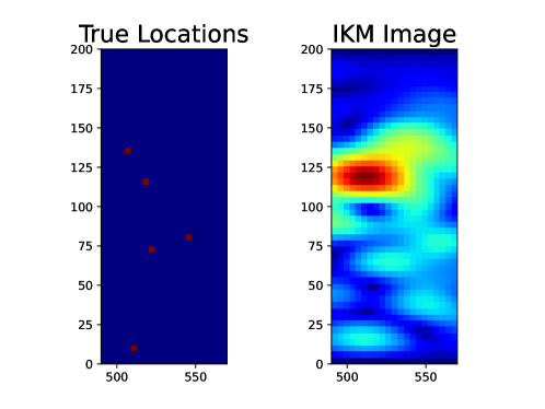
Figure 2: Left: True locations (left) and ${\mathcal{I}}^{\scriptscriptstyle{\rm KM}}$ image (right) of five point sources located at $\mbox{$\vec{\bi{x}}$}_{1}=(507,135)$ m, $\mbox{$\vec{\bi{x}}$}_{2}=(519,116)$ m, $\mbox{$\vec{\bi{x}}$}_{3}=(523,73)$ m, $\mbox{$\vec{\bi{x}}$}_{4}=(546,80)$ m and $\mbox{$\vec{\bi{x}}$}_{5}=(511,10)$ m, for $f_{c}=32.0625$ Hz, and $B=0.4f_{c}$ .

From the generated image, we observe that the imaging functional exhibits local maxima at the locations of the sources, but it struggles in discerning between the ones that are placed close to one another. This is a well-known limitation of such imaging methods, and is quantified by what is called the ‘resolution’ of the imaging functional. Performing a resolution analysis for any imaging functional, where we image a single point target, gives us an estimate of how close two targets can be in order for them to be well separated in the generated image. When using traditional imaging methods, the best resolution one can achieve is the Rayleigh limit of $\lambda/2$, where $\lambda$ is the wavelength of the frequency used to create the image. In the case of multiple frequency imaging, as the one shown in Figure 2, then resolution is tied to the wavelength of the central frequency $f_{c}$[17].

Linear imaging functionals such as (7) effectively regularize the ill-posed inverse source problem by implicitly assuming that the imaged object is a smooth low-pass function. Super-resolution (SR) is a body of mathematical and practical techniques which seek to overcome this limitation, by imposing different kinds of priors on the unknown object (in this context, the source distribution $g(\omega,\vec{x})$ in (1)). Classical SR methods assume small space-time object extent, in which case analytic continuation or singular function expansions can be used to extract information from the evanescent modes (recall (5)). However in such cases the number of degrees of freedom recovered beyond the Rayleigh limit scales only logarithmically with the signal-to-noise ratio [18, 19, 20, 21]. In recent years the sparse modeling methods have gained much popularity, both in general inverse problems [22] and more specifically in SR [23, 24]. These methods offer potentially much better accuracy and stability, at the expense of separation conditions, nonlinear reconstruction algorithms and complicated theoretical guarantees. Unfortunately, rigorous sparse SR techniques are nontrivial to generalize to wave-based imaging, and we are not aware of a theoretically solid and robust method for SR imaging even in this simple setup.

3 Deep Learning approach

In this section we describe the deep learning based method for the solution of the imaging problem elaborated in the previous section. In Section 3.1, we formulate the mathematical problem as a data-driven problem. In Section 3.2 we describe the DL architecture in detail, adding the physically-informed loss term in Section 3.3.

3.1 Data-driven formulation

In this section, we formulate the source refocusing problem as a data-driven problem. We create different scenarios that vary in the number of sources placed in the domain, as well as their locations. Each scenario is called a sample, and the number of sources and their locations in each sample are arbitrary. For each sample, a response matrix is created, as described in Section 2, which will be the input of the network. In more detail, the input for the network is the vector of measurements recorded in the sensors, per sample. Therefore, each of the $N_{samples}$ samples has the recorded data in each of the $N_{r}$ receivers $\{\mbox{$\vec{\bi{x}}$}_{r}\}_{r=1}^{N_{r}}$ for each of the $N_{f}$ frequencies $\{\mbox{$\omega$}_{j}\}_{j=1}^{N_{f}}$:

$$d_{q}=\{\Pi(\mbox{$\vec{\bi{x}}$}_{r};\mbox{$\omega$}_{j};q)\}_{r=1,\dots,N_{r}}^{j=1,\dots,N_{f}},\quad\Pi(\mbox{$\vec{\bi{x}}$}_{r};\mbox{$\omega$};q)=\sum_{i=1}^{N_{s}(q)}G(\mbox{$\vec{\bi{x}}$}_{r},\mbox{$\vec{\bi{x}}$}_{i,q};\mbox{$\omega$}),$$ (8)

where each source configuration $q=1,\dots,N_{samples}$ consists of $N_{s}(q)$ sources at locations $\mbox{$\vec{\bi{x}}$}_{i,q}$. The size of the input is therefore $N_{r}\times N_{f}$ for each sample.

Given an input $d\in\mathbb{C}^{N_{r}\times N_{f}}$, we would like the network to predict the source locations $\{\mbox{$\vec{\bi{x}}$}_{i}\}$. One possibility is to define the network output to contain the exact coordinates of these sources. However, in this case we have to fix the number of sources $N_{s}(q)=\textrm{const}$, since the network must have a constant sized output. We propose an alternative method, where the network should predict an image $\mathcal{I}=\mathcal{I}_{q}$ of dimension $N_{x}\times N_{y}$ corresponding to the source distribution $g$ as in (1), such that

$$\mathcal{I}_{q}=\bigvee_{i=1}^{N_{s}(q)}\mathfrak{P}(\mbox{$\vec{\bi{x}}$}_{i,q})$$ (9)

where $\mathfrak{P}(\mbox{$\vec{\bi{x}}$})$ stands for an $N_{p}\times N_{p}$ binary plateau centered at the location of the source a $\vec{\bi{x}}$, with the value $1$ inside the plateau region and $0$ everywhere else, and $\vee$ is the pixel-wise binary OR operation. These binary images are precisely the associated labels, being the desired outputs of the model that we use in the training phase (when training, the model fits input data to output labels).

The size of the output is therefore $N_{x}\times N_{y}$ for each sample. This method is popular in image segmentation problems and as we show later, turned out to be robust and effective in this context as well. On the flip side, we need to apply a post-processing method to infer the source locations from the predicted plateau images, as described in Section 4.3.

Choosing the plateau size $N_{p}$ turns out to be nontrivial as it incurs a tradeoff between stability and resolution. On the one hand, using a small number such as $N_{p}=1$ or $N_{p}=2$ creates sparse output images. From the experiments we observe that in those cases the network converges to the $0$ solution, in the sense that all the outputs of the network were $0$ images. This is due to the loss values being very low in that case (the $0$ solution is very close to the sparse output in terms of the loss function). Thus, the network returns the $0$ solution as a local minimum. On the other hand, when using large plateaus we obtain lower resolution in the sources refocusing, since it is harder to distinctly identify the sources due to a large overlap. In practice we choose $N_{p}$ by starting with $N_{p}=1$ and gradually increasing $N_{p}$ until the network no longer converges to the zero solution.

3.2 Deep-learning network architecture

As described in the previous section, the predictor network ${\cal NN}$ is a mapping

$${\cal NN}_{\theta}:\mathbb{C}^{N_{r}\times N_{f}} \to\left[0,1\right]^{N_{x}\times N_{y}},$$

$$d \mapsto\tilde{\mathcal{I}}(d;\theta),$$

where $d$ is the data image (8), $\tilde{\mathcal{I}}$ is the approximate binary plateau image (in fact, an image of probabilities, see below), and $\theta$ is a vector of weights whose values are found by the learning (training) process to be described below. The architecture of the network is schematically shown in Figure 3.

Figure 3: The architecture of the proposed Deep Learning network.

The network consists of a fully-connected (dense) layer which captures the global connections in the data, followed by a series of convolutional layers whose purpose is to capture local patterns, connected by the appropriate stacking and reshaping operations. We expect these local patterns to exist since two sources that are very close to each other will produce fields that are relatively similar, while the fields produced by sources that are far apart from each other will differ significantly. Similarly, the fields recorded by two close-by receivers will share a lot of characteristics, while if we, for example, compare recordings from two receivers on opposite ends of the array, we will find few to no similarities between them.

Effectively, the original 2D spatio-frequency image is converted to a 2D spatial output, and the convolutional filters facilitate the additional spatial dimension. In Figure 3, between the first and second row, we reshape the data from $N_{x}/N_{filters}\times N_{y}\times N_{filters}$ to $N_{x}\times N_{y}\times 1$, thereby transferring the information from the filters dimension into the spatial $x$ dimension. Each layer is followed by an activation function. We use a linear rectifier $x\rightarrow\max(0,x)$, while for the last layer we use the sigmoid function $x\rightarrow\frac{1}{1+e^{-x}}$ in order to obtain an image of probabilities (indeed, the sigmoid function is frequently used for segmentation problems).

The parameter vector $\theta$ consists of the weights $W_{i}$ and biases $b_{i}$ of the fully- connected layers $\sigma(A)_{i}=W_{i}A+b_{i}^{T}$, as well as the weights of the convolutional filters $w_{i}$ corresponding to the convolutional layers $\sigma(A)_{i}=w_{i}*A+b_{i}^{T}$.

The loss function we use for training the network, the target of the Stochastic Gradient Descent (SGD) algorithm, is the Negative Log-Likelihood (NLL) computed over the entire training set:

$$loss_{NLL}(\theta)\equiv\ell_{NLL}(\theta)=\frac{1}{N_{train}}\sum_{q=1}^{N_{train}}\ell_{CE}(\widetilde{\mathcal{I}}(d_{q};\theta),\mathcal{I}_{q}),$$ (10)

where $\{\mathcal{I}_{q}\}_{q=1}^{N_{train}}$ are the true train labels as defined in (9), and $\ell_{CE}$ is the pixel-wise cross-entropy loss

$$\ell_{CE}(\widetilde{\mathcal{I}},\mathcal{I})=-\frac{1}{N_{x}\cdot N_{y}}\sum_{i=1}^{N_{x}}\sum_{j=1}^{N_{y}}(\mathcal{I})_{i,j}\log(\widetilde{\mathcal{I}})_{i,j}.$$

Informally, the NLL loss approximates the total likelihood of pixels from the prediction to be of similar value as the ones in the true label. Minimizing $\ell_{CE}$ is equivalent to maximizing the overlap between the predicted plateaus and the true plateaus. Since $\tilde{\mathcal{I}}\neq 0$ (it is the output of the sigmoid function in the last layer), $\ell_{CE}$ (and therefore $\ell_{NLL}$) is clearly differentiable.

3.3 Physically Informed loss

We have found by experimentation (see Section 4) that the network trained with minimizing the $\ell_{NLL}$ loss was performing well on its own. However, the $NLL$ loss does not take into account any knowledge of the underlying physical problem. We implement a physically-informed loss term by using the true and the predicted images $\mathcal{I}$, $\tilde{\mathcal{I}}$ as (discretized) source functions in the Helmholtz equation, and comparing the pressure fields which would result from those sources in the search domain. By utilizing the physical knowledge of the problem, we expect better performance (e.g. convergence speed and accuracy) of the network.

In more detail, let $f(\mbox{$\vec{\bi{x}}$})$ and $\tilde{f}(\mbox{$\vec{\bi{x}}$})$ denote some functions $f,\tilde{f}:\mathcal{S}\to[0,1]$ such that $\mathcal{I},\tilde{\mathcal{I}}$ are precisely $f,\tilde{f}$ sampled on the $N_{x}\times N_{y}$ discretization ${\cal{S}}_{d}$ of the search domain $\mathcal{S}$. Considering these $f,\tilde{f}$ as extended sources, the solution of the corresponding Helmholtz equation can be written as

$$p(\mbox{$\omega$},\mbox{$\vec{\bi{x}}$})=\int_{\mathcal{S}}G(\mbox{$\vec{\bi{x}}$},\mbox{$\vec{\bi{y}}$};\mbox{$\omega$})f(\mbox{$\vec{\bi{y}}$})~{}\mathrm{d}\mbox{$\vec{\bi{y}}$},\qquad\tilde{p}(\mbox{$\omega$},\mbox{$\vec{\bi{x}}$})=\int_{\mathcal{S}}G(\mbox{$\vec{\bi{x}}$},\mbox{$\vec{\bi{y}}$};\mbox{$\omega$})\tilde{f}(\mbox{$\vec{\bi{y}}$})~{}\mathrm{d}\mbox{$\vec{\bi{y}}$},$$ (11)

where $G$ is the Green’s function as shown in eq. 5. Since $\tilde{f}$ is available only as the network output $\tilde{\mathcal{I}}(d;\theta)$, we compute an approximation to $\tilde{p}$ in any location $\mbox{$\vec{\bi{x}}$}\in\mathcal{S}$ by the quadrature formula

$$\tilde{p}(\mbox{$\omega$},\mbox{$\vec{\bi{x}}$})\approx\sum_{\mbox{$\vec{\bi{y}}$}_{j}\in{\cal{S}}_{d}}G(\mbox{$\vec{\bi{x}}$},\mbox{$\vec{\bi{y}}$}_{j};\mbox{$\omega$})\left(\tilde{\mathcal{I}}(d;\theta)\right)_{\mbox{$\vec{\bi{y}}$}_{j}}=:\tilde{V}(\mbox{$\vec{\bi{x}}$};d,\theta),\quad\mbox{$\vec{\bi{x}}$}\in\mathcal{S}.$$ (12)

For simplicity, we use the same method to approximate the true pressure field $p$ generated by the extended source $f$, i.e.

$$p(\mbox{$\omega$},\mbox{$\vec{\bi{x}}$})\approx\sum_{\mbox{$\vec{\bi{y}}$}_{j}\in{\cal{S}}_{d}}G(\mbox{$\vec{\bi{x}}$},\mbox{$\vec{\bi{y}}$}_{j};\mbox{$\omega$})\left(\mathcal{I}\right)_{\mbox{$\vec{\bi{y}}$}_{j}}=:V(\mbox{$\vec{\bi{x}}$};\mathcal{I}),\quad\mbox{$\vec{\bi{x}}$}\in\mathcal{S}.$$ (13)

Finally, using eq. 13 and eq. 12 we compute an approximation to the discrepancy between the pressure fields $p^{q},\tilde{p}^{q}$ (corresponding to the sources $\{\mbox{$\vec{\bi{x}}$}_{i,q}\}_{i=1}^{N_{q}}$) over the entire training set as

$$\ell_{PI}(\theta)=\frac{1}{N_{train}\cdot N_{x}N_{y}}\sqrt{\sum_{q=1}^{N_{train}}\sum_{\mbox{$\vec{\bi{x}}$}\in\mathcal{S}_{d}}\left|V(\mbox{$\vec{\bi{x}}$};\mathcal{I}_{q})-\tilde{V}(\mbox{$\vec{\bi{x}}$};d_{q},\theta)\right|^{2}}\approx\|p-\tilde{p}\|_{2}.$$

As we will see in the next section, this new physically-informed loss term helps the network converge to the desired solution more effectively. We train the network using both NLL and physically-informed loss term such that

$$loss_{PI}(\theta)=0.5\cdot\ell_{NLL}(\theta)+0.5\cdot\ell_{PI}(\theta)$$ (14)

and in this setup we achieved the best results. If one were to use only the PI term $\ell_{PI}$ as the loss function, the network would not converge. This is due to the random initialization of the weights, causing the outputs to be random as well. This “pure” PI loss, which is based on propagating a field generated by approximated sources, would saturate on a local minimum. On the other hand, the robustness of the NLL network allows us to generate accurate predictions of the sources, limited to the information in the data set. Using the knowledge of the underlying physical problem, the $\ell_{PI}$ term acts as a regularizer, penalizing the network on bad predictions. By combining $\ell_{NLL}$ and $\ell_{PI}$, we achieve the best performance. The choice of averaging the PI and NLL terms is justified by the fact that both losses are of the same order of magnitude.

4 Numerical Results

In this section, we present how the method performs and assess the effectiveness of the PI loss on the validation loss of the network.

4.1 Setup

We assume a homogeneous waveguide with constant wave speed $c_{0}=1500$ m/s and depth $D=200$ m. Homogeneous Dirichlet boundary conditions are applied on the top and bottom boundaries. The sources inside the waveguide emit signals across multiple frequencies and specifically have a central frequency $f_{c}=32.0625$ Hz and a bandwidth $B=0.4f_{c}$, i.e. the emitted frequencies are in the range $f\in\left[f_{c}-B/2,f_{c}+B/2\right]$. We uniformly discretize the frequency interval such that we use a total of $N_{f}=33$ frequencies. Furthermore, the vertical array is fixed at $x=0$ and spans the entire depth of the waveguide, with an inter-element distance of $h=2.5$ m, resulting in $N_{r}=81$.

We choose a search domain $\mathcal{S}=[490,570]\times[0,D]$ m, which we discretize with a square grid with $h_{x}=h_{y}=4$ m, thus $N_{x}=71$ and $N_{y}=51$. We generate $N_{samples}=5000$ samples, out of which $N_{train}=4050$ were used for training, 450 were used for validation, while the remaining 500 were used for testing. For each sample, the number of sources is randomly generated to be between 1 and 6, while their locations are also randomized per sample. Lastly, the network labels are created with an $N_{p}\times N_{p}$ plateaus around each source location as in eq. 9, with $N_{p}=3$.

4.2 Training

We trained the network using the stochastic gradient descent (SGD) algorithm ADAM [25], with 50 epochs and a batch size of $8$. We use the validation set to prevent the network from over-fitting the train data. If, during training, the computed loss over the training data continues to decrease and the computed loss over the validation data increases (using the same loss function), it means that the network is over-learning the training data and loses the ability to generalize to samples outside of the train data. Before we observe over-fitting, we terminate the training process.

4.3 Evaluation

To evaluate the performance of the trained network, we calculate the number of sources that the model located successfully out of all the sources in the testing data set. We first locate the sources in the output images by using a mean filter, where we replace each pixel value in an image with the mean value of its neighbors, including itself. This operation can be described by a convolution with a filter whose kernel is precisely $\frac{1}{N_{p}^{2}}\mathfrak{P}_{N_{p}}$ as in eq. 9.

An example of this evaluation process is shown in Figure 4. In the leftmost image, we plot the values of the approximates labels generated by the network for a single sample. In the middle plot, we show the effect of the mean filter in the image. We observe that this smoothed version of the image exhibits peaks in the locations of the point sources. From this, it is easy to recover the approximated locations of the sources, by simply thresholding the image for values close to 1. The result of this thresholding is shown in the rightmost plot, which shows the recovered approximate locations of the sources in this sample.

For each source, we check if the network managed to locate it precisely, by comparing it with the corresponding image that contains the true locations of each source in that sample. It is often sufficient to seek the source in a small area around the true location, however we chose to compare the exact locations, since in this case we are testing the resolution problem in the most challenging fashion.

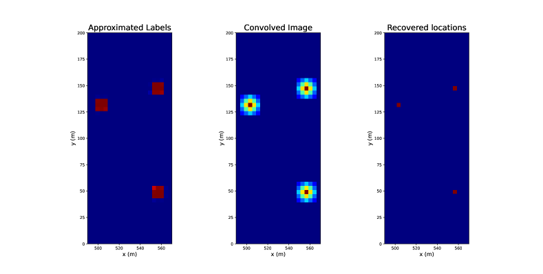
Figure 4: Approximated labels, generated by the network (left), Mean Filter version of the labels (middle) and recovered locations of the sources (right).

4.4 Results

In Figure 5 we present a visual example of the network output for the case where only the NLL loss $loss_{NLL}$ in (10) is used. In the first plot, we show the true locations of the sources we wish to image. In the second column we plot the modulus of the ${\mathcal{I}}^{\scriptscriptstyle{\rm KM}}$ image, given by eq. 7. The traditional imaging functional has trouble separating the sources effectively, as the resulting image focuses on the two rightmost sources that are also the ones closer together. Next, we plot the output of the network, i.e. the approximated labels. We see that while the approximate locations of the sources are recovered well, the overall image is distorted. Lastly, when trying to recover the exact locations of the sources, by using the evaluation method we just described. we can see that the network has managed to locate the two sources on the left that are well-separated, but did not manage to locate the sources that were placed closer to each other.

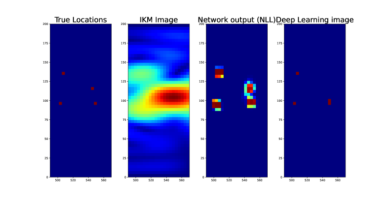
Figure 5: From left to right: True locations of the sources, ${\mathcal{I}}^{\scriptscriptstyle{\rm KM}}$ image, network output when only using the NLL loss.

Next, in Figure 6 we repeat the same experiment as in Figure 5, where we now use $loss_{PI}$ in (14) as the loss function during training. In the last two plots we see that the generated labels, plotted in the third column have vastly improved in quality. In the last plot, this translates to the perfect recovery of all the sources, including the two close-by sources that were place on the right.

Figure 6: From left to right: True locations of the sources, ${\mathcal{I}}^{\scriptscriptstyle{\rm KM}}$ image, network output when only using the physically-informed loss.

Having seen the qualitative improvement that the physically-informed loss offers to the model, we want to also examine its performance in a quantitative way. In Figure 7 we plot the validation loss of the network with respect to the epochs, and we observe that the validation loss corresponding to the usage of the physically-informed loss, represented by the yellow line, is immediately smaller than if that loss term was not used, represented by the blue line. Moreover, the recovery rate for the source locations starts at $59\%$ when using the NLL loss, but jumps to $75\%$ when using the physically-informed loss, thus showing the major contribution of the knowledge of the physical problem to the accuracy of the proposed method.

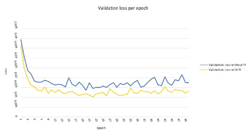
Figure 7: Validation loss per epoch, without the usage of the physically-informed loss term (blue) and with the implementation of the physically-informed loss term (yellow).

While Figure 7 clearly indicates the superior performance of the network when using the PI loss, we would still like to have more insight into the benefits of this situation. In Figure 8 we plot the recovery rates of the sources, with respect to the minimal distance of sources in each sample, i.e.

$$\min_{\begin{array}[]{c}\scriptstyle i,j=1,2,\ldots,N_{s},\\ \scriptstyle i\neq j\end{array}}\left|\mbox{$\vec{\bi{x}}$}_{i}-\mbox{$\vec{\bi{x}}$}_{j}\right|.$$

We see that the PI loss, plotted with a solid blue line, consistently outperforms the NLL loss, plotted with a dashed red line. It is of exceptional interest that the discrepancy between the two methods is the largest near the Rayleigh limit $\lambda_{c}/2$, plotted with a vertical dotted line. It is of great interest that in the super-resolution regime, where the minimum distance is below $\lambda_{c}/2$, the PI loss massively outperforms the NLL loss, with the difference in performance between the two methods becoming less significant as we move to higher minimum distances.

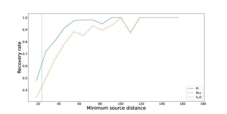
Figure 8: Recovery rates of sources, as a function of the minimum distance between sources per sample.

Finally, we examine the performance of our model in the presence of measurement noise. Specifically, we use the network trained on noiseless data, on test data which is contaminated by noise. The goal is to study how different levels of noise affect the ability of the model to recover the sources. Each clean test sample $d_{q}\in\mathbb{C}^{N_{r}\times N_{f}}$ as in (8) is modified as follows:

$$\tilde{d}_{q}(r,j)=d_{q}(r,j)+W_{q}(r,j),\quad r=1,\dots,N_{r},\;j=1,\dots,N_{f},$$ (15)

where $W_{q}(r,j)$ is chosen according to some distribution. Two noise distributions were tested: uniform and Gaussian.

To implement the uniformly distributed noise, we set for each $d_{q}$ in the test set (here $\mathcal{U}([a,b])$ denotes the uniform distribution over the interval $[a,b]$)

$$W_{q}(r,j) =\Re{d_{q}(r,j)}\cdot(1+w_{1,q}(r,j))+\imath\Im{d_{q}(r,j)}\cdot(1+w_{2,q}(r,j))$$

$$w_{1,q}(r,j),w_{2,q}(r,j) \sim\varepsilon\mathcal{U}([-1/2,1/2]),\quad r=1,\dots,N_{r},\;j=1,\dots,N_{f}.$$

Thus, both real and imaginary parts of the data are perturbed by uniform noise of relative magnitude $\varepsilon$. The performance of the network as a function of $\varepsilon$ is shown in Figure 9. The model is extremely stable both for the NLL and the PI loss.

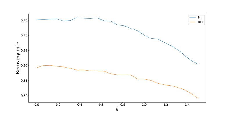
Figure 9: Recovery rates of sources with uniformly perturbed test data.

For the Gaussian noise, we follow [26]. For each test sample $d_{q}$ and $j=1,\ldots,N_{f}$, denote by $d_{q}^{(j)}$ the $j$-th column of the data matrix, corresponding to the measurements obtained by the entire receiver array at the frequency $\omega_{j}$. For $\varepsilon>0$, let $w_{q}^{(j)}\in\mathbb{C}^{N_{r}}$ be a zero mean uncorrelated Gaussian distributed vector with variance $\varepsilon p_{avg}$,  where

$$p_{avg}=\frac{1}{N_{r}}\left\|d_{q}^{(j)}\right\|^{2}_{2},$$

i.e. $w_{q}^{(j)}(r)\sim\mathcal{N}(0,\varepsilon p_{avg})$. Finally, the noise matrix in (15) is

$$W_{q}=[w_{q}^{(1)}\;\dots\;w_{q}^{(N_{r})}].$$

Thus, the expected power of the noise for the measurement at frequency $\omega_{j}$ over all the receivers is

$$\mathbb{E}\left[\left\|w_{q}^{(j)}\right\|^{2}_{2}\right]=\varepsilon N_{r}p_{avg},$$

while the total power of the signal recorded on all the receivers is $N_{r}p_{avg}$. Therefore, our Signal-to-Noise Ratio (SNR) in dB is given by $-10\log_{10}\varepsilon$.

In Figure 10, we plot the recovery rates of our model, under varying levels of Gaussian measurement noise. We have chosen $\varepsilon=10^{-4},10^{-3},10^{-2},0.1,1,10$, which correspond to SNR values of $40,30,20,10,0,-10$ dB respectively. As can be immediately seen, our model performs very well under the presence of noise, only losing accuracy for the first time at an SNR of 0 dB. For the sake of clarity, let us note here that a choice of $\varepsilon=1$, which corresponds to an SNR value of 0, the average power of the measurement noise is the same as the average power of the signal. Our last point at $-10$ dB sees a sharp drop in performance, but that is to be expected, as at this point the power of the noise far exceeds the power of the recorded signal.

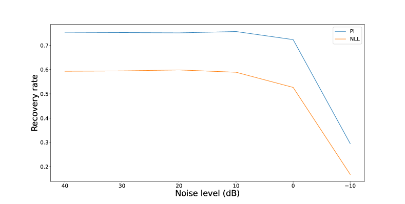
Figure 10: Recovery rates of sources with Gaussian noise.

5 Summary and conclusions

In this work we have demonstrated a successful deep learning method to waveguide imaging of multiple point sources, overcoming the Rayleigh resolution limit in practice. We have also shown that adding a physically informed loss term results in significant improvement in the accuracy of the network predictive power. Future work includes imaging in more complicated geometries, in particular where there is no known analytical solution (such as waveguides with variable depth, terminating and inhomogeneous waveguides), and a 3D implementation. Moreover, it will be interesting to compare the approach to other emerging DL methods to super-resolution, e.g. [27].

References

- [1] Uri Albocher, Assad A Oberai, Paul E Barbone, and Isaac Harari. Adjoint-weighted equation for inverse problems of incompressible plane-stress elasticity. Computer Methods in Applied Mechanics and Engineering, 198(30-32):2412–2420, 2009.
- [2] Paul E Barbone, Assad A Oberai, and Isaac Harari. Adjoint-weighted variational formulation for a direct computational solution of an inverse heat conduction problem. Inverse Problems, 23(6):2325, 2007.
- [3] David Colton and Rainer Kress. Inverse Acoustic and Electromagnetic Scattering Theory, volume 93 of Applied Mathematical Sciences. Springer New York, 2013.
- [4] Victor Isakov. Inverse Problems for Partial Differential Equations, volume 127 of Applied Mathematical Sciences. Springer New York, 1998.
- [5] Albert Tarantola. Inverse problem theory and methods for model parameter estimation. SIAM, 2005.
- [6] Curtis R Vogel. Computational methods for inverse problems. SIAM, 2002.
- [7] Rex V Allen. Automatic earthquake recognition and timing from single traces. Bulletin of the seismological society of America, 68(5):1521–1532, 1978.
- [8] M Baer and U Kradolfer. An automatic phase picker for local and teleseismic events. Bulletin of the Seismological Society of America, 77(4):1437–1445, 1987.
- [9] Ludger Küperkoch, Thomas Meier, J Lee, W Friederich, and EGELADOS Working Group. Automated determination of p-phase arrival times at regional and local distances using higher order statistics. Geophysical Journal International, 181(2):1159–1170, 2010.
- [10] Reinoud Sleeman and Torild Van Eck. Robust automatic p-phase picking: an on-line implementation in the analysis of broadband seismogram recordings. Physics of the earth and planetary interiors, 113(1-4):265–275, 1999.
- [11] Haiqiang Niu, Emma Reeves, and Peter Gerstoft. Source localization in an ocean waveguide using supervised machine learning. The Journal of the Acoustical Society of America, 142(3):1176–1188, 2017.
- [12] Maziar Raissi, Paris Perdikaris, and George E Karniadakis. Physics-informed neural networks: A deep learning framework for solving forward and inverse problems involving nonlinear partial differential equations. Journal of Computational physics, 378:686–707, 2019.
- [13] Weiqiang Zhu and Gregory C Beroza. Phasenet: a deep-neural-network-based seismic arrival-time picking method. Geophysical Journal International, 216(1):261–273, 2019.
- [14] Simon Arridge, Peter Maass, Ozan Öktem, and Carola-Bibiane Schönlieb. Solving inverse problems using data-driven models. Acta Numerica, 28:1–174, May 2019. Publisher: Cambridge University Press.
- [15] Atilim Gunes Baydin, Barak A Pearlmutter, Alexey Andreyevich Radul, and Jeffrey Mark Siskind. Automatic differentiation in machine learning: a survey. Journal of Marchine Learning Research, 18:1–43, 2018.
- [16] George Em Karniadakis, Ioannis G. Kevrekidis, Lu Lu, Paris Perdikaris, Sifan Wang, and Liu Yang. Physics-informed machine learning. Nature Reviews Physics, 3(6):422–440, June 2021.
- [17] Norman Bleistein. Mathematical methods for wave phenomena. Academic Press, 2012.
- [18] Dmitry Batenkov, Laurent Demanet, and Hrushikesh N Mhaskar. Stable soft extrapolation of entire functions. Inverse Problems, 35(1):015011, January 2019.
- [19] Mario Bertero and Christine de Mol. III Super-Resolution by Data Inversion. Progress in Optics, 36:129–178, January 1996.
- [20] Geoffrey De Villiers and E. Roy Pike. The Limits of Resolution. CRC Press, 2016.
- [21] Jari Lindberg. Mathematical concepts of optical superresolution. Journal of Optics, 14(8):083001, 2012.
- [22] Ingrid Daubechies, Michel Defrise, and Christine De Mol. Sparsity-enforcing regularisation and ISTA revisited. Inverse Problems, 32(10):104001, October 2016.
- [23] Emmanuel J. Candès and Carlos Fernandez-Granda. Towards a Mathematical Theory of Super-resolution. Communications on Pure and Applied Mathematics, 67(6):906–956, June 2014.
- [24] Dmitry Batenkov, Gil Goldman, and Yosef Yomdin. Super-resolution of near-colliding point sources. Information and Inference: A Journal of the IMA, 10(2):515–572, June 2021. Publisher: Oxford Academic.
- [25] Diederik P Kingma and Jimmy Ba. Adam: A method for stochastic optimization. arXiv preprint arXiv:1412.6980, 2014.
- [26] Liliana Borcea, George Papanicolaou, and Fernando Guevara Vasquez. Edge illumination and imaging of extended reflectors. SIAM Journal on Imaging Sciences, 1(1):75–114, 2008.
- [27] Matthew Li, Laurent Demanet, and Leonardo Zepeda-Núñez. Accurate and Robust Deep Learning Framework for Solving Wave-Based Inverse Problems in the Super-Resolution Regime. arXiv:2106.01143 [cs, math, stat], June 2021. arXiv: 2106.01143.