Enabling Efficient and General Analytics in Multidimensional Data Streams

Abstract.

Today’s large-scale services (e.g., video streaming platforms, data centers, sensor grids) need diverse real-time summary statistics across multiple subpopulations of multidimensional datasets. However, state-of-the-art frameworks do not offer general and accurate analytics in real time at reasonable costs. The root cause is the combinatorial explosion of data subpopulations and the diversity of summary statistics we need to monitor simultaneously. We present Hydra, an efficient framework for multidimensional analytics that presents a novel combination of using a “sketch of sketches” to avoid the overhead of monitoring exponentially-many subpopulations and universal sketching to ensure accurate estimates for multiple statistics. We build Hydra as an Apache Spark plugin and address practical system challenges to minimize overheads at scale. Across multiple real-world and synthetic multidimensional datasets, we show that Hydra can achieve robust error bounds and is an order of magnitude more efficient in terms of operational cost and memory footprint than existing frameworks (e.g., Spark, Druid) while ensuring interactive estimation times.

PVLDB Reference Format:
PVLDB, 15(11): 3249 - 3262, 2022.
doi:10.14778/3551793.3551867

PVLDB Artifact Availability:
The source code, data, and/or other artifacts have been made available at %leave␣empty␣if␣no␣availability␣url␣should␣be␣sethttps://github.com/antonis-m/HYDRA_VLDB.

1. Introduction

Many large-scale infrastructures (e.g., Internet services, sensor farms, datacenter monitoring) produce multidimensional data streams that are growing both in data volume and dimensionality (Bailis et al., 2017; Asta, 2016; Pelkonen et al., 2015; lin, 2015). These multidimensional data contain measurements of metrics along with metadata that describe said measurements across domain-specific dimensions. For instance, video streaming services analyze user experience issues across dimensions, such as ISP, CDN, Device, City, etc. (Jiang et al., 2013; Jiang et al., 2016). We see similar trends in other domains e.g., network and data center monitoring (aws, 2019, 2018; Liu et al., 2016).

In these settings, analysts need interactive and accurate estimates of diverse summary statistics across multiple data subpopulations of their data. For instance, video analysts want to monitor different statistics of viewer quality across subpopulations of viewers (e.g., entropy of bitrate in each major US city, etc.) (Jiang et al., 2016). Similarly, network operators want to analyze traffic grouped by combinations of their 5-tuple (srcIP, dstIP, srcPort, dstPort, protocol) (Liu et al., 2016). This is analogous to classical OLAP cube applications where the number of cube vertices grows exponentially as more subpopulations are admitted.

In such multidimensional telemetry settings, we ideally want frameworks offering high fidelity and interactive estimates at low operational cost. However, there are two fundamental challenges. First, there is a combinatorial explosion of data subpopulations to monitor, which can result in exponential overhead in operational costs and resources. Second, estimating multiple statistics entails compute and/or memory overhead proportional to the number of statistics of interest.

We find that existing frameworks are fundamentally limited in terms of the tradeoff across operational cost, accuracy, and estimation latencies they can offer. Exact analytics frameworks (e.g., Spark (Zaharia et al., 2016), Hive (Thusoo et al., 2009), Druid (Yang et al., 2014)) that rely on horizontal resource scaling entail poor cost-performance tradeoffs as datasets become larger. While approximate analytics (Chaudhuri et al., 2017) (e.g., sampling- or sketch-based analytics) can trade off estimation accuracy for lower cost and improved interactivity, these too suffer undesirable tradeoffs. For instance, sampling-based approaches provide generality across metrics and can handle many subpopulations, but their accuracy guarantees can be weak. On the other hand, sketch-based analytics (e.g., (Gan et al., 2018; Yu et al., 2013; Chen et al., 2020; Ting, 2019, 2018; Gan et al., 2020; Acharya et al., 1999; Agarwal et al., 2013a; Ben Basat et al., 2017; Basat et al., 2020, 2021)) can offer robust accuracy guarantees, but cannot address the combinatorial explosion of data subpopulations and also incur per-statistic effort.

In this paper, we present Hydra, a framework for efficient and general analytics over multidimensional data streams. Hydra builds on the novel combination of two key ideas. First, to tackle the combinatorial explosion of subpopulations, we use a “sketch of sketches” that enables memory efficient data stream summarization. This reduces the framework’s data-resident memory footprint by one to two orders of magnitude compared to Spark- and Druid-based alternatives and offers robust and provable accuracy guarantees. Second, to provide high-fidelity estimations simultaneously for many statistics, we leverage universal sketching (Liu et al., 2016). Unlike canonical sketch-based approaches that deploy one custom sketch type per statistic (Gan et al., 2018; Ting, 2019, 2018), a universal sketch estimates multiple different summary statistics with only one sketching instance.

To the best of our knowledge, Hydra is the first work to: (a) propose the combination of a sketch-of-sketches with universal sketching for the multidimensional telemetry problem. While some prior works have proposed the concept of a sketch-of-sketches, they do so for more narrow estimates of interest and do not demonstrate practical system implementations supporting a broad range of estimates (e.g., (Considine et al., 2009)); (b) analytically prove the theoretical guarantees of such a construction; and (c) design a practical end-to-end system design and implementation of this idea using the theoretical analysis. We build a prototype Hydra on Apache Spark but note that our core design is platform agnostic and can be ported to other streaming/batching systems as well (Yang et al., 2014; Shvachko et al., 2010; kaf, 2017). We also implement practical optimizations to mitigate compute bottlenecks to further reduce Hydra’s runtime and cost.

We evaluate Hydra using two real-world datasets; (1) a 2h-long, January 2019 CAIDA trace from the equinix-NYC vantage point (cai, 2021, 2019) and (2) an anonymized real-world trace of video QoE from a video analytics provider capturing the perceived QoE of viewers of a US-based content provider (con, 2022). To further evaluate the sensitivity of Hydra-sketch, we also leverage a synthetic multidimensional dataset drawn from a Zipf distribution with different parameter values (Gan et al., 2020; Ting, 2019).

We compare Hydra against six baselines: A native Spark-SQL implementation for exact analytics, a Spark-based implementation that uniformly samples incoming data, a sketch-based approach that allocates one universal sketch instance persubpopulation, VerdictDB (Park et al., 2018) (a sampling-based alternative) and two key-value based implementations (on Apache Spark and Druid) that pre-aggregate data at ingestion time and provide precisely accurate analytics .

Our evaluation shows that: (1) Hydra offers robust accuracy (mean error across statistics $\leq$5% with 90% probability) at 1/10 of the operational cost of exact analytics frameworks; (2) Hydra’s configuration heuristics ensure close to optimal accuracy-memory tradeoffs; (3) Hydra’s memory footprint scales sub-linearly with dataset size and number of data subpopulations. Combined with performance optimizations that improve end-to-end runtime by 45%, Hydra offers 7-20$\times$ better query latency than Spark- and Druid-based alternatives.

2. Background and Motivation

In this section, we present several motivating scenarios, introduce key aspects of multidimensional telemetry, and discuss the limitations of existing analytics frameworks.

2.1. Motivating Scenarios

Video Experience Monitoring:  To maintain their ad- and/or subscription-driven revenues, video providers need to detect issues that can degrade viewer experience. To that end, analysts first collect video session summaries (i.e., per viewer measurements of video quality) and use them to periodically (e.g., every minute) compute summary statistics of various video quality metrics. This allows them to monitor viewer experience across multiple subpopulations of viewers (Jiang et al., 2013; Jiang et al., 2016; sur, 2015). For instance, to track the entropy of bitrate and the L1 Norm of buffering ratio – a common indicator of streaming anomalies – for viewers in different cities, analysts may want to estimate the following query:

    SELECT City, Entropy(Bitrate), L1Norm(Buffering)
    FROM SessionSummaries
    GROUP BY City

Network Flow Monitoring:  Network operators commonly rely on control-plane telemetry frameworks (Cranor et al., 2003; Gupta et al., 2018) for tasks such as traffic engineering (Feldmann et al., 2001; Liu et al., 2016), attack and anomaly detection (Ramachandran et al., 2008) or forensics (Xie et al., 2005). These frameworks periodically monitor performance metrics (e.g., flow distributions, per-flow packet sizes, latency, etc.) across different subpopulations of flows, i.e., network flows grouped across combinations of packet header fields. For instance, the operator might want to track indicators of DDoS attacks as follows:

    SELECT dstIP, Cardinality(srcIP)
    FROM FlowTrace
    GROUP BY dstIP

These use cases share a problem structure that is characteristic of multidimensional telemetry. Queries that involve estimating many statistics across many data subpopulations appear in various settings, such as A/B testing (Johari et al., 2017; Hill et al., 2017), exploratory data analysis (Bailis et al., 2017; Vartak et al., 2015), operations monitoring (Abraham et al., 2013), and sensor deployments (Yang et al., 2020).

2.2. Requirements and Goals

Drawing on these use cases, we derive three key properties of the telemetry problem we want to tackle:

• Multidimensional Data: We define a multidimensional data record as $\mathit{x}=(\mathit{d}_{1},\dots,\ \mathit{d}_{\mathit{D}},\ \mathit{m})$, where $\mathit{d}_{\mathit{i}}$ is the value of a dimension $\mathit{D}_{\mathit{i}}$ and $\mathit{m}$ is the value of metric $\mathit{M}$. In video, quality metrics might be bitrate or buffering time whereas dimensions might be the viewer’s location, their player device, their ISP or CDN. Metrics and dimensions are domain- and usecase-specific.

• Analytics on Data Subpopulations: Analytics are estimated in parallel across subpopulations of the input data. A subpopulation $\mathit{Q}_{\mathit{i}}$ is a collection of data records $\{\mathit{x}_{i}\}$ such that all $\mathit{x}_{i}\in\mathit{Q}_{\mathit{i}}$ match on a subset of dimension values. With a slight abuse of notation, we define $\mathit{Q}_{\mathit{i}}$ using this set of dimension values, i.e., $\mathit{Q}_{\mathit{i}}=\{\mathit{D}_{\mathit{i},1}=\mathit{d}_{\mathit{i},1}\land\dots\land\mathit{D}_{\mathit{i},\mathit{l}}=\mathit{d}_{\mathit{i},\mathit{l}}\}$, where $\{\mathit{D}_{\mathit{i},1},\dots,\mathit{D}_{\mathit{i},\mathit{l}}\}\subseteq\{\mathit{D}_{1},\dots,\mathit{D}_{\mathit{D}}\}$; e.g., a data subpopulation could be NYC-based viewers using AppleTV.

• Multiple statistics to estimate: For each subpopulation, the operator wants to estimate various summary statistics e.g., heavy hitters, entropy, cardinality, etc. A query $\mathit{q}_{\mathit{k}}$ specifies a set of subpopulations $\{\mathit{Q}_{\mathit{i}}\}$ and a statistic $\mathit{g}$ to estimate using the values $\mathit{m}_{\mathit{j}}$ of $\mathit{x}_{\mathit{j}}\in\mathit{Q}_{\mathit{i}}$.

In practice, operators have three requirements: (1) High fidelity for a broad set of statistics i.e., robust, apriori configured, error bounds for as many statistics as possible; (2) Near real-time estimations and; (3) Low footprint (e.g., cloud compute and memory costs).

2.3. Prior Work and Limitations

Prior work has focused on developing two broad (but not mutually exclusive) approaches for multidimensional telemetry. The first enables distributed computations by horizontally scaling the frameworks’ resources. The second enables approximate analytics that sacrifice estimation accuracy for improved performance.

• Horizontal resource scaling:  Here we find SQL and NoSQL analytics frameworks whose distributed design reduces estimation latency through horizontal scaling of server resources (e.g., Spark (Zaharia et al., 2016), Hive (Thusoo et al., 2009), Hadoop (Shvachko et al., 2010), Dremel (Melnik et al., 2010), Druid (Yang et al., 2014), Flink (Carbone et al., 2015)). These frameworks scale their clusters with input data and can provide precisely exact estimations. However, as data volume and dimensionality grow, i) deploying such clusters becomes increasingly expensive and ii) the continuous addition of resources eventually results in marginal estimation latency gains due to data shuffling overheads (Agarwal et al., 2013b).

• Approximate Analytics:  Approximate analytics frameworks leverage sampling or data summarization algorithms in order to trade off accuracy for performance and cost. Sampling-based frameworks allow for low estimation latency by sampling data either online, at query time (the analyst applies the sampling operators and parameters as part of the estimation query) (Armbrust et al., 2015; Chaiken et al., 2008; Melnik et al., 2010; Olston et al., 2008; Thusoo et al., 2009) or offline, by means of a pre-processing step that creates data samples to be used at query time (Agarwal et al., 2013b; Acharya et al., 2000; Acharya et al., 1999; Sidirourgos et al., 2011).

  While there is a rich body of sampling-based efforts, these have two key shortcomings. First, their accuracy guarantees are in the form of confidence bounds that are computed after query estimation has taken place and that depend on the statistic being estimated and the number of samples used (Ma and Triantafillou, 2019). Therefore, when an estimate does not meet accuracy requirements, frameworks often fall back to using other samplers or precisely exact estimates. Second, to offset the resource overheads of producing offline samples, frameworks often make hard apriori choices on what subsets of their data to create samples for (e.g., BlinkDB (Agarwal et al., 2013b) that mines query logs for frequently queried data or VerdictDB (Park et al., 2018) that allows users to identify popular data tables). In contrast, sketch-based analytics ensure bounded accuracy-memory trade-offs for arbitrary workloads in sub-linear space (Cormode et al., 2012; Cormode and Muthukrishnan, 2005; Durand and Flajolet, 2003; Liu et al., 2016; Yu et al., 2013). These frameworks build compact data summaries at ingestion and use them to estimate statistics with apriori provable error bounds.

We can also combine horizontal resource scaling and approximations. For instance, both Apache Spark and Druid allow for data summarization at ingestion time such that incoming data are stored as a key-value store where the keys are distinct $\langle\mathit{Q}_{\mathit{i}},\ \mathit{m}_{j}\rangle$ tuples and the values are their respective counts. These hybrid approaches enable data reduction without compromising the framework’s ability to offer precise estimations.

Qualitative Analysis:  Next, we analyze the overhead to process multidimensional streams and the resident data cost using the above solutions. Let us denote the dataset size (in terms of the number of data records) as $\mathit{V}$ and let $Q$ be the number of data subpopulations. Assuming $\mathit{D}$ dimensions and that each data record belongs in $2^{\mathit{D}}$ different subpopulations, then $Q=\mathcal{O}(2^{\mathit{D}}\times\mathit{V})$. In practice, assuming each dimension has cardinality $\mathit{C}$, there are $\mathcal{O}(\mathit{C}^{\mathit{D}})$ subpopulations in the dataset. In practice, we find that $\mathcal{O}(2^{\mathit{D}}\times\mathit{V})$ is a tighter empirical bound for $Q$ and we will use that moving forward. In addition, given that the framework needs to estimate $\mathcal{O}(\mathit{S})$ different statistics, the number of summary statistics to be estimated is an exponential $\mathcal{O}(\mathit{Q}\times\mathit{S})=\mathcal{O}(2^{\mathit{D}}\times\mathit{V}\times\mathit{S})$. Assuming, as it is the case for frameworks for precisely exact analytics, that the CPU and memory requirements for data ingestion and/or statistics estimation scale linearly with subpopulations, we see that the framework’s runtime, resource requirements and cost also scale exponentially.

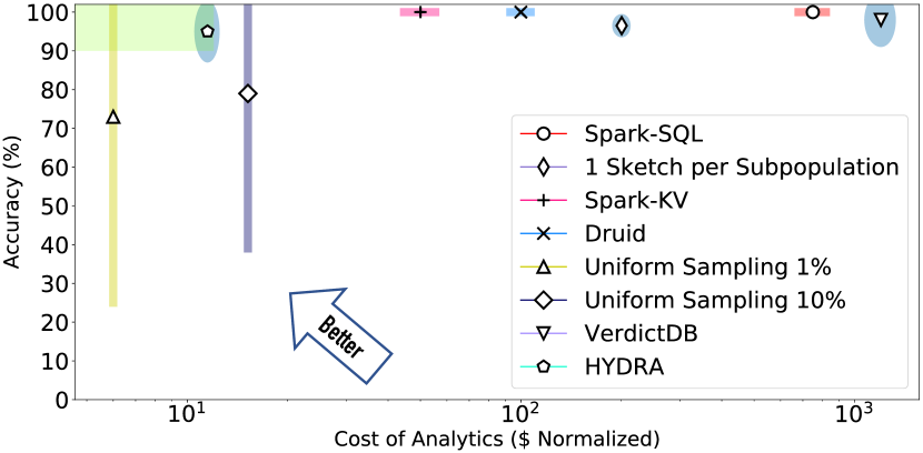
Figure 1. End-to-end cost of analytics. The green-shaded region indicates the ideal operating regime for Hydra.

Quantitative Analysis:  To corroborate this qualitative analysis, we evaluate the operational cost for several analytics frameworks when used in a multidimensional context (Figure 1). Specifically, we measure their $ cost as a function of their observed accuracy when asked to estimate in real-time 4 summary statistics from a 130GB real-world dataset with approximately 5.6 million data subpopulations. Following the typical cloud billing model (pri, 2022), we use the total runtime $\times$ the number of cluster nodes used (20) as a proxy for the $ cost. We provide a detailed description of our experimental setup and baselines in §6. Ideally, we need a framework whose cost-accuracy tradeoff lies in the top-left, green region, i.e., it offers the accuracy of a precise analytics framework at the cost of sampling. However, we observe that the cost gap between the cheapest (1% uniform sampling) and the most expensive baselines (precisely accurate Spark-SQL) is two orders of magnitude wide. A sketch-based approach where the framework allocates one sketch per subpopulation, while cheaper than Spark-SQL, remains expensive as it allocates exponentially many sketch instances, thus incurring high memory overheads. As discussed in §6, this baseline uses universal sketching that can simultaneously estimate all 4 statistics of interest per subpopulation with one sketch. Finally, precise baselines that summarize data at ingestion time, such as Apache Druid and Spark (denoted as Spark-KV) lie in the middle between Spark-SQL and sampling.

Key takeaways:  Multidimensional telemetry entails a combinatorial explosion of data subpopulations and summary statistics to monitor. Balancing cost, accuracy, and estimation latency is challenging due to the combinatorial explosion in data subpopulations and the number of summary statistics the framework needs to enable. Existing frameworks can only meet a subset of these goals, which motivates us to rethink how to support such analytics workloads at scale.

3. Hydra: System Overview

To support multidimensional workloads at scale, we envision Hydra as a streaming, sketch-based OLAP framework (Yang et al., 2014; ola, 2016). Hydra’s distributed design (illustrated in Figure 2) includes one frontend and multiple worker nodes and its input are i) streams of multi-dimensional data, ingested in parallel at the worker nodes and ii) estimation queries provided by the operator to the frontend node. Hydra implements two logical operations: Data Ingestion and Query Estimation.

1. Data Ingestion: Data Ingestion happens at the worker nodes. Each worker summarizes an incoming data stream to a local instance of Hydra-sketch. Data summarization happens on a per-subpopulation basis. Specifically, for every incoming data record, Hydra first identifies what subpopulations the data record belongs in and correspondingly updates a novel sketching primitive that we discuss below, Hydra-sketch. Hydra-sketch instances are configured to ensure accuracy guarantees and low memory footprint (§4.6).

2. Query Estimation: Query Estimation involves both frontend and worker nodes. The frontend receives operators’ queries with i) the statistics to estimate and ii) the set of subpopulations to estimate these statistics on. Using this information, it creates a query plan that is distributed to the worker nodes who execute the queries. After estimation has taken place, the frontend node collects the results from the workers and returns them to the operator.

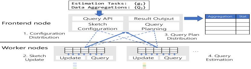
Figure 2. Hydra’s example workflow. Workers perform data ingestion and querying. The frontend node exposes the query API to the operator and performs configuration and query plan dissemination.

While the idea of using sketching to optimize analytics is not new, in our context canonical sketch-based approaches will need to instantiate up to $\mathcal{O}(\mathit{S})$ sketch instances per subpopulation. This is inefficient as the framework needs exponentially many sketch instances, despite a sketch’s ability to summarize a subpopulation’s data in sub-linear space.

Key Idea:  To avoid the above limitations of conventional approaches, Hydra uses a novel combination of two ideas.

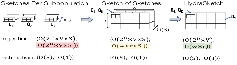
Figure 3. Comparison of Ingestion and Estimation (CPU time, space complexity) for different sketch-based designs. We highlight the theoretical improvements in space complexity from Hydra’s design ideas.

First, we observe that we can reduce the exponential $\mathcal{O}(\mathit{Q})=\ \mathcal{O}(2^{\mathit{D}}\times\mathit{V})$ ingestion-time, memory cost of sketch-based approaches through a novel “sketch of sketches”. We show that through a $\mathit{w}\times\mathit{r}$ array of sketch instances (Fig. 3), where $\mathit{w}\times\mathit{r}\ll 2^{\mathit{D}}\times\mathit{V}$, Hydra reduces the memory cost of estimating $\mathcal{O}(\mathit{S})$ statistics from $\mathcal{O}(2^{\mathit{D}}\times\mathit{V}\times S)$ to $\mathcal{O}(\mathit{w}\times\mathit{r}\times\mathit{S})$. The intuition is that, unlike canonical sketch-based approaches, we can summarize multiple subpopulations into one sketch instance and then query it with predictable error (Considine et al., 2009; Ting, 2019).

Second, to reduce the need for instantiating $\mathcal{O}(\mathit{S})$ different sketch types for $\mathcal{O}(\mathit{S})$ summary statistics, Hydra leverages universal sketching (Liu et al., 2016; Braverman and Ostrovsky, 2010). Universal sketching enables replacing $\mathcal{O}(\mathit{S})$ sketches with a single sketch that simultaneously estimates multiple different statistics per subpopulation. This means that as long the desired statistics can be estimated with a universal sketch, there is no limit in the number of statistics that the sketch can estimate with a fixed memory footprint. This design choice further reduces the framework’s space complexity from $\mathcal{O}(\mathit{w}\times\mathit{r}\times\mathit{S})$ to $\mathcal{O}(\mathit{w}\times\mathit{r})$.

While these two ideas (sketch of sketches and universal sketching) have been independently proposed in other narrower contexts, to the best of our knowledge, we are the first effort to: (1) propose the combination of these ideas to tackle the multidimensional telemetry problem; (2) rigorously prove the accuracy-resource tradeoffs of this construction; and (3) demonstrate a practical end-to-end realization atop state-of-art horizontally scalable “BigData” platforms.

4. Hydra Detailed Design

We first provide background on sketching to set up the intuition for Hydra-sketch. We then introduce the basic Hydra-sketch algorithm, formally prove its error bounds, and devise Hydra-sketch configuration strategies. Table 1 summarizes the notation we use.

Table 1. Hydra Notation. The upper subsection introduces notation specific to the sketch-of-sketches and the lower to universal sketches.

Notation	Definition
$\mathit{V}$	Input size
$\mathit{D}$	Number of data dimensions
$Q$	Number of data subpopulations
$\mathit{S}$	Number of summary statistics
$\mathbb{S}_{\mathit{m},\mathit{n}}$	Stream of length $\mathit{m}$ and $\mathit{n}$ distinct keys
$\mathit{w}$	Number of sketches per 2D-sketch row
$\mathit{r}$	Number of rows in 2D-sketch
$(\epsilon,\delta)$	$0<\epsilon<1$ as additive error and $\delta$ is the probability that
	the result error is not bounded by $\epsilon$ (failure probability)
$\mathit{w}_{\mathit{US}}$	Number of counters per universal sketch row
$\mathit{r}_{\mathit{US}}$	Number of universal sketch rows
$(\epsilon_{\mathit{US}},\delta_{\mathit{US}})$	$0<\epsilon_{\mathit{US}}<1$ as additive error in universal sketch and
	$\delta_{\mathit{US}}$ is the failure probability
$\mathit{L}$	Number of universal sketch layers
$\mathit{k}$	Number of keys in universal sketch heavy hitter heaps

4.1. Background on Sketching

Let $\mathbb{S}_{\mathit{m},\mathit{n}}$ denote a data stream with length $\mathit{m}$ and $\mathit{n}$ distinct keys. Suppose we want to estimate a frequency-based summary statistic of the keys (e.g., entropy, cardinality, frequency moments). A natural design is to estimate the desired statistic with a key-value data structure tracking the frequency per key. For instance, for frequency estimation, we can maintain and increment one counter per key. While correct, the space complexity is linear in $\mathit{n}$ and not space efficient (Figure 4).

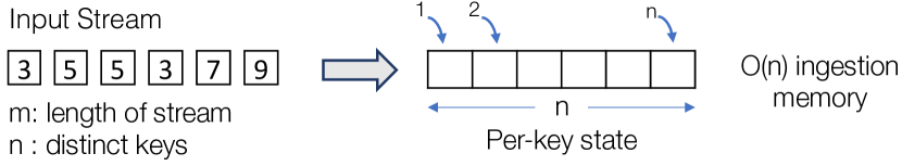
Figure 4. Maintaining per-key state is not space efficient

Hash-based mappings for space efficiency:  To ensure sub-linear (in $\mathit{n}$) space complexity, sketching algorithms do not maintain per-key state but, instead, map multiple keys to the same counters via hashing. For instance, a simple sketch for frequency estimation consists of $\mathit{w}$ integer counters, where $\mathit{w}\ll\mathit{n}$. Based on the hash of the key, an element gets mapped to a counter, which is then incremented to maintain an estimate of that key’s frequency. Naturally, multiple keys colliding introduces some errors (Figure 5).

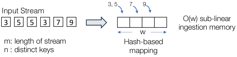
Figure 5. Hashing enables sub-linear memory complexity

Multiple independent updates for tighter error bounds:  As defined, this basic mechanism only provides a small probability that the estimation error will lie within a desirable range of error values (Alon et al., 1996). To overcome this, sketches use independent instances (e.g., $\mathit{r}$ arrays) of the counter structure of length $\mathit{w}$. Each vector of length $\mathit{w}$ has its own hash function and the $\mathit{w}$ hash functions are pairwise independent. Thus, ingesting a stream element now translates to $\mathit{r}$ update operations (e.g., incrementing $\mathit{r}$ integer counters instead of one). For each key, this sketch produces $\mathit{r}$ different estimates of the statistic of interest. The final estimate will be a summary of $\mathit{r}$ estimates (i.e., min, median etc.) (Figure 6) (Cormode et al., 2012). This amplifies the probability that the estimation error lies within the desired range.

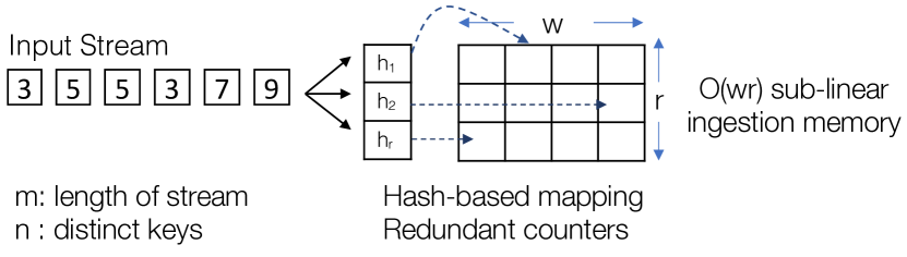
Figure 6. Independent hashing improves accuracy.

4.2. Tackling Subpopulation Explosion

For now, let us make the simplifying assumption (which we relax later) that our system only needs to estimate one summary statistic (e.g., entropy) per data subpopulation. Similar to Figure 4, a starting point for our design would be to maintain per-subpopulation state, i.e., allocate one sketch instance for each of the $\mathcal{O}(2^{\mathit{D}}\times\mathit{V})$ distinct subpopulations. This approach, similar to an OLAP cube, is not scalable as it requires as many sketches as the number of data subpopulations.

To avoid keeping per-subpopulation state, we borrow from the first intuition that we saw in the sketch construction in the background (Figure 5). The basic sketch construction avoids maintaining per-key state by allowing multiple keys to explicitly collide in a hashed key-value store whose size is less than the number of unique elements.

Note that the basic sketch is maintaining a single counter per array entry but we want to be able to estimate some statistical summary of a subpopulation instead. Therefore, instead of keeping a single counter per array entry, we maintain a sketch-per-entry. This brings us to the following construction (Figure 7). We consider a single array of $\mathit{w}$ (e.g., $\mathit{w}\ll 2^{\mathit{D}}\times\mathit{V}$) sketches. For each ($\mathit{Q}_{i}$, $\mathit{m}_{j}$) pair, we hash the $\mathit{Q}_{i}$ and map it to one of the $\mathit{w}$ sketches, thus colliding multiple subpopulations to the same sketch. Then, we update the sketch with $\mathit{m}_{j}$ and at query time, we estimate the statistic for $\mathit{Q}_{i}$.

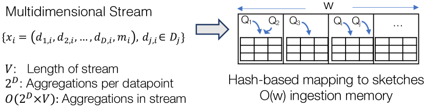
Figure 7. Hash-based mapping of subpopulations to a sketch vector.

Analogous to the basic sketch from §4.1, by mapping multiple subpopulations to one sketch, this baseline construction will have some estimation error. To control this, we extend the idea of using redundant counter vectors and pairwise-independent hashes (Figure 6). That is, we use $\mathit{r}$ arrays of $\mathit{w}$ sketches and use $\mathit{r}$ pairwise-independent hash functions to map each subpopulation to one sketch per row (Figure 8). At query time, we return the median of the $\mathit{r}$ estimates.

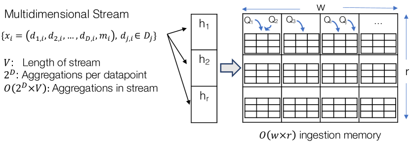
Figure 8. Redundant sketch vectors and pairwise-independent hashes for tighter error bounds.

In summary, the above sketch-of-sketch construction maintains a 2D array of sketches to track multiple subpopulations. This reduces the memory cost of ingestion to $O(\mathit{w}\times\mathit{r})$ i.e., sub-linear in subpopulations. In §4.5, we formally prove the memory-accuracy tradeoffs for this construction.

4.3. Enabling Multiple Statistics

The above discussion is based on the simplifying assumption that we need to only estimate one summary statistic. Since sketching algorithms are generally custom designed per statistic, to support $O(\mathit{S})$ different summary statistics, we need to create $O(\mathit{S})$ sketch-of-sketches instances. This raises two natural concerns. First, the total memory cost of this solution becomes $O(\mathit{w}\times\mathit{r}\times\mathit{S})$, i.e., linear to the number of summary statistics of interest. Second, the framework cannot offer generality as it cannot estimate summary statistics that are not already allocated; e.g., some future analysis might require estimating the entropy of a metric but the framework has not instantiated an entropy-specific sketch-of-sketch instance.

Our insight here is that the sketch of sketches structure can be combined with universal sketching (Liu et al., 2016) to achieve the desired generality across statistics. A universal sketch is a sketching primitive that enables the simultaneous estimation of multiple different, apriori unknown, statistics with one sketch instance. Therefore, instead of a sketch-of-sketches per statistic, we can use one sketch of universal sketches. We formally prove this in §4.5 and show that Hydra’s ingestion cost drops to $\mathcal{O}(\mathit{w}\times\mathit{r})$.

Background on universal sketches:  A universal sketch can estimate any summary statistic that belongs to a broad class of functions, known as Stream-PolyLog (Braverman and Chestnut, 2014; Braverman and Ostrovsky, 2010; Liu et al., 2016). We denote each function in Stream-PolyLog, as $\mathit{G}\text{-sum}=\sum{\mathit{g}(\mathit{f}_{\mathit{j}})}$, where $\mathit{f}_{\mathit{j}}$ is the frequency of the $\mathit{j}$-th unique element in the input stream $\mathbb{S}_{\mathit{m},\mathit{n}}$ and $\mathit{g}$ is a function defined over $\mathit{f}_{\mathit{j}}$. If $\mathit{g}$ is monotonically increasing and upper bounded by $\mathcal{O}({\mathit{f}_{\mathit{j}}}^{2})$, then $\mathit{G}\text{-sum}$ can be computed by a single universal sketch with polylogarithmic memory. Universal sketch provides $\epsilon$-additive error guarantees to Stream-PolyLog and demonstrates better memory-accuracy tradeoffs than the composition of custom sketches when estimating multiple statistics from Stream-PolyLog in practice (Liu et al., 2016). Key statistics of interest can be formulated via a suitable $\mathit{G}$-sum $\in$ Stream-PolyLog. Such examples include: $\alpha$-Heavy Hitters ($f_{i}\geq\alpha\Sigma f_{i}$), L1-Norm ($\Sigma f_{i}$), L2-Norm ($\Sigma f_{i}^{2}$) Entropy ($-\Sigma{\frac{f_{i}}{L_{1}}\text{log}\frac{f_{i}}{L_{1}}}$), and Cardinality ($|\langle f_{1},\dots,f_{N}\rangle|$). Note that there are many other summary statistics that can be estimated by combining statistics, such as standard deviation, histograms, mean, or median. A statistic that cannot be directly estimated by Hydra-sketch is quantiles.

The basic building block of universal sketches are L2-Heavy Hitter (HH) sketches e.g., Count-sketch (Minton and Price, 2014). Each count-sketch maintains $\mathit{r}_{\mathit{CS}}$ arrays of $\mathit{w}_{\mathit{CS}}$ counters each, $\mathit{r}_{\mathit{CS}}$ pairwise-independent hash functions and a max-heap keeping track of the top-$k$ Heavy Hitters in the sketch; When updating each count-sketch with a new data item, the sketch updates a randomly located counter in every row based on the corresponding hash index to keep track of that data item’s frequency. The top-$k$ HH heap is subsequently updated to reflect the addition of the new item. A universal sketch consists of $\mathit{L}$ layers of count-sketches. Each count sketch applies an independent 0-1 hash function $\mathit{h}_{\mathit{l}\in[0,\ \mathit{L})}$ to the input data stream to sub-sample at every layer (from the previous layer). These layers then track the heavy hitters, i.e., the important contributors to the $\mathit{G}$-sum.

The intuition here is that the layered structure of the universal sketch is designed for sampling representative elements with diverse frequencies, and these elements can be used to estimate $\mathit{G}$-sum with bounded errors. If only one layer of heavy hitter sketch were used, the estimations would lack representatives from less frequent elements. The heavy-hitters at each layer are processed iteratively from the bottom layer to the top and the recursively aggregated result is used to compute the desired statistic. This is an unbiased estimator of $\mathit{G}$-sum with bounded additive errors (Theorem 1).

Theorem 1 ((Liu et al., 2016; Braverman and Ostrovsky, 2010)).

Given a stream $\mathbb{S}_{\mathit{m},\mathit{n}}$ let us consider a Universal Sketch $\mathit{US}$ with $\mathit{L}=\mathcal{O}(\log\mathit{n})$ layers. If each layer of $\mathit{US}$ provides an $(\epsilon_{\mathit{US}},\ \delta_{\mathit{US}})$-L2 error guarantee, then $\mathit{US}$ can estimate any $\mathit{G}$-sum function $\mathit{G}\in\text{Stream-Polylog}$ to within a $(1\pm\epsilon_{\mathit{US}})$ factor with probability $1-\delta_{\mathit{US}}$. Satisfying a $(\epsilon_{\mathit{US}},\ \delta_{\mathit{US}})$-L2 error guarantee requires $O(log\mathit{n})$ Count-Sketch instances with $w_{\mathit{CS}}=\mathcal{O}(\epsilon_{\mathit{US}}^{-2})$ columns and $r_{\mathit{CS}}=\mathcal{O}(\log\delta_{\mathit{US}}^{-1})$ rows.

4.4. The Hydra-sketch Algorithm

Combining these ideas gives us the Hydra-sketch algorithm.

1. Updating Hydra-sketch: Updating Hydra-sketch with a data record, $\mathit{x}_{\mathit{j}}=<\mathit{d}_{1,\mathit{j}},\ \mathit{d}_{2,\mathit{j}},\ \dots,\mathit{d}_{\mathit{D},\mathit{j},},\ \mathit{m}_{\mathit{j}}>$ is a three-step process. At the first, “fan-out” stage, we compute the $O(2^{\mathit{D}})$ subpopulations $\{\mathit{Q}_{1},\dots,\mathit{Q}_{2^{\mathit{D}}}\}$ that $\mathit{x}_{\mathit{j}}$ belongs in. Note that while $O(2^{\mathit{D}})$ is an exponential term, it is exponential to the number of dimensions $\mathit{D}$ and, thus, significantly smaller than the total number of subpopulations $\mathit{Q}$, which is exponential to the cardinality of values in each dimension. Then, we map each $\mathit{Q}_{\mathit{i}}$ to $\mathit{r}$ universal sketches instances using $\mathit{r}$ pairwise-independent hash functions $\mathit{h}_{\mathit{k}\in[0,\mathit{r})}:\mathit{Q}_{\mathit{i}}\rightarrow[0,\mathit{w})$. For the $\mathit{k}^{th}$ row, the index of the universal sketch to update $\mathit{US}_{\mathit{k}}$ is the hash of $\mathit{Q}_{\mathit{i}}$ using hash function $\mathit{h}_{\mathit{k}}$. Last, we update each $\mathit{US}_{\mathit{k}}$ with the metric value $\mathit{m}_{j}$.

2. Querying Hydra-sketch: Hydra-sketch’s querying algorithm takes as input a statistic $\mathit{g}$ and an aggregation $\mathit{Q}_{\mathit{i}}$ i.e., the aggregation to estimate $\mathit{g}$ on. Querying consists of 2 steps. The first involves identifying the set of $\mathit{r}$ universal sketch instances $\{\mathit{US}_{\mathit{k}}\}$ that $\mathit{Q}_{\mathit{i}}$ maps to. Then $\mathit{g}$ is estimated from each $\mathit{US}_{\mathit{k}}$, and the median value of these estimations is returned.

Given this basic algorithm, we now focus on formally proving that Hydra-sketch offers rigorous accuracy guarantees and that it is usable in practice.

4.5. Accuracy Guarantees

Theorem 2 states the accuracy bounds of Hydra-sketch.

Theorem 2.

Let us assume that each Universal Sketch $\mathit{US}$ can approximate the $\mathit{G}$-sum, for a monotone function $g$ within a $(1+\epsilon_{\mathit{US}})$-factor with probability $1-\delta_{\mathit{US}}>1/2$. Further, let $\mathit{G}_{\mathbb{S}}$ be the $\mathit{G}$-sum applied to the stream $\mathbb{S}$ and $\mathit{G}_{i}$ when applied to the target subpopulation $\mathcal{\mathit{Q}}_{i}$. Then Hydra-sketch with $w=\mathcal{O}(\epsilon^{-1})$ columns and $r=\mathcal{O}(\log\delta^{-1})$ rows, for user defined parameters $\epsilon,\ \delta$, provides an estimate $\widehat{\mathit{G}_{i}}$ that with probability $1-\delta$ satisfies:

(1) $$\mathit{G}_{i}(1-\epsilon_{\mathit{US}})\leq\widehat{\mathit{G}_{i}}\leq\mathit{G}_{i}(1+\epsilon_{\mathit{US}})+\epsilon\cdot\mathit{G}_{\mathbb{S}}$$

Proof.

To bound the error of our algorithm, we analyze the frequency vector $f_{j}$ of the stream of elements mapped to each Universal Sketch instance $\mathit{US}_{j}=\mathit{h}_{j}(\mathit{Q}_{i})$, where $\mathit{Q}_{i}$ is the queried subpopulation. The frequencies of all $\mathit{m}_{i}\in\mathit{Q}_{i}$ are guaranteed to appear in $f_{j}$, since the Update algorithm of §4.4 maps them to $\mathit{US}_{j}$.

Let $\mathfrak{Q}=\left\{\mathit{Q}_{1},\ldots,\right\}$ denote all groups in the input stream $\mathbb{S}$, and let $\mathfrak{Q}_{j}=\left\{\mathit{Q}_{k}\in\mathfrak{Q}\mid\mathit{h}_{j}(\mathit{Q}_{k})=\mathit{h}_{j}(\mathit{Q}_{i})\right\}$ denote the set of groups mapped to $\mathit{US}_{j}$. That is, $\mathit{G}_{\mathbb{S}}=\sum_{\mathit{Q}_{k}\in\mathfrak{Q}}\sum_{\mathit{m}_{k}\in\mathit{Q}_{k}}\mathit{g}(f_{\mathit{m}_{k}})$.

The quantity which we wish to estimate is $\mathit{G}_{i}\triangleq\sum_{x\in\mathit{Q}_{i}}\mathit{g}(f_{\mathit{m}})$, i.e., the $\mathit{g}$-sum of the group $\mathit{Q}_{i}$, while the $\mathit{US}_{j}$ processes all groups in $\mathfrak{Q}_{j}$ and thus approximates $\sum_{\mathit{Q}_{k}\in\mathfrak{Q}_{j}}\sum_{\mathit{m}_{k}\in\mathit{Q}_{k}}g(f_{\mathit{m}_{k}})=\mathit{G}_{i}+\sum_{\mathit{Q}_{k}\in\mathfrak{Q}_{j}\setminus\left\{\mathit{Q}_{i}\right\}}\sum_{\mathit{m}_{k}\in\mathit{Q}_{k}}g(f_{\mathit{m}_{k}})$. For all $j\in\left\{0,\ldots,r-1\right\}$, denote by $\widehat{\mathit{G}_{i,j}}$ the estimate of $\mathit{US}_{j}$, and denote the noise added by the other groups as $N_{j}=\sum_{\mathit{Q}_{k}\in\mathfrak{Q}_{j}\setminus\left\{\mathit{Q}_{i}\right\}}\sum_{\mathit{m}_{k}\in\mathit{Q}_{k}}g(f_{\mathit{m}_{k}})$. Notice that, since any group in $\mathfrak{Q}\setminus\left\{\mathit{Q}_{i}\right\}$ has a probability of $1/\mathit{w}$ of being in $\mathfrak{Q}_{j}$, its expectation satisfies that: $\mathbb{E}[N_{j}]=\frac{\sum_{\mathit{Q}_{k}\in\mathfrak{Q}\setminus\left\{\mathit{Q}_{i}\right\}}\sum_{\mathit{m}_{k}\in\mathit{Q}_{k}}g(f_{\mathit{m}_{k}})}{\mathit{w}}\leq\frac{\mathit{G}_{\mathbb{S}}}{\mathit{w}}.$ Therefore, according to Markov’s inequality, for any $c\in\mathbb{R}^{+}$, $\Pr[N_{j}\geq c\cdot\frac{\mathit{G}_{\mathbb{S}}}{\mathit{w}}]\leq 1/c$. Next, by the correctness of the universal sketch, we have that,

$$\Pr[\widehat{\mathit{G}_{i,j}}\notin[(\mathit{G}_{i}+N_{j})(1-\epsilon_{\mathit{US}}),(\mathit{G}_{i}+N_{j})(1+\epsilon_{\mathit{US}})]]\leq\delta_{\mathit{US}}.$$

Since $\mathit{g}$ is part of $G$-sum $\in$ Stream-PolyLog, it must be monotone, and thus $N_{j}\geq 0$. This means that with probability of at least $1-\delta_{\mathit{US}}-1/c$ both $\widehat{\mathit{G}_{i,j}}\in[\mathit{G}_{i}(1-\epsilon_{\mathit{US}}),(\mathit{G}_{i}+N_{j})(1+\epsilon_{\mathit{US}})]$ and $N_{j}<c\cdot\frac{\mathit{G}_{\mathbb{S}}}{\mathit{w}}$ simultaneously hold, and thus

(2) $$\mathit{G}_{i}(1-\epsilon_{\mathit{US}})\leq\widehat{\mathit{G}_{i,j}}\leq\mathit{G}_{i}(1+\epsilon_{\mathit{US}})+\frac{c}{\mathit{w}}(1+\epsilon_{\mathit{US}})\mathit{G}_{\mathbb{S}}.$$

Therefore, we pick $\mathit{w}=c\cdot(1+\epsilon_{\mathit{US}})\cdot\epsilon^{-1}$ and a $c$ value such that $1-\delta_{\mathit{US}}-1/c>1/2$, to get that

$$\Pr\left[\mathit{G}_{i}(1-\epsilon_{\mathit{US}})\leq\widehat{\mathit{G}_{i,j}}\leq\mathit{G}_{i}(1+\epsilon_{\mathit{US}})+\epsilon\cdot\mathit{G}_{\mathbb{S}}\right]>1/2$$

Recall that the algorithm’s query sets $\widehat{\mathit{G}_{i}}=\text{median}_{j}\widehat{\mathit{G}_{i,j}}$ and that the $\mathit{r}$ rows are i.i.d. and thus a Chernoff bound yields

$$\Pr\left[\mathit{G}_{i}(1-\epsilon_{\mathit{US}})\leq\widehat{\mathit{G}_{i}}\leq\mathit{G}_{i}(1+\epsilon_{\mathit{US}})+\epsilon\cdot\mathit{G}_{\mathbb{S}}\right]\geq 1-\delta.\qed$$

Takeaways:  We note the following from Theorem 2. The error bounds of Hydra-sketch are tunable based on the choice of its configuration parameters that control $(\epsilon,\ \delta)$ and $(\epsilon_{\mathit{US}},\ \delta_{\mathit{US}})$. In addition, the upper error bound is additive, which means that it will allow for loose error bounds in cases where $\epsilon\cdot\mathit{G}_{\mathbb{S}}\approx\mathit{G}_{i}$. We discuss these takeaways in more detail below.

4.6. Hydra-sketch Configuration

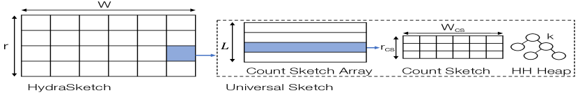
Figure 9. Hydra-sketch structure and configuration parameters.

We now focus on techniques to tune Hydra-sketch’s parameters. As illustrated in Figure 9, Hydra-sketch has six configuration parameters: two parameters ($\mathit{r}$ and $\mathit{w}$) define the structure of the sketch arrays and additional four ($\mathit{L},\ \mathit{w}_{\mathit{CS}},\ \mathit{r}_{\mathit{CS}},$ and $\mathit{k}$) determine the inner structure of the Universal Sketches. The choice of configuration parameters of Hydra-sketch affects its empirical accuracy and memory footprint. For instance, larger $\mathit{w}$ and $\mathit{r}$ values ensure better estimation accuracy but require more memory.

It is often useful to reason about the relative error of the estimation; rephrasing Theorem 2, we can write:

$$\Pr\bigg{[}{-\epsilon_{\mathit{US}}\leq\frac{\widehat{\mathit{G}_{i}}-\mathit{G}_{i}}{\mathit{G}_{i}}\leq\epsilon_{\mathit{US}}+\epsilon\cdot\frac{\mathit{G}_{\mathbb{S}}}{\mathit{G}_{i}}}\bigg{]}\geq 1-\delta.$$

and thus

$$\Pr\left[\frac{\left|\widehat{\mathit{G}_{i}}-\mathit{G}_{i}\right|}{\mathit{G}_{i}}\leq\epsilon_{\mathit{US}}+\epsilon\cdot\frac{\mathit{G}_{\mathbb{S}}}{\mathit{G}_{i}}\right]\geq 1-\delta.$$

That is, we have that with probability $1-\delta$, the relative error is at most $\epsilon_{\mathit{US}}+\epsilon\cdot\frac{\mathit{G}_{\mathbb{S}}}{\mathit{G}_{i}}$. Since $\epsilon_{\mathit{US}},\ \epsilon$, and $\mathit{G}_{\mathbb{S}}$ are determined by the configuration and not a specific subpopulation, we get that the relative error bound is looser if $G_{i}$ is small. Intuitively, if a subpopulation is very small, the noise we get from the colliding subpopulations may be larger than its own statistics.

With that in mind, we consider a quantity $G_{\min}$ that denotes the minimal G-sum for which we want to guarantee some relative error, e.g., of 20%, with a high probability, e.g., 90%. This means that for any subpopulation with a higher G-sum, the error is upper bounded by $\epsilon_{\mathit{US}}+\epsilon\cdot\frac{\mathit{G}_{\mathbb{S}}}{G_{\min}}$. This allows us to derive configuration heuristics for Hydra-sketch as follows:

Controlling the probability of error bounds holding:  From Theorem 2, for the error bound of our example to hold with 90% probability, $1-\delta=0.9$ and, hence, $\delta=0.1$. This translates to $\mathit{r}\approx 3$. Similarly, from Theorem 1, a universal sketch will estimate any $\mathit{G}$-sum function within an $\epsilon_{\mathit{US}}$ factor with probability $1-\delta_{\mathit{US}}$. For probability $90\%$, $\delta_{\mathit{US}}=0.1$ and, thus, $\mathit{r}_{\mathit{CS}}\approx 3$.

Minimizing upper error bound:  To minimize the upper error bound of Hydra-sketch, we need to minimize $E=\epsilon_{\mathit{US}}+\epsilon\frac{\mathit{G}_{\mathbb{S}}}{\mathit{G}_{min}}$ under a memory constraint, $\mathcal{O}(M)=\mathit{w}\times\mathit{w}_{\mathit{US}}$. From Theorems 1 and 2, we know that $\epsilon\approx 1/\mathit{w}$ and $\epsilon_{\mathit{US}}\approx 1/\sqrt{\mathit{w}_{\mathit{US}}}$. This allows us to minimize $E$ for $\mathit{w}$ and $\mathit{w}_{\mathit{US}}$ as follows:

• Solving for $\epsilon_{\mathit{US}}$:  Given the memory constraint, we can write $E=\epsilon_{\mathit{US}}+\frac{\mathit{G}_{\mathbb{S}}}{M\mathit{G}_{min}\epsilon_{\mathit{US}}^{2}}$. Minimizing $E$ over $\epsilon_{\mathit{US}}$ gives us:

  (3) $$\epsilon_{\mathit{US}}=\sqrt[3]{\frac{2\mathit{G}_{\mathbb{S}}}{M\mathit{G}_{min}}}\Rightarrow\mathit{w}_{\mathit{US}}=\Theta(\frac{M\mathit{G}_{min}}{\mathit{G}_{\mathbb{S}}})^{2/3}.$$

• Solving for $\epsilon$:  Similarly, we can write $E=\sqrt{\frac{1}{M\epsilon}}+\epsilon\frac{\mathit{G}_{\mathbb{S}}}{\mathit{G}_{min}}$. Minimizing over $\epsilon$ gives:

  (4) $$\epsilon=\left(\frac{2\sqrt{M}\mathit{G}_{\mathbb{S}}}{\mathit{G}_{min}}\right)^{-2/3}\Rightarrow\mathit{w}=\Theta\left(\frac{\sqrt{M}\mathit{G}_{\mathbb{S}}}{\mathit{G}_{min}}\right)^{2/3}$$

Controlling remaining universal sketch parameters:  Last, we configure the levels ($\mathit{L}$) maintained in each universal sketch instance and the number of heavy keys ($\mathit{k}$) needed to store at each level’s heavy hitter heap. From Theorem 1, $\mathit{L}=\mathcal{O}(\log{\mathit{n}_{\mathit{US}}})$, where $\mathit{n}_{\mathit{US}}$ is the average number of distinct subpopulations summarized at a universal sketch. For the value of $\mathit{k}$, we empirically set its lower bound to $\mathit{k}=\Omega(1/\epsilon_{\mathit{US}}^{2})$. For $\epsilon_{\mathit{US}}=0.1$, this translates to $k\approx 100$.

Let us now see how we can use these guidelines in practice. As an example, let us assume we want the relative error of estimation to not exceed $0.2$ with 90% probability for subpopulations where $\mathit{G}_{i}/\mathit{G}_{\mathbb{S}}\geq 10^{-3}$. Thus, $\mathit{G}_{min}=10^{-3}\cdot\mathit{G}_{\mathbb{S}}$. Let us also assume that $\epsilon_{\mathit{US}}=\epsilon\cdot\frac{\mathit{G}_{\mathbb{S}}}{\mathit{G}_{min}}=0.1$. From Eq. (3), we can get an estimate of memory needed, $M\approx 10^{6}$ needed. Note that here $M$ measures “units of $\mathit{w}_{\mathit{US}}$” i.e., counters. Thus, $\epsilon_{\mathit{US}}=0.1$ and $\mathit{w}_{\mathit{US}}=\Theta(10^{2})$. From $\mathcal{O}(M)=\mathit{w}\cdot\mathit{w}_{\mathit{US}}$, we can further see that also $\mathit{w}=\Theta(10^{2})$.

In §6, we show that these strategies can achieve near optimal tradeoffs. We acknowledge that implementing this workflow assumes that the operator has some prior knowledge about the workload i.e., a rough estimate of the number of subpopulations. We believe this is not an unreasonable requirement in many practical settings.

5. Implementation

This section discusses our implementation of Hydra and the practical performance challenges we faced. Our prototype of Hydra-sketch can be found in (rep, 2022).

Baseline Implementation and Workflow:  We implement Hydra’s workflow (§3) on top of Apache Spark (Zaharia et al., 2016) as Spark’s extensibility allowed us to easily prototype design alternatives. However, Hydra’s workflow can easily fit into different analytics frameworks e.g., Druid (Yang et al., 2014).

Data ingestion happens at the worker nodes. Each worker node splits its input into $\sim$64MB partitions, allocates one Hydra-sketch instance per partition and updates it with that partition’s data. We implement these and Hydra-sketch instances as Spark RDDs. To allocate appropriately configured Hydra-sketch instances, workers rely on configuration manifests distributed by the frontend node.

As a result of splitting input data into smaller batches, each worker node maintains multiple instances of Hydra-sketch. The design of Hydra enables sketch merging due to the well-known linearity property of frequency-based sketches. Therefore, during data ingestion, worker nodes merge Hydra-sketch instances of fully ingested partitions until Hydra is left with one Hydra-sketch instance to query. For sketch merging, we use Spark’s “treeAggregation” module (tre, 2014), thus mitigating the risk of performance bottlenecks.

Query estimation involves both the frontend and the worker nodes. The operator inputs the desired queries and the frontend then generates a query plan for the worker nodes to execute. Estimation results are collected at the frontend node.

An accuracy-improving heuristic:  Recall from §4.4 that after $\mathit{Q}_{i}$ is mapped to a universal sketch, that sketch only stores the frequencies of metric values $\mathit{m}_{j}$. This design, however, does not keep track of which subpopulation $\mathit{Q}_{i}$ each $\mathit{m}_{j}$ maps to. As a result, a universal sketch will return the same estimations for all subpopulations whose data it stores. Our heuristic is simple: Instead of updating each universal sketch with $\mathit{m}_{j}$, we can use a more fine-grained key, i.e., the concatenation of the metric value and its corresponding subpopulation. This way, heavy hitter heaps will maintain heavy counts for each ($\mathit{Q}_{i},\ \mathit{m}_{j}$) pair and will be able to differentiate between them.

Implementation optimizations:  To further reduce the system’s runtime, we introduce a few optimizations:

1. One Large Hash per ($\mathit{Q}_{i}$, $\mathit{m}_{j}$) Pair: Updating Hydra-sketch ($\mathit{Q}_{i}$, $\mathit{m}_{j}$) requires $\mathcal{O}(\mathit{r}\times\mathit{L})$ hash computations, $\mathit{r}$ to identify the universal sketches to update and up to $\mathit{L}$ per universal sketch. We reduce the number of hashes to $\mathcal{O}(1)$ by computing one large 128-bit hash and breaking it down into substrings of variable lengths and treating each substring as a separate hash. Prior analysis (Flajolet and Martin, 1985; Kirsch and Mitzenmacher, 2006) shows that different substrings from the same long hash provide sufficient independence.

2. One Layer Update: In prior universal sketching implementations, the algorithm keeps a heap to track frequent keys per layer. For each datapoint update, the universal sketching needs to update two of its layers on average. In Hydra-sketch, we follow (Yang et al., 2020) and update only the lowest sampled layer per datapoint. This technique reduces the layers updated to one per datapoint, while providing an equivalent implementation.

3. Heap-only sketch merge Merging two Hydra-sketch instances involves iterating over two 2D universal sketches arrays $\text{HS}^{1}$ and $\text{HS}^{2}$ and merging each pair $(\text{HS}^{1}_{k,l},\ \text{HS}^{2}_{k,l})$. This means iterating over the universal sketch layers, summing up corresponding counters, recomputing the heavy elements and re-populating the heavy hitter heaps. However, we find that we can only merge the heavy hitter heaps instead of all counters.

6. Evaluation

We now evaluate Hydra using real-world and synthetic datasets. We provide a sensitivity analysis of our design, and evaluate our configuration strategies and optimizations. In summary:

• Hydra offers $\leq 10$sec query latencies and is $7$-$20\times$ smaller than existing analytics engines.

• Hydra offers $\leq$5% mean errors (combined across statistics) with 90% probability for a broad set of summary statistics at 1/10 of the $ cost of exact analytics engines.

• Thanks to Hydra’s sub-linear (to the number of subpopulations) memory scaling, Hydra achieves close to an order of magnitude improvement in operational cost compared to the best exact analytics baseline.

• Hydra’s sketch configuration strategies ensure near-optimal memory-accuracy tradeoffs.

• Hydra’s performance optimizations improve end-to-end system runtime by 45% compared to a deployment that uses the basic Hydra-sketch design.

6.1. Experimental Methodology

Setup:  We evaluate Hydra on a 20-node cluster of m5.xlarge (4CPU - 16GB memory) AWS servers (pri, 2022). In practice, we observe that nodes have $\approx$10-11GB of available main memory. We allocate 3 CPUs for Hydra and its input data is CSV files that are streamed from AWS S3. We configure Hydra-sketch using the heuristics of §4.6 to ensure a conservative lower error bound of -10% (i.e., $\epsilon_{\mathit{US}}=0.1$) and upper bound of 20% with 90% probability for $\mathit{G}_{min}/\mathit{G}_{\mathbb{S}}=2\cdot 10^{-3}$. We also use the performance optimizations of §5. While these bounds are conservative, they ensure a memory footprint of $<100$MB per Hydra-sketch instance; our results show that the actual errors were much smaller.

Datasets:  We use two real-world datasets and a synthetic trace. Each dataset maps to a different usecase. First, we use CAIDA flow traces (cai, 2021) collected at a backbone link of a Tier1 US-based ISP. The total trace is up to 130GB in initial size and flow data can be clustered in up to approximately 5.6M subpopulations $\mathit{Q}_{i}$. Given that we analyze $\mathit{m}_{j}$ metric values per subpopulation, this dataset contains up to 506M distinct $\langle\mathit{Q}_{i},\mathit{m}_{j}\rangle$ pairs. Second, we use a real-world trace of video session summaries corresponding to one major US-based streaming-video provider. The size of the video-QoE trace is approximate 5GB, with data that we cluster in up to 700k subpopulations and up to 25M $\langle\mathit{Q}_{i},\mathit{m}_{j}\rangle$ pairs. Third, we generate synthetic traces following Zipf distribution with varying skewness (e.g., 0.7 to 0.99).

Summary statistics:  We evaluate Hydra’s accuracy using L1/L2 norms, entropy and cardinality i.e., statistics that map to the queries described in §2. For each subpopulation, we compute the precise value of each statistic as ground truth and then estimate the relative error with respect to Hydra’s accuracy.

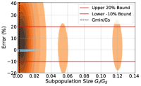
(a) L2-Norm.

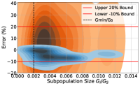
(b) Entropy.

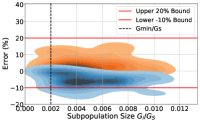
(c) L1-Norm.

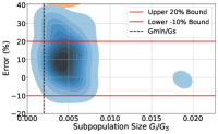
(d) Cardinality.

Figure 10. Error distribution for different data subpopulations for Hydra (blue) and uniform sampling (orange). Red lines indicate the error threshold.

Evaluation baselines:  For our experiments, we compare Hydra against several baselines: From the space of precise analytics we compare with: (1) Spark-SQL: This is a traditional SQL implementation where incoming data record is stored as a row in one (logical) data table. At estimation time, we create a Key-Value store, where the keys are distinct subpopulations $\mathit{Q}_{\mathit{i}}$ and the values are lists of metric values $\mathit{m}_{j}$ per subpopulation; (2) Spark-KV: Here, we summarize incoming data at ingestion time and maintain a Key-Value store where the keys are distinct $\langle\mathit{Q}_{i},\ \mathit{m}_{j}\rangle$ pairs and the values are their respective frequency counts; (3) Druid: This is similar to Spark-KV but uses Druid’s data roll-up feature to generate the key-value store.

From the space of approximate analytics engines, we compare against: (1) Uniform Sampling: We implement 10% uniform sampling at ingestion time and then apply the Spark-KV approach to the sub-sampled data that contains $\approx 82$M distinct $\langle\mathit{Q}_{i},\mathit{m}_{j}\rangle$ pairs; (2) VerdictDB (Park et al., 2018): We deploy VerdictDB on Amazon Redshift and use the default nodes of that service (20 dc2.large nodes, each with 2CPU, 15GB memory and 160GB NVMe-SSD as storage) as backend SQL engine. VerdictDB builds offline samples, so we create hash-based sample tables for cardinality metric and uniform sample tables for L1 and L2 norm. We set sampling rate = 1% for both sample tables. VerdictDB does allow entropy estimations; (3) One Universal Sketch per subpopulation.

6.2. End-to-End Evaluation of Hydra

To evaluate Hydra end-to-end we investigate whether the system meets operators’ requirements as outlined in §2. To that end, we investigate three questions:

What is Hydra’s operating cost compared to our baselines?  We measure the normalized query estimation $ cost for 4 statistics for the CAIDA dataset (130GB, 5.6M subpopulations, 506 distinct $\langle\mathit{Q}_{i},\mathit{m}_{j}\rangle$ pairs). We estimate their normalized cost as VerdictDB on Amazon Redshift constrained us to specific servers with a different pricing model.

Figure 1 depicts Hydra’s cost-accuracy tradeoff. Hydra’s cost is $\sim$2 orders of magnitude smaller than that of Spark-SQL. That is because Spark-SQL processes the entire dataset at query time and because estimation happens at the frontend node. Hydra’s estimation cost is also an order of magnitude lower than Druid’s which uses data summaries created at ingestion. However, as we will see later, Druid’s ingestion is very inefficient. The best performing, precisely accurate baseline is Spark-KV that produces frequency counts for the resulting 506 KV-pairs at ingestion time and uses that for estimating statistics. Spark-KV is $\sim$7$\times$ more expensive than Hydra.

Regarding approximate analytics baselines, we observe that VerdictDB, while very accurate ($\sim$98% mean accuracy for 1% sampling, exhibits large estimation times, comparable to worst-case estimation times in the original VerdictDB paper (Park et al., 2018). When normalized by server cost, VerdictBD’s cost is comparable to Spark-SQL. Hydra’s operational cost is on par with a sampling approach that uniformly samples 10% of all data but whose error can be very large. Perhaps surprisingly, the 10% baseline exhibits higher cost. This is because this baseline still needs to process $\approx 82$M KV pairs and still requires more memory than Hydra. In the case of the smaller video-QoE dataset (not shown due to lack of space), Hydra is only 3$\times$ cheaper than Spark-SQL and approximately as costly as Spark-KV. This smaller gap is due to the smaller size of the dataset. In §6.3, we look at the empirical runtime and memory requirements that explain the observed cost results.

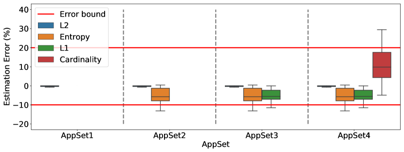
Figure 11. Hydra’s estimation error for the CAIDA dataset.

Does Hydra enable interactive query latencies?  Figure 12 illustrates Hydra’s runtime as a function of the dataset size and the number of data subpopulations for the CAIDA dataset. We can see that Hydra’s query time is $\sim$11sec for 5.6 million data subpopulations, almost one order of magnitude ($7\times$) smaller than that of Spark-KV. We find this to be an acceptable query latency for a framework that is configured to periodically run estimations on streaming data (e.g., every minute) and large volumes of subpopulations. Due to the centralized statistics estimation of Spark-SQL, execution would fail for dataset sizes larger than 30GB. However, even for small input, the querying latency of Spark-SQL is $\sim$2 orders of magnitude larger than Hydra’s. Druid’s ingestion would prematurely terminate for dataset sizes $\geq$60GB because the framework (a) indexes data upon ingestion and (b) is optimized for reads over writes (dru, 2019). We did not focus on improving Druid’s ingestion.

Is Hydra accurate and general across summary statistics?  To evaluate Hydra’s accuracy and generality, we look at the accuracy of four different sets containing different numbers of summary statistics. Figure 11 depicts the boxplot of empirical estimation error for each statistic. Positive error values indicate overestimation errors and negative error values indicate underestimation. For all application sets, Hydra operates under the same resource budget and configuration as described previously. We find that estimating multiple summary statistics does not incur accuracy reduction, compared to when individual statistics are estimated. This highlights Hydra’s generality, which is enabled by the fact that information maintained in the universal sketches is statistic-agnostic and is equally used for multiple statistics of interest. Hydra’s median estimation error is almost 0 for the L2-norm, -5.7% and -5.5% for entropy and L1 norm respectively and 9.8% for cardinality estimation. We can observe that the estimated errors are well within the accuracy threshold that we set. However, for cardinality, we observe a higher median and variance in error values. This is due to a large concentration of $\mathit{G}_{i}$’s near $\mathit{G}_{min}$. Recall from the discussion of §4.6 that Hydra’s error is loosest when $\mathit{G}_{i}\approx\mathit{G}_{min}$ and this allows for higher error variance.

Figure 10 corroborates this observation by depicting the distribution of estimation error values for all summary statistics as a function of the subpopulation’s normalized $\mathit{G}$-sum i.e., $\mathit{G}_{i}/\mathit{G}_{\mathbb{S}}$. Note that for values of $\mathit{G}_{i}/\mathit{G}_{\mathbb{S}}\approx\mathit{G}_{min}/\mathit{G}_{\mathbb{S}}$ the variance of empirical error becomes larger as that is the region where the error is allowed to approach our worst-case error bound. Cardinality estimation using one universal sketch per subpopulation yields estimations with $<7\%$ error. The figure also compares Hydra with uniform sampling and highlights the high variance in error that sampling exhibits. We observe the same behavior for the video-QoE dataset with a mean error across statistics of $\sim$6%.

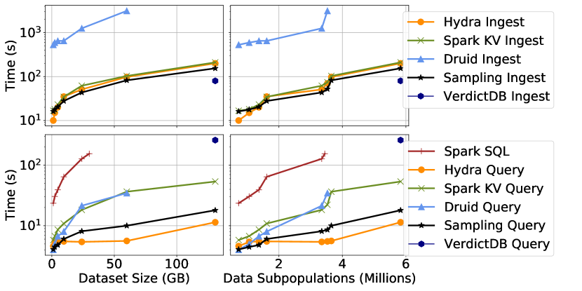
Figure 12. Runtime for CAIDA Dataset

6.3. Detailed Analysis of Hydra-sketch

First, we compare Hydra-sketch’s memory footprint to that of our baselines. Second, we show that our configuration strategies converge to a near-optimal configuration with respect to memory and runtime. Lastly, we show that our performance optimizations reduce Hydra’s runtime by 45%.

Memory Footprint vs. Subpopulations:  Figure 13 shows memory footprint as a function of the number of subpopulations monitored for the CAIDA dataset. Hydra follows the theoretically-expected sub-linear memory scaling as the dataset size and subpopulations increase. Indeed, while we observe that for smaller datasets, a Spark-KV implementation might be preferable in terms of memory footprint (as the size of the sketch instances might even exceed that of the input), this trend is very quickly reversed. This is an observation that is also confirmed for the video-QoE dataset.

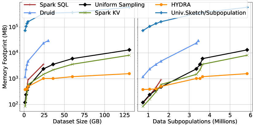
Figure 13. Memory footprint per dataset size and subpopulation. VerdictDB numbers do not expose memory utilizations.

Configuration Heuristics:  Figure 14 depicts the relationship between the memory footprint of Hydra-sketch and its estimation error for different configurations. The estimation error of the figure is that of the L1-Norm of the CAIDA dataset. The optimal configurations simultaneously minimize the estimation error and Hydra-sketch memory footprint (marked with red stars). The orange diamond configuration is the suggested configuration based on the configuration strategies discussed in §4. Thus, our strategies result in a configuration comparable to the optimal configurations. This observation holds across all summary statistics and datasets.

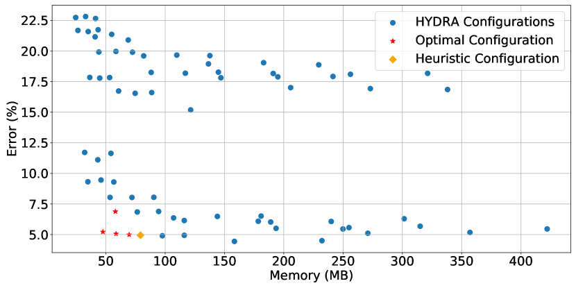
Figure 14. Hydra’s configuration strategies are close to optimal

Analysis of Performance Optimizations:  Figure 15 depicts the cumulative improvement in Hydra’s performance using the performance optimizations of §5. Each datapoint corresponds to a different Hydra-sketch configuration (the Pareto frontier of Figure 14) and we run each configuration twice, once for the basic Hydra-sketch design and once with the performance optimizations. The performance optimizations further reduce the memory footprint of Hydra-sketch and the total system runtime. Table 2 captures Hydra’s runtime reduction after each performance optimization. The baseline is Hydra without optimizations; overall, we see a total performance improvement of 45%.

Table 2. Runtime improvements with performance optimizations

Baseline	Heap-only Merge	One Hash	One Layer Update
100%	92%	64%	55%

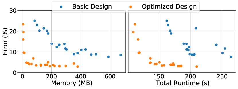
Figure 15. Comparison of the Pareto frontiers of basic and the optimized Hydra-sketch implementation for the same configurations.

Skewness of Dataset:  Figure 16 highlights the difference in estimation accuracy for two synthetic datasets generated with a zipfian distribution. The subpopulations are samples from a zipfian distribution with parameters $\alpha=0.7$ and $\alpha=0.99$ respectively (a value of $\alpha=0$ indicates a perfectly uniform distribution). Our experiment confirms our intuition that the more skewed dataset ensures a better (memory, error) tradeoff. In practice, many real-world datasets are skewed and thus can benefit from being analyzed by Hydra.

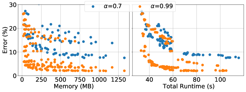
Figure 16. Impact of data skewness on Hydra’s memory footprint and runtime. We use a synthetic dataset where subpopulation sizes are sampled from a Zipfian distribution with parameter $\alpha$.

7. Related work

MapReduce-based Analytics Frameworks:  There are various analytics frameworks that are based on the MapReduce paradigm (Shvachko et al., 2010; Ghemawat et al., 2003). Dryad (Isard et al., 2007) introduced the concept of user-defined functions in general DAG-based workflows. Apache Drill and Impala (Kornacker et al., 2015) are limited to SQL variants. Apache Spark (Zaharia et al., 2016) leverages a DAG-based execution engine and treats unbounded computation as micro-batches. Apache Flink (Carbone et al., 2015) enables pipelined streaming execution for batched and streaming data, offers exactly-one semantics and supports out-of-order processing. Hydra could be built on top of Apache Flink.

Stream Processing Frameworks:  This line of research focuses on the architecture of stream processing systems, answering questions about out-of-order data management, fault tolerance, high-availability, load management, elasticity etc. (Abadi et al., 2005; Arasu et al., 2016; Akidau et al., 2013; kaf, 2017; Balazinska et al., 2005; Carbone et al., 2015; Hwang et al., 2005; Murray et al., 2013; Kazemitabar et al., 2010; ibm, 2022). Fragkoulis et al. analyze the state of the art of stream processing engines (Fragkoulis et al., 2020).

High-dimensional Data Cubes:  Data cubes have been an integral part of online analytics frameworks and enable pre-computing and storing statistics for multidimensional aggregates so that queries can be answered on the fly. However, data cubes suffer from the same scalability challenges as Hydra. Prior works have focused on mechanisms to identify the most frequently queried subsets of the data cube and optimize operations that are performed only on a small subset of dimensions at a time (Li et al., 2004; Gray et al., 1997; Han et al., 2001; Harinarayan et al., 1996; Lakshmanan et al., 2002).

Data Aggregations:  The aggregation-based queries that we discussed in §2 appear in multiple streaming data systems (Bailis et al., 2017; Braun et al., 2015; Cranor et al., 2003; Rabkin et al., 2014; Yang et al., 2014; Agarwal et al., 2013b; Hall et al., 2016) that motivate Hydra. Many of the above frameworks enable approximate analytics but do not fully satisfy operators’ requirements as outlined in §2.

Sampling-based Approaches:  Multiple analytics frameworks use sampling to provide approximate estimations (Acharya et al., 1999; Olston et al., 2009; Chandola et al., 2009; Wang et al., 2015). BlinkDB (Agarwal et al., 2013b) builds stratified samples on its input to reduce query execution time given specific storage budgets. STRAT (Chaudhuri et al., 2007) also uses stratified sampling but instead builds a single sample. SciBORQ (Sidirourgos et al., 2011) builds biased samples based on past query results but cannot provide accuracy guarantees.

Online Aggregation:  Online Aggregation frameworks (Hellerstein et al., 1997; Pansare et al., 2011; Li et al., 2016) continuously refine approximate answers at runtime. In these frameworks, it is up to the user to determine when the acceptable level of accuracy is reached and to terminate estimation. Naturally, this approach is unsuitable for multidimensional telemetry that needs to estimate multiple statistics across data subpopulations.

Data Summaries:  Data “synopses” (e.g., wavelets, histograms, sketches, etc.) have been extensively used for data analytics (Agarwal et al., 2013a; Buragohain and Suri, 2009; Cormode and Muthukrishnan, 2005; Greenwald and Khanna, 2001; Vitter and Wang, 1999; Liu et al., 2016; Wei et al., 2015; Jestes et al., 2011). These data summaries can either be lossless or lossy and they aim to provide efficiency for multidimensional analytics. However, these approaches are tailored to a narrow set of estimation tasks. Gan et al. develop a compact and efficiently mergeable quantile sketch for multidimensional data (Gan et al., 2018).

Several prior efforts explore nested sketches as a solution to the multidimensional distinct counting problem (Xiao et al., 2015; Considine et al., 2009; Ting, 2019, 2018). The CountMin Flajolet-Martin (CM-FM) replaces each integer counter of count-min sketch with a distinct counting sketch (Considine et al., 2009). The CM-FM, while making a step in the right direction for multidimensional analytics, is limited both in terms of the generality and accuracy guarantees it offers (Ting, 2018). Prior work by Ting et al. also targets on cardinality estimation in multidimensional data (Ting, 2019, 2018) but focuses on improving the sketch error bounds. Similar to Hydra, they observe that in distinct counting sketches, accuracy guarantees depend on the characteristics of the underlying data. Their key observation is that the distribution of errors in each counter can be empirically estimated from the sketch itself. By first estimating this distribution, count estimation becomes a statistical estimation and inference problem with a known error distribution. However, computing such error distributions, is computationally heavy in streaming settings as it involves computing maximum likelihood estimators.

8. Discussion and Future Work

Hydra ensures coverage across subpopulations and accuracy guarantees with good resource utilization for subpopulations whose $\mathit{G}_{i}>=\mathit{G}_{min}$. It is up to the operator to determine $\mathit{G}_{min}$. We believe that this is more versatile than pre-selecting specific subpopulations for which accuracy guarantees should apply. Given a $\mathit{G}_{min}$ threshold, Hydra self-selects the subset of important subpopulations.

Hydra opens up avenues for future work. For example, an open question is how to enable dynamic sketch reconfiguration given changing workloads or operator goals. Also, a more system-oriented avenue would involve investigating the applicability of Hydra in the context of in-band network telemetry as part of programmable network elements (Namkung et al., ).

9. Conclusions

Today’s large-scale services require interactive estimates of different statistics across subpopulations of their multidimensional datasets. However, the combinatorial explosion of subpopulations complicates offering multidimensional analytics at a reasonable cost to the operator. We propose Hydra, a sketch-based framework that leverages Hydra-sketch to summarize data streams in sub-linear memory to the number of subpopulations. We show that Hydra is an order of magnitude more efficient than existing analytics engines while ensuring interactive estimation times.

- (1)
- tre (2014) 2014. Spark treeAggregate and treeReduce. https://github.com/apache/spark/pull/1110. (2014). [Online; accessed 16-July-2022].
- lin (2015) 2015. Kafka tops 1 trillion messages per day at linkedin. https://www.datanami.com/2015/09/02/kafka-tops-1-trillion-messages-per-day-at-linkedin/. (2015). [Online; accessed 16-July-2022].
- sur (2015) 2015. SURUS - Anomaly detection at Netflix. https://netflixtechblog.com/rad-outlier-detection-on-big-data-d6b0494371cc. (2015). [Online; accessed 16-July-2022].
- ola (2016) 2016. Approximate Algorithms in Apache spark: Hyperloglog and Quantiles. https://databricks.com/blog/2016/05/19/approximate-algorithms-in-apache-spark-hyperloglog-and-quantiles.html. (2016). [Online; accessed 16-July-2022].
- kaf (2017) 2017. Kafka Streams. https://kafka.apache.org/documentation/streams/. (2017). [Online; accessed 16-July-2022].
- aws (2018) 2018. EC2 DNS Resolution Issues in the Asia Pacific Region. https://aws.amazon.com/message/74876/. (2018). [Online; accessed 16-July-2022].
- cai (2019) 2019. CAIDA Trace. https://www.caida.org/catalog/datasets/monitors/passive-equinix-nyc/. (2019). [Online; accessed 16-July-2022].
- dru (2019) 2019. Druid Ingestion Performance. https://stackoverflow.com/questions/54578482/druid-parquet-poor-ingestion-performance#54580535. (2019). [Online; accessed 16-July-2022].
- aws (2019) 2019. EBS Service Event in the Tokyo Region. https://aws.amazon.com/message/56489/. (2019). [Online; accessed 16-July-2022].
- cai (2021) 2021. CAIDA Network Flow Traces. https://www.caida.org/catalog/datasets/overview/. (2021). [Online; accessed 16-July-2022].
- pri (2022) 2022. Amazon AWS EC2 pricing . https://aws.amazon.com/ec2/pricing/on-demand/. (2022). [Online; accessed 16-July-2022].
- con (2022) 2022. Conviva - Real-time Streaming Video Intelligence. https://www.conviva.com/. (2022). [Online; accessed 16-July-2022].
- rep (2022) 2022. HYDRA repository. https://github.com/antonis-m/HYDRA_VLDB. (2022). [Online; accessed 16-July-2022].
- ibm (2022) 2022. IBM Streams. https://www.ibm.com/cloud/streaming-analytics. (2022). [Online; accessed 16-July-2022].
- Abadi et al. (2005) Daniel J Abadi, Yanif Ahmad, Magdalena Balazinska, Ugur Cetintemel, Mitch Cherniack, Jeong-Hyon Hwang, Wolfgang Lindner, Anurag Maskey, Alex Rasin, Esther Ryvkina, et al. 2005. The design of the borealis stream processing engine.. In Cidr, Vol. 5. 277–289.
- Abraham et al. (2013) Lior Abraham, John Allen, Oleksandr Barykin, Vinayak Borkar, Bhuwan Chopra, Ciprian Gerea, Daniel Merl, Josh Metzler, David Reiss, Subbu Subramanian, et al. 2013. Scuba: Diving into data at facebook. Proceedings of the VLDB Endowment 6, 11 (2013), 1057–1067.
- Acharya et al. (2000) Swarup Acharya, Phillip B Gibbons, and Viswanath Poosala. 2000. Congressional samples for approximate answering of group-by queries. In Proceedings of the 2000 ACM SIGMOD international conference on Management of data. 487–498.
- Acharya et al. (1999) Swarup Acharya, Phillip B Gibbons, Viswanath Poosala, and Sridhar Ramaswamy. 1999. The aqua approximate query answering system. In Proceedings of the 1999 ACM SIGMOD international conference on Management of data. 574–576.
- Agarwal et al. (2013a) Pankaj K Agarwal, Graham Cormode, Zengfeng Huang, Jeff M Phillips, Zhewei Wei, and Ke Yi. 2013a. Mergeable summaries. ACM Transactions on Database Systems (TODS) 38, 4 (2013), 1–28.
- Agarwal et al. (2013b) Sameer Agarwal, Barzan Mozafari, Aurojit Panda, Henry Milner, Samuel Madden, and Ion Stoica. 2013b. BlinkDB: queries with bounded errors and bounded response times on very large data. In Proceedings of the 8th ACM European Conference on Computer Systems. 29–42.
- Akidau et al. (2013) Tyler Akidau, Alex Balikov, Kaya Bekiroğlu, Slava Chernyak, Josh Haberman, Reuven Lax, Sam McVeety, Daniel Mills, Paul Nordstrom, and Sam Whittle. 2013. Millwheel: Fault-tolerant stream processing at internet scale. Proceedings of the VLDB Endowment 6, 11 (2013), 1033–1044.
- Alon et al. (1996) Noga Alon, Yossi Matias, and Mario Szegedy. 1996. The Space Complexity of Approximating the Frequency Moments. In Proc. of ACM STOC.
- Arasu et al. (2016) Arvind Arasu, Brian Babcock, Shivnath Babu, John Cieslewicz, Mayur Datar, Keith Ito, Rajeev Motwani, Utkarsh Srivastava, and Jennifer Widom. 2016. Stream: The stanford data stream management system. In Data Stream Management. Springer, 317–336.
- Armbrust et al. (2015) Michael Armbrust, Reynold S Xin, Cheng Lian, Yin Huai, Davies Liu, Joseph K Bradley, Xiangrui Meng, Tomer Kaftan, Michael J Franklin, Ali Ghodsi, et al. 2015. Spark sql: Relational data processing in spark. In Proceedings of the 2015 ACM SIGMOD international conference on management of data. 1383–1394.
- Asta (2016) A Asta. 2016. Observability at Twitter: technical overview, part i, 2016. (2016).
- Bailis et al. (2017) Peter Bailis, Edward Gan, Samuel Madden, Deepak Narayanan, Kexin Rong, and Sahaana Suri. 2017. Macrobase: Prioritizing attention in fast data. In Proceedings of the 2017 ACM International Conference on Management of Data. 541–556.
- Balazinska et al. (2005) Magdalena Balazinska, Hari Balakrishnan, Samuel Madden, and Michael Stonebraker. 2005. Fault-tolerance in the Borealis distributed stream processing system. In Proceedings of the 2005 ACM SIGMOD international conference on Management of data. 13–24.
- Basat et al. (2020) Ran Ben Basat, Gil Einziger, Michael Mitzenmacher, and Shay Vargaftik. 2020. Faster and more accurate measurement through additive-error counters. In IEEE INFOCOM 2020-IEEE Conference on Computer Communications. IEEE, 1251–1260.
- Basat et al. (2021) Ran Ben Basat, Gil Einziger, Michael Mitzenmacher, and Shay Vargaftik. 2021. SALSA: self-adjusting lean streaming analytics. In 2021 IEEE 37th International Conference on Data Engineering (ICDE). IEEE, 864–875.
- Ben Basat et al. (2017) Ran Ben Basat, Gil Einziger, Roy Friedman, Marcelo C Luizelli, and Erez Waisbard. 2017. Constant time updates in hierarchical heavy hitters. In Proceedings of the Conference of the ACM Special Interest Group on Data Communication. 127–140.
- Braun et al. (2015) Lucas Braun, Thomas Etter, Georgios Gasparis, Martin Kaufmann, Donald Kossmann, Daniel Widmer, Aharon Avitzur, Anthony Iliopoulos, Eliezer Levy, and Ning Liang. 2015. Analytics in motion: High performance event-processing and real-time analytics in the same database. In Proceedings of the 2015 ACM SIGMOD International Conference on Management of Data. 251–264.
- Braverman and Chestnut (2014) Vladimir Braverman and Stephen R Chestnut. 2014. Universal sketches for the frequency negative moments and other decreasing streaming sums. arXiv preprint arXiv:1408.5096 (2014).
- Braverman and Ostrovsky (2010) Vladimir Braverman and Rafail Ostrovsky. 2010. Zero-one frequency laws. In Proceedings of the forty-second ACM symposium on Theory of computing. 281–290.
- Buragohain and Suri (2009) Chiranjeeb Buragohain and Subhash Suri. 2009. Quantiles on Streams. (2009).
- Carbone et al. (2015) Paris Carbone, Asterios Katsifodimos, Stephan Ewen, Volker Markl, Seif Haridi, and Kostas Tzoumas. 2015. Apache flink: Stream and batch processing in a single engine. Bulletin of the IEEE Computer Society Technical Committee on Data Engineering 36, 4 (2015).
- Chaiken et al. (2008) Ronnie Chaiken, Bob Jenkins, Per-Åke Larson, Bill Ramsey, Darren Shakib, Simon Weaver, and Jingren Zhou. 2008. Scope: easy and efficient parallel processing of massive data sets. Proceedings of the VLDB Endowment 1, 2 (2008), 1265–1276.
- Chandola et al. (2009) Varun Chandola, Arindam Banerjee, and Vipin Kumar. 2009. Anomaly Detection: A Survey. ACM Comput. Surv. 41, 3, Article 15 (July 2009), 58 pages. https://doi.org/10.1145/1541880.1541882
- Chaudhuri et al. (2007) Surajit Chaudhuri, Gautam Das, and Vivek Narasayya. 2007. Optimized stratified sampling for approximate query processing. ACM Transactions on Database Systems (TODS) 32, 2 (2007), 9–es.
- Chaudhuri et al. (2017) Surajit Chaudhuri, Bolin Ding, and Srikanth Kandula. 2017. Approximate query processing: No silver bullet. In Proceedings of the 2017 ACM International Conference on Management of Data. 511–519.
- Chen et al. (2020) Xiaoqi Chen, Shir Landau-Feibish, Mark Braverman, and Jennifer Rexford. 2020. Beaucoup: Answering many network traffic queries, one memory update at a time. In Proceedings of the Annual conference of the ACM Special Interest Group on Data Communication on the applications, technologies, architectures, and protocols for computer communication. 226–239.
- Considine et al. (2009) Jeffrey Considine, Marios Hadjieleftheriou, Feifei Li, John Byers, and George Kollios. 2009. Robust approximate aggregation in sensor data management systems. ACM Transactions on Database Systems (TODS) 34, 1 (2009), 1–35.
- Cormode et al. (2012) Graham Cormode, Minos Garofalakis, Peter J Haas, and Chris Jermaine. 2012. Synopses for massive data: Samples, histograms, wavelets, sketches. Foundations and Trends in Databases 4, 1–3 (2012), 1–294.
- Cormode and Muthukrishnan (2005) Graham Cormode and Shan Muthukrishnan. 2005. An improved data stream summary: the count-min sketch and its applications. Journal of Algorithms 55, 1 (2005), 58–75.
- Cranor et al. (2003) Chuck Cranor, Theodore Johnson, Oliver Spataschek, and Vladislav Shkapenyuk. 2003. Gigascope: A stream database for network applications. In Proceedings of the 2003 ACM SIGMOD international conference on Management of data. 647–651.
- Durand and Flajolet (2003) Marianne Durand and Philippe Flajolet. 2003. Loglog counting of large cardinalities. In European Symposium on Algorithms. Springer, 605–617.
- Feldmann et al. (2001) Anja Feldmann, Albert Greenberg, Carsten Lund, Nick Reingold, Jennifer Rexford, and Fred True. 2001. Deriving traffic demands for operational IP networks: Methodology and experience. IEEE/ACM Transactions On Networking 9, 3 (2001), 265–279.
- Flajolet and Martin (1985) Philippe Flajolet and G Nigel Martin. 1985. Probabilistic counting algorithms for data base applications. Journal of computer and system sciences 31, 2 (1985), 182–209.
- Fragkoulis et al. (2020) Marios Fragkoulis, Paris Carbone, Vasiliki Kalavri, and Asterios Katsifodimos. 2020. A Survey on the Evolution of Stream Processing Systems. arXiv preprint arXiv:2008.00842 (2020).
- Gan et al. (2020) Edward Gan, Peter Bailis, and Moses Charikar. 2020. Coopstore: Optimizing precomputed summaries for aggregation. Proceedings of the VLDB Endowment 13, 12 (2020), 2174–2187.
- Gan et al. (2018) Edward Gan, Jialin Ding, Kai Sheng Tai, Vatsal Sharan, and Peter Bailis. 2018. Moment-based quantile sketches for efficient high cardinality aggregation queries. arXiv preprint arXiv:1803.01969 (2018).
- Ghemawat et al. (2003) Sanjay Ghemawat, Howard Gobioff, and Shun-Tak Leung. 2003. The Google file system. In Proceedings of the nineteenth ACM symposium on Operating systems principles. 29–43.
- Gray et al. (1997) Jim Gray, Surajit Chaudhuri, Adam Bosworth, Andrew Layman, Don Reichart, Murali Venkatrao, Frank Pellow, and Hamid Pirahesh. 1997. Data cube: A relational aggregation operator generalizing group-by, cross-tab, and sub-totals. Data mining and knowledge discovery 1, 1 (1997), 29–53.
- Greenwald and Khanna (2001) Michael Greenwald and Sanjeev Khanna. 2001. Space-efficient online computation of quantile summaries. ACM SIGMOD Record 30, 2 (2001), 58–66.
- Gupta et al. (2018) Arpit Gupta, Rob Harrison, Marco Canini, Nick Feamster, Jennifer Rexford, and Walter Willinger. 2018. Sonata: Query-driven streaming network telemetry. In Proceedings of the 2018 conference of the ACM special interest group on data communication. 357–371.
- Hall et al. (2016) Alex Hall, Alexandru Tudorica, Filip Buruiana, Reimar Hofmann, Silviu-Ionut Ganceanu, and Thomas Hofmann. 2016. Trading off accuracy for speed in PowerDrill. (2016).
- Han et al. (2001) Jiawei Han, Jian Pei, Guozhu Dong, and Ke Wang. 2001. Efficient computation of iceberg cubes with complex measures. In Proceedings of the 2001 ACM SIGMOD international conference on Management of data. 1–12.
- Harinarayan et al. (1996) Venky Harinarayan, Anand Rajaraman, and Jeffrey D Ullman. 1996. Implementing data cubes efficiently. Acm Sigmod Record 25, 2 (1996), 205–216.
- Hellerstein et al. (1997) Joseph M Hellerstein, Peter J Haas, and Helen J Wang. 1997. Online aggregation. In Proceedings of the 1997 ACM SIGMOD international conference on Management of data. 171–182.
- Hill et al. (2017) Daniel N Hill, Houssam Nassif, Yi Liu, Anand Iyer, and SVN Vishwanathan. 2017. An efficient bandit algorithm for realtime multivariate optimization. In Proceedings of the 23rd ACM SIGKDD International Conference on Knowledge Discovery and Data Mining. 1813–1821.
- Hwang et al. (2005) J-H Hwang, Magdalena Balazinska, Alex Rasin, Ugur Cetintemel, Michael Stonebraker, and Stan Zdonik. 2005. High-availability algorithms for distributed stream processing. In 21st International Conference on Data Engineering (ICDE’05). IEEE, 779–790.
- Isard et al. (2007) Michael Isard, Mihai Budiu, Yuan Yu, Andrew Birrell, and Dennis Fetterly. 2007. Dryad: distributed data-parallel programs from sequential building blocks. In Proceedings of the 2nd ACM SIGOPS/EuroSys European Conference on Computer Systems 2007. 59–72.
- Jestes et al. (2011) Jeffrey Jestes, Ke Yi, and Feifei Li. 2011. Building wavelet histograms on large data in mapreduce. arXiv preprint arXiv:1110.6649 (2011).
- Jiang et al. (2016) Junchen Jiang, Vyas Sekar, Henry Milner, Davis Shepherd, Ion Stoica, and Hui Zhang. 2016. CFA: A Practical Prediction System for Video QoE Optimization. In Proceedings of the 13th Usenix Conference on Networked Systems Design and Implementation (NSDI’16). USENIX Association, Berkeley, CA, USA, 137–150. http://dl.acm.org/citation.cfm?id=2930611.2930621
- Jiang et al. (2013) Junchen Jiang, Vyas Sekar, Ion Stoica, and Hui Zhang. 2013. Shedding light on the structure of internet video quality problems in the wild. In Proceedings of the ninth ACM conference on Emerging networking experiments and technologies. ACM, 357–368.
- Johari et al. (2017) Ramesh Johari, Pete Koomen, Leonid Pekelis, and David Walsh. 2017. Peeking at a/b tests: Why it matters, and what to do about it. In Proceedings of the 23rd ACM SIGKDD International Conference on Knowledge Discovery and Data Mining. 1517–1525.
- Kazemitabar et al. (2010) Seyed Jalal Kazemitabar, Ugur Demiryurek, Mohamed Ali, Afsin Akdogan, and Cyrus Shahabi. 2010. Geospatial stream query processing using Microsoft SQL Server StreamInsight. Proceedings of the VLDB Endowment 3, 1-2 (2010), 1537–1540.
- Kirsch and Mitzenmacher (2006) Adam Kirsch and Michael Mitzenmacher. 2006. Less hashing, same performance: building a better bloom filter. In European Symposium on Algorithms. Springer, 456–467.
- Kornacker et al. (2015) Marcel Kornacker, Alexander Behm, Victor Bittorf, Taras Bobrovytsky, Casey Ching, Alan Choi, Justin Erickson, Martin Grund, Daniel Hecht, Matthew Jacobs, et al. 2015. Impala: A Modern, Open-Source SQL Engine for Hadoop.. In Cidr, Vol. 1. 9.
- Lakshmanan et al. (2002) Laks VS Lakshmanan, Jian Pei, and Jiawei Han. 2002. Quotient cube: How to summarize the semantics of a data cube. In VLDB’02: Proceedings of the 28th International Conference on Very Large Databases. Elsevier, 778–789.
- Li et al. (2016) Feifei Li, Bin Wu, Ke Yi, and Zhuoyue Zhao. 2016. Wander join: Online aggregation via random walks. In Proceedings of the 2016 International Conference on Management of Data. 615–629.
- Li et al. (2004) Xiaolei Li, Jiawei Han, and Hector Gonzalez. 2004. High-dimensional OLAP: A minimal cubing approach. In Proceedings of the Thirtieth international conference on Very large data bases-Volume 30. 528–539.
- Liu et al. (2016) Zaoxing Liu, Antonis Manousis, Gregory Vorsanger, Vyas Sekar, and Vladimir Braverman. 2016. One sketch to rule them all: Rethinking network flow monitoring with univmon. In Proceedings of the 2016 ACM SIGCOMM Conference. 101–114.
- Ma and Triantafillou (2019) Qingzhi Ma and Peter Triantafillou. 2019. Dbest: Revisiting approximate query processing engines with machine learning models. In Proceedings of the 2019 International Conference on Management of Data. 1553–1570.
- Melnik et al. (2010) Sergey Melnik, Andrey Gubarev, Jing Jing Long, Geoffrey Romer, Shiva Shivakumar, Matt Tolton, and Theo Vassilakis. 2010. Dremel: interactive analysis of web-scale datasets. Proceedings of the VLDB Endowment 3, 1-2 (2010), 330–339.
- Minton and Price (2014) Gregory T Minton and Eric Price. 2014. Improved concentration bounds for count-sketch. In Proceedings of the twenty-fifth annual ACM-SIAM symposium on Discrete algorithms. SIAM, 669–686.
- Murray et al. (2013) Derek G Murray, Frank McSherry, Rebecca Isaacs, Michael Isard, Paul Barham, and Martín Abadi. 2013. Naiad: a timely dataflow system. In Proceedings of the Twenty-Fourth ACM Symposium on Operating Systems Principles. 439–455.
- (78) Hun Namkung, Zaoxing Liu, Daehyeok Kim, Vyas Sekar, Peter Steenkiste, Guyue Liu, Ao Li, Christopher Canel, Adithya Abraham Philip, Ranysha Ware, et al. Sketchlib: Enabling efficient sketch-based monitoring on programmable switches. NSDI.
- Olston et al. (2009) Christopher Olston, Edward Bortnikov, Khaled Elmeleegy, Flavio Junqueira, and Benjamin Reed. 2009. Interactive Analysis of Web-Scale Data.. In CIDR. Citeseer.
- Olston et al. (2008) Christopher Olston, Benjamin Reed, Utkarsh Srivastava, Ravi Kumar, and Andrew Tomkins. 2008. Pig latin: a not-so-foreign language for data processing. In Proceedings of the 2008 ACM SIGMOD international conference on Management of data. 1099–1110.
- Pansare et al. (2011) Niketan Pansare, Vinayak Borkar, Chris Jermaine, and Tyson Condie. 2011. Online aggregation for large mapreduce jobs. Proceedings of the VLDB Endowment 4, 11 (2011), 1135–1145.
- Park et al. (2018) Yongjoo Park, Barzan Mozafari, Joseph Sorenson, and Junhao Wang. 2018. Verdictdb: Universalizing approximate query processing. In Proceedings of the 2018 International Conference on Management of Data. 1461–1476.
- Pelkonen et al. (2015) Tuomas Pelkonen, Scott Franklin, Justin Teller, Paul Cavallaro, Qi Huang, Justin Meza, and Kaushik Veeraraghavan. 2015. Gorilla: A fast, scalable, in-memory time series database. Proceedings of the VLDB Endowment 8, 12 (2015), 1816–1827.
- Rabkin et al. (2014) Ariel Rabkin, Matvey Arye, Siddhartha Sen, Vivek S Pai, and Michael J Freedman. 2014. Aggregation and degradation in jetstream: Streaming analytics in the wide area. In 11th USENIX Symposium on Networked Systems Design and Implementation (NSDI 14). 275–288.
- Ramachandran et al. (2008) Anirudh Ramachandran, Srinivasan Seetharaman, Nick Feamster, and Vijay Vazirani. 2008. Fast monitoring of traffic subpopulations. In Proceedings of the 8th ACM SIGCOMM conference on Internet measurement. 257–270.
- Shvachko et al. (2010) Konstantin Shvachko, Hairong Kuang, Sanjay Radia, and Robert Chansler. 2010. The hadoop distributed file system. In 2010 IEEE 26th symposium on mass storage systems and technologies (MSST). Ieee, 1–10.
- Sidirourgos et al. (2011) Lefteris Sidirourgos, Martin L Kersten, Peter A Boncz, et al. 2011. Sciborq: scientific data management with bounds on runtime and quality.. In CIDR, Vol. 11. 296–301.
- Thusoo et al. (2009) Ashish Thusoo, Joydeep Sen Sarma, Namit Jain, Zheng Shao, Prasad Chakka, Suresh Anthony, Hao Liu, Pete Wyckoff, and Raghotham Murthy. 2009. Hive: a warehousing solution over a map-reduce framework. Proceedings of the VLDB Endowment 2, 2 (2009), 1626–1629.
- Ting (2018) Daniel Ting. 2018. Count-min: optimal estimation and tight error bounds using empirical error distributions. In Proceedings of the 24th ACM SIGKDD International Conference on Knowledge Discovery & Data Mining. 2319–2328.
- Ting (2019) Daniel Ting. 2019. Approximate distinct counts for billions of datasets. In Proceedings of the 2019 International Conference on Management of Data. 69–86.
- Vartak et al. (2015) Manasi Vartak, Sajjadur Rahman, Samuel Madden, Aditya Parameswaran, and Neoklis Polyzotis. 2015. Seedb: Efficient data-driven visualization recommendations to support visual analytics. In Proceedings of the VLDB Endowment International Conference on Very Large Data Bases, Vol. 8. NIH Public Access, 2182.
- Vitter and Wang (1999) Jeffrey Scott Vitter and Min Wang. 1999. Approximate computation of multidimensional aggregates of sparse data using wavelets. Acm Sigmod Record 28, 2 (1999), 193–204.
- Wang et al. (2015) Lu Wang, Robert Christensen, Feifei Li, and Ke Yi. 2015. Spatial online sampling and aggregation. Proceedings of the VLDB Endowment 9, 3 (2015), 84–95.
- Wei et al. (2015) Zhewei Wei, Ge Luo, Ke Yi, Xiaoyong Du, and Ji-Rong Wen. 2015. Persistent data sketching. In Proceedings of the 2015 ACM SIGMOD international conference on Management of Data. 795–810.
- Xiao et al. (2015) Qingjun Xiao, Shigang Chen, Min Chen, and Yibei Ling. 2015. Hyper-compact virtual estimators for big network data based on register sharing. In Proceedings of the 2015 ACM SIGMETRICS International Conference on Measurement and Modeling of Computer Systems. 417–428.
- Xie et al. (2005) Yinglian Xie, Vyas Sekar, David A Maltz, Michael K Reiter, and Hui Zhang. 2005. Worm origin identification using random moonwalks. In 2005 IEEE Symposium on Security and Privacy (S&P’05). IEEE, 242–256.
- Yang et al. (2014) Fangjin Yang, Eric Tschetter, Xavier Léauté, Nelson Ray, Gian Merlino, and Deep Ganguli. 2014. Druid: A real-time analytical data store. In Proceedings of the 2014 ACM SIGMOD international conference on Management of data. 157–168.
- Yang et al. (2020) Mingran Yang, Junbo Zhang, Akshay Gadre, Zaoxing Liu, Swarun Kumar, and Vyas Sekar. 2020. Joltik: enabling energy-efficient” future-proof” analytics on low-power wide-area networks. In Proceedings of the 26th Annual International Conference on Mobile Computing and Networking. 1–14.
- Yu et al. (2013) Minlan Yu, Lavanya Jose, and Rui Miao. 2013. Software Defined Traffic Measurement with OpenSketch. In 10th USENIX Symposium on Networked Systems Design and Implementation (NSDI 13). 29–42.
- Zaharia et al. (2016) Matei Zaharia, Reynold S Xin, Patrick Wendell, Tathagata Das, Michael Armbrust, Ankur Dave, Xiangrui Meng, Josh Rosen, Shivaram Venkataraman, Michael J Franklin, et al. 2016. Apache spark: a unified engine for big data processing. Commun. ACM 59, 11 (2016), 56–65.