Moving sum procedure for change point detection under piecewise linearity

Abstract

We propose a computationally and statistically efficient procedure for segmenting univariate data under piecewise linearity. The proposed moving sum (MOSUM) methodology detects multiple change points where the underlying signal undergoes discontinuous jumps and/or slope changes. It controls the family-wise error rate at a given significance level and achieves consistency in multiple change point detection, with a minimax optimal estimation rate when the signal is piecewise linear and continuous, all under weak assumptions permitting serial dependence and heavy-tailedness. Computationally, the complexity of the MOSUM procedure is $O(n)$, which, combined with its good performance on simulated datasets, makes it highly attractive compared to the existing methods. We further demonstrate its good performance on a real data example on rolling element-bearing prognostics.

Keywords: Data segmentation; Piecewise linear model; Change point analysis; MOSUM

1 Introduction

Data segmentation, a.k.a. multiple change point detection, is an active field of research in time series analysis and signal processing, and numerous applications are found, e.g., in climatology (Reeves et al.,, 2007), genomics (Niu and Zhang,, 2012), neuroscience (Aston and Kirch,, 2012), neurophysiology (Messer et al.,, 2014) and finance (Bardwell et al.,, 2019). We refer to Truong et al., (2020) and Cho and Kirch, 2022a for an overview of the recent developments. In particular, the review articles demonstrate that the problem of detecting multiple change points in the mean of univariate time series has received significant attention, and several state-of-the-art methods exist for this canonical change point problem.

By contrast, there are far fewer papers that address the problem of detecting change points under piecewise linearity, where the signal underlying the data undergoes discontinuous jumps or slope changes. In practice, it is rarely known in advance whether the data is best approximated by a piecewise constant signal or a piecewise linear one, and many time series datasets exhibit complex features that may not be represented as piecewise constant functions. We demonstrate this using a dataset first analyzed by Qiu et al., (2006). Accelerometers were installed on four test bearings and recorded their vibrations from February 12th to February 19th in 2004, when a failure occurred in one of the bearings. Focusing on the data obtained from the faulty bearing, Figure 1 shows that a drastic change in the trend is observed after February 16th, followed by severe instabilities from February 17th onward. This demonstrates the necessity for a methodology that detects both abrupt jumps and continuous changes in the trend while being agnostic to the type of changes in order to infer the onset of the mechanical fault.

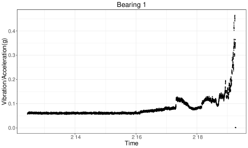
Figure 1: Time series data ($n=9830$) generated by taking a one-minute average of the raw observations recorded by an accelerometer installed on a faulty test bearing between 10:32:39 on February 12th and 06:22:39 on February 19th in 2004. We take the average to remove any periodic vibration and focus on detecting changes in the trend of the data.

There are several methods for detecting the changes under piecewise linearity, which, as in the case of the canonical mean change point problem (Cho and Kirch, 2022a, ), are categorized into those based on the application of localized testing, and those based on global optimization of an objective function. In the first category, Baranowski et al., (2019) proposed the narrowest-over-threshold (NOT) methodology, which, as a variant of the wild binary segmentation (Fryzlewicz,, 2014), identifies local sections of the data that contain features (i.e., slope or intercept changes) using contrast functions tailored for detecting the particular changes of interest. Maeng and Fryzlewicz, (2023) found a sparse representation of the data via wavelets constructed for well-capturing piecewise linear signals, extending the approach of Fryzlewicz, (2018). Anastasiou and Fryzlewicz, (2022) suggested localizing change points by iteratively expanding the local intervals under inspection. Methods based on minimizing $\ell_{0}$-penalized cost functions belong to the second category, which includes the CPOP methodology (Fearnhead et al.,, 2019), where the dynamic programming popularly adopted for the mean change point detection problems (Jackson et al.,, 2005; Killick et al.,, 2012), is also employed to find the best piecewise linear and continuous fit to the data. Yu et al., (2022) provide theoretical investigation into such an estimator for the problem of localizing change points in piecewise polynomials of general degrees. In addition, we mention the literature on piecewise polynomial regression or spline smoothing with the knots at fixed (Green and Silverman,, 1993) or unfixed (Mammen and van de Geer,, 1997; Tibshirani,, 2014; Guntuboyina et al.,, 2020; Spiriti et al.,, 2013) locations where typically, the aim is to control the $\ell_{2}$-risk of the estimated signal. The problem of real-time monitoring of changes in streaming settings has also received attention (Wu et al.,, 2015; Wen et al.,, 2018; Xu et al.,, 2023), but our primary focus lies in offline data segmentation.

We propose a moving window-based methodology for the data segmentation problem under piecewise linearity. Referred to as the moving sum (MOSUM) procedure, it scans for multiple jumps and slope changes using the detector statistic which compares the local estimators of intercept and slope parameters from adjacent moving windows. MOSUM procedures have popularly been adopted in the data segmentation literature for their computational efficiency, from detecting change points in the mean of univariate time series (Eichinger and Kirch,, 2018; Cho and Kirch, 2022b, ) and regime shifts in multivariate renewal processes (Kirch and Klein,, 2023), to segmenting multivariate (Yau and Zhao,, 2016) and high-dimensional (Cho et al.,, 2023) time series under parametric models. Kirch and Reckruehm, (2022) provided a general change point detection methodology based on estimating equations. Distinguished from these efforts, we permit the presence of time-varying trends in the data, which requires careful treatment both theoretically and methodologically.

The proposed MOSUM procedure is shown to (i) control the (asymptotic) family-wise error rate at a given significance level, (ii) achieve consistency in estimating both the total number and the locations of the change points, and further, (iii) exactly match the minimax optimal rate of estimation when the underlying signal is piecewise linear and continuous. Our theoretical results are derived under mild conditions permitting serial dependence and heavy-tailedness, which are considerably more general than the independence and (sub)-Gaussianity assumptions in the existing literature. Computationally, thanks to the use of moving windows, the MOSUM procedure is highly efficient with the $O(n)$ complexity, making it particularly attractive in analyzing large datasets. The R code implementing our method is available at https://github.com/Joonpyo-Kim/MovingSumLin.

2 MOSUM procedure under piecewise linearity

2.1 Methodology

We consider the following model

$$X_{i}=f_{i}+\epsilon_{i}=\sum_{j=1}^{J_{n}+1}(\alpha_{0,j}+\alpha_{1,j}t_{i})\cdot\mathbb{I}_{\{k_{j-1}+1\leq i\leq k_{j}\}}+\epsilon_{i},\quad i=1,\ldots,n,$$ (1)

where $t_{i}=i\Delta t$ denotes the time points with $[0,T]$ as the observation period and $\Delta t=T/n$. We assume that $\{\epsilon_{i}\}_{i=1}^{n}$ is a stationary sequence of random variables with $\mathsf{E}(\epsilon_{i})=0$, $\mathsf{Var}(\epsilon_{i})=\sigma^{2}$ and the long-run variance (LRV) $\tau^{2}=\sigma^{2}+2\sum_{h=1}^{\infty}\mathsf{Cov}(\epsilon_{0},\epsilon_{h})$, where $\sigma^{2},\tau^{2}\in(0,\infty)$, and it is allowed to be serially dependent as specified later. Under the model (1), $f_{i}=\mathsf{E}(X_{i})$ is piecewise linear with $J_{n}$ change points denoted by $k_{j},\,j=1,\ldots,J_{n}$ (with $k_{0}=0$ and $k_{J_{n}+1}=n$), at which either the intercept or the slope or both, undergo changes. That is, denoting by $\boldsymbol{\alpha}_{j}=(\alpha_{0,j},\alpha_{1,j})^{\top}$, we have $\boldsymbol{\alpha}_{j}\neq\boldsymbol{\alpha}_{j+1}$ for all $j=1,\ldots,J_{n}$. We permit $J_{n}\to\infty$ as $n\to\infty$ provided that change points are sufficiently distanced away from one another as specified later. When $\alpha_{1,j}=0$ for all $j$, the model (1) becomes the canonical change point model with piecewise constant $f_{i}$.

Under the model in (1), our aim is two-fold, (i) to test the null hypothesis of no change point $\mathcal{H}_{0}:\,J_{n}=0$ against $\mathcal{H}_{1}:\,J_{n}>0$, and (ii) if $\mathcal{H}_{0}$ is rejected, to estimate the total number $J_{n}$ and the locations $k_{j}$ of the change points. To achieve the above goals, we propose a moving window-based methodology that scans for (possibly) multiple change points by comparing the local parameter estimates from the adjacent windows. Specifically, let $G$ denote a bandwidth satisfying $2G<n$, and define $\mathcal{I}^{+}(k)=\{k+1,\ldots,k+G\}$ and $\mathcal{I}^{-}(k)=\{k-G+1,\ldots,k\}$ for $G\leq k\leq n-G$. Then, at each time point $k$, we regress $X_{i}$ onto $\mathbf{x}_{i,k}=(1,(i-k)/G)^{\top}$ for $i\in\mathcal{I}^{+}(k)$ (resp. $\mathcal{I}^{-}(k)$) to obtain the least squares estimator $\widehat{\boldsymbol{\beta}}^{+}(k)=(\widehat{\beta}_{0}^{+}(k),\widehat{\beta}_{1}^{+}(k))^{\top}$ (resp. $\widehat{\boldsymbol{\beta}}^{-}(k)$). The choice of the regressor $\mathbf{x}_{i,k}$ allows the intercept and the slope estimators to be treated on an equal footing. Then, if neither discontinuous jump nor slope change occurs on $\mathcal{I}^{-}(k)\cup\mathcal{I}^{+}(k)$, we expect $\|\widehat{\boldsymbol{\beta}}^{+}(k)-\widehat{\boldsymbol{\beta}}^{-}(k)\|$ to be small and vice versa, where $\|\cdot\|$ denotes the Euclidean norm.

Based on these observations, we propose the following Wald-type MOSUM statistic

$$W_{k,n}(G)=\frac{\sqrt{G}}{\widehat{\tau}_{k}}\left\|\boldsymbol{\Sigma}^{-1/2}\left(\widehat{\boldsymbol{\beta}}^{+}(k)-\widehat{\boldsymbol{\beta}}^{-}(k)\right)\right\|,\,G\leq k\leq n-G,$$ (2)

where $\boldsymbol{\Sigma}$ is a $2\times 2$ diagonal matrix with diagonal elements 8 and 24 (motivated by the distribution of $\widehat{\boldsymbol{\beta}}^{+}(k)-\widehat{\boldsymbol{\beta}}^{-}(k)$ under $\mathcal{H}_{0}$), and $\widehat{\tau}_{k}>0$ denotes a (possibly) location-dependent estimator of $\tau$. Then, for some $\alpha\in(0,1)$, we reject $\mathcal{H}_{0}$ if $W_{n}(G):=\max_{G\leq k\leq n-G}W_{k,n}(G)$ exceeds a critical value $C_{n}(G,\alpha)$ obtained from the asymptotic null distribution of $W_{n}(G)$ (see Theorem 2.1 below), the choice of which ensures that the test controls the family-wise error rate at the prescribed level $\alpha$ when $W_{k,n}(G)$ is scanned over $k=G,\ldots,n-G$.

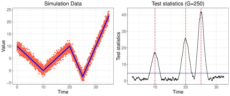
Figure 2: A realization from a dataset of length $n=3500$ generated by the model (M2) and the errors in (E1) (see Section 4) with $\sigma=1$ (left) and the corresponding MOSUM statistics $W_{k,n}(G)$ with $G=250$ for all $k=G,\ldots,n-G$ (right). Estimated change point locations (vertical broken lines) and $C_{n}(G,\alpha)$ with $\alpha=0.05$ (horizontal line) are also displayed.

By construction, the statistic $W_{k,n}(G)$ is expected to take large values in the intervals around the change points $k_{j},\,j=1,\ldots,J_{n}$, while its value is small for $k$ sufficiently far from the change points, see the right panel of Figure 2. Therefore, we propose to estimate their locations with the local maximizers of $W_{k,n}(G)$ around which the statistics are significantly large by exceeding $C_{n}(G,\alpha)$. Specifically, motivated by the selection rule proposed by Eichinger and Kirch, (2018) for the mean change point detection problem, we identify all pairs of indices $(v_{j},w_{j}),\,j=1,\ldots,\widehat{J}_{n}$, which simultaneously satisfy: (a) $W_{k,n}(G)\geq C_{n}(G,\alpha)$ for $k\in\{v_{j},\ldots,w_{j}\}$, (b) $W_{k,n}(G)<C_{n}(G,\alpha)$ for $k\in\{v_{j}-1,w_{j}+1\}$, and (c) $w_{j}-v_{j}\geq\eta G$ with a fixed $\eta\in(0,1/2)$. Then, we estimate $J_{n}$ by $\widehat{J}_{n}$ and the locations of the change points by $\widehat{k}_{j}=\underset{v_{j}\leq k\leq w_{j}}{\arg\max}\,W_{k,n}(G)$ for $j=1,\ldots,\widehat{J}_{n}$. With $\eta$ appropriately chosen, this rule allows for simultaneous estimation of all the $J_{n}$ change points without incurring any duplicate estimators.

Remark 2.1.

The statistic $W_{k,n}(G)$ in (2) bears a resemblance to the Wald-type MOSUM statistic applied to the change point detection problem in linear regression (Kirch and Reckruehm,, 2022), a problem extensively studied in the change point literature (Csörgő and Horváth,, 1997; Bai and Perron,, 1998, 2003). However, such methods have typically been analyzed under the (second-order) stationarity of the covariates, which precludes the existence of the (possibly) time-varying trend. As such, the investigation into the behavior of $W_{k,n}(G)$ requires a careful treatment of the presence of the trend when investigating the theoretical properties, which we discuss in Section 2.2.

2.2 Theoretical properties

2.2.1 Asymptotic null distribution

In this section, we derive the asymptotic null distribution of $W_{n}(G)$ from which the critical value $C_{n}(G,\alpha)$ is obtained. On the stationary sequence $\{\epsilon_{i}\}_{i\in\mathbb{Z}}$, we require mild conditions permitting serial dependence and heavy-tailedness, which greatly relaxes the independence and (sub-)Gaussianity assumptions in the literature on piecewise linear modelling.

1. There exists a standard Wiener process $\{W(t):\,0\leq t<\infty\}$ and $\nu>0$ such that $|\sum_{i=1}^{n}\epsilon_{i}-\tau W(n)|=O(n^{1/(2+\nu)})$ a.s.

2. There exist constants $\gamma>2$ and $C_{0},C_{1}>0$ such that, for any $0\leq\ell<r<\infty$, we have $\mathsf{E}(|\sum_{i=\ell+1}^{r}\epsilon_{i}|^{\gamma})\leq C_{0}|r-\ell|^{\gamma/2}$ and $\mathsf{E}(|\sum_{i=\ell+1}^{r}i\epsilon_{i}|^{\gamma})\leq C_{1}|r-\ell|^{3\gamma/2}$.

The independence and (sub-)Gaussianity assumptions are commonly found in the literature on piecewise linear and polynomial modeling, see, e.g., Baranowski et al., (2019), Fearnhead et al., (2019), Yu et al., (2022) and Maeng and Fryzlewicz, (2023). By contrast, we only require mild conditions permitting serial dependence and heavy-tailedness of $\{\epsilon_{i}\}_{i\in\mathbb{Z}}$. The strong invariance assumed in (A1) holds under a weak dependence condition of mixing-type (Kuelbs and Philipp,, 1980) or a functional dependence condition (Berkes et al.,, 2014). In addition, the assumption (A2) is shown to hold for many time series, see, e.g., Lemma D.11.

Condition (B1) below requires that away from the change points, the local estimator of LRV is consistent and bounded away from zero. On the other hand, around the change points, it is sufficient to have $\widehat{\tau}_{k}^{2}$ bounded, see (B2).

1. We have $|\widehat{\tau}_{k}^{2}-\tau^{2}|=o_{P}(\log^{-1}(n/G))$ and $\widehat{\tau}_{k}^{-2}=O_{P}(1)$ uniformly over all $k$ satisfying $\min_{1\leq j\leq J_{n}}|k-k_{j}|\geq G$.

2. $\max_{G\leq k\leq n-G}\widehat{\tau}_{k}^{2}=O_{P}(1)$.

We propose a MOSUM-based estimator of $\tau^{2}$ that satisfies (B1) and (B2), see Remark 2.3 for the case of independent $\{\epsilon_{i}\}_{i\in\mathbb{Z}}$ and Section A.1 for the serially dependent setting.

Theorem 2.1.

Assume that (A1) and (B1) hold, and that the bandwidth $G$ satisfies

$$G/n\to 0\quad\text{and}\quad G^{-3/2}n^{1+\frac{1}{2+\nu}}\sqrt{\log(n)}\to 0.$$ (3)

Then, under $\mathcal{H}_{0}:\,J_{n}=0$, we have $a_{G}{W_{n}(G)}-b_{G}\xrightarrow[n\to\infty]{d}\Gamma_{2}$, where $a_{G}=\sqrt{2\log(n/G)}$, $b_{G}=2\log(n/G)+\log\log(n/G)+\log(H)$ with some constant $H>0$, and $\Gamma_{2}$ is a random variable following a Gumbel distribution with $\Pr(\Gamma_{2}\leq z)=\exp(-2\exp(-z))$.

Based on Theorem 2.1, we select the critical value as $C_{n}(G,\alpha)=a_{G}^{-1}(b_{G}-\log(-\log(1-\alpha)/2))$ that controls the family-wise error rate at the given significance level $\alpha\in(0,1)$. Note that $C_{n}(G,\alpha)$ is fully determined by $n$, $G$, and $\alpha$ once the constant $H$ is set. Related to the auto-covariance function of the bivariate Gaussian process $\mathbf{Z}(t)$, there are instances where $H$ can be specified exactly (see, for instance, Steinebach and Eastwood, (1996)) but this is not the case in our setting. We discuss the choice of $H$ in Section B.1.

2.2.2 Consistency in multiple change point estimation

In order to measure the size of change at each $k_{j}$, we define $\boldsymbol{\Delta}_{j}=(\Delta_{j}^{(0)},\Delta^{(1)}_{j})^{\top}$ with $\Delta^{(0)}_{j}=(\alpha_{0,j}-\alpha_{0,j+1})+(\alpha_{1,j}-\alpha_{1,j+1})t_{k_{j}}$ and $\Delta^{(1)}_{j}=G(\alpha_{1,j}-\alpha_{1,j+1})\Delta t$. Here, $|\Delta^{(0)}_{j}|$ denotes the size of any jump that occurs at the change point $k_{j}$ in $f_{i}$, and $|\Delta^{(1)}_{j}|$ the size of a slope change at $k_{j}$. The multiplicative factor of $G$ in $\Delta^{(1)}_{j}$ is introduced in order to place the effects of the two types of changes in a comparable scale. Figure 3 provides a graphical illustration of $\Delta_{j}^{(0)}$ and $\Delta^{(1)}_{j}$. We also define

$${d_{j}:=\left|f_{k_{j}+1}-2f_{k_{j}}+f_{k_{j}-1}\right|=\left|\Delta^{(0)}_{j}+G^{-1}\Delta^{(1)}_{j}\right|,}$$ (4)

where in the relevant literature, $d_{j}$ or a closely related quantity is adopted to measure the size of changes. For instance, if $f_{i}$ is piecewise constant, then $\Delta^{(1)}_{j}=0$ for all $j$ and $d_{j}$ denotes the jump size at $k_{j}$. On the other hand, if $f_{i}$ is piecewise linear and continuous, then $\Delta^{(0)}_{j}=0$ for all $j$. With these definitions, the following conditions are imposed on the size of changes and the spacing between the change points.

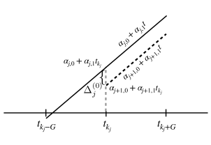
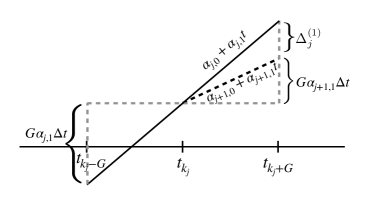
Figure 3: Left: the slope of $f_{i}$ remains unchanged while a discontinuous jump occurs at $t_{k_{j}}$. Right: the slope of $f_{i}$ changes but the signal remains continuous. In both plots, linear curves corresponding to the pre- and the post-change parameters are given in solid and dashed lines, respectively, and the size of $\Delta_{j}^{(0)}$ (left) and $\Delta_{j}^{(1)}$ (right) is highlighted.

1. $\min_{0\leq j\leq J_{n}}|k_{j+1}-k_{j}|>2G$.

2. $(\log(n/G))^{-1/2}\sqrt{G}\min_{1\leq j\leq J_{n}}\|\boldsymbol{\Delta}_{j}\|\to\infty$ as $n\to\infty$.

Assumption (C1) requires that the bandwidth $G$ does not exceed half the distance between any two adjacent change points. Provided that (C1) is met, we permit $J_{n}\to\infty$ as $n\to\infty$. Jointly, (C1)–(C2) place a lower bound on the size of changes for their detection, namely

$$\frac{\min_{0\leq j\leq J_{n}}(k_{j+1}-k_{j})\cdot\min_{1\leq j\leq J_{n}}\|\boldsymbol{\Delta}_{j}\|^{2}}{\log(n)}\to\infty.$$ (5)

Then, Theorem 2.2 establishes the consistency of the MOSUM procedure in detecting multiple change points and derives the rate of localization.

Theorem 2.2.

Assume that (A1)–(A2), (B1)–(B2), and (C1)–(C2) are held. Suppose that $G$ satisfies (3) and $\alpha=\alpha_{n}$ is chosen such that

$$\alpha_{n}\to 0\quad\text{and}\quad\log^{-1/2}(n/G)C_{n}(G,\alpha_{n})=O(1).$$ (6)

Then, as $n\to\infty$, the set of change point estimators $\{\widehat{k}_{j},\,j=1,\ldots,\widehat{J}_{n}:\,\widehat{k}_{1}<\ldots<\widehat{k}_{\widehat{J}_{n}}\}$ returned by the MOSUM procedure satisfies:

1. $\Pr\left(\widehat{J}_{n}=J_{n}\text{ and }\max_{1\leq j\leq J_{n}}|\widehat{k}_{j}-k_{j}|<G\right)\to 1$.

2. Additionally, assume that $f_{i}$ is piecewise linear and continuous. Also, we use $\widehat{\tau}_{k}^{2}=\widehat{\tau}^{2}$ which satisfies $\Pr(\widehat{\tau}^{2}>0)\to 1$ and $\widehat{\tau}^{2}=O_{P}(1)$. Then, there exists a fixed constant $c_{0}>0$ such that, for all $c_{0}\leq\xi\leq G$ and $1\leq j\leq J_{n}$, $\Pr\left(|\widehat{k}_{j}\mathbb{I}_{\{j\leq\widehat{J}_{n}\}}-k_{j}|\geq\xi\right)=O\left(d_{j}^{-\gamma}\xi^{-3\gamma/2}\right)+o(1)$, where $d_{j}=|f_{k_{j}+1}-2f_{k_{j}}+f_{k_{j}-1}|=|G^{-1}\Delta^{(1)}_{j}|$.

Theorem 2.2 (i) shows that the MOSUM procedure achieves consistency in estimating $J_{n}$, and it locates a single estimator within the interval of length $G$ from each $k_{j}$. Further, when $f_{i}$ is continuous, (ii) derives the rate of localization, which implies that $\max_{1\leq j\leq J_{n}}d_{j}^{2/3}|\widehat{k}_{j}-k_{j}|=O_{P}(J_{n}^{1/\gamma})$. In particular, when $d_{j}=O(n^{-1})$ (which ensures the boundedness of $f_{i}$) and the number of change points is finite (i.e., $J_{n}=O(1)$), the resultant rate, $\max_{1\leq j\leq J_{n}}|\widehat{k}_{j}-k_{j}|=O_{P}(n^{2/3})$, matches the minimax lower bound derived in Raimondo, (1998) in the context of a single sharp ‘cusp’ estimation (see Theorem 4.6 therein). In Theorem 2.2 (ii), the condition that $\widehat{\tau}_{k}^{2}=\widehat{\tau}^{2}$ is made for the ease of the proof, and this estimator $\widehat{\tau}^{2}$ is required only to be bounded appropriately without being consistent.

Remark 2.2 (Comparison with the existing results).

Our theoretical results are derived under considerably weaker conditions compared to the existing literature. Most notably, we assume that $\mathsf{E}(|\epsilon_{i}|^{\gamma})<\infty$ with some finite $\gamma>2$ only through (A2), whereas it is commonly assumed that $\{\epsilon_{i}\}$ is a sequence of (sub-)Gaussian random variables with the exception of Maeng and Fryzlewicz, (2023), and the latter still requires that all moments of $\epsilon_{i}$ exist. When continuity is imposed on $f_{i}$ (such that $\Delta^{(0)}_{j}=0$), the condition (5) is analogous to those found in Baranowski et al., (2019) (permit diverging $J_{n}$ as in this paper) and Fearnhead et al., (2019) (assume $J_{n}=O(1)$). Also, in this case, the rate of localization obtained in Theorem 2.2 (ii) is comparable to those obtained in the above papers, or even sharper when the number of change points grows slowly as $J_{n}=o(\log(n))$. We mention that Maeng and Fryzlewicz, (2023) and Yu et al., (2022) derived the rate of localization without assuming continuity; we defer the discussion of the case of discontinuous $f_{i}$ to the Supplementary Material.

Remark 2.3 (Variance estimation).

There exist estimators of the variance $\sigma^{2}$ and LRV $\tau^{2}$ that are robust to the presence of multiple mean shifts (Eichinger and Kirch,, 2018; Dette et al.,, 2020; Chan,, 2022; McGonigle and Cho,, 2023), which are combined with the mean change point detection procedures. We propose a MOSUM-based local estimator of LRV that extends the estimator of Eichinger and Kirch, (2018) in Section A.1 and show that it fulfils (B1)–(B2) (Theorem A.1). In the special case of independent $\{\epsilon_{i}\}_{i\in\mathbb{Z}}$ where $\tau^{2}=\sigma^{2}$, the proposed estimator for $k=G,\ldots,n-G$, is

$$\widehat{\sigma}_{k}^{2}=\frac{1}{2}\left(\widehat{\sigma}_{k,-}^{2}+\widehat{\sigma}_{k,+}^{2}\right),\quad\text{where}\quad\widehat{\sigma}_{k,\pm}^{2}=\frac{1}{G-2}\sum_{i\in\mathcal{I}^{\pm}(k)}\left(X_{i}-\widehat{\beta}_{0}^{\pm}{(k)}-\frac{i-k}{G}\widehat{\beta}_{1}^{\pm}{(k)}\right)^{2}.$$ (7)

Remark 2.4.

When $f_{i}$ is piecewise linear and continuous, the quantity $\widetilde{W}_{k}(G)=\|\boldsymbol{\Sigma}^{-1/2}[\boldsymbol{\beta}^{+}(k)-\boldsymbol{\beta}^{-}(k)]\|$ (where $\boldsymbol{\beta}^{\pm}(k)$ is obtained by regressing $f_{i}$ on $\mathbf{x}_{i,k}$) attains a single local maximum at each $k_{j}$, which leads to the desirable behaviour of $W_{k,n}(G)$ observed in Figure 2 and the localization property in Theorem 2.2 (ii). If $f_{i}$ is discontinuous (i.e., $\Delta_{j}^{(0)}\neq 0$), $\widetilde{W}_{k}(G)$ attains multiple peaks within the interval $\{k_{j}-G+1,\ldots,k_{j}+G\}$ and, although one peak is located at $k_{j}$, it is not necessarily the local maximizer. However, combined with the local variance estimator proposed in (7), the statistic $W_{k,n}(G)$ tends to attain clear local maxima at the true change points due to the upward bias in $\widehat{\sigma}_{k}^{2}$ at $k\neq k_{j}$, and hence, performs well empirically. See Section A.2 for further discussions, and Section 3.3 for how this behaviour may be exploited for the diagnosis of the types of changes.

3 Numerical considerations

3.1 Computational complexity

The computational complexity of the proposed MOSUM procedure is $O(n)$. This is due to the sequential update available for the coefficient estimators $\widehat{\boldsymbol{\beta}}^{\pm}(k)$ and the local variance estimator in (7), see Section B.2 for the updating equations. In Section 4.2, we numerically demonstrate the competitiveness of the proposed MOSUM procedure, where it takes a fraction of the time taken for other methods to process large datasets.

3.2 Multiscale extension

If the bandwidth $G$ is chosen too small, the MOSUM procedure may lack detection power, while when $G$ is too large, the violation of the condition (C1) makes it difficult to detect or locate change points which are close to one another. Generally, it is well-recognized in the literatures that a moving window-type procedure applied with a single bandwidth lacks adaptivity. One remedy is to apply the procedure with multiple bandwidths, say $\mathcal{G}=\{G_{b},\,1\leq b\leq B:\,G_{1}<\ldots<G_{B}\}$ and prune down the set of estimators to remove any duplicate estimators. Let $\widehat{\mathcal{K}}_{b}=\{\widehat{k}_{b,j},\,1\leq j\leq\widehat{J}_{b}\}$ denote the set of estimators obtained with $G_{b}$ as the bandwidth, where $\widehat{k}_{b,j}$ are ordered in the decreasing order of the corresponding MOSUM statistic, i.e., $W_{\widehat{k}_{b,1},n}(G_{b})\geq W_{\widehat{k}_{b,2},n}(G_{b})\geq\ldots\geq W_{\widehat{k}_{b,\widehat{J}_{b}},n}(G_{b})$. Supposing that the bandwidths are sorted according to some measure of importance as $G_{\pi(b)},\,b=1,\ldots,B$, we propose to sequentially accept $\widehat{k}_{j,\pi(b)}$ for $j=1,\ldots,\widehat{J}_{\pi(b)}$ and $b=1,\ldots,B$, to the set of final estimators $\widehat{\mathcal{K}}$ if $\widehat{k}_{j,\pi(b)}$ is sufficiently distanced away from the already accepted estimators. That is, starting with $\widehat{\mathcal{K}}=\emptyset$, we check whether $\min_{\widehat{k}\in\widehat{\mathcal{K}}}|\widehat{k}_{j,\pi(b)}-\widehat{k}|>\theta G_{\pi(b)}$ for increasing $j$ and $b$, with a pre-determined constant $\theta\in(0,1]$, and if so, accepts $\widehat{k}_{j,\pi(b)}$ to $\widehat{\mathcal{K}}$ (with the convention $\min\emptyset=\infty$).

When the bandwidths are sorted in the increasing order such that $G_{\pi(b)}=G_{b}$, this coincides with the bottom-up merging proposed by Messer et al., (2014). Instead, we propose to adopt the Bayesian information criterion ${\rm BIC}(\mathcal{K})=n\log\left(\frac{{\rm RSS}(\mathcal{K})}{n}\right)+2\big{(}|\mathcal{K}|+1\big{)}\log(n)$ for bandwidth sorting, where ${\rm RSS}(\mathcal{K})$ denotes the residual sum of squares of the model fitted under (1) with $\mathcal{K}$ as the set of change points. Then, we find $\pi(\cdot)$ satisfying ${\rm BIC}(\widehat{\mathcal{K}}(G_{\pi(1)}))\leq{\rm BIC}(\widehat{\mathcal{K}}(G_{\pi(2)}))\leq\ldots\leq{\rm BIC}(\widehat{\mathcal{K}}(G_{\pi(B)}))$. Although not reported here, we numerically examined the use of alternative information criteria such as AIC and the cross-validation measure of Zou et al., (2020), which performed similarly well as the proposed BIC-based sorting. On the other hand, the bottom-up merging tends to produce more false positives and attain poorer localization accuracy by preferring the estimators from the finer bandwidths, a phenomenon also observed by Cho and Kirch, 2022b in the context of the univariate mean change point detection problem. Investigating whether the results reported in Theorem 2.2 extend to the multiscale procedure is interesting, but it is beyond the scope of this paper, which we leave for future research.

3.3 Practical issues in implementation

Critical value.

The theoretically motivated critical value $C_{n}(G,\alpha)$ given in Section 2.2.1 requires the selection of $\alpha$. In view of the condition on $\alpha$ in (6), we use $\alpha=0.05$ throughout this paper. It also involves some unknown constant $H$ through $b_{G}$, which we set $\log(H)\approx 0.7284$ based on extensive numerical experiments, see Section B.1 for details.

Bandwidths.

For the multiscale MOSUM procedure described in Section 3.2, we use a set of bandwidths $\{G_{1},\ldots,G_{B}\}$ generated as a Fibonacci sequence following Cho and Kirch, 2022b . Namely, for given $G_{0}=G_{1}$, we generate $G_{b}=G_{b-1}+G_{b-2}$ for $b\geq 2$ until $G_{B+1}$ exceeds $n/\log_{10}(n)$ while $G_{B}<n/\log_{10}(n)$. In view of the condition (3), we adopt $G_{1}=10$ ($n=500$) or $G_{1}=50$ ($n=2500,3500$) in simulation studies and $G_{1}=100$ for real data analysis, which are set to be greater than $0.01n$ for the sample size in consideration.

Tuning parameters $\eta$ and $\theta$.

In our numerical experiments, varying the value of $\eta$ used in the estimation rule does not lead to noticeably different performance within the range $\eta\in[0.2,0.4]$, and a similar conclusion is drawn for the choice of $\theta$ adopted in the multiscale extension, provided that $\theta\geq 0.8$. As a rule of thumb, we recommend $(\eta,\theta)=(0.3,0.8)$, since choosing too large values for these parameters may prevent detection of some change points.

Diagnostic.

Investigating whether a change relates to a continuous change in the slope ($\Delta_{j}^{(0)}=0$) or a discontinuous jump (due to a change of the intercept, $\Delta_{j}^{(0)}\neq 0$) can be interesting in practice. For this purpose, we can adopt the visualization of the MOSUM statistics $W_{k,n}(G)$ as a diagnostic tool, based on the fact that $W_{k,n}(G)$ behaves differently around the change point $k_{j}$ depending on the values of $\Delta_{j}^{(0)}$ and $\Delta_{j}^{(1)}$, i.e., $W_{k,n}(G)$ has unimodal peak around $k_{j}$ only when $\Delta_{j}^{(0)}=0$. We provide further illustrative examples in Section A.2.

4 Numerical experiments

4.1 Simulation studies

Data generation.

We consider the following different scenarios for the generation of $f_{i}$: (M0) no change point ($J=0$), (M1) piecewise linear with three change points ($J=3$), (M2) piecewise linear and continuous with $J=3$, (M3) piecewise linear with $J=6$, and (M4) piecewise constant with $J=3$. We have $n=3500$ under (M0)–(M2) and (M4), while $n=2500$ under (M3). See Section C for a detailed description, which also reports results obtained with a shorter sample size ($n=500$). In all cases, we have $t_{i}=0.01i$. We note that the sample sizes are comparable to those of Baranowski et al., (2019) and Maeng and Fryzlewicz, (2023). For the generation of $\{\epsilon_{i}\}_{i=1}^{n}$, we consider a sequence of i.i.d. random variables with (E1) Gaussian, (E2) scaled $t_{5}$, (E3) scaled Laplace distributions, as well as (E4) an AR process: $\epsilon_{i}=\rho\epsilon_{i-1}+\sqrt{1-\rho^{2}}\sigma Z_{i}$ with $\rho\in\{0.3,0.7\}$ and $Z_{i}\sim_{\text{i.i.d.}}\mathcal{N}(0,1)$. We vary $\mathsf{Var}(\epsilon_{i})=\sigma^{2}$ with $\sigma\in\{0.5,1,1.5,2\}$, but only report the results with $\sigma=1$ in the main text unless specified otherwise; see Section C.2 for the full results.

Tuning parameters and competitors.

We apply the multiscale extension of the MOSUM procedure, referred to as ‘MOSUM’ below. The tuning parameters, including the set of bandwidths, are chosen as described in Section 3.3. Also, unless stated otherwise, we use the MOSUM-based local estimator of variance given in (7) as $\widehat{\tau}_{k}$. For comparison, we include the narrowest-over-threshold method proposed by Baranowski et al., (2019), the $\ell_{0}$-penalized least squares estimation method of Fearnhead et al., (2019), and the wavelet-based method of Maeng and Fryzlewicz, (2023), referred to as NOT.pwLin [R package not], CPOP [R package cpop] and TGUW [R package trendsegmentR], respectively. NOT.pwLin takes as an input whether $f_{i}$ is continuous and accordingly, we separately report the results from NOT.pwLin with the continuity imposed (NOT.pwLinCont). These are applied along with the recommended default tuning parameters.

Performance metrics.

For each setting, we report the results from $1000$ replications according to the following measures of performance. Let $\mathcal{K}=\{t_{k_{j}},\,1\leq j\leq J:\,k_{1}<\cdots<k_{J}\}$ denote the set of true change points, and $\widehat{\mathcal{K}}=\{t_{\widehat{k}_{j}},\,1\leq j\leq\widehat{J}:\,\widehat{k}_{1}<\cdots<\widehat{k}_{\widehat{J}}\}$ the set of change point estimators. Then, we compute $\text{{COUNTscore}}=|\widehat{J}-J|$, $\text{{MAXscore1}}=\max_{1\leq j\leq J}\min_{1\leq j^{\prime}\leq\widehat{J}}|t_{\widehat{k}_{j^{\prime}}}-t_{k_{j}}|$ and $\text{{MAXscore2}}=\max_{1\leq j^{\prime}\leq\widehat{J}}\min_{1\leq j\leq J}|t_{\widehat{k}_{j^{\prime}}}-t_{k_{j}}|$. COUNTscore evaluates the accuracy in estimating $J$, and MAXscore1 and MAXscore2 assess both detection and localization accuracy. MAXscore1 is large when a true change point is undetected (false negative), while MAXscore2 is large when a spurious estimator is detected far from true change points (false positive). For all three, smaller values indicate better performance.

Results.

Table 1 shows that the proposed MOSUM procedure accurately estimates the total number and locations of the change points. Applied to the datasets generated under (M1)–(M3), MOSUM performs as well as, or slightly outperforms, NOT.pwLin regardless of the error distribution or the types of changes and their frequency. TGUW tends to perform worse than MOSUM or NOT.pwLin in all settings, both in terms of detection and estimation accuracy, and its performance deteriorates much more severely when the errors are generated from heavy-tailed distributions under (E2)–(E3). NOT.pwLinCont and CPOP pre-suppose that the signals are piecewise linear and continuous, and as such, they perform well under (M2) but poorly in other scenarios, and tend to over-estimate the number of change points by detecting spurious estimators in order to approximate the discontinuous signal by introducing additional segments (see Table C.1 and Figure C.2). The detection performance of MOSUM under (M2) is not far behind NOT.pwLinCont and slightly better than NOT.pwLin. Also, in this scenario, the localization accuracy measured by MAXscore1 and MAXscore2 becomes worse in the presence of heavy-tailed errors for all methods. Under (M3), the signal has frequent change points ($J=6$) and the distance between adjacent change points is shorter; the smallest distance between change points is $100$ in comparison with $500$ under (M1)–(M2). Here, MOSUM is still highly competitive and outperforms the competitors in estimation accuracy, particularly when the data is heavy-tailed.

Table 2 concerns the case of serially correlated errors generated under (E4). We consider two approaches: (i) we continue to use the variance estimator in (7) for calibration (‘MOSUM’) with ignoring the serial dependence, and (ii) we use the difference-based estimator of the LRV proposed in Chan, (2022) obtained from the entire sample (‘MOSUM.dlrv’). In the presence of weak serial dependence ($\rho=0.3$), MOSUM does reasonably well in not returning spurious estimators. However, when the serial dependence becomes stronger with $\rho=0.7$, such an approach suffers from the calibration issue, for which MOSUM.dlrv provides a reasonably good solution. Even so, the performance is worse than the independent setting as the signal-to-noise ratio decreases with increasing $\rho$. The implementation of NOT.pwLin do not permit the user to supply an alternative scaling parameter, and the default choice fails to adequately suppress the spurious false positives; TGUW also performs worse although its implementation accommodates serial dependence.

Table 3 considers the case when the signal is piecewise constant with $\alpha_{1,j}=0$ in (1). Here, we additionally consider NOT.pwConst (‘piecewise constant’) as proposed in Baranowski et al., (2019) besides MOSUM, NOT.pwLin, and TGUW. The MOSUM procedure shows comparable or better performance than NOT.pwConst regardless of $n$ when the noise level is small ($\sigma=1$), but its performance deteriorates when $\sigma=2$. Due to increased noise level, MOSUM sometimes approximates the signal with three linear segments rather than two constant segments around $k_{1}$ (see Figure C.3).

Finally, we examine the performance of different methods when no change point is present ($J=0$), see Table 4. We observe that MOSUM successfully avoids detecting any spurious estimators in almost all realizations, even when the data is heavy-tailed under (E2)–(E3). NOT-based methods work well even when $\epsilon_{i}$ is not Gaussian, and generally, NOT.pwLinCont is more conservative than NOT.pwLin. CPOP and TGUW suffer greatly when the error distribution is heavy-tailed, and the former, in particular, detects a large number of false positives.

Table 1: (M1)–(M2) with $J=3$ and $n=3500$ and (M3) with $J=6$ and $n=2500$. Results from MOSUM, NOT.pwLin, NOT.pwLinCont, CPOP and TGUW when the errors are generated as in (E1)–(E3) with $\sigma=1$. We report the average and standard error (in parentheses) of the performance metrics over $1000$ realizations.

Model	Error	Metric	MOSUM	NOT.pwLin	NOT.pwLinCont	CPOP	TGUW
(M1)	(E1)	COUNTscore	0.001 (0.0316)	0.003 (0.0547)	–	–	0.029 (0.1679)
		MAXscore1	0.088 (0.0601)	0.123 (0.0653)	–	–	0.152 (0.1142)
		MAXscore2	0.093 (0.1545)	0.131 (0.2561)	–	–	0.158 (0.1386)
	(E2)	COUNTscore	0 (0)	0.023 (0.1962)	–	–	0.472 (1.1741)
		MAXscore1	0.083 (0.0574)	0.117 (0.0657)	–	–	0.172 (0.1219)
		MAXscore2	0.083 (0.0574)	0.184 (0.776)	–	–	0.84 (1.9763)
	(E3)	COUNTscore	0 (0)	0.002 (0.0632)	–	–	0.64 (1.3506)
		MAXscore1	0.083 (0.0582)	0.117 (0.0664)	–	–	0.176 (0.1259)
		MAXscore2	0.083 (0.0582)	0.124 (0.2406)	–	–	1.155 (2.3102)
(M2)	(E1)	COUNTscore	0 (0)	0 (0)	0 (0)	0.003 (0.0547)	0.069 (0.2652)
		MAXscore1	0.186 (0.0883)	0.262 (0.1016)	0.047 (0.0253)	0.05 (0.0261)	0.372 (0.1817)
		MAXscore2	0.186 (0.0883)	0.262 (0.1016)	0.047 (0.0253)	0.054 (0.0969)	0.393 (0.2488)
	(E2)	COUNTscore	0.003 (0.0547)	0.019 (0.1633)	0.004 (0.0632)	5.989 (4.1427)	0.659 (1.237)
		MAXscore1	0.336 (0.5639)	0.454 (0.5608)	0.123 (0.5478)	0.204 (0.3175)	0.751 (0.6129)
		MAXscore2	0.306 (0.1857)	0.482 (0.728)	0.102 (0.311)	4.634 (3.2025)	1.501 (1.9696)
	(E3)	COUNTscore	0.002 (0.0447)	0.016 (0.1542)	0.002 (0.0447)	3.606 (3.3289)	0.866 (1.443)
		MAXscore1	0.314 (0.4752)	0.424 (0.4657)	0.111 (0.4489)	0.168 (0.3693)	0.747 (0.5885)
		MAXscore2	0.294 (0.182)	0.433 (0.4659)	0.092 (0.0677)	3.221 (3.3163)	1.761 (2.2033)
(M3)	(E1)	COUNTscore	0 (0)	0.003 (0.0547)	–	–	0.196 (0.5328)
		MAXscore1	0.182 (0.0943)	0.244 (0.0965)	–	–	0.319 (0.1676)
		MAXscore2	0.182 (0.0943)	0.248 (0.1671)	–	–	0.433 (0.4911)
	(E2)	COUNTscore	0 (0)	0.025 (0.1685)	–	–	0.485 (0.9406)
		MAXscore1	0.18 (0.0917)	0.239 (0.1029)	–	–	0.384 (0.1921)
		MAXscore2	0.18 (0.0917)	0.248 (0.1997)	–	–	0.607 (0.6723)
	(E3)	COUNTscore	0 (0)	0.007 (0.0947)	–	–	0.518 (1.0221)
		MAXscore1	0.177 (0.0976)	0.244 (0.0999)	–	–	0.392 (0.1863)
		MAXscore2	0.177 (0.0976)	0.251 (0.203)	–	–	0.646 (0.7245)

Table 2: (M1) with $J=3$ and $n=3500$. Results from the MOSUM, MOSUM.dlrv (MOSUM applied with the LRV estimator of Chan, (2022)), NOT.pwLin and TGUW when the errors are generated as in (E4) with $\sigma=1$. We report the average and standard error (in parentheses) of the performance metrics over $1000$ realizations.

$\rho$	Metric	MOSUM	MOSUM.dlrv	NOT.pwLin	TGUW
$0.3$	COUNTscore	0.044 (0.2369)	0.492 (0.5237)	0.123 (0.4517)	2.236 (2.1272)
	MAXscore1	0.101 (0.0686)	0.44 (0.3841)	0.142 (0.0795)	0.171 (0.1247)
	MAXscore2	0.24 (0.8439)	0.658 (0.5796)	0.442 (1.3325)	3.403 (3.1662)
$0.7$	COUNTscore	8.233 (2.8791)	0.72 (0.5549)	12.368 (6.1324)	123.405 (10.9049)
	MAXscore1	0.151 (0.1231)	0.558 (0.3844)	0.219 (0.1727)	0.104 (0.095)
	MAXscore2	7.594 (1.5732)	0.953 (0.5848)	7.784 (2.2462)	9.806 (0.1351)

Table 3: (M4) with $J=3$ and $n=3500$. Results from MOSUM, NOT.pwLin, NOT.pwConst, and TGUW when the errors are generated as in (E1) with $\sigma\in\{1,2\}$. We report the average and standard error (in parentheses) of the performance metrics over $1000$ realizations.

$\sigma$	Metric	MOSUM	NOT.pwLin	NOT.pwConst	TGUW
$1$	COUNTscore	0 (0)	0.001 (0.0316)	0.008 (0.0891)	0.073 (0.2603)
	MAXscore1	0.001 (0.0026)	0.001 (0.0026)	0.001 (0.0026)	0.006 (0.0131)
	MAXscore2	0.001 (0.0026)	0.001 (0.0048)	0.035 (0.4835)	0.008 (0.0185)
$2$	COUNTscore	0.162 (0.382)	0 (0)	0.019 (0.1366)	0.263 (0.4879)
	MAXscore1	0.121 (0.2746)	0.007 (0.0108)	0.007 (0.011)	0.049 (0.0761)
	MAXscore2	0.155 (0.3468)	0.007 (0.0108)	0.062 (0.5403)	0.068 (0.1884)

Table 4: (M0) with $J=0$ and $n=3500$. Results from the MOSUM, NOT.pwLin, NOT.pwLinCont, CPOP and TGUW when the errors are generated as in (E1)–(E3). We report the average and standard error (in parentheses) of COUNTscore over $1000$ realizations.

Error	$\sigma$	MOSUM	NOT.pwLin	NOT.pwLinCont	CPOP	TGUW
(E1)	$0.5$	0 (0)	0 (0)	0 (0)	0.002 (0.0447)	0.002 (0.0632)
	$1$	0 (0)	0 (0)	0 (0)	0 (0)	0 (0)
	$1.5$	0.001 (0.0316)	0 (0)	0.001 (0.0316)	0.001 (0.0316)	0 (0)
	$2$	0 (0)	0 (0)	0 (0)	0 (0)	0 (0)
(E2)	$0.5$	0 (0)	0.022 (0.2039)	0 (0)	5.668 (4.1193)	0.572 (1.5822)
	$1$	0 (0)	0.021 (0.1913)	0.001 (0.0316)	5.993 (4.1367)	0.516 (1.5219)
	$1.5$	0 (0)	0.008 (0.1482)	0 (0)	5.883 (4.2099)	0.558 (1.5694)
	$2$	0 (0)	0.015 (0.1637)	0.002 (0.0632)	5.773 (4.2525)	0.62 (1.7054)
(E3)	$0.5$	0 (0)	0.01 (0.1411)	0 (0)	3.362 (3.4004)	0.849 (1.9764)
	$1$	0 (0)	0.017 (0.1864)	0 (0)	3.397 (3.2376)	0.904 (1.9567)
	$1.5$	0 (0)	0.013 (0.1577)	0 (0)	3.184 (3.0465)	0.859 (1.9367)
	$2$	0 (0)	0.004 (0.0894)	0 (0)	3.292 (3.2477)	0.754 (1.8409)

4.2 Execution time

We report the average execution time of different methods when applied to $100$ realizations generated under (M1) with $n=3500$ and i.i.d. Gaussian errors as in (E1). See Table 5. The sequential update available for the MOSUM statistics makes the computational complexity of the proposed method very low (see Section B.2). The single-bandwidth MOSUM procedure requires less than $1$ ms. When applied with the set of bandwidths $\mathcal{G}$ chosen as described in Section 3.2 with $|\mathcal{G}|=6$, the multiscale extension still requires less than $5$ ms on average. In contrast, NOT.pwLin and NOT.pwLinCont are much slower, with the average execution time exceeding $200$ ms. Their performance is followed by TGUW, and the dynamic programming-based CPOP takes more than $20$ seconds for its execution. This demonstrates the computational advantage of the MOSUM procedure, particularly when the datasets are long. Although not reported here, similar observations are made across different simulation scenarios.

Table 5: Average execution time (in milliseconds) of change point detection methods over 100 realizations generated as in (M1) ($n=3500$). All experiments are conducted on R 4.2.1 with the processor of 2100MHz 12-core i7-1260P and 16GB of memory.

	MOSUM ($G=200$)	MOSUM (multiscale)	NOT		CPOP	TGUW
			pwLin	pwLin.Cont
Time (ms)	0.685	3.853	187.88	521.55	$>2\times 10^{4}$	1843.37

5 Real data analysis

We analyze a time series dataset described in the Introduction, which is of length $n=9830$. See Figure 1. We apply the multiscale extension of the MOSUM procedure described in Section 3.2 with the set of bandwidths $\mathcal{G}=\{100,200,300,500,800,1300,2100\}$. The estimated change points are shown in the top panel of Figure 4, along with the estimator of the piecewise linear signal. There are $19$ change points detected, and many of them are detected after February 16th. Although omitted here, there is little autocorrelation left in the residuals from the piecewise linear fit to the data, which supports using a MOSUM-based variance estimator in (7) rather than an estimator of LRV.

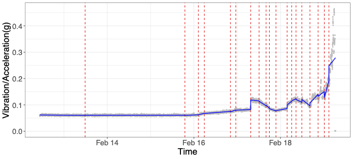
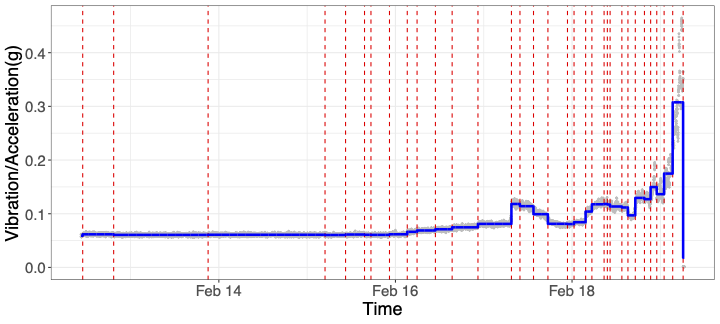
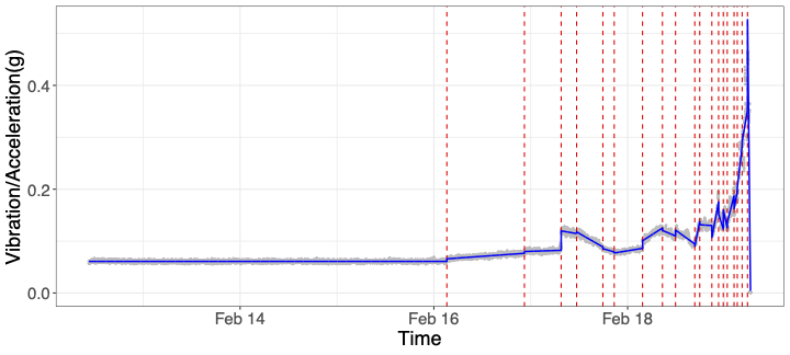
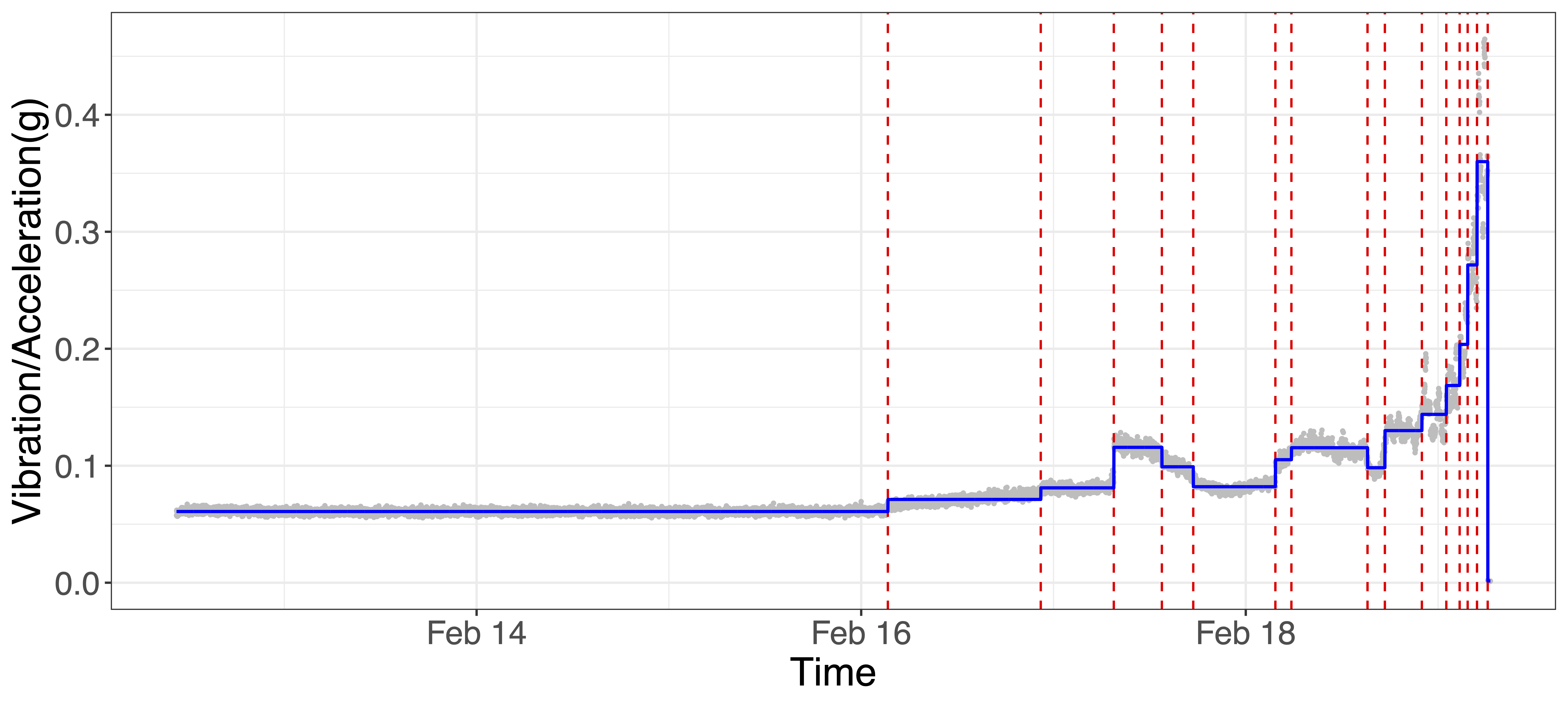
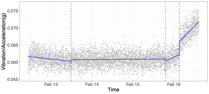
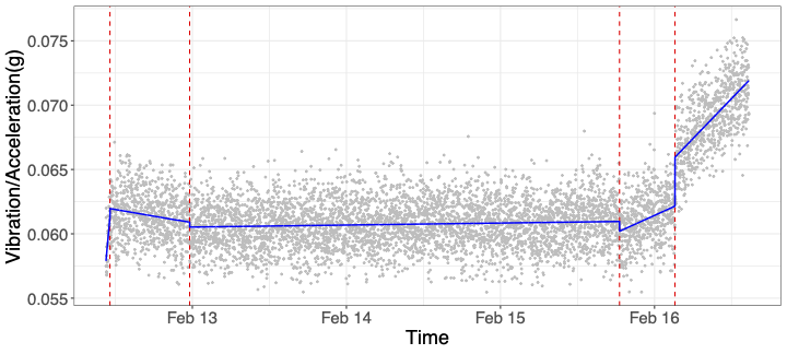
Figure 4: Bearing dataset superimposed with the change points detected by different methods (vertical broken lines) and the estimated piecewise linear signal (solid). We visualize the results from MOSUM (top left), MOSUM.pwConst (top right), NOT.pwLin (middle left) and NOT.pwConst (middle right). At bottom, change points detected from the truncated bearing dataset by the proposed MOSUM procedure (left) and NOT.pwLin (right) are displayed.

For comparison, we apply NOT.pwLin and the methods which detect change points under piecewise constant modeling, such as NOT.pwConst, the variant of NOT (see Table 3), and MOSUM.pwConst, the multiscale MOSUM procedure combined with the bottom-up merging as implemented in Meier et al., (2021); we apply the latter with $\mathcal{G}$ as the set of bandwidths. Figure 4 shows that MOSUM.pwConst detects more change points than our method, possibly as it tries to approximate a signal with trends using a piecewise constant signal. Both NOT.pwLin and NOT.pwConst do not detect any change point before February 16th while detecting more frequent change points post-February 17th. These differences are attributed to the variability increasing significantly towards the end of the signal. NOT-based methods use a single constant as an estimator of the noise level, which may have been chosen too large to detect the subtle changes before February 16th, while too small to prevent these methods from possibly over-fitting the anomalous behavior post-February 17th. On the other hand, by adopting the local variance estimator in (7), the proposed MOSUM procedure better captures local variability. We further verify this by considering the truncated dataset which runs up to about 3 PM on February 16th ($n=6000$), see bottom panels of Figure 4. As desired, the truncation of the data does not alter the results reported by our method whereas NOT.pwLin returns estimators previously undetected when applied to the entire dataset. This also demonstrates the applicability of the MOSUM procedure for real-time monitoring of change points.

6 Concluding remarks

This paper introduces a moving sum-based methodology for detecting multiple changes in both intercept and slope parameters under a piecewise linear model. We derive the asymptotic null distribution of the proposed Wald-type MOSUM test statistic, which provides a principled way of calibrating the methodology while controlling the family-wise error. We also establish its theoretical consistency in multiple change point detection and, when the additional continuity is imposed, derive the rate of localization. In doing so, we make a mild assumption on the errors, which is considerably weaker than independence and (sub-)Gaussianity assumptions found in the relevant literature. The competitiveness of the proposed methodology is further demonstrated empirically on both simulated and real datasets compared to the existing methods, where it shows promising performance thanks to the adoption of moving windows that enables efficient computation with $O(n)$ complexity. We envision that the proposed methodology and tools for theoretical analysis can be generalized to detect multiple change points under piecewise polynomial models.

Appendix A Supplements for the theoretical results

A.1 Estimation of long-run variance

We proposed a MOSUM-based local estimator of variance $\sigma^{2}$ under independence in the manuscript, see Remark 2.3. In this section, we propose a local long-run variance (LRV) estimator that extends the estimator of Eichinger and Kirch, (2018) to our setting, and establish its properties under serial dependence.

Denote by $\Gamma(h)=\mathsf{Cov}(\epsilon_{0},\epsilon_{h})$ the autocovariance (ACV) function of $\{\epsilon_{i}\}$ at lag $h$, such that $\tau^{2}=\sigma^{2}+2\sum_{h=1}^{\infty}\Gamma(h)$. Then we propose a MOSUM-based local ACV estimator $\widehat{\Gamma}_{k}(h)=(\widehat{\Gamma}_{k,+}(h)+\widehat{\Gamma}_{k,-}(h))/2$, where

$$\widehat{\Gamma}_{k,+}(h) =\frac{1}{G-2}\sum_{i=k+1}^{k+G-h}\big{(}X_{i}-\mathbf{x}_{i,k}^{\top}\widehat{\boldsymbol{\beta}}^{+}(k)\big{)}\big{(}X_{i+h}-\mathbf{x}_{i+h,k}^{\top}\widehat{\boldsymbol{\beta}}^{+}(k)\big{)}\text{ \ and \ }$$

$$\widehat{\Gamma}_{k,-}(h) =\frac{1}{G-2}\sum_{i=k-G+1}^{k-h}\big{(}X_{i}-\mathbf{x}_{i,k}^{\top}\widehat{\boldsymbol{\beta}}^{-}(k)\big{)}\big{(}X_{i+h}-\mathbf{x}_{i+h,k}^{\top}\widehat{\boldsymbol{\beta}}^{-}(k)\big{)},$$

with estimating $\tau^{2}$ by $\widehat{\tau}_{k}^{2}=\widehat{\Gamma}_{k}(0)+2\sum_{h=1}^{S_{n}}\mathcal{K}(h/S_{n})\widehat{\Gamma}_{k}(h)$. Here $\mathcal{K}(\cdot)$ is a bounded kernel such as the flat-top (Politis and Romano,, 1995) or Bartlett kernels, and $S_{n}$ denotes the kernel bandwidth. If we additionally assume that $\{\epsilon_{i}\}$ is a sequence of i.i.d. random variables, it suffices to estimate the variance $\sigma^{2}$ by $\widehat{\sigma}_{k}^{2}=\widehat{\Gamma}_{k}(0)$, which becomes (7) in the manuscript.

Theorem A.1 establishes that under weak dependence, $\widehat{\tau}_{k}^{2}$ fulfils the first condition in (B1). Some kernel-based LRV estimators are not guaranteed to be positive, in which case a standard solution is to truncate the estimator from the below, and we may similarly enforce the boundedness from the above. Under independence, $\widehat{\sigma}_{k}^{2}$ satisfies both (B1) and (B2) without such truncation.

Theorem A.1.

Assume that $\{\epsilon_{i}\}_{i\in\mathbb{Z}}$ satisfies (A1) and $\mathsf{E}(|\epsilon_{1}|^{4})<\infty$, and the bandwidth $G$ satisfies (3). Furthermore, assume that $\sup_{h\in\mathbb{Z}}\sum_{k\in\mathbb{Z}}\sum_{\ell\in\mathbb{Z}}|\omega(h,k,\ell)|<\infty$, where $\omega(h,k,\ell)=\mathsf{Cov}(\epsilon_{1}\epsilon_{1+h},\epsilon_{1+k}\epsilon_{1+\ell})$.

1. If $0\leq\mathcal{K}(x)\leq C$ for some constant $C\in(0,\infty)$ and $G^{-2}S_{n}^{2}n=O(1)$, uniformly over all $k$ satisfying $\min_{1\leq j\leq J_{n}}|k-k_{j}|\geq G$, we have

   $$\big{|}\widehat{\tau}_{k}^{2}-\tau^{2}\big{|}=O_{P}\left(\frac{\sqrt{n}S_{n}}{G}+\sum_{h\in\mathbb{Z}}\left|\mathcal{K}\left(\frac{h}{S_{n}}\right)-1\right|{|\Gamma(h)|}\right).$$

2. Additionally, suppose that $\{\epsilon_{i}\}_{i\in\mathbb{Z}}$ is a sequence of i.i.d. random variables.

   1. Uniformly over all $k$ satisfying $\min_{1\leq j\leq J_{n}}|k-k_{j}|\geq G$, we have

      $$\left|\widehat{\sigma}_{k}^{2}-\sigma^{2}\right|=o_{P}\left(\frac{1}{\log(n/G)}\right)\quad\text{and}\quad\widehat{\sigma}_{k}^{-2}=O_{P}(1).$$

   2. $\max_{G\leq k\leq n-G}\widehat{\sigma}_{k}^{2}=O_{P}(1)$, provided that $\max_{1\leq j\leq J_{n}}\|\boldsymbol{\Delta}_{j}\|=O(1)$.

Proof of the theorem is in Section D.

A.2 When $f_{i}$ is piecewise linear and discontinuous

In this section, we explore the behavior of the Wald-type MOSUM statistic $W_{k,n}(G)$ in (2) when $f_{i}$ is not necessarily continuous.

For $k\in\{k_{j}-G+1,\ldots,k_{j}+G\}$, we can approximate $\mathsf{E}[\widehat{\boldsymbol{\beta}}^{+}(k)-\widehat{\boldsymbol{\beta}}^{-}(k)]$ by

$$\boldsymbol{\delta}_{j}(\kappa)=(1-|\kappa|)\begin{bmatrix}1-3|\kappa|&\kappa(1-|\kappa|)\\ -6\kappa&-2|\kappa|^{2}+|\kappa|+1\end{bmatrix}\boldsymbol{\Delta}_{j},\text{ \ where \ }\kappa=\frac{k-k_{j}}{G}.$$

See Lemma D.8 in Section D. For $\kappa\in(-1,1]$, we define

$$g_{j}(\kappa)=\sqrt{\left(\boldsymbol{\delta}_{j}(\kappa)\right)^{\top}\begin{bmatrix}1&0\\ 0&\frac{1}{3}\end{bmatrix}\boldsymbol{\delta}_{j}(\kappa)},$$

where the weight matrix is proportional to $\boldsymbol{\Sigma}^{-1}$. When $f_{i}$ is piecewise linear and continuous such that $\Delta^{(0)}_{j}=0$, it further simplifies to $g_{j}(\kappa)=(1-|\kappa|)^{2}\sqrt{|\kappa|^{2}+(2|\kappa|+1)^{2}/3}|\Delta^{(1)}_{j}|$, which has its maximum attained at $\kappa=0$. In short, when $f_{i}$ is continuous, the ‘signal’ part of $W_{k,n}(G)$ forms local maxima at the true change points under (C1).

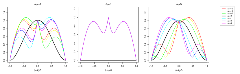
Figure A.1: Behavior of $g_{j}(\kappa)/g_{j}(0),\,\kappa\in(-1,1]$, when $\Delta^{(1)}_{j}=-1$ (left), $\Delta^{(1)}_{j}=0$ (middle) and $\Delta^{(1)}_{j}=5$ (right) and $\Delta^{(0)}_{j}\in\{-3,-2,\ldots,3\}$. In each plot, the curve corresponding to $\Delta^{(0)}_{j}=0$ is highlighted in bold. We adopt the convention $0/0=0$ in the case where $g_{j}(\kappa)\equiv 0$ for all $\kappa$.

The behavior of $g_{j}(\kappa)$ becomes more complex when $f_{i}$ contains discontinuities as illustrated in Figure A.1, which plots the ratio $g_{j}(\kappa)/g_{j}(0)$ for varying combinations of $\boldsymbol{\Delta}_{j}=(\Delta_{j}^{(0)},\Delta^{(1)}_{j})$. When either $\Delta^{(0)}_{j}=0$ or $\Delta^{(1)}_{j}=0$, the ratio is maximized at $\kappa=0$ and in the latter case, $g_{j}(\kappa)$ is unimodal. However, this no longer holds when $\Delta^{(0)}_{j}\neq 0$ and in fact, $g_{j}(\kappa)$ has its maximum anywhere within $\kappa\in(-1,1]$. Due to this, in the absence of continuity, we cannot derive the refined rate of localization for the change point estimators as in Theorem 2.2 (ii), although the proposed MOSUM procedure achieves consistency in detecting the presence of multiple change points regardless of whether $\Delta^{(0)}_{j}=0$ or not. To the best of our knowledge, this characteristic of the Wald-type MOSUM statistic under piecewise linearity has previously been unobserved. We envision that once a change point is detected, its location can further be refined as in Chen, (2021) or Yu et al., (2022) where in particular, the former proposes an estimator that adapts to the unknown regime.

In practice, we benefit from using the proposed local variance estimator in (7), see Figure A.2. Here, we generate $X_{i}$ under (1) with $n=3500$, $\Delta t=0.01$ and $\epsilon_{i}\sim_{\text{i.i.d}}\mathcal{N}(0,0.1^{2})$; for the purpose of illustration, we choose the small error variance so that the data sequence is close to being noiseless. The underlying signal $f_{i}$ is piecewise linear and undergoes three discontinuous jumps at $k_{1}=1000$, $k_{2}=2000$ and $k_{3}=2500$. The middle panel plots $W_{k,n}(G)$ obtained with $G=200$ and the local variance estimator $\widehat{\sigma}_{k}$, and the last panel displays $\widehat{\sigma}_{k}/\sigma\cdot W_{k,n}(G)$ with the same $G$, i.e., it is normalized using the true $\sigma$ rather than its estimator. We observe that the former attains clear local maxima at the true change points, while the latter displays the behavior described in Figure A.1. This discrepancy is thanks to the upward bias in $\widehat{\sigma}_{k}^{2}$ for $k\in\{k_{j}-G+1,\ldots,k_{j}+G\}\setminus\{k_{j}\}$ due to the presence of changes, while it approximates the true variance well at $k=k_{j}$. This phenomenon, also observed in Eichinger and Kirch, (2018), leads to the desirable result of preventing the spurious peaks in $g_{j}(\kappa)$ held at $\kappa\neq 0$ from appearing as local maxima in $W_{k,n}(G)$ at $k\neq k_{j}$ empirically.

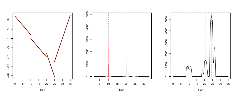
Figure A.2: Left: $X_{i}$ (red) and $f_{i}$ (black). Middle: $W_{k,n}(G)$ with $G=200$ and the local variance estimator $\widehat{\sigma}_{k}$. Right: $W_{k,n}(G)$ with $\sigma$ used in place of $\widehat{\sigma}_{k}$.

Appendix B Practical implementation

B.1 Choice of $H$ for the critical value

Based on Theorem 2.1, we select the critical value $C_{n}(G,\alpha)$ as $C_{n}(G,\alpha)=a_{G}^{-1}\big{(}b_{G}-\log(-\log(1-\alpha)/2)\big{)}$ where $a_{G}=\sqrt{2\log(n/G)}$ and $b_{G}=2\log(n/G)+\log\log(n/G)+\log(H)$. The constant $H$ is found via following simulations.

Randomly generating a sequence of independent random variables $\{X_{i}\}_{i=1}^{n}$ from $\mathcal{N}(0,1)$, we compare the empirical median of $a_{G}W_{n}(G)-2\log(n/G)-\log\log(n/G)$ (setting $\widehat{\tau}_{k}=1$) with the median of $\Gamma_{2}$ to approximate $\log(H)$. Table B.1 lists the approximated values of $\log(H)$ with varying $(n,G)$. Although not reported here, we obtain similar results from the data simulated as $X_{i}\sim\mathcal{N}(a_{0}+a_{1}i,1)$ with varying $(a_{0},a_{1})$. Based on this, in all the numerical experiments, we use $\log(H)\approx 0.7284$. Note that the variation in $\log(H)$ with respect to $(n,G)$ is much smaller than that in $2\log(n/G)$, and hence choice of $\log(H)$ tends not to affect the performance much, see Table B.2.

Table B.1: $\log(H)$ values obtained via simulation with varying $(n,G)$.

$n$	$G$	$\log(H)$	$n$	$G$	$\log(H)$
$10^{5}$	500	0.6375	$10^{6}$	5000	0.7433
$10^{5}$	1000	0.6544	$10^{6}$	10000	0.7284
$10^{5}$	2000	0.6383	$10^{6}$	20000	0.7099

Table B.2: $2\log(n/G)$ values obtained via simulation with varying $(n,G)$.

$n$	$G$	$2\log(n/G)$	$n$	$G$	$2\log(n/G)$
$3500$	100	7.1107	$500$	20	6.4378
$3500$	250	5.2781	$500$	50	4.6052
$3500$	400	4.3381	$500$	80	3.6652

B.2 Efficient computation

The computational complexity of the proposed MOSUM procedure is $O(n)$. To see this, note that the coefficient estimators $\widehat{\boldsymbol{\beta}}^{\pm}(k)$ can be updated as

$$\widehat{\beta}_{1}^{\pm}(k+1)= \,\widehat{\beta}_{1}^{\pm}(k)+B^{\pm}(k),\quad\text{where}\quad A=\sum_{i=1}^{G}\left(i-\frac{G+1}{2}\right)^{2}\Delta t,$$

$$B^{+}(k)= \frac{1}{A}\left(\frac{G-1}{2}X_{k+G+1}-\sum_{i=2}^{G}X_{k+i}+\frac{G-1}{2}X_{k+1}\right)\quad\text{and}$$

$$B^{-}(k)= \frac{1}{A}\left(\frac{G-1}{2}X_{k+1}-\sum_{i=2}^{G}X_{k-G+i}+\frac{G-1}{2}X_{k-G+1}\right),\quad\text{and}$$

$$\widehat{\beta}_{0}^{+}(k+1)- \widehat{\beta}_{0}^{-}(k+1)=\widehat{\beta}_{0}^{+}(k)-\widehat{\beta}_{0}^{-}(k)$$

$$+\frac{1}{G}(X_{k+G+1}-2X_{k+1}+X_{k-G+1})-\left(\frac{G+1}{2}B^{+}(k)+\frac{G-1}{2}B^{-}(k)\right)\Delta t,$$

and the computation of $B^{\pm}(k)$ for all $k$ is of complexity $O(n)$. Similarly, noting that the local variance estimator in (7) can be written as $\widehat{\sigma}_{k}^{2}=(\widehat{\sigma}_{k,+}^{2}+\widehat{\sigma}_{k,-}^{2})/2$ with

$$\widehat{\sigma}_{k,+}^{2} =\frac{1}{G-2}\left(\sum_{i=1}^{G}X_{k+i}^{2}-\frac{1}{G}\left(\sum_{i=1}^{G}X_{k+i}\right)^{2}-(\widehat{\beta}_{1}^{+}(k))^{2}A\Delta t\right)\quad\text{and}$$

$$\widehat{\sigma}_{k,-}^{2} =\frac{1}{G-2}\left(\sum_{i=1}^{G}X_{k-G+i}^{2}-\frac{1}{G}\left(\sum_{i=1}^{G}X_{k-G+i}\right)^{2}-(\widehat{\beta}_{1}^{-}(k))^{2}A\Delta t\right),$$

it can also be updated sequentially.

Appendix C Supplements for the simulation studies

This section complements Section 4 in the main text by providing the complete descriptions of the data generating processes and providing additional simulation results.

C.1 Settings

The piecewise linear signal $f_{i}$ is generated as follows. Throughout, we set $t_{i}=0.01i$.

1. No change point ($J=0$) with $f_{i}=\beta t_{i}+\epsilon_{i}$, $1\leq i\leq n=3500$ where $\beta\sim\mathcal{N}(-1,0.2^{2})$ is randomly drawn for each realization.

2. Piecewise linear and continuous with $J=3$ and

   $$f_{i} =\left\{\begin{array}[]{ll}\beta_{1}(t_{i}-10)+10&(0<i\leq k_{1}=1000)\\ \beta_{2}(t_{i}-10)&(1000<i\leq k_{2}=2000)\\ 10(1+\beta_{2})+\beta_{3}(t_{i}-20)&(2000<i\leq k_{3}=2500)\\ 10(1+\beta_{2})+5\beta_{3}+\beta_{4}(t_{i}-25)&(2500<i\leq n=3500)\end{array}\right.\text{ \ when $n=3500$,}$$ (C.5)

   $$f_{i} =\left\{\begin{array}[]{ll}10\beta_{1}(t_{i}-1)+10&(0<i\leq k_{1}=100)\\ 10\beta_{2}(t_{i}-1)&(100<i\leq k_{2}=200)\\ 10(1+\beta_{2})+\frac{10}{3}\beta_{3}(t_{i}-2)&(200<i\leq k_{3}=350)\\ 10(1+\beta_{2})+5\beta_{3}+\frac{20}{3}\beta_{4}(t_{i}-3.5)&(350<i\leq n=500)\end{array}\right.\text{ \ when $n=500$.}$$ (C.10)

   The vector $\boldsymbol{\beta}=(\beta_{i},\beta_{2},\beta_{3},\beta_{4})^{\top}\sim\mathcal{N}(\boldsymbol{\mu},\sigma_{\beta}^{2}\mathbf{I})$ is randomly drawn for each realization with $\boldsymbol{\mu}=(-1,-1,-2.5,2.5)^{\top}$ and $\sigma_{\beta}=0.2$. Parameters are chosen differently when $n=500$ and $n=3500$ to ensure that $f_{i}$ takes the same values at the three change points regardless of $n$ for given $\boldsymbol{\beta}$. At $i=k_{1}$, the change in the intercept brings a discontinuity to the signal, at $i=k_{2}$, the slope changes as well as there being a discontinuous jump and at $i=k_{3}$, the slope changes while the signal remains continuous. A realization is shown in the top left panel of Figure C.1.

3. Piecewise linear and continuous with $J=3$ and

   $$f_{i} =\left\{\begin{array}[]{ll}\beta_{1}(t_{i}-10)&(0<i\leq k_{1}=1000)\\ \beta_{2}(t_{i}-10)&(1000<i\leq k_{2}=2000)\\ 10\beta_{2}+\beta_{3}(t_{i}-20)&(2000<i\leq k_{3}=2500)\\ 10\beta_{2}+5\beta_{3}+\beta_{4}(t_{i}-25)&(2500<i\leq n=3500)\end{array}\right.\text{ \ when $n=3500$,}$$ (C.15)

   $$f_{i} =\left\{\begin{array}[]{ll}10\beta_{1}(t_{i}-1)&(0<i\leq k_{1}=100)\\ 10\beta_{2}(t_{i}-1)&(100<i\leq k_{2}=200)\\ 10\beta_{2}+\frac{10}{3}\beta_{3}(t_{i}-2)&(200<i\leq k_{3}=350)\\ 10\beta_{2}+5\beta_{3}+\frac{20}{3}\beta_{4}(t_{i}-3.5)&(350<i\leq n=500)\end{array}\right.\text{ \ when $n=500$.}$$ (C.20)

   We generate $(\beta_{1},\beta_{2},\beta_{3},\beta_{4})^{\top}$ as in (M1). The top right panel of Figure C.1 displays a realization.

4. Piecewise linear with frequent changes ($J=6$) and $n=2500$, where

   $$f_{i}=\left\{\begin{array}[]{ll}\beta_{1}(t_{i}-5)&(0<t\leq k_{1}=500)\\ \beta_{2}(t_{i}-5)-10&(500<t\leq k_{2}=800)\\ 3\beta_{2}+\beta_{3}(t_{i}-12)&(800<t\leq k_{3}=1200)\\ 5&(1200<t_{i}\leq k_{4}=1300)\\ 3\beta_{2}+4\beta_{3}+\beta_{4}(t_{i}-12)&(1300<t\leq k_{5}=1700)\\ 3\beta_{2}+4\beta_{3}+5\beta_{4}&(1700<t\leq k_{6}=2100)\\ 3\beta_{2}+4\beta_{3}+5\beta_{4}+\beta_{5}(t_{i}-21)&(2100<t\leq n=2500).\end{array}\right.$$

   Here, $\boldsymbol{\beta}=(\beta_{i},\beta_{2},\beta_{3},\beta_{4},\beta_{5})^{\top}\sim\mathcal{N}(\boldsymbol{\mu},\sigma_{\beta}^{2}\mathbf{I})$ is randomly drawn for each realization with $\boldsymbol{\mu}=(-1,-1,-2.5,2.5,-2.5)^{\top}$ and $\sigma_{\beta}=0.2$. The bottom left panel of Figure C.1 displays one realization from such a model.

5. Piecewise constant with $J=3$ and

   $$f_{i} =\left\{\begin{array}[]{ll}\beta_{1}&(0<i\leq k_{1}=1000)\\ \beta_{2}&(1000<i\leq k_{2}=2000)\\ \beta_{3}&(2000<i\leq k_{3}=2500)\\ \beta_{4}&(2500<i\leq n=3500)\end{array}\right.\text{ \ when $n=3500$,}$$ (C.25)

   $$f_{i} =\left\{\begin{array}[]{ll}3\beta_{1}&(0<i\leq k_{1}=100)\\ 3\beta_{2}&(100<i\leq k_{2}=200)\\ 3\beta_{3}&(200<i\leq k_{3}=350)\\ 3\beta_{4}&(350<i\leq n=500)\end{array}\right.\text{ \ when $n=500$.}$$ (C.30)

   We draw $\boldsymbol{\beta}=(\beta_{1},\beta_{2},\beta_{3},\beta_{4})^{\top}$ from $\mathcal{N}(\boldsymbol{\mu},\sigma_{\beta}^{2}\mathbf{I})$ with $\boldsymbol{\mu}=(-2,2,-5,5)^{\top}$ and $\sigma_{\beta}=0.2$. The bottom right panel of Figure C.1 shows that $f_{i}$ is piecewise constant.

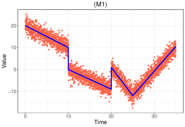
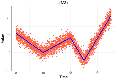
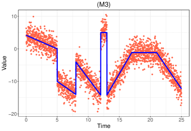
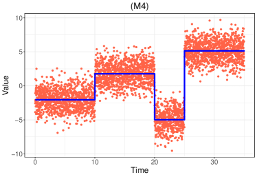
Figure C.1: A realization from (M1), (M2), (M3) and (M4) with Gaussian errors generated as in (E1) with $\sigma=2$. The true signal $f_{i}$ is super-imposed (solid line).

For the generation of $\{\epsilon_{i}\}_{i=1}^{n}$, we consider

1. A sequence of i.i.d. random variables with a normal distribution.

2. A sequence of i.i.d. random variables with a scaled $t_{5}$-distribution.

3. A sequence of i.i.d. random variables with a scaled Laplace distribution whose distribution takes the form with some $s>0$:

   $$f(x;s)=\frac{1}{4s}\exp\left(-\frac{|x|}{2s}\right).$$

4. An AR($1$) process $\epsilon_{i}=\rho\epsilon_{i-1}+\sqrt{1-\rho^{2}}\sigma Z_{i}$ with $\rho\in\{0.3,0.7\}$ and $Z_{i}\sim_{\text{i.i.d.}}\mathcal{N}(0,1)$.

In all above, we vary $\mathsf{Var}(\epsilon_{i})=\sigma^{2}$ with $\sigma\in\{0.5,1,1.5,2\}$.

C.2 Results

Tables C.1–C.7 summarize the simulation results obtained from $1000$ realizations for each setting. As observed in Section 4.2 in the main text, CPOP tends to be much slower with worse performance than the rest of the methods, and thus is included in Tables C.1, C.4 and C.5 only. See Table 4 in the main text for the results under (M0).

Firstly, we consider the results obtained under independence and piecewise linearity, see Tables C.1, C.2, C.4, C.5 and C.6. Overall, the proposed MOSUM procedure estimates the total number and the locations of the change points with high accuracy, and it shows comparable performance as NOT.pwLin or even outperforms latter by a small margin. In particular, MOSUM tends to attain better localization accuracy measured by MAXscore1 and MAXscore2, and the good performance does not depend on the length of the signals, the error generating processes (Gaussianity under (E1) or heavy-tailed under (E2)–(E3)) or the types of changes ((M1), (M2) or (M3)). One exception is when $\sigma=2$ and the signal is short ($n=500$) where we observe slight deterioration in the detection accuracy of MOSUM measured by COUNTscore, see Table C.1. TGUW is generally outperformed by both MOSUM and NOT.pwLin in all scenarios under consideration and in particular, it is prone to return many false positives under non-Gaussianity, as evidenced by large COUNTscore and MAXscore2 (Tables C.2 and C.5).

NOT.pwLinCont and CPOP pre-suppose that the signals are piecewise linear and continuous and as such, in the presence of discontinuities as in (M1), they tend to over-estimate the number of change points by detecting spurious estimators close to the true change points (as evidenced by the small MAXscore1 values), in order to approximate the discontinuous signal by introducing more segments, see Figure C.2 for an example. For piecewise linear and continuous signals under (M2), as expected, NOT.pwLinCont and CPOP perform well under (E1); in particular, the former detects the correct number of change points in almost all realizations, see Table C.4. CPOP has its performance deteriorate greatly in the presence of heavy tails, with larger than $3$ average COUNTscore. The MOSUM procedure performs comparably to NOT.pwLinCont in terms of detection accuracy and even outperforms CPOP in this respect (COUNTscore), but its estimation accuracy is slightly worse than these methods. This may be explained by that our method does not use the extra information that the signal is continuous, i.e. no constraint is imposed when estimating $\widehat{\boldsymbol{\beta}}^{\pm}(k)$. Compared to (M1), we remark that most methods attain worse localization performance under (M2) in the presence of heavy-tailedness noise, see Table C.5.

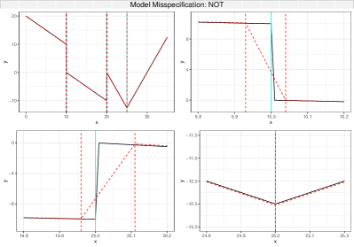
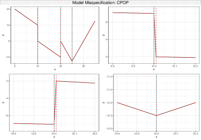
Figure C.2: (M1): Left: NOT.pwLinCont approximates the discontinuous signal $f_{i}$ (top left) around $k_{1}$ and $k_{2}$ by introducing additional change point estimators (top right and bottom left) while estimating the continuous kink at $k_{3}$ well (bottom right). True signal and change point locations are denoted by solid lines, while the estimated signal and change point locations are given by dashed lines. The right panel similarly illustrates the performance of CPOP.

For the case with the serially correlated errors under (E4), see Table C.3 and also Table 2 in the main text and its description.

Under (M4), the signal is piecewise constant with $\alpha_{1,j}=0$ in (1). Hence, we additionally consider NOT.pwConst (‘piecewise constant’) as proposed in Baranowski et al., (2019) besides MOSUM, NOT.pwLin and TGUW, see Table C.7 for the summary of the results. The MOSUM procedure shows comparable or better performance than NOT.pwConst regardless of $n$ when the noise level is small ($\sigma\leq 1.5$), without pre-supposing that the signal is piecewise constant. Its performance is relatively worse when $\sigma=2$ and $n=3500$. Upon close inspection, most inaccuracy stems from that MOSUM occasionally approximates the piecewise constant signal with two constant pieces around $k_{1}$, via a piecewise linear fit with three linear segments, see Figure C.3) for an example of such an instance.

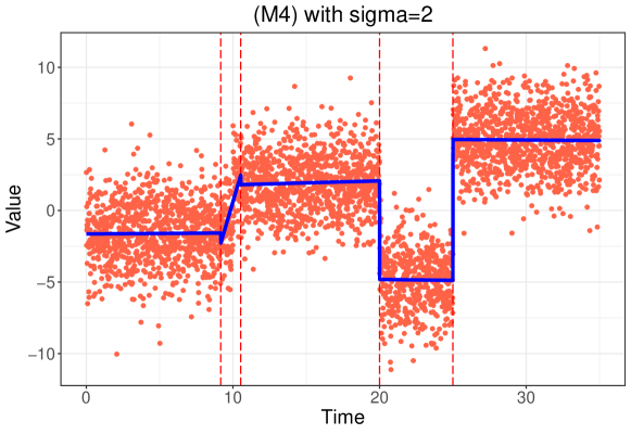
Figure C.3: One realization under (M4) with $n=3500$ with Gaussian errors as in ((E1)) when $\sigma=2$. Vertical broken lines denote the estimated location of changes and the solid line represents the fitted piecewise linear signal based on the change point estimators returned by MOSUM.

Table C.1: (M1): Results from MOSUM, NOT.pwLin, NOT.pwLinCont, CPOP and TGUW when the errors are generated as in (E1) with $\sigma\in\{0.5,1,1.5,2\}$. We report the average and standard error (in parentheses) of the performance metrics over $1000$ realizations.

$(n=500)$	$\sigma$	MOSUM	NOT.pwLin	NOT.pwLinCont	CPOP	TGUW
COUNTscore	$0.5$	0.011 (0.1135)	0.007 (0.0947)	2.165 (1.6169)	2.022 (0.1719)	0.021 (0.1435)
	$1$	0.006 (0.0773)	0.004 (0.0632)	2.419 (2.4152)	2.015 (0.1216)	0.019 (0.1437)
	$1.5$	0.007 (0.0834)	0.007 (0.0834)	2.562 (2.6354)	2.019 (0.1366)	0.039 (0.1988)
	$2$	0.046 (0.2448)	0.004 (0.0632)	2.354 (1.8466)	2.018 (0.1403)	0.095 (0.3034)
MAXscore1	$0.5$	0.019 (0.0139)	0.022 (0.014)	0.016 (0.008)	0.005 (0.0057)	0.028 (0.0217)
	$1$	0.029 (0.0208)	0.039 (0.0237)	0.025 (0.0304)	0.008 (0.0085)	0.046 (0.0344)
	$1.5$	0.04 (0.0292)	0.053 (0.0313)	0.034 (0.0205)	0.012 (0.0099)	0.062 (0.0465)
	$2$	0.052 (0.0421)	0.065 (0.0376)	0.049 (0.0748)	0.017 (0.013)	0.077 (0.0558)
MAXscore2	$0.5$	0.024 (0.0705)	0.025 (0.0555)	0.047 (0.1088)	0.021 (0.1033)	0.029 (0.0288)
	$1$	0.034 (0.0602)	0.041 (0.0379)	0.081 (0.2161)	0.019 (0.078)	0.048 (0.0449)
	$1.5$	0.042 (0.052)	0.057 (0.0678)	0.125 (0.2893)	0.021 (0.0594)	0.065 (0.057)
	$2$	0.057 (0.0562)	0.066 (0.0388)	0.139 (0.2756)	0.026 (0.075)	0.081 (0.0717)
$(n=3500)$	$\sigma$	MOSUM	NOT.pwLin	NOT.pwLinCont	CPOP	TGUW
COUNTscore	$0.5$	0 (0)	0.002 (0.0447)	2.004 (0.1265)	2.003 (0.0547)	0.037 (0.2041)
	$1$	0.001 (0.0316)	0.003 (0.0547)	2.029 (0.3692)	2.007 (0.0947)	0.029 (0.1679)
	$1.5$	0 (0)	0.003 (0.0547)	2.01 (0.1262)	2.004 (0.0894)	0.043 (0.203)
	$2$	0 (0)	0.003 (0.0547)	2.017 (0.1508)	2.004 (0.0632)	0.09 (0.2863)
MAXscore1	$0.5$	0.06 (0.0391)	0.073 (0.0406)	0.033 (0.0134)	0.012 (0.0101)	0.093 (0.068)
	$1$	0.088 (0.0601)	0.123 (0.0653)	0.046 (0.0259)	0.02 (0.0159)	0.152 (0.1142)
	$1.5$	0.105 (0.0724)	0.159 (0.085)	0.062 (0.041)	0.027 (0.0206)	0.203 (0.1475)
	$2$	0.126 (0.0888)	0.193 (0.1057)	0.083 (0.063)	0.037 (0.0278)	0.259 (0.1849)
MAXscore2	$0.5$	0.06 (0.0391)	0.076 (0.0831)	0.079 (0.2573)	0.025 (0.316)	0.119 (0.4068)
	$1$	0.093 (0.1545)	0.131 (0.2561)	0.121 (0.5554)	0.047 (0.4254)	0.158 (0.1386)
	$1.5$	0.105 (0.0724)	0.161 (0.0961)	0.113 (0.4401)	0.041 (0.3216)	0.208 (0.1633)
	$2$	0.126 (0.0888)	0.196 (0.1252)	0.132 (0.3214)	0.048 (0.2331)	0.266 (0.2093)

Table C.2: (M1): Results from MOSUM, NOT.pwLin, NOT.pwLinCont, CPOP and TGUW when $n=3500$ and the errors are generated as in (E2)–(E3) with $\sigma\in\{0.5,1,1.5,2\}$. We report the average and standard error (in parentheses) of the performance metrics over $1000$ realizations.

(E2)	$\sigma$	MOSUM	NOT.pwLin	NOT.pwLinCont	TGUW
COUNTscore	$0.5$	0 (0)	0.016 (0.1783)	2.038 (0.4083)	0.464 (1.1472)
	$1$	0 (0)	0.023 (0.1962)	2.059 (0.4751)	0.472 (1.1741)
	$1.5$	0 (0)	0.02 (0.1888)	2.096 (0.3673)	0.459 (1.1134)
	$2$	0.001 (0.0316)	0.018 (0.1664)	2.14 (0.4434)	0.55 (1.1777)
MAXscore1	$0.5$	0.057 (0.0408)	0.071 (0.0418)	0.033 (0.0136)	0.098 (0.0729)
	$1$	0.083 (0.0574)	0.117 (0.0657)	0.046 (0.0285)	0.172 (0.1219)
	$1.5$	0.106 (0.0757)	0.157 (0.0881)	0.064 (0.0433)	0.235 (0.1644)
	$2$	0.126 (0.0909)	0.196 (0.1109)	0.081 (0.0649)	0.299 (0.2174)
MAXscore2	$0.5$	0.057 (0.0408)	0.129 (0.6975)	0.148 (0.7339)	0.848 (2.1083)
	$1$	0.083 (0.0574)	0.184 (0.776)	0.23 (1.0301)	0.84 (1.9763)
	$1.5$	0.106 (0.0757)	0.22 (0.7302)	0.472 (1.5789)	0.931 (1.9843)
	$2$	0.126 (0.0926)	0.235 (0.5624)	0.538 (1.515)	1.009 (1.9956)
(E3)	$\sigma$	MOSUM	NOT.pwLin	NOT.pwLinCont	TGUW
COUNTscore	$0.5$	0 (0)	0.013 (0.1298)	2.025 (0.3471)	0.603 (1.2966)
	$1$	0 (0)	0.002 (0.0632)	2.017 (0.1917)	0.64 (1.3506)
	$1.5$	0 (0)	0.015 (0.1575)	2.035 (0.3064)	0.672 (1.3814)
	$2$	0 (0)	0.006 (0.0893)	2.039 (0.2399)	0.712 (1.3345)
MAXscore1	$0.5$	0.059 (0.0391)	0.071 (0.0431)	0.032 (0.0134)	0.103 (0.0741)
	$1$	0.083 (0.0582)	0.117 (0.0664)	0.047 (0.0281)	0.176 (0.1259)
	$1.5$	0.108 (0.0776)	0.153 (0.0873)	0.062 (0.0439)	0.237 (0.1632)
	$2$	0.125 (0.0893)	0.187 (0.1047)	0.08 (0.0575)	0.296 (0.2087)
MAXscore2	$0.5$	0.059 (0.0391)	0.091 (0.3739)	0.127 (0.6998)	1.055 (2.3195)
	$1$	0.083 (0.0582)	0.124 (0.2406)	0.11 (0.4325)	1.155 (2.3102)
	$1.5$	0.108 (0.0776)	0.178 (0.4126)	0.15 (0.596)	1.185 (2.2676)
	$2$	0.125 (0.0893)	0.191 (0.1571)	0.224 (0.8226)	1.239 (2.1685)

Table C.3: (M1): Results from MOSUM, MOSUM.dlrv, NOT.pwLin, NOT.pwLinCont, CPOP and TGUW when $n=3500$ and the errors are generated as in (E4) with $\sigma\in\{0.5,1,1.5,2\}$. We report the average and standard error (in parentheses) of the performance metrics over $1000$ realizations.

($\rho=0.3$)	$\sigma$	MOSUM	MOSUM.dlrv	NOT.pwLin	TGUW
COUNTscore	$0.5$	0.036 (0.2162)	0.423 (0.5003)	0.12 (0.4688)	2.366 (2.1947)
	$1$	0.044 (0.2369)	0.492 (0.5237)	0.123 (0.4517)	2.236 (2.1272)
	$1.5$	0.033 (0.1842)	0.693 (0.5649)	0.188 (0.5941)	2.331 (2.1877)
	$2$	0.033 (0.1842)	0.87 (0.5453)	0.17 (0.5342)	2.386 (2.1141)
MAXscore1	$0.5$	0.071 (0.0465)	0.392 (0.3878)	0.087 (0.0532)	0.104 (0.078)
	$1$	0.101 (0.0686)	0.44 (0.3841)	0.142 (0.0795)	0.171 (0.1247)
	$1.5$	0.13 (0.09)	0.552 (0.394)	0.203 (0.125)	0.229 (0.1711)
	$2$	0.159 (0.1151)	0.7 (0.4083)	0.246 (0.1392)	0.287 (0.2122)
MAXscore2	$0.5$	0.205 (0.8384)	0.552 (0.572)	0.366 (1.2819)	3.47 (3.2545)
	$1$	0.241 (0.8473)	0.658 (0.5796)	0.442 (1.3325)	3.403 (3.1662)
	$1.5$	0.25 (0.7988)	0.907 (0.6003)	0.642 (1.5826)	3.566 (3.2606)
	$2$	0.29 (0.8461)	1.156 (0.6117)	0.621 (1.3958)	3.539 (3.1179)
($\rho=0.7$)	$\sigma$	MOSUM	MOSUM.dlrv	NOT.pwLin	TGUW
COUNTscore	$0.5$	8.181 (2.9303)	0.437 (0.5023)	10.966 (7.2253)	123.015 (11.0449)
	$1$	8.16 (2.8497)	0.599 (0.5836)	12.368 (6.1324)	123.405 (10.9049)
	$1.5$	8.097 (2.9567)	0.706 (0.6588)	13.483 (5.4558)	123.218 (10.7549)
	$2$	8.259 (2.9807)	0.987 (0.7399)	13.079 (5.7503)	122.899 (11.013)
MAXscore1	$0.5$	0.092 (0.0687)	0.245 (0.3147)	0.131 (0.1028)	0.088 (0.0737)
	$1$	0.147 (0.1183)	0.43 (0.3839)	0.219 (0.1727)	0.104 (0.095)
	$1.5$	0.206 (0.1662)	0.715 (0.4734)	0.275 (0.2185)	0.112 (0.1083)
	$2$	0.245 (0.1944)	0.979 (0.5241)	0.33 (0.2583)	0.115 (0.1117)
MAXscore2	$0.5$	7.585 (1.5808)	0.588 (0.5667)	6.764 (3.4284)	9.809 (0.1327)
	$1$	7.585 (1.5782)	0.8 (0.6272)	7.784 (2.2462)	9.806 (0.1351)
	$1.5$	7.543 (1.5966)	1.03 (0.8024)	8.302 (1.5665)	9.803 (0.1361)
	$2$	7.577 (1.581)	1.455 (0.9964)	8.151 (1.688)	9.797 (0.1525)

Table C.4: (M2): Results from MOSUM, NOT.pwLin, NOT.pwLinCont, CPOP and TGUW when the errors are generated as in (E1) with $\sigma\in\{0.5,1,1.5,2\}$. We report the average and standard error (in parentheses) of the performance metrics over $1000$ realizations.

($n=500$)	$\sigma$	MOSUM	NOT.pwLin	NOT.pwLinCont	CPOP	TGUW
COUNTscore	$0.5$	0.012 (0.1178)	0.007 (0.0947)	0 (0)	0.028 (0.193)	0.076 (0.2726)
	$1$	0.007 (0.0834)	0.004 (0.0632)	0.001 (0.0316)	0.022 (0.1534)	0.043 (0.2078)
	$1.5$	0.005 (0.0706)	0.014 (0.1258)	0.001 (0.0316)	0.018 (0.1403)	0.047 (0.221)
	$2$	0.003 (0.0547)	0.006 (0.0773)	0.003 (0.0547)	0.02 (0.1601)	0.04 (0.2108)
MAXscore1	$0.5$	0.034 (0.0147)	0.041 (0.0164)	0.011 (0.0052)	0.013 (0.007)	0.055 (0.026)
	$1$	0.053 (0.0237)	0.07 (0.0261)	0.02 (0.0097)	0.021 (0.013)	0.09 (0.0411)
	$1.5$	0.073 (0.0344)	0.096 (0.0372)	0.028 (0.0158)	0.029 (0.018)	0.124 (0.0579)
	$2$	0.089 (0.0389)	0.12 (0.0447)	0.038 (0.0213)	0.038 (0.0225)	0.152 (0.0674)
MAXscore2	$0.5$	0.04 (0.0695)	0.043 (0.0342)	0.011 (0.0052)	0.025 (0.1117)	0.061 (0.0551)
	$1$	0.057 (0.0597)	0.071 (0.035)	0.02 (0.01)	0.028 (0.0848)	0.094 (0.0531)
	$1.5$	0.075 (0.0537)	0.099 (0.0485)	0.028 (0.0195)	0.035 (0.0796)	0.128 (0.0682)
	$2$	0.09 (0.0435)	0.122 (0.0512)	0.039 (0.0271)	0.046 (0.0898)	0.157 (0.0826)
($n=3500$)	$\sigma$	MOSUM	NOT.pwLin	NOT.pwLinCont	CPOP	TGUW
COUNTscore	$0.5$	0.002 (0.0447)	0.004 (0.0632)	0 (0)	0.007 (0.0834)	0.093 (0.3073)
	$1$	0 (0)	0 (0)	0 (0)	0.003 (0.0547)	0.069 (0.2652)
	$1.5$	0 (0)	0.001 (0.0316)	0 (0)	0.006 (0.0773)	0.073 (0.2641)
	$2$	0 (0)	0.003 (0.0547)	0 (0)	0.005 (0.0706)	0.065 (0.2466)
MAXscore1	$0.5$	0.122 (0.0552)	0.16 (0.0616)	0.023 (0.0121)	0.028 (0.0207)	0.229 (0.1176)
	$1$	0.186 (0.0883)	0.262 (0.1016)	0.047 (0.0253)	0.05 (0.0261)	0.372 (0.1817)
	$1.5$	0.254 (0.1327)	0.359 (0.1431)	0.073 (0.0409)	0.076 (0.0528)	0.506 (0.2401)
	$2$	0.32 (0.1639)	0.44 (0.1728)	0.099 (0.0565)	0.1 (0.0634)	0.623 (0.2983)
MAXscore2	$0.5$	0.130 (0.2598)	0.168 (0.2147)	0.023 (0.0121)	0.046 (0.4038)	0.246 (0.1674)
	$1$	0.186 (0.0883)	0.262 (0.1016)	0.047 (0.0253)	0.054 (0.0969)	0.393 (0.2488)
	$1.5$	0.254 (0.1327)	0.359 (0.1431)	0.073 (0.0409)	0.079 (0.1024)	0.531 (0.309)
	$2$	0.32 (0.1639)	0.442 (0.193)	0.099 (0.0565)	0.109 (0.2848)	0.648 (0.368)

Table C.5: (M2): Results from MOSUM, NOT.pwLin, NOT.pwLinCont, CPOP and TGUW when $n=3500$ and the errors are generated as in (E2)–(E3) with $\sigma\in\{0.5,1,1.5,2\}$. We report the average and standard error (in parentheses) of the performance metrics over $1000$ realizations.

(E2)	$\sigma$	MOSUM	NOT.pwLin	NOT.pwLinCont	CPOP	TGUW
COUNTscore	$0.5$	0 (0)	0.005 (0.0836)	0 (0)	5.903 (4.2374)	0.596 (1.2459)
	$1$	0.003 (0.0547)	0.019 (0.1633)	0.004 (0.0632)	5.989 (4.1427)	0.659 (1.237)
	$1.5$	0.001 (0.0316)	0.018 (0.1473)	0.005 (0.0948)	6.402 (4.2131)	0.847 (1.3869)
	$2$	0.007 (0.0834)	0.023 (0.2203)	0.006 (0.0773)	6.051 (4.1983)	0.744 (1.276)
MAXscore1	$0.5$	0.178 (0.103)	0.252 (0.1352)	0.045 (0.0332)	0.09 (0.1164)	0.414 (0.2632)
	$1$	0.336 (0.5639)	0.454 (0.5608)	0.123 (0.5478)	0.204 (0.3175)	0.751 (0.6129)
	$1.5$	0.418 (0.3909)	0.577 (0.308)	0.145 (0.1045)	0.298 (0.3109)	1 (0.6024)
	$2$	0.53 (0.7981)	0.714 (0.6252)	0.225 (0.5635)	0.421 (0.4754)	1.238 (0.8628)
MAXscore2	$0.5$	0.178 (0.103)	0.274 (0.4542)	0.045 (0.0332)	4.518 (3.2269)	1.168 (2.0277)
	$1$	0.306 (0.1857)	0.482 (0.728)	0.102 (0.311)	4.634 (3.2025)	1.501 (1.9696)
	$1.5$	0.408 (0.244)	0.642 (0.7988)	0.159 (0.3044)	4.884 (3.1902)	1.965 (2.1865)
	$2$	0.471 (0.295)	0.731 (0.6933)	0.201 (0.2448)	4.53 (3.196)	2.024 (2.034)
(E3)	$\sigma$	MOSUM	NOT.pwLin	NOT.pwLinCont	CPOP	TGUW
COUNTscore	$0.5$	0 (0)	0.003 (0.0547)	0 (0)	3.532 (3.4054)	0.815 (1.401)
	$1$	0.002 (0.0447)	0.016 (0.1542)	0.002 (0.0447)	3.606 (3.3289)	0.866 (1.443)
	$1.5$	0.001 (0.0316)	0.008 (0.0891)	0 (0)	3.53 (3.2711)	0.855 (1.4177)
	$2$	0.005 (0.0706)	0.013 (0.1444)	0.002 (0.0632)	3.8 (3.1957)	0.841 (1.337)
MAXscore1	$0.5$	0.189 (0.1125)	0.251 (0.1279)	0.046 (0.033)	0.079 (0.084)	0.425 (0.264)
	$1$	0.314 (0.4752)	0.424 (0.4657)	0.111 (0.4489)	0.168 (0.3693)	0.747 (0.5885)
	$1.5$	0.39 (0.3798)	0.584 (0.3116)	0.151 (0.1275)	0.274 (0.297)	0.943 (0.5587)
	$2$	0.528 (0.7272)	0.703 (0.3865)	0.195 (0.1642)	0.36 (0.3768)	1.204 (0.8215)
MAXscore2	$0.5$	0.189 (0.1125)	0.27 (0.443)	0.046 (0.033)	3.17 (3.3651)	1.471 (2.2634)
	$1$	0.294 (0.182)	0.433 (0.4659)	0.092 (0.0677)	3.221 (3.3163)	1.761 (2.2033)
	$1.5$	0.381 (0.2392)	0.615 (0.6003)	0.151 (0.1275)	3.117 (3.2616)	1.875 (2.0448)
	$2$	0.48 (0.3102)	0.709 (0.4006)	0.198 (0.2067)	3.332 (3.2156)	2.137 (2.0815)

Table C.6: (M3): Results from MOSUM, NOT.pwLin and TGUW when the errors are generated as in (E1)–(E3) with $\sigma\in\{0.5,1,1.5,2\}$. We report the average and standard error (in parentheses) of the performance metrics over $1000$ realizations.

(E1)	$\sigma$	MOSUM	NOT.pwLin	TGUW
COUNTscore	$0.5$	0 (0)	0.001 (0.0316)	0.083 (0.3003)
	$1$	0 (0)	0.003 (0.0547)	0.196 (0.5328)
	$1.5$	0.008 (0.0891)	0.001 (0.0316)	0.274 (0.6598)
	$2$	0.031 (0.1734)	0.003 (0.0547)	0.37 (0.8086)
MAXscore1	$0.5$	0.111 (0.0592)	0.144 (0.0574)	0.198 (0.1066)
	$1$	0.182 (0.0943)	0.244 (0.0965)	0.319 (0.1676)
	$1.5$	0.272 (0.3497)	0.331 (0.1353)	0.455 (0.2347)
	$2$	0.313 (0.3155)	0.412 (0.1764)	0.564 (0.2768)
MAXscore2	$0.5$	0.111 (0.0592)	0.145 (0.058)	0.217 (0.1597)
	$1$	0.182 (0.0943)	0.248 (0.1671)	0.433 (0.4911)
	$1.5$	0.243 (0.131)	0.331 (0.1353)	0.604 (0.5761)
	$2$	0.293 (0.1698)	0.414 (0.1789)	0.731 (0.6109)
(E2)	$\sigma$	MOSUM	NOT.pwLin	TGUW
COUNTscore	$0.5$	0 (0)	0.024 (0.1716)	0.383 (0.8793)
	$1$	0 (0)	0.025 (0.1685)	0.485 (0.9406)
	$1.5$	0.013 (0.1133)	0.031 (0.2147)	0.472 (0.9198)
	$2$	0.035 (0.1892)	0.03 (0.1927)	0.505 (0.9321)
MAXscore1	$0.5$	0.116 (0.0636)	0.147 (0.0623)	0.215 (0.1071)
	$1$	0.18 (0.0917)	0.239 (0.1029)	0.384 (0.1921)
	$1.5$	0.281 (0.4169)	0.328 (0.1402)	0.539 (0.2566)
	$2$	0.303 (0.2415)	0.402 (0.1803)	0.664 (0.3307)
MAXscore2	$0.5$	0.116 (0.0636)	0.157 (0.1742)	0.412 (0.6519)
	$1$	0.18 (0.0917)	0.248 (0.1997)	0.607 (0.6723)
	$1.5$	0.242 (0.1665)	0.342 (0.229)	0.768 (0.7023)
	$2$	0.296 (0.1805)	0.442 (0.395)	0.902 (0.737)
(E3)	$\sigma$	MOSUM	NOT.pwLin	TGUW
COUNTscore	$0.5$	0 (0)	0.01 (0.1262)	0.504 (1.0673)
	$1$	0 (0)	0.007 (0.0947)	0.518 (1.0221)
	$1.5$	0.01 (0.0995)	0.015 (0.1442)	0.498 (0.9607)
	$2$	0.058 (0.2544)	0.009 (0.1045)	0.615 (1.1189)
MAXscore1	$0.5$	0.112 (0.0605)	0.15 (0.0613)	0.222 (0.1148)
	$1$	0.177 (0.0976)	0.244 (0.0999)	0.392 (0.1863)
	$1.5$	0.279 (0.3972)	0.333 (0.1368)	0.526 (0.2588)
	$2$	0.311 (0.2349)	0.412 (0.184)	0.676 (0.3179)
MAXscore2	$0.5$	0.112 (0.0605)	0.156 (0.1239)	0.504 (0.8012)
	$1$	0.177 (0.0976)	0.251 (0.203)	0.646 (0.7245)
	$1.5$	0.24 (0.1269)	0.337 (0.1483)	0.756 (0.7051)
	$2$	0.308 (0.1983)	0.421 (0.2496)	0.915 (0.7361)

Table C.7: (M4): Results from MOSUM, NOT.pwLin, NOT.pwConst and TGUW when the errors are generated as in (E1) with $\sigma\in\{0.5,1,1.5,2\}$. We report the average and standard error (in parentheses) of the performance metrics over $1000$ realizations.

$(n=500)$	$\sigma$	MOSUM	NOT.pwLin	NOT.pwConst	TGUW
COUNTscore	$0.5$	0.002 (0.0447)	0.001 (0.0316)	0.039 (0.2086)	0.007 (0.1377)
	$1$	0.005 (0.0706)	0.005 (0.0706)	0.034 (0.1868)	0.003 (0.0707)
	$1.5$	0.005 (0.0706)	0.001 (0.0316)	0.039 (0.227)	0.007 (0.1047)
	$2$	0.01 (0.0995)	0.005 (0.0706)	0.054 (0.2778)	0.024 (0.1657)
MAXscore1	$0.5$	0 (0)	0 (0)	0 (0)	0 (0)
	$1$	0 (0)	0 (0)	0 (0)	0 (0)
	$1.5$	0 (0)	0 (0)	0 (0)	0 (0.0018)
	$2$	0.001 (0.0107)	0 (0.0033)	0 (0.001)	0.001 (0.0048)
MAXscore2	$0.5$	0.001 (0.0288)	0.001 (0.0256)	0.012 (0.0876)	0.001 (0.0238)
	$1$	0.002 (0.0345)	0.001 (0.0204)	0.012 (0.0915)	0.001 (0.0178)
	$1.5$	0.002 (0.0285)	0 (0.0073)	0.015 (0.1092)	0.003 (0.0511)
	$2$	0.004 (0.0465)	0.003 (0.0504)	0.022 (0.1319)	0.005 (0.0563)
$(n=3500)$	$\sigma$	MOSUM	NOT.pwLin	NOT.pwConst	TGUW
COUNTscore	$0.5$	0 (0)	0.003 (0.0547)	0.006 (0.0773)	0.005 (0.0706)
	$1$	0 (0)	0.001 (0.0316)	0.008 (0.0891)	0.073 (0.2603)
	$1.5$	0.018 (0.133)	0.005 (0.0706)	0.011 (0.1135)	0.173 (0.3889)
	$2$	0.162 (0.382)	0 (0)	0.019 (0.1366)	0.263 (0.4879)
MAXscore1	$0.5$	0 (0)	0 (0)	0 (0)	0 (0.0018)
	$1$	0.001 (0.0026)	0.001 (0.0026)	0.001 (0.0026)	0.006 (0.0131)
	$1.5$	0.013 (0.0741)	0.003 (0.0064)	0.003 (0.0064)	0.021 (0.0335)
	$2$	0.121 (0.2746)	0.007 (0.0108)	0.007 (0.011)	0.049 (0.0761)
MAXscore2	$0.5$	0 (0)	0.014 (0.3351)	0.012 (0.299)	0.001 (0.0142)
	$1$	0.001 (0.0026)	0.001 (0.0048)	0.035 (0.4835)	0.008 (0.0185)
	$1.5$	0.017 (0.0971)	0.024 (0.4353)	0.037 (0.498)	0.028 (0.0523)
	$2$	0.155 (0.3468)	0.007 (0.0108)	0.062 (0.5403)	0.068 (0.1884)

C.3 Empirical size control

We additionally conduct numerical experiments to examine the size control of the proposed MOSUM-based test. For this, we adopt the null model (M0) in Section C.1 with Gaussian errors generated as in (E1) with varying variance to generate $1000$ realizations. On each realization, we compute the test statistics $W_{n}(G)$ and examine whether it exceeds a threshold. Here, we compare two approaches to get the threshold: (i) theoretically motivated critical value $C_{n}(G,\alpha)=a_{G}^{-1}\big{(}b_{G}-\log(-\log(1-\alpha)/2)\big{)}$ with $\alpha=0.05$ and $\log(H)=0.7284$ as suggested in Section 3.3, and (ii) the empirical critical value obtained as the sample $(1-\alpha)$-quantile of the simulated values of $W_{n}(G)$ for given $n$ and $G$. We note that while (i) does not require the knowledge of the data generating process, (ii) does. Table C.8 shows that as expected, the approach (ii) results in the empirical size close to the significance level $\alpha=0.05$, whereas (i) tends to be more conservative. With both approaches, using the proposed multiscale extension with bandwidths $\mathcal{G}=\{50,100,150,250,400,650\}$, we also produce an estimator $\widehat{J}_{n}$ of the number of change points ($J=0$), the results from which are summarized in Table C.9. From this, we conclude that using either asymptotic or empirical critical values leads to satisfactory size control and estimation consistency under $\mathcal{H}_{0}:\,J=0$, but the former approach is more preferable as it depends only on $n$ and $G$ and does not require the prior knowledge of the data generating process or heavy computation.

Table C.8: Empirical sizes when using (i) asymptotic and (ii) empirical critical values for varying $G$ and $\sigma$.

	$G=50$	$G=100$	$G=150$	$G=250$	$G=400$	$G=650$
Asymptotic critical value
$\sigma=0.5$	0.035	0.015	0.013	0.012	0.008	0.002
$\sigma=1$	0.038	0.020	0.012	0.010	0.010	0.008
$\sigma=1.5$	0.019	0.020	0.014	0.008	0.005	0.003
$\sigma=2$	0.033	0.022	0.013	0.015	0.005	0.002
Empirical critical value
$\sigma=0.5$	0.054	0.053	0.045	0.041	0.039	0.053
$\sigma=1$	0.050	0.060	0.056	0.057	0.054	0.059
$\sigma=1.5$	0.040	0.051	0.043	0.036	0.037	0.052
$\sigma=2$	0.051	0.052	0.048	0.053	0.034	0.056

Table C.9: Accuracy in estimating the number of change points when using (i) asymptotic and (ii) empirical critical values. We report the average and standard error (in parentheses) of COUNTscore over $1000$ realizations.

	Asymptotic	Empirical
$\sigma=0.5$	0 (0)	0 (0)
$\sigma=1$	0 (0)	0 (0)
$\sigma=1.5$	0.001 (0.0316)	0 (0)
$\sigma=2$	0 (0)	0 (0)

Appendix D Proofs

This section gives the proofs for the theorems. We define $\mathbf{x}_{i,k}=(1,(i-k)/G)^{\top}$ and let

$$\mathbf{C}_{G,+}=\begin{bmatrix}G&\frac{G+1}{2}\\ \frac{G+1}{2}&\frac{(G+1)(2G+1)}{6G}\end{bmatrix}\quad\text{and}\quad\mathbf{C}_{G,-}=\begin{bmatrix}G&-\frac{G-1}{2}\\ -\frac{G-1}{2}&\frac{(G-1)(2G-1)}{6G}\end{bmatrix}.$$

Further, we define

$$\mathbf{C}_{+}=\begin{bmatrix}1&\frac{1}{2}\\ \frac{1}{2}&\frac{1}{3}\end{bmatrix},\quad\mathbf{D}_{G,+}=\begin{bmatrix}0&\frac{1}{2G}\\ \frac{1}{2G}&\frac{1}{2G}+\frac{1}{6G^{2}}\end{bmatrix},\quad\text{and}$$ (D.1)

$$\mathbf{C}_{-}=\begin{bmatrix}1&-\frac{1}{2}\\ -\frac{1}{2}&\frac{1}{3}\end{bmatrix},\quad\mathbf{D}_{G,-}=\begin{bmatrix}0&\frac{1}{2G}\\ \frac{1}{2G}&-\frac{1}{2G}+\frac{1}{6G^{2}}\end{bmatrix},$$ (D.2)

so that $G^{-1}\mathbf{C}_{G,+}=\mathbf{C}_{+}+\mathbf{D}_{G,+}$ and $G^{-1}\mathbf{C}_{G,-}=\mathbf{C}_{-}+\mathbf{D}_{G,-}$. Throughout, for a matrix $\mathbf{A}\in\mathbb{R}^{p\times q}$, we denote by $\|\mathbf{A}\|_{r}$ the matrix norms induced by vector $r$-norms for a given $r$. We denote by $\mathbf{0}$ and $\mathbf{I}$ the vector of zeros and the identity matrix, respectively, whose dimensions are determined in the context. For a finite-dimensional matrix $\mathbf{A}$, we write $\mathbf{A}=O(G^{-1})$ to denote that all its elements are bounded as $O(G^{-1})$.

D.1 Preliminary lemmas

Lemma D.1.

$$G\mathbf{C}_{G,+}^{-1}=\mathbf{C}_{+}^{-1}+\frac{1}{G-1}\begin{bmatrix}6&-6\\ -6&\frac{12}{G+1}\end{bmatrix}\quad\text{and}\quad G\mathbf{C}_{G,-}^{-1}=\mathbf{C}_{-}^{-1}+\frac{1}{G+1}\begin{bmatrix}-6&-6\\ -6&\frac{12}{G-1}\end{bmatrix}.$$

Lemma D.2.

Assume that (A1)–(A2) hold and let $\widetilde{W}(t)=G^{-1/2}W(Gt)$. Then,

$$\sup_{1\leq t\leq\frac{n}{G}-1}\left|G^{-1/2}\sum_{i=\lfloor tG\rfloor+1}^{\lfloor tG\rfloor+G}\mathbf{x}_{i,\lfloor tG\rfloor}\epsilon_{i}-\tau\int_{t}^{t+1}\begin{bmatrix}1\\ (s-t)\end{bmatrix}\mathop{}\!\mathrm{d}\widetilde{W}(s)\right|=o_{P}\left(\frac{1}{\sqrt{\log(n/G)}}\right),$$ (D.3)

$$\sup_{1\leq t\leq\frac{n}{G}-1}\left|G^{-1/2}\sum_{i=\lfloor tG\rfloor-G+1}^{\lfloor tG\rfloor}\mathbf{x}_{i,\lfloor tG\rfloor}\epsilon_{i}-\tau\int_{t-1}^{t}\begin{bmatrix}1\\ (s-t)\end{bmatrix}\mathop{}\!\mathrm{d}\widetilde{W}(s)\right|=o_{P}\left(\frac{1}{\sqrt{\log(n/G)}}\right).$$ (D.4)

Proof.

Assumption (A1) implies that

$$\max_{G\leq k\leq n-G}\left|\sum_{i=k+1}^{k+G}\epsilon_{i}-\tau\left(W(k+G)-W(k)\right)\right|=O\left(n^{\frac{1}{2+\nu}}\right)\quad\text{ a.s.}$$

It also implies that, for $\alpha=1,2,\ldots$, (Csörgő and Horváth,, 1997, page 237),

$$\frac{1}{n^{\alpha}}\left|\sum_{i=1}^{n}i^{\alpha}\epsilon_{i}-\tau\int_{0}^{n}s^{\alpha}\mathop{}\!\mathrm{d}W(s)\right|=O\left(n^{\frac{1}{2+\nu}}\right)\quad\text{ {a.s.}}\quad\text{where}$$

$$\left\{\int_{0}^{t}s^{\alpha}\mathop{}\!\mathrm{d}W(s),\,0\leq t<\infty\right\}\overset{d}{\equiv}\left\{W\left(\frac{1}{2\alpha+1}t^{2\alpha+1}\right),~{}0\leq t<\infty\right\}.$$

Thus we have

$$\max_{G\leq k\leq n-G}\left|\sum_{i=k+1}^{k+G}\frac{i-k}{G}\epsilon_{i}-\frac{\tau}{G}\int_{k}^{k+G}(s-k)\mathop{}\!\mathrm{d}W(s)\right|=O\left(\frac{n^{1+\frac{1}{2+\nu}}}{G}\right)\quad\text{a.s.}$$

As $W(t)$ satisfies

$$\sup_{1\leq t\leq N-1}\sup_{0\leq s<1}|W(t+s)-W(t)|=O\left(\sqrt{\log(N)}\right)\quad\text{a.s.,}$$

and by Theorem 1.2.1 of Csörgő and Révész, (1979), the Gaussian process $Y(t)=\int_{0}^{t}s\mathop{}\!\mathrm{d}W(s)$ satisfies

$$\sup_{1\leq t\leq N-1}\sup_{0\leq s<1}|Y(t+s)-Y(t)|=O\left(N\sqrt{\log(N)}\right)\quad\text{a.s.,}$$

we obtain

$$\sup_{1\leq t\leq\frac{n}{G}-1}\left|\int_{\lfloor tG\rfloor}^{\lfloor tG\rfloor+G}\mathop{}\!\mathrm{d}W(s)-\int_{tG}^{(t+1)G}\mathop{}\!\mathrm{d}W(s)\right|$$

$$=\sup_{1\leq t\leq\frac{n}{G}-1}\left|\left(W\big{(}\lfloor(t+1)G\rfloor\big{)}-W\big{(}(t+1)G\big{)}\right)-\left(W\big{(}\lfloor tG\rfloor\big{)}-W\big{(}tG\big{)}\right)\right|=O\left(\sqrt{\log(n)}\right)\text{ \ a.s.,}$$

$$\sup_{1\leq t\leq\frac{n}{G}-1}\left|\int_{\lfloor tG\rfloor}^{\lfloor tG\rfloor+G}(s-\lfloor tG\rfloor)\mathop{}\!\mathrm{d}W(s)-\int_{tG}^{(t+1)G}(s-tG)\mathop{}\!\mathrm{d}W(s)\right|$$

$$\leq\sup_{1\leq t\leq\frac{n}{G}-1}\bigg{\{}\Big{|}Y\big{(}tG\big{)}-Y\big{(}\lfloor tG\rfloor\big{)}\Big{|}+\Big{|}Y\big{(}(t+1)G\big{)}-Y\big{(}\lfloor(t+1)G\rfloor\big{)}\Big{|}$$

$$\quad+\lfloor tG\rfloor\Big{|}W\big{(}tG\big{)}-W\big{(}\lfloor tG\rfloor\big{)}\Big{|}+\lfloor tG\rfloor\Big{|}W\big{(}(t+1)G\big{)}-W\big{(}\lfloor(t+1)G\rfloor\big{)}\Big{|}$$

$$\quad+\sqrt{G}\big{(}tG-\lfloor tG\rfloor\big{)}\Big{|}\widetilde{W}\big{(}t+1\big{)}-\widetilde{W}\big{(}t\big{)}\Big{|}\bigg{\}}=O\left(n\sqrt{\log(n)}\right)\text{ \ a.s.}$$

Then for $k=\lfloor tG\rfloor$, we have

$$\sup_{1\leq t\leq\frac{n}{G}-1}\left|\sum_{i=\lfloor tG\rfloor+1}^{\lfloor tG\rfloor+G}\mathbf{x}_{i,k}\epsilon_{i}-\tau\int_{tG}^{(t+1)G}\begin{bmatrix}1\\ (s-tG)/G\end{bmatrix}\mathop{}\!\mathrm{d}W(s)\right|=O\left(\frac{n^{1+\frac{1}{2+\nu}}}{G}+\frac{n{\sqrt{\log(n)}}}{G}\right)\text{ \ a.s.}$$

Together with (3), we have (D.3) and (D.4) is similarly derived. ∎

Lemma D.3.

Assume that (A1)–(A2) hold.

$$\frac{1}{\sqrt{G}}\max_{G\leq k\leq n-G}\left|\sum_{i=k+1}^{k+G}\mathbf{x}_{i,k}\epsilon_{i}\right| =O_{P}\left(\sqrt{\log(n/G)}\right),$$ (D.5)

$$\frac{1}{\sqrt{G}}\max_{G\leq k\leq n-G}\left|\sum_{i=k-G+1}^{k}\mathbf{x}_{i,k}\epsilon_{i}\right| =O_{P}\left(\sqrt{\log(n/G)}\right).$$ (D.6)

Proof.

By Lemma D.2,

$$\max_{G\leq k\leq n-G}\ \left|\sum_{i=k+1}^{k+G}\mathbf{x}_{i,k}\epsilon_{i}\right| =\sup_{1\leq t\leq n/G-1}\left|\tau\int_{t}^{t+1}\begin{bmatrix}1\\ (s-t)\end{bmatrix}\mathop{}\!\mathrm{d}\widetilde{W}(s)\right|+o_{P}\left(\frac{1}{\sqrt{\log(n/G)}}\right)$$

and as for $\widetilde{Y}(t)=\int_{0}^{t}s\mathop{}\!\mathrm{d}\widetilde{W}(s)$, elements of

$$\int_{t}^{t+1}\begin{bmatrix}1\\ (s-t)\end{bmatrix}\mathop{}\!\mathrm{d}\widetilde{W}(s)=\begin{bmatrix}\widetilde{W}(t+1)-\widetilde{W}(t)\\ \widetilde{Y}(t+1)-\widetilde{Y}(t)-t\big{(}\widetilde{W}(t+1)-\widetilde{W}(t)\big{)}\end{bmatrix}$$

are stationary Gaussian processes with zero means and constant variances. More specifically, $\mathsf{Var}(\widetilde{W}(t+1)-\widetilde{W}(t))=1$ and

$$\mathsf{Var}\left(\widetilde{Y}(t+1)-\widetilde{Y}(t)\right) =\mathsf{Var}\left(\int_{t}^{t+1}s\mathop{}\!\mathrm{d}\widetilde{W}(s)\right)=t^{2}+t+\frac{1}{3},\quad\text{and}$$

$$\mathsf{Cov}\left(\widetilde{Y}(t+1)-\widetilde{Y}(t),\widetilde{W}(t+1)-\widetilde{W}(t)\right) =\mathsf{Cov}\left(\int_{t}^{t+1}s\mathop{}\!\mathrm{d}\widetilde{W}(s),\int_{t}^{t+1}\mathop{}\!\mathrm{d}\widetilde{W}(s)\right)=t+\frac{1}{2}$$

such that the variance of the second element is $1/3$. From this, (D.5) follows and (D.6) can similarly be shown. ∎

D.2 Proof of Theorem 2.1

For the proof of Theorem 2.1, we first establish that $\sqrt{G}/\tau\cdot\boldsymbol{\Sigma}^{-1/2}(\widehat{\boldsymbol{\beta}}^{+}(k)-\widehat{\boldsymbol{\beta}}^{-}(k))$ is well-approximated by a stationary bivariate Gaussian process $\mathbf{Z}(t)=(Z_{0}(t),Z_{1}(t))^{\top}$ with a known covariance structure, where $k=\lfloor tG\rfloor$ (Proposition D.4). A Wald-type MOSUM statistic has been considered in Kirch and Reckruehm, (2022) for detecting changes in linear regression where such Gaussian approximation plays a similar role in deriving the asymptotic null distribution. However, their results are not applicable to our setting due to the presence of the trend under (1), which leads to $Z_{0}(t)$ and $Z_{1}(t)$ with non-zero cross-(auto)covariance. This makes the investigation into the asymptotic null distribution more challenging and introduces the undetermined constant $\log(H)$. We carefully address this issue and derive the asymptotic null distribution of $\sup_{1\leq t\leq n/G-1}\|\mathbf{Z}(t)\|$ (Proposition D.5).

Proposition D.4.

Assume that (A1)–(A2) hold and that $G$ fulfils (3). Then under $\mathcal{H}_{0}$,

$$\sup_{1\leq t\leq n/G-1}\left|\left\|\frac{\sqrt{G}}{\tau}\boldsymbol{\Sigma}^{-1/2}\left(\widehat{\boldsymbol{\beta}}^{+}(\lfloor tG\rfloor)-\widehat{\boldsymbol{\beta}}^{-}(\lfloor tG\rfloor)\right)\right\|-\left\|\begin{bmatrix}Z_{0}(t)\\ Z_{1}(t)\end{bmatrix}\right\|\right|=o_{P}\left(\frac{1}{\sqrt{\log(n/G)}}\right),$$

where $\mathbf{Z}(t)=(Z_{0}(t),Z_{1}(t))^{\top}$ is a stationary, bivariate Gaussian process with $\mathsf{E}(\mathbf{Z}(t))=\mathbf{0}$ and $\mathsf{Cov}(\mathbf{Z}(t))=\mathbf{I}$ at each $t$, and

$$\mathsf{Cov}(Z_{0}(t),Z_{0}(t+h)) =\left\{\begin{array}[]{ll}1-\frac{9}{2}|h|+3|h|^{2}+\frac{3}{4}|h|^{3}&(|h|<1)\\ -1+\frac{7}{2}|h|-3|h|^{2}+\frac{3}{4}|h|^{3}&(1\leq|h|<2)\\ 0&(\text{otherwise}),\end{array}\right.$$ (D.10)

$$\mathsf{Cov}(Z_{1}(t),Z_{1}(t+h)) =\left\{\begin{array}[]{ll}1-\frac{3}{2}|h|-3|h|^{2}+3|h|^{3}&(|h|<1)\\ -1-\frac{3}{2}|h|+3|h|^{2}-|h|^{3}&(1\leq|h|<2)\\ 0&(\text{otherwise}),\end{array}\right.\quad\text{and}$$ (D.14)

$$\mathsf{Cov}(Z_{0}(t),Z_{1}(t+h)) =\left\{\begin{array}[]{ll}-\frac{3\sqrt{3}}{2}h+\frac{9\sqrt{3}}{4}h^{2}-\frac{\sqrt{3}}{2}h^{3}&(0\leq h<1)\\ \frac{3\sqrt{3}}{2}h-\frac{7\sqrt{3}}{4}h^{2}+\frac{\sqrt{3}}{2}h^{3}&(1\leq h<2)\\ -\frac{3\sqrt{3}}{2}h-\frac{9\sqrt{3}}{4}h^{2}-\frac{\sqrt{3}}{2}h^{3}&(-1<h<0)\\ \frac{3\sqrt{3}}{2}h+\frac{7\sqrt{3}}{4}h^{2}+\frac{\sqrt{3}}{2}h^{3}&(-2<h\leq-1)\\ 0&(\text{otherwise}).\end{array}\right.$$ (D.20)

Proposition D.5.

Let $M(T)=\sup_{1\leq t\leq T}\sqrt{Z_{0}^{2}(t)+Z_{1}^{2}(t)}$ with $Z_{0}(t)$ and $Z_{1}(t)$ defined in Proposition D.4. Then, there exists a constant $H>0$ such that we have

$$a_{T}M(T)-b_{T}\xrightarrow[n\to\infty]{d}\Gamma_{2},\quad\text{where}$$

$$a_{T}=\sqrt{2\log(T)},\quad b_{T}=2\log(T)+\log\log(T)+\log(H)$$

and $\Gamma_{2}$ is as in Theorem 2.1.

Proof of Theorem 2.1.

Combining Propositions D.4 and D.5, we have

$$a_{G}\max_{G\leq k\leq n-G}W^{*}_{k,n}(G)-b_{G}\xrightarrow[n\to\infty]{d}\Gamma_{2},\quad\text{with}\quad W^{*}_{k,n}(G)=\ \frac{\sqrt{G}}{\tau}\left\|\boldsymbol{\Sigma}^{-1/2}\left(\widehat{\boldsymbol{\beta}}^{+}(k)-\widehat{\boldsymbol{\beta}}^{-}(k)\right)\right\|.$$ (D.21)

Noting that $W_{k,n}(G)=\tau W_{k,n}^{*}(G)/\widehat{\tau}_{k}$, from (B1), we have

$$\max_{G\leq k\leq n-G}\left|W_{k,n}(G)-W^{*}_{k,n}(G)\right|\leq\frac{\max_{k}|\widehat{\tau}_{k}-\tau|}{\sqrt{\tau^{2}-\max_{k}|\widehat{\tau}_{k}^{2}-\tau^{2}|}}\max_{k}W_{k,n}(G)=o_{P}\left(\frac{1}{\sqrt{\log(n/G)}}\right).$$

∎

D.2.1 Proof of Proposition D.4

Since $J_{n}=0$, we have

$$\widehat{\boldsymbol{\beta}}^{+}(k)-\widehat{\boldsymbol{\beta}}^{-}(k)=\mathbf{C}_{G,+}^{-1}\sum_{i=k+1}^{k+G}\mathbf{x}_{i,k}\epsilon_{i}-\mathbf{C}_{G,-}^{-1}\sum_{i=k-G+1}^{k}\mathbf{x}_{i,k}\epsilon_{i}.$$

Then by Lemmas D.1, D.2 and D.3, for $k=\lfloor tG\rfloor$,

$$\frac{\sqrt{G}}{\tau}\left(\widehat{\boldsymbol{\beta}}^{+}(k)-\widehat{\boldsymbol{\beta}}^{-}(k)\right) =\frac{1}{\tau\sqrt{G}}\left\{\left(\mathbf{C}_{+}^{-1}+O(G^{-1})\right)\sum_{i=k+1}^{k+G}\mathbf{x}_{i,k}\epsilon_{i}-\left(\mathbf{C}_{-}^{-1}+O(G^{-1})\right)\sum_{i=k-G+1}^{k}\mathbf{x}_{i,k}\epsilon_{i}\right\}$$

$$=\mathbf{C}_{+}^{-1}\int_{t}^{t+1}\begin{bmatrix}1\\ s-t\end{bmatrix}\mathop{}\!\mathrm{d}\widetilde{W}(s)-\mathbf{C}_{-}^{-1}\int_{t-1}^{t}\begin{bmatrix}1\\ s-t\end{bmatrix}\mathop{}\!\mathrm{d}\widetilde{W}(s)+R_{k}$$

with $\max_{G\leq k\leq n-G}\|R_{k}\|_{2}=O_{P}(\sqrt{\log(n/G)}/G)=o_{P}(1/\sqrt{\log(n/G)})$. Recalling that $\widetilde{Y}(t)=\int_{0}^{t}s\mathop{}\!\mathrm{d}\widetilde{W}(s)$, we have

$$\boldsymbol{\Sigma}^{-1/2}\left\{\mathbf{C}_{+}^{-1}\int_{t}^{t+1}\begin{bmatrix}1\\ s-t\end{bmatrix}\mathop{}\!\mathrm{d}\widetilde{W}(s)-\mathbf{C}_{-}^{-1}\int_{t-1}^{t}\begin{bmatrix}1\\ s-t\end{bmatrix}\mathop{}\!\mathrm{d}\widetilde{W}(s)\right\}$$

$$= \,\boldsymbol{\Sigma}^{-1/2}\left\{\begin{bmatrix}4&-6\\ -6&12\end{bmatrix}\begin{bmatrix}\widetilde{W}(t+1)-\widetilde{W}(t)\\ \widetilde{Y}(t+1)-\widetilde{Y}(t)-t\big{(}\widetilde{W}(t+1)-\widetilde{W}(t)\big{)}\end{bmatrix}\right.$$

$$\left.\qquad\qquad\qquad-\begin{bmatrix}4&6\\ 6&12\end{bmatrix}\begin{bmatrix}\widetilde{W}(t)-\widetilde{W}(t-1)\\ \widetilde{Y}(t)-\widetilde{Y}(t-1)-t\big{(}\widetilde{W}(t)-\widetilde{W}(t-1)\big{)}\end{bmatrix}\right\}$$

$$= \,\boldsymbol{\Sigma}^{-1/2}\left\{\begin{bmatrix}4+6t&-6\\ -(6+12t)&12\end{bmatrix}\begin{bmatrix}\widetilde{W}(t+1)-\widetilde{W}(t)\\ \widetilde{Y}(t+1)-\widetilde{Y}(t)\end{bmatrix}-\begin{bmatrix}4-6t&6\\ 6-12t&6\end{bmatrix}\begin{bmatrix}\widetilde{W}(t)-\widetilde{W}(t-1)\\ \widetilde{Y}(t)-\widetilde{Y}(t-1)\end{bmatrix}\right\}$$

$$=: \,\mathbf{Z}(t)=\begin{bmatrix}Z_{0}(t)\\ Z_{1}(t)\end{bmatrix},$$

it holds that

$$\sup_{1\leq t\leq\frac{n}{G}-1}\left\|\frac{\sqrt{G}}{\tau}\boldsymbol{\Sigma}^{-1/2}\left(\widehat{\boldsymbol{\beta}}^{+}(\lfloor tG\rfloor)-\widehat{\boldsymbol{\beta}}^{-}(\lfloor tG\rfloor)\right)-\begin{bmatrix}Z_{0}(t)\\ Z_{1}(t)\end{bmatrix}\right\|=o_{P}\left(\frac{1}{\sqrt{\log(n/G)}}\right),$$

which gives the assertion. What remains is to establish (D.10)–(D.20), which are shown in the following Lemmas D.6–D.7.

Lemma D.6.

Let

$$\Omega(t,h):=\mathsf{Cov}\left(\begin{bmatrix}\widetilde{W}(t+1+h)-\widetilde{W}(t+h)\\ \widetilde{Y}(t+1+h)-\widetilde{Y}(t+h)\end{bmatrix},\begin{bmatrix}\widetilde{W}(t+1)-\widetilde{W}(t)\\ \widetilde{Y}(t+1)-\widetilde{Y}(t)\end{bmatrix}\right).$$

Then

$$\Omega(t,h)=\left\{\begin{array}[]{ll}\begin{bmatrix}1-h&(1-h)t+\frac{1-h^{2}}{2}\\ (1-h)t+\frac{1-h^{2}}{2}&(1-h)t^{2}+(1-h^{2})t+\frac{1-h^{3}}{3}\end{bmatrix}&(0\leq h<1)\\ \begin{bmatrix}1+h&(1+h)t+\frac{(1+h)^{2}}{2}\\ (1+h)t+\frac{(1+h)^{2}}{2}&(1+h)t^{2}+(1+h)^{2}t+\frac{(1+h)^{3}}{3}\end{bmatrix}&(-1<h<0)\\ \mathbf{0}&(|h|\geq 1).\end{array}\right.$$

Proof.

Let $f(t)$ and $g(t)$ be continuous functions. For $t,s>0$, simple calculations give

$$\mathsf{Cov}\left(\int_{0}^{t+1}f(u)\mathop{}\!\mathrm{d}\widetilde{W}(u)-\int_{0}^{t}f(u)\mathop{}\!\mathrm{d}\widetilde{W}(u),\int_{0}^{s+1}g(u)\mathop{}\!\mathrm{d}\widetilde{W}(u)-\int_{0}^{s}g(u)\mathop{}\!\mathrm{d}\widetilde{W}(u)\right)$$

$$=\int_{\min(\max(t,s),\min(t,s)+1)}^{\min(t,s)+1}f(u)g(u)\mathop{}\!\mathrm{d}u.$$

Now denote $\Omega(t,h)=\begin{bmatrix}\Omega_{11}(t,h)&\Omega_{12}(t,h)\\ \Omega_{21}(t,h)&\Omega_{22}(t,h)\end{bmatrix}$. Then,

$$\Omega_{11}(t,h) =\left\{\begin{array}[]{ll}\int_{t+h}^{t+1}\mathop{}\!\mathrm{d}u&(0\leq h<1)\\ \int_{t}^{t+1+h}\mathop{}\!\mathrm{d}u&(-1<h<0)\\ 0&(|h|\geq 1)\end{array}\right.=\left\{\begin{array}[]{ll}1-h&(0\leq h<1)\\ 1+h&(-1<h<0)\\ 0&(|h|\geq 1),\end{array}\right.$$

$$\Omega_{12}(t,h) =\left\{\begin{array}[]{ll}\int_{t+h}^{t+1}u\mathop{}\!\mathrm{d}u&(0\leq h<1)\\ \int_{t}^{t+1+h}u\mathop{}\!\mathrm{d}u&(-1<h<0)\\ 0&(|h|\geq 1)\end{array}\right.=\left\{\begin{array}[]{ll}(1-h)t+\frac{1-h^{2}}{2}&(0\leq h<1)\\ (1+h)t+\frac{(1+h)^{2}}{2}&(-1<h<0)\\ 0&(|h|\geq 1),\end{array}\right.$$

$$\Omega_{21}(t,h) =\left\{\begin{array}[]{ll}\int_{t+h}^{t+1}u\mathop{}\!\mathrm{d}u&(0\leq h<1)\\ \int_{t}^{t+1+h}u\mathop{}\!\mathrm{d}u&(-1<h<0)\\ 0&(|h|\geq 1)\end{array}\right.=\left\{\begin{array}[]{ll}(1-h)t+\frac{1-h^{2}}{2}&(0\leq h<1)\\ (1+h)t+\frac{(1+h)^{2}}{2}&(-1<h<0)\\ 0&(|h|\geq 1),\end{array}\right.$$

$$\Omega_{22}(t,h) =\left\{\begin{array}[]{ll}\int_{t+h}^{t+1}u^{2}\mathop{}\!\mathrm{d}u&(0\leq h<1)\\ \int_{t}^{t+1+h}u^{2}\mathop{}\!\mathrm{d}u&(-1<h<0)\\ 0&(|h|\geq 1)\end{array}\right.=\left\{\begin{array}[]{ll}(1-h)t^{2}+(1-h^{2})t+\frac{1-h^{3}}{3}&(0\leq h<1)\\ (1+h)t^{2}+(1+h)^{2}t+\frac{(1+h)^{3}}{3}&(-1<h<0)\\ 0&(|h|\geq 1).\end{array}\right.$$

∎

Lemma D.7.

The Gaussian process $\mathbf{Z}(t)$ satisfies (D.10)–(D.20).

Proof.

For notational simplicity, we define

$$\mathbf{A}(t)=\boldsymbol{\Sigma}^{-1/2}\begin{bmatrix}4+6t&-6\\ -(6+12t)&12\end{bmatrix},~{}\mathbf{B}(t)=\boldsymbol{\Sigma}^{-1/2}\begin{bmatrix}4-6t&6\\ 6-12t&12\end{bmatrix}\text{ and }\mathbf{V}(t)=\begin{bmatrix}\tilde{W}(t+1)-\tilde{W}(t)\\ \tilde{Y}(t+1)-\tilde{Y}(t)\end{bmatrix}.$$

Then $\mathbf{Z}(t)=\mathbf{A}(t)\mathbf{V}(t)-\mathbf{B}(t)\mathbf{V}(t-1)$ and by Lemma D.6, we have $\mathsf{Cov}(\mathbf{V}(t+h),\mathbf{V}(t))=\Omega(t,h)$. Therefore,

$$\mathsf{Cov}\left(\begin{bmatrix}Z_{0}(t+h)\\ Z_{1}(t+h)\end{bmatrix},\begin{bmatrix}Z_{0}(t)\\ Z_{1}(t)\end{bmatrix}\right)=\begin{bmatrix}\mathsf{Cov}(Z_{0}(t+h),Z_{0}(t))&\mathsf{Cov}(Z_{0}(t+h),Z_{1}(t))\\ \mathsf{Cov}(Z_{1}(t+h),Z_{0}(t))&\mathsf{Cov}(Z_{1}(t+h),Z_{1}(t))\end{bmatrix}$$

$$=\mathsf{Cov}\big{(}\mathbf{A}(t+h)\mathbf{V}(t+h)-\mathbf{B}(t+h)\mathbf{V}(t-1+h),\mathbf{A}(t)\mathbf{V}(t)-\mathbf{B}(t)\mathbf{V}(t-1)\big{)}$$

$$=\mathbf{A}(t+h)\Omega(t,h)\mathbf{A}(t)^{\top}-\mathbf{B}(t+h)\Omega(t,-1+h)\mathbf{A}(t)^{\top}$$

$$-\mathbf{A}(t+h)\Omega(t-1,1+h)\mathbf{B}(t)^{\top}+\mathbf{B}(t+h)\Omega(t-1,h)\mathbf{B}(t)^{\top}.$$ (D.22)

Case 1: $0\leq h<1$.

Then as $-1\leq-1+h<0$ and $1\leq 1+h<2$,

$$\Omega(t,-1+h)=\begin{bmatrix}h&ht+\frac{h^{2}}{2}\\ ht+\frac{h^{2}}{2}&ht^{2}+h^{2}t+\frac{h^{3}}{3}\end{bmatrix},~{}\Omega(t-1,1+h)=\begin{bmatrix}0&0\\ 0&0\end{bmatrix},$$

and hence

$$\mathsf{Cov}\left(\begin{bmatrix}Z_{0}(t+h)\\ Z_{1}(t+h)\end{bmatrix},\begin{bmatrix}Z_{0}(t)\\ Z_{1}(t)\end{bmatrix}\right)=\begin{bmatrix}\frac{6h^{3}+24h^{2}-36h+8}{8}&\frac{6h(2h^{2}-9h+6)}{8\sqrt{3}}\\ \frac{-6h(2h^{2}-9h+6)}{8\sqrt{3}}&\frac{12(6h^{3}-6h^{2}-3h+2)}{24}\end{bmatrix}.$$ (D.23)

Case 2: $1\leq h<2$.

Then as $0\leq-1+h<1$ and $1+h\geq 2$,

$$\Omega(t,-1+h)=\begin{bmatrix}2-h&(2-h)t+h-\frac{h^{2}}{2}\\ (2-h)t+h-\frac{h^{2}}{2}&(2-h)t^{2}-(2h-h^{2})t+\frac{2-h^{3}}{3}-h+h^{2}\end{bmatrix}$$

and $\Omega(t,h)$, $\Omega(t-1,1+h)$, $\Omega(t-1,h)$ are all the zero matrices. Therefore

$$\mathsf{Cov}\left(\begin{bmatrix}Z_{0}(t+h)\\ Z_{1}(t+h)\end{bmatrix},\begin{bmatrix}Z_{0}(t)\\ Z_{1}(t)\end{bmatrix}\right)=\begin{bmatrix}\frac{6h^{3}-24h^{2}+28h-8}{8}&\frac{-2h(6h^{2}-21h+18)}{8\sqrt{3}}\\ \frac{2h(6h^{2}-21h+18)}{8\sqrt{3}}&\frac{-12(2h^{3}-6h^{2}+3h+2)}{24}\end{bmatrix}.$$ (D.24)

Case 3: $-1\leq h<0$.

Then as $0\leq 1+h<1$ and $-1+h<1$, $\Omega(t,-1+h)$ is a zero matrix and

$$\Omega(t-1,1+h)=\begin{bmatrix}-h&-ht-\frac{h^{2}}{2}\\ -ht-\frac{h^{2}}{2}&-ht^{2}-h^{2}t-\frac{h^{3}}{3}\end{bmatrix}.$$

Therefore we get

$$\mathsf{Cov}\left(\begin{bmatrix}Z_{0}(t+h)\\ Z_{1}(t+h)\end{bmatrix},\begin{bmatrix}Z_{0}(t)\\ Z_{1}(t)\end{bmatrix}\right)=\begin{bmatrix}\frac{-6h^{3}+24h^{2}+36h+8}{8}&\frac{6h(2h^{2}+9h+6)}{8\sqrt{3}}\\ \frac{-6h(2h^{2}+9h+6)}{8\sqrt{3}}&\frac{12(-6h^{3}-6h^{2}+3h+2)}{24}\end{bmatrix}.$$ (D.25)

Case 4: $-2\leq h<-1$.

Then as $-1+h<-2$ and $-1\leq 1+h<0$,

$$\Omega(t-1,1+h)=\begin{bmatrix}2+h&(2+h)t+h+\frac{h^{2}}{2}\\ (2+h)t+h+\frac{h^{2}}{2}&(2+h)t^{2}+(2h+h^{2})t+\frac{2+h^{3}}{3}+h+h^{2}\end{bmatrix}$$

and $\Omega(t,h)$, $\Omega(t-1,1+h)$, $\Omega(t,-1+h)$ are all the zero matrices. Therefore

$$\mathsf{Cov}\left(\begin{bmatrix}Z_{0}(t+h)\\ Z_{1}(t+h)\end{bmatrix},\begin{bmatrix}Z_{0}(t)\\ Z_{1}(t)\end{bmatrix}\right)=\begin{bmatrix}\frac{-6h^{3}-24h^{2}-28h-8}{8}&\frac{-2h(6h^{2}+21h+18)}{8\sqrt{3}}\\ \frac{2h(6h^{2}+21h+18)}{8\sqrt{3}}&\frac{12(2h^{3}+6h^{2}+3h-2)}{24}\end{bmatrix}.$$ (D.26)

Case 5: $|h|\geq 2$.

In this case, $\Omega(t,h)$, $\Omega(t-1,1+h)$, $\Omega(t,-1+h)$, $\Omega(t-1,h)$ are all zero matrices. Hence

$$\mathsf{Cov}\left(\begin{bmatrix}Z_{0}(t+h)\\ Z_{1}(t+h)\end{bmatrix},\begin{bmatrix}Z_{0}(t)\\ Z_{1}(t)\end{bmatrix}\right)=\begin{bmatrix}0&0\\ 0&0\end{bmatrix}.$$ (D.27)

Combining (D.23)–(D.27) with (D.22) gives (D.10)–(D.20). ∎

D.2.2 Proof of Proposition D.5

Theorem 10 of Albin, (1990) gives that their Conditions A($\{0\}$), B, C${}^{0}(\{0\})$, D(0), D^′ and Equation (2.15) imply

$$\lim_{u\to\infty}\Pr\left(w(u)^{-1}\left(\sup_{t\in[0,T(u)]}\|\mathbf{Z}(t)\|-u\right)\leq x\right)=\exp\big{(}-(1-F(x))^{1-c}\big{)}$$ (D.28)

where $T(u)\sim\frac{q(u)}{H(1-G(u))}$ as $u\to\infty$ (hereafter, $a(u)\sim b(u)$ means $a(u)/b(u)\to 1$ as $u\to\infty$), $q(u)=u^{-2}$, $G(u)$ is a marginal distribution function of $\|\mathbf{Z}(t)\|$, and $w(u)$, $F$, $c\in[0,1]$ are defined in the conditions. We first show that all the required conditions hold with $w(u)=u^{-1}$, $F(x)=1-e^{-x}$ and $c=0$, and then apply the arguments adopted in Steinebach and Eastwood, (1996) to complete the proof.

Condition A$(\{0\})$ is implied by Equations (2.1), (2.12) and (2.13) of Albin, (1990) by Theorem 3 therein. As marginal density $g$ of $\|\mathbf{Z}(t)\|$ is $g(x)=xe^{-x^{2}/2}$, $G$ satisfies their (2.1) and (2.12) with $w(u)=u^{-1}$ and $F(x)=1-e^{-x}$ (also refer to Theorem 9 of Albin, (1990)). Next, assume that Condition B has been shown. Then Condition C${}^{0}(\{0\})$ is implied by Condition A$(\{0\})$, B, and C by Theorem 2 (c) of Albin, (1990), and as Condition C is achieved by proving (2.23) by Theorem 6 of Albin, (1990), proving (2.23) with Condition B gives Condition C${}^{0}(\{0\})$. Condition D(0) and D^′ follow immediately as auto- and cross-covariance functions of $\mathbf{Z}(t)$ are locally supported. Finally, we can show that (2.15) of Albin, (1990) holds from that

$$\frac{q(u+x/u)}{q(u)}=\frac{u}{u+x/u}\to 1\text{ as }u\to\infty.$$

Therefore, combining all above, it remains to verify Equation (2.13), Condition B, and Equation (2.23).

Equation (2.13):

Let $\omega(t)=\|\mathbf{Z}(t)\|$. We show that there exist a random sequence $\{\eta_{a,x}(k)\}_{k=1}^{\infty}$ and such that, for all $a>0$ and all $N$,

$$\left(u\left(\omega(aq)-u\right),\ldots,u\left(\omega(aqN)-u\right)\left|\right.u\left(\omega(0)-u\right)=x\right)\xrightarrow[u\to\infty]{d}(\eta_{a,x}(1),\ldots,\eta_{a,x}(N))$$

for almost all $x>0$, where $q=q(u)=u^{-2}$. Let $r_{i}(h)=\mathsf{Cov}(Z_{i}(t),Z_{i}(t+h))$ for $i=0,1$ and

$$\boldsymbol{\Sigma}(qt)=\mathsf{Cov}(\mathbf{Z}(qt),\mathbf{Z}(0))=\begin{bmatrix}1-\frac{9}{2}qt&-\frac{3\sqrt{3}}{2}qt\\ \frac{3\sqrt{3}}{2}qt&1-\frac{3}{2}qt\end{bmatrix}+o(qt)=:\begin{bmatrix}1-C_{0}qt&-C_{01}qt\\ -C_{10}qt&1-C_{1}qt\end{bmatrix}+o(qt).$$

Also define $\mathbf{Z}^{u}(t)=u(\mathbf{Z}(qt)-\boldsymbol{\Sigma}(qt)\mathbf{Z}(0))$ and $\Delta_{i}(t)=u\big{(}u+\frac{x}{u}\big{)}(1-r_{i}(qt))$, and denote by $\kappa^{2}$ the one-dimensional Hausdorff measure over $\mathbb{R}^{2}$. If we write $u(\omega(0)-u)=x$ as $\mathbf{Z}(0)=\left(u+\frac{x}{u}\right){\mathbf{x}}$ with some ${\mathbf{x}}=(x_{0},x_{1})$ satisfying $\|\mathbf{x}\|=1$, we have $Z_{i}(qt)=Z_{i}(0)+o(1)$ as $u\to\infty$ (and hence $q\to 0$) and

$$\omega(aqk)-\omega(0) =\frac{\sum_{i=0}^{1}(Z_{i}^{2}(aqk)-Z_{i}^{2}(0))}{\omega(aqk)+\omega(0)}=\frac{\sum_{i=0}^{1}(Z_{i}(aqk)-Z_{i}(0))(2Z_{i}(0)+o(1))}{2\omega(0)+o(1)}$$

$$=\frac{\sum_{i=0}^{1}\left(u+\frac{x}{u}\right)x_{i}\big{(}Z_{i}(aqk)-Z_{i}(0)\big{)}+o(1)}{u+\frac{x}{u}+o(1)}=\sum_{i=0}^{1}x_{i}\big{(}Z_{i}(aqk)-Z_{i}(0)\big{)}+o(u^{-1}).$$

With $\cdot$ denoting the inner product, we have

$$\Pr\left(\left.\bigcap_{k=1}^{N}\left\{u\big{(}\omega(aqk)-u\big{)}\leq z_{k}\right\}\right|u\big{(}\omega(0)-u\big{)}=x\right)$$

$$= \int_{\|{\mathbf{x}}\|=1}\Pr\left(\left.\bigcap_{k=1}^{N}\left\{u\big{(}\omega(aqk)-\omega(0)\big{)}+x\leq z_{k}\right\}\right|\mathbf{Z}(0)=\left(u+\frac{x}{u}\right){\mathbf{x}}\right)\frac{(2\pi)^{-1}\left(u+\frac{x}{u}\right)}{g\left(u+\frac{x}{u}\right)\exp\left(\frac{1}{2}\left(u+\frac{x}{u}\right)^{2}\right)}\mathop{}\!\mathrm{d}\kappa^{2}({\mathbf{x}})$$

$$= \frac{1}{2\pi}\int_{\|{\mathbf{x}}\|=1}\Pr\left(\left.\bigcap_{k=1}^{N}\left\{\sum_{i=0}^{1}ux_{i}\big{(}Z_{i}(aqk)-Z_{i}(0)\big{)}+x+o(1)\leq z_{k}\right\}\right|\mathbf{Z}(0)=\left(u+\frac{x}{u}\right){\mathbf{x}}\right)\mathop{}\!\mathrm{d}\kappa^{2}({\mathbf{x}})$$

$$= \frac{1}{2\pi}\int_{\|{\mathbf{x}}\|=1}\Pr\left(\left.\bigcap_{k=1}^{N}\left\{{\mathbf{x}}\cdot\mathbf{Z}^{u}(aqk)-u{\mathbf{x}}\cdot(\mathbf{I}-\boldsymbol{\Sigma}(aqk))\mathbf{Z}(0)+x+o(1)\leq z_{k}\right\}\right|\mathbf{Z}(0)=\left(u+\frac{x}{u}\right){\mathbf{x}}\right)\mathop{}\!\mathrm{d}\kappa^{2}({\mathbf{x}})$$

$$= \frac{1}{2\pi}\int_{\|{\mathbf{x}}\|=1}\Pr\left(\left.\bigcap_{k=1}^{N}\left\{{\mathbf{x}}\cdot\mathbf{Z}^{u}(aqk)-(u^{2}+x){\mathbf{x}}\cdot(\mathbf{I}-\boldsymbol{\Sigma}(aqk))\mathbf{x}+x+o(1)\leq z_{k}\right\}\right|\mathbf{Z}(0)=\left(u+\frac{x}{u}\right){\mathbf{x}}\right)\mathop{}\!\mathrm{d}\kappa^{2}({\mathbf{x}})$$

$$= \frac{1}{2\pi}\int_{\|{\mathbf{x}}\|=1}\Pr\left(\bigcap_{k=1}^{N}\left\{{\mathbf{x}}\cdot\mathbf{Z}^{u}(aqk)-(u^{2}+x)\sum_{i=0}^{1}C_{i}aqkx_{i}^{2}+x+o(1)\leq z_{k}\right\}\right)\mathop{}\!\mathrm{d}\kappa^{2}({\mathbf{x}})$$

from the independence between $(\mathbf{Z}^{u}(t_{k}))_{k=1}^{N}$ and $\mathbf{Z}(0)$. Noting that

$$\mathsf{Cov}(\mathbf{Z}^{u}(t),\mathbf{Z}^{u}(s)) =u^{2}\mathsf{Cov}\big{(}\mathbf{Z}(qt)-\boldsymbol{\Sigma}(qt)\mathbf{Z}(0),\mathbf{Z}(qs)-\boldsymbol{\Sigma}(qs)\mathbf{Z}(0)\big{)}$$

$$=u^{2}(\boldsymbol{\Sigma}(q(t-s))-\boldsymbol{\Sigma}(qt)\boldsymbol{\Sigma}(qs)^{\top})=(t+s-|t-s|)\begin{bmatrix}\frac{9}{2}&0\\ 0&\frac{3}{2}\end{bmatrix}+o(1),$$

the normally distributed $(\mathbf{Z}^{u}(ak))_{k=1}^{N}$ converges to multivariate normal random vectors $\big{(}\boldsymbol{\zeta}(t_{k})\big{)}_{k=1}^{N}$ with $\boldsymbol{\zeta}(t_{k})=(\zeta_{0}(t_{k}),\zeta_{1}(t_{k}))^{\top}$, where $\zeta_{0}(t)$ and $\zeta_{1}(t)$ are independent zero-mean Gaussian processes with $\mathsf{Cov}(\zeta_{i}(s),\zeta_{i}(t))=C_{i}(t+s-|t-s|)$. Finally, noting that $(u^{2}+x)C_{i}aqk\to C_{i}ak$, we have the finite dimensional distributions of $\left\{\big{(}u(\omega(qt)-u)|u(\omega(0)-u)=x\big{)}\right\}_{t>0}$ converge weakly to those of $\{\eta(t)\}_{t>0}$, where

$$\Pr\left(\bigcap_{k=1}^{N}\left\{\eta(aqk)\leq z_{k}\right\}\right)=\frac{1}{2\pi}\int_{|\mathbf{x}|=1}\Pr\left(\bigcap_{k=1}^{N}\left\{\mathbf{x}\cdot{\boldsymbol{\zeta}}(ak)-\sum_{i=1}^{m}C_{i}x_{i}^{2}ak+x\leq z_{k}\right\}\right)\mathop{}\!\mathrm{d}\kappa^{2}(\mathbf{x}).$$

Condition B:

We show that

$$\displaystyle\limsup_{u\to\infty}\sum_{k=N}^{[h/(aq)]}\Pr\big{(}\omega(aqk)>u|\omega(0)>u\big{)}\to 0$$

when $N\to\infty$, for all fixed $a>0$ and some $h>0$. Let $\boldsymbol{\Sigma}(t)$ have singular values $\lambda_{1}(t)\geq\lambda_{2}(t)>0$. Choose constants $A,B,\epsilon>0$ such that $At\leq 1-\lambda_{i}(t)\leq Bt$ for $0<t\leq\epsilon$, and let $R=\lambda_{1}(qt)$, $r=\lambda_{2}(qt)$ and $\mathbf{Z}_{\bar{r}}(qt)=\boldsymbol{\Sigma}(qt)\mathbf{Z}(0)$. Then by the triangle inequality, for $\omega(qt)>\omega(0)>u$,

$$u(1-R)<\omega(qt)-R\omega(0)\leq\omega(qt)-\|\mathbf{Z}_{\bar{r}}(qt)\|\leq\|\mathbf{Z}(qt)-\mathbf{Z}_{\bar{r}}(qt)\|.$$

Also note that for any vector $\mathbf{v}$, we have $\mathbf{v}^{\top}(\mathbf{I}-\boldsymbol{\Sigma}(qt)\boldsymbol{\Sigma}(qt)^{\top})\mathbf{v}{\leq(1-r^{2})\mathbf{v}^{\top}\mathbf{v}}$. Hence using symmetry and Boole’s inequality,

$$\Pr\big{(}\omega(qt)>u,\,\omega(0)>u\big{)}=2\Pr\big{(}\omega(qt)>\omega(0)>u\big{)}$$

$$\leq 2\Pr\big{(}\omega(0)>u,\|\mathbf{Z}(qt)-\mathbf{Z}_{\bar{r}}(qt)\|>u(1-R)\big{)}$$

$$=2\Pr\big{(}\omega(0)>u\big{)}\Pr\big{(}\|\mathbf{Z}(qt)-\mathbf{Z}_{\bar{r}}(qt)\|>u(1-R)\,\big{|}\,\omega(0)>u\big{)}$$

$$\leq 2(1-G(u))\Pr\left(\sqrt{\chi^{2}_{2}}>\frac{(1-R)u}{\sqrt{1-r^{2}}}\right)\leq 2(1-G(u))\sum_{i=0}^{1}\Pr\left(|Z_{i}|>{\frac{(1-R)u}{\sqrt{2(1-r^{2})}}}\right)$$

$$\leq 8(1-G(u))\left(1-\Phi\left(\frac{(1-R)u}{\sqrt{2(1-r^{2})}}\right)\right)$$

where with a slight abuse of notation, we denote by $\chi^{2}_{2}$ a random variable following the chi-squared distribution, and $Z_{i},\,i=0,1$, denote independent standard normal random variables. Then,

$$\frac{1}{1-G(u)}\Pr\big{(}\omega(qt)>u,\omega(0)>u\big{)}\leq 8\big{(}1-\Phi(A(4B)^{-1/2}t^{1/2})\big{)}\text{ for }0<qt\leq\epsilon,$$

$$\frac{1}{1-G(u)}\Pr\big{(}\omega(qt)>u,\omega(0)>u\big{)}\leq 8\big{(}1-\Phi(\lambda 2^{-1/2}u)\big{)}\text{ for }\epsilon<qt\leq h,$$

where $\lambda=1-\sup_{s\in(\epsilon,h]}\max(\lambda_{1}(s),\lambda_{2}(s))$. From this, Condition B follows since

$$\sum_{k=N}^{\left\lfloor\frac{h}{aq}\right\rfloor}\Pr\big{(}\omega(aqk)>u\big{|}\omega(0)>u\big{)}$$

$$\leq 8\left\{\sum_{k=N}^{\left\lfloor\frac{\epsilon}{aq}\right\rfloor}\left(1-\Phi\left(\frac{A}{\sqrt{4B}}(ak)^{1/2}\right)\right)+\left(\left\lfloor\frac{h}{aq}\right\rfloor-\left\lfloor\frac{\epsilon}{aq}\right\rfloor\right)\left(1-\Phi\left(\frac{\lambda}{\sqrt{2}}u\right)\right)\right\}$$

$$\leq 8\left(\int_{N}^{\infty}\frac{\frac{1}{\sqrt{2\pi}}\exp\left(-\frac{A^{2}}{8B}(ax)\right)}{\frac{A}{\sqrt{4B}}(ax)^{1/2}}\mathop{}\!\mathrm{d}x+\left(\left\lfloor\frac{h}{aq}\right\rfloor-\left\lfloor\frac{\epsilon}{aq}\right\rfloor\right)\frac{\frac{1}{\sqrt{2\pi}}\exp\left(-\frac{\lambda^{2}}{4}u^{2}\right)}{\frac{\lambda}{\sqrt{2}}u}\right)\xrightarrow[N\to\infty]{}0.$$

Equation (2.23):

We show that there exist constants $\lambda_{0}$, $\rho$, $e$, $C$, $\delta_{0}>0$, $u_{0}>0$ and $d>1$ such that

$$\Pr\big{(}\omega(qt)-\omega(0)>\lambda w(u),\omega(0)\leq u+\delta_{0}w(u)\big{|}\omega(qt)>u\big{)}\leq Ct^{d}\lambda^{-e}$$

for all $0<t^{\rho}<\lambda<\lambda_{0}$ and $u>u_{0}$.

Set $\delta\in(0,1)$ and the constants $B$, $\epsilon>0$ such that $\lambda_{i}(t)>\frac{1}{2}$ and $1-\lambda_{i}(t)\leq Bt$ for $0<t\leq\epsilon$, for $i=1,2$, and let $\lambda_{0}=\min(\epsilon^{1/2},1/(8B))$. Further, let $u_{0}=1$ and $\mathbf{Z}_{\bar{r}}^{\prime}(qt)=\boldsymbol{\Sigma}(qt)^{-1}\mathbf{Z}(0)$. Then we have, for $0<t^{1/2}<\lambda<\lambda_{0}$, $u>u_{0}$ and $\omega(0)\leq u+\delta/u$, both $t^{1/2}<\epsilon^{1/2}$ and $t^{1/2}<(8B)^{-1}$ hold, which implies $qt<\epsilon$ and therefore

$$\|\mathbf{Z}_{\bar{r}}^{\prime}(qt)\|-\omega(0)\leq(r(qt)^{-1}-1)\omega(0)\leq 2B(qt)u(1+u^{-2}\delta)\leq 4B\frac{1}{u}t<\frac{4B}{u}\frac{\lambda}{8B}=\frac{\lambda}{2u}.$$

Hence we obtain, by the triangle inequality and by arguments adopted in the verification of Condition B,

$$\Pr\left(\omega(qt)-\omega(0)>\frac{\lambda}{u},\,\omega(0)\leq u+\frac{\delta}{u},\,\omega(qt)>u\right)\leq\Pr\left(\omega(qt)>u,\,\|\mathbf{Z}(qt)-\mathbf{Z}_{\bar{r}}^{\prime}(qt)\|>\frac{\lambda}{2u}\right)$$

$$\leq 4(1-G(u))\left(1-\Phi\left(\frac{\lambda}{8\sqrt{Bt}}\right)\right).$$

Hence for each constant $p\geq 1$, there exists a corresponding constant $K_{p}>0$ such that

$$4(1-\Phi(x))\leq\frac{4}{\sqrt{2\pi}}\frac{1}{x}\exp\left(-\frac{x^{2}}{2}\right)\leq K_{p}x^{-p},~{}x>0,$$

and the claim follows.

Now we show the main claim of the proposition using (D.28). The remainder of the proof proceeds analogously as in Steinebach and Eastwood, (1996). As $u\to\infty$,

$$\frac{q(u)}{H(1-G(u))}\sim\frac{1}{2H}\left(\frac{u^{2}}{2}\right)^{-1}\exp\left(\frac{u^{2}}{2}\right).$$

We set $T(u)=K(u^{2}/2)^{-1}\exp(u^{2}/2)$, where $K=(2H)^{-1}$. For $v$ sufficiently large, if $T(u)=v$, we have $\log(v)=u^{2}/2-\log(u^{2}/2)+\log(K)$, i.e. $u^{2}=2\log(v)+2\log(u^{2}/2)-\log(K)$, which implies

$$w(u)^{-1}=u\sim(2\log(v))^{1/2}=a_{v}\quad\text{and}\quad\log(u^{2}/2)=\log\log(v)+o(1)\text{ \ as \ }v\to\infty.$$

Furthermore, these statements imply

$$u =\big{(}2\log(v)+2\log(u^{2}/2)-2\log(K)\big{)}^{1/2}$$

$$=\big{(}2\log(v)+2\log\log(v)-2\log(K)+o(1)\big{)}^{1/2}$$

$$=\big{(}2\log(v)\big{)}^{1/2}+\big{(}2\log(v)\big{)}^{-1/2}(\log\log(v)-\log(K)+o(1)),\quad\text{so that}$$

$$w(u)^{-1}u=u^{2} =2\log(v)+\log\log(v)-\log(K)+o(1)=b_{v}+\log(2)+o(1),$$

and therefore we have for $x\in\mathbb{R}$,

$$\lim_{v\to\infty}\Pr\left(a_{v}M(v)-b_{v}-\log(2)\leq x-\log(2)\right)=\exp\big{(}-e^{-(x-\log(2))}\big{)}=\exp(-2e^{-x}).$$

D.3 Proof of Theorem 2.2

For ease of presentation, we introduce the following notations: For given $k$, let $\beta_{0,j}(k)=\alpha_{0,j}+\alpha_{1,j}t_{k}$ and define $\beta_{1,j}=G\Delta t\alpha_{1,j}$ and $\boldsymbol{\beta}_{j}(k)=(\beta_{0,j}(k),\beta_{1,j})^{\top}$. Then, $\Delta^{(0)}_{j}=\beta_{1,j+1}(k_{j})-\beta_{1,j}(k_{j})$ and $\Delta^{(1)}_{j}=\beta_{1,j+1}-\beta_{1,j}$.

D.3.1 Proof of Theorem 2.2 (i)

We need the following lemma for the proof of Theorem 2.2 (i).

Lemma D.8.

Assume that (C1) holds. Let $k\in\{k_{j}-G+1,\ldots,k_{j}+G\}$. Then,

$$\widehat{\boldsymbol{\beta}}^{+}(k)-\widehat{\boldsymbol{\beta}}^{-}(k)=\big{(}\mathbf{A}(\kappa)+\mathbf{O}_{G}(\kappa)\big{)}\boldsymbol{\Delta}_{j}+\boldsymbol{\zeta}_{k},\quad\text{where}$$

$$\boldsymbol{\zeta}_{k,+}=\mathbf{C}_{G,+}^{-1}\sum_{i=k+1}^{k+G}\mathbf{x}_{i,k}\epsilon_{i},\ \boldsymbol{\zeta}_{k,-}=\mathbf{C}_{G,-}^{-1}\sum_{i=k-G+1}^{k}\mathbf{x}_{i,k}\epsilon_{i}\text{ \ and \ }\boldsymbol{\zeta}_{k}=\boldsymbol{\zeta}_{k,+}-\boldsymbol{\zeta}_{k,-}$$ (D.29)

where $\kappa=|k-k_{j}|/G$, and when $k\leq k_{j}$,

$$\mathbf{A}(\kappa)=(1-\kappa)\begin{bmatrix}1-3\kappa&\kappa^{2}-\kappa\\ 6\kappa&-2\kappa^{2}+\kappa+1\end{bmatrix}\text{ \ and \ }\mathbf{O}_{G}(\kappa)=-\frac{\kappa(1-\kappa)}{G-1}\begin{bmatrix}3&2-\kappa\\ -\frac{6}{G+1}&\frac{2\kappa-1-3G}{G+1}\end{bmatrix},$$

while when $k>k_{j}$,

$$\mathbf{A}(\kappa)=(1-\kappa)\begin{bmatrix}1-3\kappa&\kappa-\kappa^{2}\\ -6\kappa&-2\kappa^{2}+\kappa+1\end{bmatrix}\text{ \ and \ }\mathbf{O}_{G}(\kappa)=-\frac{\kappa(1-\kappa)}{G+1}\begin{bmatrix}-3&2-\kappa\\ \frac{6}{G-1}&\frac{2\kappa-1+3G}{G-1}\end{bmatrix}.$$

Proof.

Note that

$$X_{i}=\left\{\begin{array}[]{ll}\alpha_{0,j}+\alpha_{1,j}t_{i}+\epsilon_{i}=\mathbf{x}_{i,k_{j}}^{\top}\boldsymbol{\beta}_{j}(k_{j})+\epsilon_{i}&(k-G+1\leq i\leq k_{j})\\ \alpha_{0,j+1}+\alpha_{1,j+1}t_{i}+\epsilon_{i}=\mathbf{x}_{i,k_{j}}^{\top}\boldsymbol{\beta}_{j+1}(k_{j})+\epsilon_{i}&(k_{j}+1\leq i\leq k+G).\end{array}\right.$$ (D.32)

We consider the two cases, when $k\leq k_{j}$ and $k>k_{j}$.

Case 1: $k\leq k_{j}<k+G$.

From (D.32),

$$\widehat{\boldsymbol{\beta}}^{-}(k)= (\mathbf{C}_{G,-})^{-1}\sum_{i=-G+1}^{0}\begin{bmatrix}1\\ \frac{i}{G}\end{bmatrix}\left(\beta_{0,j}(k_{j})+\frac{k-k_{j}+i}{G}\beta_{1,j}\right)+\boldsymbol{\zeta}_{k,-}$$

$$= (\mathbf{C}_{G,-})^{-1}\sum_{i=-G+1}^{0}\begin{bmatrix}1\\ \frac{i}{G}\end{bmatrix}\begin{bmatrix}1&\frac{i}{G}\end{bmatrix}\begin{bmatrix}\beta_{0,j}(k_{j})+\frac{k-k_{j}}{G}\beta_{1,j}\\ \beta_{1,j}\end{bmatrix}+\boldsymbol{\zeta}_{k,-}$$

$$= \begin{bmatrix}\beta_{0,j}(k_{j})+\frac{k-k_{j}}{G}\beta_{1,j}\\ \beta_{1,j}\end{bmatrix}+\boldsymbol{\zeta}_{k,-},\quad\text{and}$$

$$\widehat{\boldsymbol{\beta}}^{+}(k)= (\mathbf{C}_{G,+})^{-1}\left(\sum_{i=1}^{k_{j}-k}\begin{bmatrix}1\\ \frac{i}{G}\end{bmatrix}\begin{bmatrix}1&\frac{i}{G}\end{bmatrix}\begin{bmatrix}\beta_{0,j}(k_{j})+\frac{k-k_{j}}{G}\beta_{1,j}\\ \beta_{1,j}\end{bmatrix}\right.$$

$$\left.+\sum_{i=k_{j}-k+1}^{G}\begin{bmatrix}1\\ \frac{i}{G}\end{bmatrix}\begin{bmatrix}1&\frac{i}{G}\end{bmatrix}\begin{bmatrix}\beta_{0,j+1}(k_{j})+\frac{k-k_{j}}{G}\beta_{1,j+1}\\ \beta_{1,j+1}\end{bmatrix}\right)+\boldsymbol{\zeta}_{k,+}$$

$$= \begin{bmatrix}\beta_{0,j}(k_{j})+\frac{k-k_{j}}{G}\beta_{1,j}\\ \beta_{1,j}\end{bmatrix}+\boldsymbol{\zeta}_{k,+}$$

$$+(\mathbf{C}_{G,+})^{-1}\left(\sum_{i=k_{j}-k+1}^{G}\begin{bmatrix}1\\ \frac{i}{G}\end{bmatrix}\begin{bmatrix}1&\frac{i}{G}\end{bmatrix}\begin{bmatrix}\Delta^{(0)}_{j}+\frac{k-k_{j}}{G}\Delta^{(1)}_{j}\\ \Delta^{(1)}_{j}\end{bmatrix}\right)$$

$$= \begin{bmatrix}\beta_{0,j}(k_{j})+\frac{k-k_{j}}{G}\beta_{1,j}\\ \beta_{1,j}\end{bmatrix}+\boldsymbol{\zeta}_{k,+}$$

$$+\left\{\mathbf{I}-\frac{|k-k_{j}|}{G}\left(\mathbf{C}_{+}+\mathbf{D}_{G,+}\right)^{-1}\left(\mathbf{C}_{\kappa,+}+\mathbf{D}_{\kappa,G,+}\right)\right\}\begin{bmatrix}\Delta^{(0)}_{j}+\frac{k-k_{j}}{G}\Delta^{(1)}_{j}\\ \Delta^{(1)}_{j}\end{bmatrix},$$

where $\mathbf{C}_{+}$ and $\mathbf{D}_{G,+}$ are defined as in (D.1), and

$$\mathbf{C}_{\kappa,+}=\begin{bmatrix}1&\frac{\kappa}{2}\\ \frac{\kappa}{2}&\frac{\kappa^{2}}{3}\end{bmatrix}\quad\text{and}\quad\mathbf{D}_{\kappa,G,+}=\begin{bmatrix}0&\frac{1}{2G}\\ \frac{1}{2G}&\frac{\kappa}{2G}+\frac{1}{6G^{2}}\end{bmatrix},\quad\text{such that}$$

$$\frac{1}{|k-k_{j}|}\sum_{i=1}^{k_{j}-k}\begin{bmatrix}1\\ \frac{i}{G}\end{bmatrix}\begin{bmatrix}1&\frac{i}{G}\end{bmatrix}=\mathbf{C}_{\kappa,+}+\mathbf{D}_{\kappa,G,+}.$$

Hence, we obtain

$$\widehat{\boldsymbol{\beta}}^{+}(k)-\widehat{\boldsymbol{\beta}}^{-}(k)=\left(\mathbf{I}-\kappa\big{(}\mathbf{C}_{+}+\mathbf{D}_{G,+}\big{)}^{-1}\big{(}\mathbf{C}_{\kappa,+}+\mathbf{D}_{\kappa,G,+}\big{)}\right)\begin{bmatrix}1&-\kappa\\ 0&1\end{bmatrix}\begin{bmatrix}\Delta^{(0)}_{j}\\ \Delta^{(1)}_{j}\end{bmatrix}+\boldsymbol{\zeta}_{k}.$$

With simple calculations, we get

$$\left(\mathbf{I}-\kappa\big{(}\mathbf{C}_{+}+\mathbf{D}_{G,+}\big{)}^{-1}\big{(}\mathbf{C}_{\kappa,+}+\mathbf{D}_{\kappa,G,+}\big{)}\right)\begin{bmatrix}1&-\kappa\\ 0&1\end{bmatrix}$$

$$=\left[\mathbf{I}-\kappa\begin{bmatrix}4-3\kappa+\frac{3(1-\kappa)}{G-1}&2\kappa(1-\kappa)+\frac{2(1-\kappa)(1+\kappa)}{G-1}\\ 6(\kappa-1)+\frac{6(\kappa-1)}{G^{2}-1}&\kappa(4\kappa-3)+\frac{\kappa(4\kappa-3)+3(\kappa-1)G-1}{G^{2}-1}\end{bmatrix}\right]\begin{bmatrix}1&-\kappa\\ 0&1\end{bmatrix}$$

$$=\begin{bmatrix}1-\kappa(4-3\kappa)&-2\kappa^{2}(1-\kappa)\\ 6\kappa(1-\kappa)&1-\kappa^{2}(4\kappa-3)\end{bmatrix}\begin{bmatrix}1&-\kappa\\ 0&1\end{bmatrix}-\kappa\begin{bmatrix}\frac{3(1-\kappa)}{G-1}&\frac{2(1-\kappa)(1+\kappa)}{G-1}\\ \frac{6(\kappa-1)}{G^{2}-1}&\frac{\kappa(4\kappa-3)+3(\kappa-1)G-1}{G^{2}-1}\end{bmatrix}\begin{bmatrix}1&-\kappa\\ 0&1\end{bmatrix}$$

$$=(1-\kappa)\begin{bmatrix}1-3\kappa&\kappa^{2}-\kappa\\ 6\kappa&-2\kappa^{2}+\kappa+1\end{bmatrix}-\frac{\kappa(1-\kappa)}{G-1}\begin{bmatrix}3&2-\kappa\\ -\frac{6}{G+1}&\frac{2\kappa-1-3G}{G+1}\end{bmatrix}$$

$$=(1-\kappa)\left[\begin{bmatrix}1-3\kappa&\kappa^{2}-\kappa\\ 6\kappa&-2\kappa^{2}+\kappa+1\end{bmatrix}-\frac{\kappa}{G-1}\begin{bmatrix}3&2-\kappa\\ -\frac{6}{G+1}&\frac{2\kappa-1-3G}{G+1}\end{bmatrix}\right]$$

$$=\mathbf{A}(\kappa)+\mathbf{O}_{G}(\kappa).$$ (D.33)

Case 2: $k-G<k_{j}<k$.

Similarly as in Case 1, we have

$$\widehat{\boldsymbol{\beta}}^{+}(k)= \begin{bmatrix}\beta_{0,j+1}(k_{j})+\frac{k-k_{j}}{G}\beta_{1,j+1}\\ \beta_{1,j+1}\end{bmatrix}+\boldsymbol{\zeta}_{k,+},\quad\text{and}$$

$$\widehat{\boldsymbol{\beta}}^{-}(k)= \begin{bmatrix}\beta_{0,j+1}(k_{j})+\frac{k-k_{j}}{G}\beta_{1,j+1}\\ \beta_{1,j+1}\end{bmatrix}+\boldsymbol{\zeta}_{k,-}$$

$$-\left(\mathbf{C}_{G,-}\right)^{-1}\left(\sum_{i=-G+1}^{k_{j}-k}\begin{bmatrix}1\\ \frac{i}{G}\end{bmatrix}\begin{bmatrix}1&\frac{i}{G}\end{bmatrix}\right)\begin{bmatrix}\Delta^{(0)}_{j}+\frac{k-k_{j}}{G}\Delta^{(1)}_{j}\\ \Delta^{(1)}_{j}\end{bmatrix}$$

$$= \begin{bmatrix}\beta_{0,j+1}(k_{j})+\frac{k-k_{j}}{G}\beta_{1,j+1}\\ \beta_{1,j+1}\end{bmatrix}+\boldsymbol{\zeta}_{k,-}$$

$$-\left[\mathbf{I}-\frac{|k-k_{j}|}{G}\big{(}\mathbf{C}_{-}+\mathbf{D}_{G,-}\big{)}^{-1}\big{(}\mathbf{C}_{\kappa,-}+\mathbf{D}_{\kappa,G,-}\big{)}\right]\begin{bmatrix}\Delta^{(0)}_{j}+\frac{k-k_{j}}{G}\Delta^{(1)}_{j}\\ \Delta^{(1)}_{j}\end{bmatrix}$$

where $\mathbf{C}_{-}$ and $\mathbf{D}_{G,-}$ are defined as in (D.2), and

$$\mathbf{C}_{\kappa,-}=\begin{bmatrix}1&-\frac{\kappa}{2}\\ -\frac{\kappa}{2}&\frac{\kappa^{2}}{3}\end{bmatrix}\quad\text{and}\quad\mathbf{D}_{\kappa,G,-}=\begin{bmatrix}0&\frac{1}{2G}\\ \frac{1}{2G}&-\frac{\kappa}{2G}+\frac{1}{6G^{2}}\end{bmatrix},\quad\text{such that}$$

$$\frac{1}{|k-k_{j}|}\sum_{i=k_{j}-k+1}^{0}\begin{bmatrix}1\\ \frac{i}{G}\end{bmatrix}\begin{bmatrix}1&\frac{i}{G}\end{bmatrix}=\mathbf{C}_{\kappa,-}+\mathbf{D}_{\kappa,G,-}.$$

Hence, we obtain

$$\widehat{\boldsymbol{\beta}}^{+}(k)-\widehat{\boldsymbol{\beta}}^{-}(k)=\left(\mathbf{I}-\kappa\big{(}\mathbf{C}_{-}+\mathbf{D}_{G,-}\big{)}^{-1}\big{(}\mathbf{C}_{\kappa,-}+\mathbf{D}_{\kappa,G,-}\big{)}\right)\begin{bmatrix}1&\kappa\\ 0&1\end{bmatrix}\begin{bmatrix}\Delta^{(0)}_{j}\\ \Delta^{(1)}_{j}\end{bmatrix}+\boldsymbol{\zeta}_{k}.$$

With simple calculations, we get

$$\left(\mathbf{I}-\kappa\big{(}\mathbf{C}_{-}+\mathbf{D}_{G,-}\big{)}^{-1}\big{(}\mathbf{C}_{\kappa,-}+\mathbf{D}_{\kappa,G,-}\big{)}\right)\begin{bmatrix}1&\kappa\\ 0&1\end{bmatrix}$$

$$=\left[\mathbf{I}-\kappa\begin{bmatrix}4-3\kappa+\frac{3(\kappa-1)}{G+1}&2\kappa(\kappa-1)+\frac{2(1-\kappa)(1+\kappa)}{G+1}\\ -6(\kappa-1)-\frac{6(\kappa-1)}{G^{2}-1}&\kappa(4\kappa-3)+\frac{(\kappa-1)(4\kappa+1-3G)}{G^{2}-1}\end{bmatrix}\right]\begin{bmatrix}1&\kappa\\ 0&1\end{bmatrix}$$

$$=(1-\kappa)\left[\begin{bmatrix}1-3\kappa&2\kappa^{2}\\ -6\kappa&4\kappa^{2}+\kappa+1\end{bmatrix}+\frac{\kappa}{G+1}\begin{bmatrix}3&-2(1+\kappa)\\ -\frac{6}{G-1}&\frac{4\kappa+1-3G}{G-1}\end{bmatrix}\right]\begin{bmatrix}1&\kappa\\ 0&1\end{bmatrix}$$

$$=(1-\kappa)\left[\begin{bmatrix}1-3\kappa&\kappa-\kappa^{2}\\ -6\kappa&-2\kappa^{2}+\kappa+1\end{bmatrix}-\frac{\kappa}{G+1}\begin{bmatrix}-3&2-\kappa\\ \frac{6}{G-1}&\frac{2\kappa-1+3G}{G-1}\end{bmatrix}\right]$$

$$=\mathbf{A}(\kappa)+\mathbf{O}_{G}(\kappa).$$

∎

Proof of Theorem 2.2 (i)..

Denote by

$$\mathcal{A}_{n}= \left\{\max_{k:\,\min_{1\leq j\leq J_{n}}|k-k_{j}|\geq G}W_{k,n}(G)\leq C_{n}(G,\alpha_{n})\text{ \ and \ }\right.$$

$$\qquad\left.\min_{k:\,\min_{1\leq j\leq J_{n}}|k-k_{j}|<(1-\eta)G}W_{k,n}(G)>C_{n}(G,\alpha_{n})\right\},$$

the event where every change point has an estimator detected within $\lceil(1-\eta)G\rceil$-distance, and there exists no change point estimator outside $G$-distance of all $k_{j},\,j=1,\ldots,J_{n}$. Then, we have

$$\mathcal{A}_{n}\subset\left\{\widehat{J}_{n}=J_{n}\right\}\quad\text{and}\quad\mathcal{A}_{n}\subset\left\{\max_{1\leq j\leq J_{n}}\left|\widehat{k}_{j}\mathbb{I}_{\{j\leq\widehat{J}_{n}\}}-k_{j}\right|<G\right\},$$

so our claim follows if we show $\Pr(\mathcal{A}_{n})\to 1$.

For $k$ satisfying $|k-k_{j}|\geq G$, the intervals $\mathcal{I}^{+}(k)$ and $\mathcal{I}^{-}(k)$ do not contain any change point so that from Theorem 2.1,

$$\lim_{n\to\infty}\Pr\left(\max_{k:\underset{1\leq j\leq J_{n}}{\min}|k-k_{j}|\geq G}W_{k,n}(G)\geq C_{n}(G,\alpha_{n})\right)=0$$ (D.34)

by the definition of $C_{n}(G,\alpha)$, the condition (6) on $\alpha_{n}$ and the fact that the limiting distribution is continuous.

Next, under (C1), for any $k$, there exists at most one $k_{j}$ in the interval $\{k-\lceil(1-\eta)G\rceil,\ldots,k+(1-\eta)G\}$. Recall the definition of $W^{*}_{k,n}(G)$ in (D.21). By Lemma D.8,

$$\min_{\begin{subarray}{c}k:\,|k-k_{j}|<(1-\eta)G\\ 1\leq j\leq J_{n}\end{subarray}}\frac{\sqrt{8}\tau}{\sqrt{G}}W^{*}_{k,n}(G)=\min_{\begin{subarray}{c}k:\,|k-k_{j}|<(1-\eta)G\\ 1\leq j\leq J_{n}\end{subarray}}\left\|\begin{bmatrix}1&0\\ 0&\frac{1}{\sqrt{3}}\end{bmatrix}\big{(}\widehat{\boldsymbol{\beta}}^{+}(k)-\widehat{\boldsymbol{\beta}}^{-}(k)\big{)}\right\|$$

$$\geq\min_{\begin{subarray}{c}\kappa:\,0\leq\kappa<1-\eta\\ 1\leq j\leq J_{n}\end{subarray}}\left\|\begin{bmatrix}1&0\\ 0&\frac{1}{\sqrt{3}}\end{bmatrix}\big{(}\mathbf{A}(\kappa)+\mathbf{O}_{G}(\kappa)\big{)}\boldsymbol{\Delta}_{j}\right\|-\max_{\begin{subarray}{c}k:\,|k-k_{j}|<(1-\eta)G\\ 1\leq j\leq J_{n}\end{subarray}}\left\|\boldsymbol{\zeta}_{k}\right\|.$$

From Lemmas D.1 and D.3,

$$\max_{G\leq k\leq n-G}\left\|\boldsymbol{\zeta}_{k}\right\|\leq\frac{1}{G}\left\{\max_{k}\left\|\left(\mathbf{C}_{+}^{-1}+O(G^{-1})\right)\sum_{i=k+1}^{k+G}\mathbf{x}_{i,k}\epsilon_{i}\right\|+\max_{k}\left\|\left(\mathbf{C}_{-}^{-1}+O(G^{-1})\right)\sum_{i=k-G+1}^{k}\mathbf{x}_{i,k}\epsilon_{i}\right\|\right\}$$

$$\leq\frac{1}{G}\left\{\left(\left\|\mathbf{C}_{+}^{-1}\right\|+O(G^{-1})\right)\max_{k}\left\|\sum_{i=k+1}^{k+G}\mathbf{x}_{i,k}\epsilon_{i}\right\|+\left(\left\|\mathbf{C}_{-}^{-1}\right\|+O(G^{-1})\right)\max_{k}\left\|\sum_{i=k-G+1}^{k}\mathbf{x}_{i,k}\epsilon_{i}\right\|\right\}$$

$$=O_{P}\left(\sqrt{\frac{\log(n/G)}{G}}\right),$$ (D.35)

Also, noting that for any invertible matrix $\mathbf{A}\in\mathbb{R}^{2\times 2}$, we have $\|\mathbf{A}^{-1}\|_{2}\leq\sqrt{2}\|\mathbf{A}^{-1}\|_{1}$, and that for any $\kappa\in[0,1-\eta)$, we have

$$(1-\kappa)\mathbf{A}(\kappa)^{-1}=\begin{bmatrix}1-3\kappa&\pm(\kappa^{2}-\kappa)\\ \pm 6\kappa&-2\kappa^{2}+\kappa+1\end{bmatrix}^{-1}=\begin{bmatrix}\frac{2\kappa+1}{1-\kappa}&\mp\frac{\kappa}{1-\kappa}\\ \mp\frac{-6\kappa}{(1-\kappa)^{2}}&\frac{1-3\kappa}{(1-\kappa)^{2}}\end{bmatrix},\quad\text{where}$$

$$\frac{2\kappa+1}{1-\kappa}+\frac{6\kappa}{(1-\kappa)^{2}}=\frac{-2(\kappa-7/4)^{2}+57/8}{(1-\kappa)^{2}}\leq\frac{6}{\eta^{2}}\quad\text{and}$$

$$\frac{\kappa}{1-\kappa}+\frac{|1-3\kappa|}{(1-\kappa)^{2}}\leq\frac{\kappa(1-\kappa)+|1-3\kappa|}{\eta^{2}}\leq\frac{2}{\eta^{2}},\quad\text{such that}$$

$$\left\|\mathbf{A}(\kappa)^{-1}\right\|_{2}^{-1}\geq\frac{1}{\sqrt{2}}\left\|\mathbf{A}(\kappa)^{-1}\right\|_{1}^{-1}\geq\frac{\eta^{3}}{6\sqrt{2}}.$$ (D.36)

Hence, from (D.35)–(D.36), the condition (6) and Assumption (C2), we have

$$\min_{\begin{subarray}{c}k:\,|k-k_{j}|<(1-\eta)G\\ 1\leq j\leq J_{n}\end{subarray}}\frac{\sqrt{8}\tau}{\sqrt{G}}W^{*}_{k,n}(G)\geq\frac{1}{\sqrt{3}}\left(\frac{\eta^{3}}{6\sqrt{2}}+O(G^{-1})\right)\min_{1\leq j\leq J_{n}}\left\|\boldsymbol{\Delta}_{j}\right\|+O_{P}\left(\sqrt{\frac{\log(n/G)}{G}}\right),\quad\text{and}$$

$$\Pr\left(\min_{\begin{subarray}{c}k:\,|k-k_{j}|<(1-\eta)G\\ 1\leq j\leq J_{n}\end{subarray}}W^{*}_{k,n}(G)\leq C_{\alpha_{n}}(n,G)\right)$$

$$\leq\Pr\left(\frac{\sqrt{G}}{\sqrt{8}\tau}\left(\frac{\eta^{3}}{6\sqrt{6}}+O(G^{-1})\right)\min_{1\leq j\leq J_{n}}\|\boldsymbol{\Delta}_{j}\|+O_{P}\left(\sqrt{\log(n/G)}\right)\leq C_{\alpha_{n}}(n,G)\right)$$

$$=\Pr\left(\frac{1}{\sqrt{8}\tau}\left(\frac{\eta^{3}}{6\sqrt{6}}+O(G^{-1})\right)\leq\left(\sqrt{G}\min_{1\leq j\leq J_{n}}\|\boldsymbol{\Delta}_{j}\|\right)^{-1}\left(C_{\alpha_{n}}(n,G)+O_{P}\left(\sqrt{\log(n/G)}\right)\right)\right)$$

$$=\Pr\left(\frac{1}{\sqrt{8}\tau}\left(\frac{\eta^{3}}{6\sqrt{6}}+O(G^{-1})\right){\leq}o_{P}(1)\right)\xrightarrow[G\to\infty]{}0,$$

The claim holds if we replace $\tau$ with $\widehat{\tau}_{k}$ provided that $\widehat{\tau}^{2}_{k}=O_{P}(1)$ uniformly in $k$. Then, the assertion follows from that $\Pr(\mathcal{A}_{n})\to 1$. ∎

D.3.2 Proof of Theorem 2.2 (ii)

We need the following lemmas for the proof of Theorem 2.2 (ii).

Lemma D.9 (Theorem 9 of Burkholder, (1966)).

If $S_{i}$, $i=1,\ldots,n$, is a martingale, then for $1<p<\infty$, there exists constants $C^{\prime},C^{\prime\prime}>0$, which depend only on $p$ such that

$$C^{\prime}\mathsf{E}\left(\left|\sum_{i=1}^{n}X_{i}^{2}\right|^{p/2}\right)\leq\mathsf{E}\left(|S_{n}|^{p}\right)\leq C^{\prime\prime}\mathsf{E}\left(\left|\sum_{i=1}^{n}X_{i}^{2}\right|^{p/2}\right),$$

where $X_{i}=S_{i}-S_{i-1}$ and $S_{0}\equiv 0$.

Lemma D.10.

Assume that $\{\epsilon_{i}\}$ is a sequence of i.i.d. random variables with $\mathsf{E}(\epsilon_{1})=0$ and $\mathsf{E}(|\epsilon_{1}|^{\gamma})<\infty$ for $\gamma>2$. Then there exist constants $C_{0},C_{1}>0$, which depend only on $\gamma$ such that

$$\mathsf{E}\left(\left|\sum_{i=\ell+1}^{r}\epsilon_{i}\right|^{\gamma}\right)\leq C_{0}|r-\ell|^{\gamma/2}\quad\text{and}\quad\mathsf{E}\left(\left|\sum_{i=\ell+1}^{r}i\epsilon_{i}\right|^{\gamma}\right)\leq C_{1}|r-\ell|^{3\gamma/2}.$$

Proof.

Define $S_{m}=\sum_{i=\ell+1}^{\ell+m}\epsilon_{i}$. Then $\{S_{m}\}$ is a martingale and by Lemma D.9,

$$\mathsf{E}\left(\left|\sum_{i=\ell+1}^{\ell+m}\epsilon_{i}\right|^{\gamma}\right)\leq C^{\prime\prime}\mathsf{E}\left(\left|\sum_{i=\ell+1}^{\ell+m}\epsilon_{i}^{2}\right|^{\gamma/2}\right)\leq C^{\prime\prime}\left(\sum_{i=\ell+1}^{\ell+m}\left\{\mathsf{E}\left(|\epsilon_{i}|^{\gamma}\right)\right\}^{2/\gamma}\right)^{\gamma/2}=C^{\prime\prime}m^{\gamma/2}\mathsf{E}\left(|\epsilon_{1}|^{\gamma}\right),$$

and the first assertion follows. Similarly, using that $T_{m}=\sum_{i=\ell+1}^{\ell+m}i\epsilon_{i}$ is also a martingale,

$$\mathsf{E}\left(\left|\sum_{i=\ell+1}^{\ell+m}i\epsilon_{i}\right|^{\gamma}\right) \leq C^{\prime\prime}\mathsf{E}\left(\left|\sum_{i=\ell+1}^{\ell+m}(i\epsilon_{i})^{2}\right|^{\gamma/2}\right)\leq C^{\prime\prime}\left(\sum_{i=\ell+1}^{\ell+m}i^{2}\left\{\mathsf{E}\left(|\epsilon_{i}|^{\gamma}\right)\right\}^{2/\gamma}\right)^{\gamma/2}$$

$$=C^{\prime\prime}\left(\sum_{i=\ell+1}^{\ell+m}i^{2}\right)^{\gamma/2}\mathsf{E}\left(|\epsilon_{1}|^{\gamma}\right).$$

Noting that

$$\sum_{i=\ell+1}^{r}i^{2}\leq\int_{\ell+1}^{r}x^{2}\mathop{}\!\mathrm{d}x=\frac{r^{3}-(\ell+1)^{3}}{3}\leq\frac{(r-\ell)^{3}}{3},$$

the second assertion follows. ∎

Lemma D.11.

Assume that $\{\epsilon_{i}\}$ is a sequence of i.i.d. random variables with $\mathsf{E}(\epsilon_{1})=0$ and $\mathsf{E}(|\epsilon_{1}|^{2+\nu})<\infty$ for some $\nu>0$. Then (A1) and (A2) hold.

Proof.

(A1) follows from Komlós et al., (1976). (A2) is shown to hold with $\gamma=2+\nu$ in Lemma D.10. ∎

Lemma D.12 (Lemma B.1 of Kirch, (2006), Lemma 3.1 of Eichinger and Kirch, (2018)).

Let $\{b_{i}\}_{i}$ be a sequence of non-increasing, positive constants. Then under (A2), there exists a constant $C>0$ which depends only on $C_{0}$, $C_{1}$ and $\gamma$ such that for any $m\in\mathbb{Z}$, $0<\ell<r$ and $z>0$,

$$\Pr\left(\max_{\ell\leq k\leq r}b_{k}\left|\sum_{i=m+1}^{m+k}\epsilon_{i}\right|>z\right)\leq\frac{C}{z^{\gamma}}\left(\ell^{\gamma/2}b_{\ell}^{\gamma}+\sum_{i=\ell+1}^{{r}}b_{i}^{\gamma}i^{\gamma/2-1}\right),$$

$$\Pr\left(\max_{\ell\leq k\leq{r}}b_{{k}}\left|\sum_{i=m-k+1}^{m}\epsilon_{i}\right|>z\right)\leq\frac{C}{z^{\gamma}}\left({\ell}^{\gamma/2}b_{{\ell}}^{\gamma}+\sum_{i={\ell}+1}^{{r}}b_{i}^{\gamma}i^{\gamma/2-1}\right).$$

Lemma D.13.

Let $k\in\{k_{j}-G,\ldots,k_{j}-1\}$ for some $j=1,\ldots,J_{n}$. Recall the definitions of $\boldsymbol{\zeta}_{k}=(\zeta^{(0)}_{k},\zeta^{(1)}_{k})^{\top}$ in (D.29). Then under (A1)–(A2), for $\xi\in\{1,\ldots,G\}$ and $p\in\{0,1\}$:

1. $\Pr\left(\displaystyle\max_{k:\,\xi\leq|k-k_{j}|\leq G}G\big{|}\zeta_{k_{j}}^{(p)}-\zeta_{k}^{(p)}\big{|}>\beta\right)=O\left(\beta^{-\gamma}G^{\gamma/2}\right)$.

2. $\Pr\left(\displaystyle\max_{k:\,\xi\leq|k-k_{j}|\leq G}\frac{G\big{|}\zeta_{k_{j}}^{(p)}-\zeta_{k}^{(p)}\big{|}}{k_{j}-k}>\beta\right)=O\left(\beta^{-\gamma}(\xi^{-\gamma/2}+G^{-\gamma/2})\right)$.

3. $\Pr\left(\displaystyle\max_{k:\,\xi\leq|k-k_{j}|\leq G}\frac{G\big{|}\zeta_{k_{j}}^{(p)}-\zeta_{k}^{(p)}\big{|}}{(k_{j}-k)^{2}}>\beta\right)=O\left(\beta^{-\gamma}(\xi^{-3\gamma/2}+G^{-\gamma/2}\xi^{-\gamma}+G^{-\gamma}\xi^{-\gamma/2})\right)$.

4. $\Pr\left(\displaystyle\max_{k:\,\xi\leq|k-k_{j}|\leq G}G\big{|}\zeta_{k_{j}}^{(p)}+\zeta_{k}^{(p)}\big{|}>\beta\right)=O\left(\beta^{-\gamma}G^{\gamma/2}\right)$.

5. $\Pr\left(\displaystyle\max_{k:\,\xi\leq|k-k_{j}|\leq G}\frac{G\big{|}\zeta_{k_{j}}^{(p)}+\zeta_{k}^{(p)}\big{|}}{k_{j}-k}>\beta\right)=O\left(\beta^{-\gamma}(\xi^{-\gamma/2}+G^{-\gamma/2}+G^{\gamma/2}\xi^{-\gamma})\right)$.

Proof.

Note that we can write $G\mathbf{C}_{G,\pm}^{-1}=\mathbf{C}_{\pm}^{-1}+\mathbf{D}_{G,\pm}^{-1}$, where

$$\mathbf{D}_{G,+}^{-}=\begin{bmatrix}\frac{6}{G-1}&-\frac{6}{G-1}\\ -\frac{6}{G-1}&\frac{12}{G^{2}-1}\end{bmatrix},~{}\mathbf{D}_{G,-}^{-}=\begin{bmatrix}-\frac{6}{G+1}&-\frac{6}{G+1}\\ -\frac{6}{G+1}&\frac{12}{G^{2}-1}\end{bmatrix}.$$

Then we get

$$\boldsymbol{\zeta}_{k_{j}}-\boldsymbol{\zeta}_{k}= \frac{\mathbf{C}_{+}^{-1}+\mathbf{D}_{G,+}^{-}}{G}\left(\sum_{i=k_{j}+1}^{k_{j}+G}\begin{bmatrix}1\\ \frac{i-k_{j}}{G}\end{bmatrix}\epsilon_{i}-\sum_{i=k+1}^{k+G}\begin{bmatrix}1\\ \frac{i-k}{G}\end{bmatrix}\epsilon_{i}\right)$$

$$-\frac{\mathbf{C}_{-}^{-1}+\mathbf{D}_{G,-}^{-}}{G}\left(\sum_{i=k_{j}-G+1}^{k_{j}}\begin{bmatrix}1\\ \frac{i-k_{j}}{G}\end{bmatrix}\epsilon_{i}-\sum_{i=k-G+1}^{k}\begin{bmatrix}1\\ \frac{i-k}{G}\end{bmatrix}\epsilon_{i}\right)$$

$$= \sum_{i=k-G+1}^{k_{j}-G}\frac{\mathbf{C}_{-}^{-1}+\mathbf{D}_{G,-}^{-}}{G}\begin{bmatrix}1\\ \frac{i-k}{G}\end{bmatrix}\epsilon_{i}+\sum_{i=k_{j}-G+1}^{k}\frac{\mathbf{C}_{-}^{-1}+\mathbf{D}_{G,-}^{-}}{G}\left[\begin{bmatrix}1\\ \frac{i-k}{G}\end{bmatrix}-\begin{bmatrix}1\\ \frac{i-k_{j}}{G}\end{bmatrix}\right]\epsilon_{i}$$

$$+\sum_{i=k+1}^{k_{j}}\left[-\frac{\mathbf{C}_{+}^{-1}+\mathbf{D}_{G,+}^{-}}{G}\begin{bmatrix}1\\ \frac{i-k}{G}\end{bmatrix}-\frac{\mathbf{C}_{-}^{-1}+\mathbf{D}_{G,-}^{-}}{G}\begin{bmatrix}1\\ \frac{i-k_{j}}{G}\end{bmatrix}\right]\epsilon_{i}$$

$$+\sum_{i=k_{j}+1}^{k+G}\frac{\mathbf{C}_{+}^{-1}+\mathbf{D}_{G,+}^{-}}{G}\left[\begin{bmatrix}1\\ \frac{i-k_{j}}{G}\end{bmatrix}-\begin{bmatrix}1\\ \frac{i-k}{G}\end{bmatrix}\right]\epsilon_{i}+\sum_{i=k+G+1}^{k_{j}+G}\frac{\mathbf{C}_{+}^{-1}+\mathbf{D}_{G,+}^{-}}{G}\begin{bmatrix}1\\ \frac{i-k_{j}}{G}\end{bmatrix}\epsilon_{i}$$

$$= \sum_{i=k-G+1}^{k_{j}-G}\frac{\mathbf{C}_{-}^{-1}+\mathbf{D}_{G,-}^{-}}{G}\begin{bmatrix}1\\ \frac{i-k}{G}\end{bmatrix}\epsilon_{i}+\sum_{i=k_{j}-G+1}^{k}\frac{\mathbf{C}_{-}^{-1}+\mathbf{D}_{G,-}^{-}}{G}\begin{bmatrix}0\\ \frac{k_{j}-k}{G}\end{bmatrix}\epsilon_{i}$$

$$-\sum_{i=k+1}^{k_{j}}\left[\frac{\mathbf{C}_{+}^{-1}+\mathbf{D}_{G,+}^{-}}{G}\begin{bmatrix}1\\ \frac{i-k}{G}\end{bmatrix}+\frac{\mathbf{C}_{-}^{-1}+\mathbf{D}_{G,-}^{-}}{G}\begin{bmatrix}1\\ \frac{i-k_{j}}{G}\end{bmatrix}\right]\epsilon_{i}$$

$$+\sum_{i=k_{j}+1}^{k+G}\frac{\mathbf{C}_{+}^{-1}+\mathbf{D}_{G,+}^{-}}{G}\begin{bmatrix}0\\ \frac{k-k_{j}}{G}\end{bmatrix}\epsilon_{i}+\sum_{i=k+G+1}^{k_{j}+G}\frac{\mathbf{C}_{+}^{-1}+\mathbf{D}_{G,+}^{-}}{G}\begin{bmatrix}1\\ \frac{i-k_{j}}{G}\end{bmatrix}\epsilon_{i}$$

$$= \frac{1}{G}\left[\sum_{i=k-G+1}^{k_{j}-G}\begin{bmatrix}\left(4-\frac{6}{G+1}\right)+\left(6-\frac{6}{G+1}\right)\frac{i-k}{G}\\ \left(6-\frac{6}{G+1}\right)+\left(12+\frac{12}{G^{2}-1}\right)\frac{i-k}{G}\end{bmatrix}\epsilon_{i}+\sum_{i=k_{j}-G+1}^{k}\begin{bmatrix}6-\frac{6}{G+1}\\ 12+\frac{12}{G^{2}-1}\end{bmatrix}\frac{k_{j}-k}{G}\epsilon_{i}\right.$$

$$\left.-\sum_{i=k+1}^{k_{j}}\begin{bmatrix}\left(8+\frac{12}{G^{2}-1}\right)+6\frac{k-k_{j}}{G}-\frac{6(i-k)}{G(G-1)}-\frac{6(i-k_{j})}{G(G+1)}\\ -\frac{12G}{G^{2}-1}+\left(12+\frac{12}{G^{2}-1}\right)\frac{2i-k-k_{j}}{G}\end{bmatrix}\epsilon_{i}+\sum_{i=k_{j}+1}^{k+G}\begin{bmatrix}6+\frac{6}{G-1}\\ -12-\frac{12}{G^{2}-1}\end{bmatrix}\frac{k_{j}-k}{G}\epsilon_{i}\right.$$

$$\left.+\sum_{i=k+G+1}^{k_{j}+G}\begin{bmatrix}\left(4+\frac{6}{G-1}\right)-\left(6+\frac{6}{G-1}\right)\frac{i-k_{j}}{G}\\ -\left(6+\frac{6}{G-1}\right)+\left(12+\frac{12}{G^{2}-1}\right)\frac{i-k_{j}}{G}\end{bmatrix}\epsilon_{i}\right]$$

$$= \frac{1}{G}\left[\sum_{i=k-G+1}^{k_{j}-G}\begin{bmatrix}\left(4-\frac{6}{G+1}\right)+\left(6-\frac{6}{G+1}\right)\frac{i-k}{G}\\ \left(6-\frac{6}{G+1}\right)+\left(12+\frac{12}{G^{2}-1}\right)\frac{i-k}{G}\end{bmatrix}\epsilon_{i}+\sum_{i=k_{j}-G+1}^{k_{j}}\begin{bmatrix}6-\frac{6}{G+1}\\ 12+\frac{12}{G^{2}-1}\end{bmatrix}\frac{k_{j}-k}{G}\epsilon_{i}\right.$$

$$-\sum_{i=k+1}^{k_{j}}\begin{bmatrix}\left(8+\frac{12}{G^{2}-1}\right)-\frac{12(i-k)}{G^{2}-1}\\ -\frac{12G}{G^{2}-1}+\left(24+\frac{24}{G^{2}-1}\right)\frac{i-k}{G}\end{bmatrix}\epsilon_{i}+\sum_{i=k_{j}+1}^{k_{j}+G}\begin{bmatrix}6+\frac{6}{G-1}\\ -12-\frac{12}{G^{2}-1}\end{bmatrix}\frac{k_{j}-k}{G}\epsilon_{i}$$

$$\left.+\sum_{i=k+G+1}^{k_{j}+G}\begin{bmatrix}\left(4+\frac{6}{G-1}\right)-\left(6+\frac{6}{G-1}\right)\frac{i-k}{G}\\ -\left(6+\frac{6}{G-1}\right)+\left(12+\frac{12}{G^{2}-1}\right)\frac{i-k}{G}\end{bmatrix}\epsilon_{i}\right]$$

$$=: \ T_{1}+T_{2}+T_{3}+T_{4}+T_{5}.$$ (D.37)

Now we control the terms related to bounding $T_{1}$ in (D.37). Firstly, we bound the partial sums. Note that

$$\Pr\left(\max_{k_{j}-G\leq k\leq k_{j}-\xi}\left|\sum_{i=k-G+1}^{k_{j}-G}\epsilon_{i}\right|>\beta\right)=\Pr\left(\max_{\xi\leq k_{j}-k\leq G}\left|\sum_{i=1}^{k_{j}-k}\epsilon_{k-G+i}\right|>\beta\right)$$

$$\leq\Pr\left(\left|\sum_{i=1}^{\xi}\epsilon_{k-G+i}\right|>\frac{\beta}{2}\right)+\Pr\left(\max_{\xi\leq k_{j}-k\leq G}\left|\sum_{i=\xi+1}^{k_{j}-k}\epsilon_{k-G+i}\right|>\frac{\beta}{2}\right)$$

$${\lesssim}\beta^{-\gamma}\left({\rm E}\left|\sum_{i=1}^{\xi}\epsilon_{k-G+i}\right|^{\gamma}+{\rm E}\max_{\xi\leq k_{j}-k\leq G}\left|\sum_{i=\xi+1}^{k_{j}-k}\epsilon_{k-G+i}\right|^{\gamma}\right)$$

$$\underset{(*)}{\lesssim}\beta^{-\gamma}\left(\xi^{\gamma/2}+\sum_{i=\xi+1}^{G}i^{\gamma/2-1}\right)=O\big{(}\beta^{-\gamma}G^{\gamma/2}\big{)}.$$ (D.38)

Hereafter, the inequalities marked by $(*)$ follow from the Hájek-Rényi-type inequality in Lemma D.12. For $\alpha=1,2$,

$$\Pr\left(\max_{k_{j}-G\leq k\leq k_{j}-\xi}\frac{\left|\sum_{i=k-G+1}^{k_{j}-G}\epsilon_{i}\right|}{|k_{j}-k|^{\alpha}}>\beta\right)=\Pr\left(\max_{\xi\leq k_{j}-k\leq G}\frac{\left|\sum_{i=1}^{k_{j}-k}\epsilon_{k-G+i}\right|}{|k_{j}-k|^{\alpha}}>\beta\right)$$

$$\leq\Pr\left(\frac{\left|\sum_{i=1}^{\xi}\epsilon_{k-G+i}\right|}{\xi^{\alpha}}>\frac{\beta}{2}\right)+\Pr\left(\max_{\xi\leq k_{j}-k\leq G}\frac{\left|\sum_{i=\xi+1}^{k_{j}-k}\epsilon_{k-G+i}\right|}{|k_{j}-k|^{\alpha}}>\frac{\beta}{2}\right)$$

$$\lesssim\beta^{-\gamma}\left({\rm E}\xi^{-\alpha\gamma}\left|\sum_{i=1}^{\xi}\epsilon_{k-G+i}\right|^{\gamma}+{\rm E}\max_{\xi\leq k_{j}-k\leq G}\frac{\left|\sum_{i=\xi+1}^{k_{j}-k}\epsilon_{k-G+i}\right|^{\gamma}}{|k_{j}-k|^{\alpha\gamma}}\right)$$

$$\underset{(*)}{\lesssim}\beta^{-\gamma}\left(\xi^{\gamma/2-\gamma\alpha}+\sum_{i=\xi+1}^{G}i^{-\alpha\gamma}i^{\gamma/2-1}\right)=O\big{(}\beta^{-\gamma}\xi^{(1/2-\alpha)\gamma}\big{)}=\left\{\begin{array}[]{ll}O\big{(}(\beta^{2}\xi)^{-\gamma/2}\big{)}&(\alpha=1)\\ O\big{(}(\beta^{2}\xi^{3})^{-\gamma/2}\big{)}&(\alpha=2).\end{array}\right.$$ (D.41)

Next we bound trend terms.

$$\Pr\left(\max_{k_{j}-G\leq k\leq k_{j}-\xi}\left|\sum_{i=k-G+1}^{k_{j}-G}\frac{i-k}{G}\epsilon_{i}\right|>\beta\right)=\Pr\left(\max_{\xi\leq k_{j}-k\leq G}\left|\sum_{i=1}^{k_{j}-k}\frac{i-G}{G}\epsilon_{k-G+i}\right|>\beta\right)$$

$$\leq\Pr\left(\max_{\xi\leq k_{j}-k\leq G}\left|\sum_{i=1}^{k_{j}-k}\frac{i}{G}\epsilon_{k-G+i}\right|>\frac{\beta}{2}\right)+\Pr\left(\max_{\xi\leq k_{j}-k\leq G}\left|\sum_{i=1}^{k_{j}-k}\epsilon_{k-G+i}\right|>\frac{\beta}{2}\right)~{}\left(\underset{\eqref{conv_eq1-1}}{=}O(\beta^{-\gamma}G^{\gamma/2})\right)$$

$$=O(\beta^{-\gamma}G^{\gamma/2}),\quad\text{since}$$ (D.42)

$$\Pr\left(\max_{\xi\leq k_{j}-k\leq G}\left|\sum_{i=1}^{k_{j}-k}\frac{i}{G}\epsilon_{k-G+i}\right|>\frac{\beta}{2}\right)\leq\Pr\left(\left|\sum_{i=1}^{\xi}\frac{i}{G}\epsilon_{k-G+i}\right|>\frac{\beta}{4}\right)$$

$$+\Pr\left(\max_{\xi+1\leq k_{j}-k\leq G}\left|\sum_{i=\xi+1}^{k_{j}-k}\frac{i}{G}\epsilon_{k-G+i}\right|>\frac{\beta}{4}\right)$$

$$\lesssim(\beta G)^{-\gamma}\left({\rm E}\left|\sum_{i=1}^{\xi}i\epsilon_{k-G+i}\right|^{\gamma}+{\rm E}\max_{\xi+1\leq k_{j}-k\leq G}\left|\sum_{i=\xi+1}^{k_{j}-k}i\epsilon_{k-G+i}\right|^{\gamma}\right)$$

$$\underset{(*)}{\lesssim}(\beta G)^{-\gamma}\left(\xi^{3\gamma/2}+\sum_{i=\xi+1}^{G}i^{3\gamma/2-1}\right)=O\big{(}(\beta G)^{-\gamma}G^{3\gamma/2}\big{)}=O(\beta^{-\gamma}G^{\gamma/2}).$$

Next,

$$\Pr\left(\max_{k_{j}-G\leq k\leq k_{j}-\xi}\left|\frac{\sum_{i=k-G+1}^{k_{j}-G}\frac{i-k}{G}\epsilon_{i}}{k_{j}-k}\right|>\beta\right)=\Pr\left(\max_{\xi\leq k_{j}-k\leq G}\left|\frac{\sum_{i=1}^{k_{j}-k}\frac{i-G}{G}\epsilon_{k-G+i}}{k_{j}-k}\right|>\beta\right)$$

$$\leq\Pr\left(\max_{\xi\leq k_{j}-k\leq G}\left|\sum_{i=1}^{k_{j}-k}\frac{\frac{i}{G}\epsilon_{k-G+i}}{k_{j}-k}\right|>\frac{\beta}{2}\right)+\Pr\left(\max_{\xi\leq k_{j}-k\leq G}\left|\frac{\sum_{i=1}^{k_{j}-k}\epsilon_{k-G+i}}{k_{j}-k}\right|>\frac{\beta}{2}\right)~{}\left(\underset{\eqref{conv_eq1-2}}{=}O((\beta^{2}\xi)^{-\gamma/2})\right)$$

$$=O\big{(}\beta^{-\gamma}(\xi^{-\gamma/2}+G^{-\gamma/2})\big{)},\quad\text{since}$$ (D.43)

$$\Pr\left(\max_{\xi\leq k_{j}-k\leq G}\left|\sum_{i=1}^{k_{j}-k}\frac{\frac{i}{G}\epsilon_{k-G+i}}{k_{j}-k}\right|>\frac{\beta}{2}\right)\leq\Pr\left(\left|\frac{\sum_{i=1}^{\xi}\frac{i}{G}\epsilon_{k-G+i}}{\xi}\right|>\frac{\beta}{4}\right)$$

$$+\Pr\left(\max_{\xi+1\leq k_{j}-k\leq G}\left|\frac{\sum_{i=\xi+1}^{k_{j}-k}\frac{i}{G}\epsilon_{k-G+i}}{k_{j}-k}\right|>\frac{\beta}{4}\right)$$

$$\lesssim(\beta G)^{-\gamma}\left(\xi^{-\gamma}{\rm E}\left|\sum_{i=1}^{\xi}i\epsilon_{k-G+i}\right|^{\gamma}+{\rm E}\max_{\xi+1\leq k_{j}-k\leq G}\left|\frac{\sum_{i=\xi+1}^{k_{j}-k}i\epsilon_{k-G+i}}{k_{j}-k}\right|^{\gamma}\right)$$

$$\underset{(*)}{\lesssim}(\beta G)^{-\gamma}\left(\xi^{-\gamma}\xi^{3\gamma/2}+\sum_{i=\xi+1}^{G}i^{-\gamma}i^{3\gamma/2-1}\right)=O\big{(}(\beta G)^{-\gamma}G^{\gamma/2}\big{)}=O(\beta^{-\gamma}G^{-\gamma/2}).$$

Finally,

$$\Pr\left(\max_{k_{j}-G\leq k\leq k_{j}-\xi}\left|\frac{\sum_{i=k-G+1}^{k_{j}-G}\frac{i-k}{G}\epsilon_{i}}{(k_{j}-k)^{2}}\right|>\beta\right)=\Pr\left(\max_{\xi\leq k_{j}-k\leq G}\left|\frac{\sum_{i=1}^{k_{j}-k}\frac{i-G}{G}\epsilon_{k-G+i}}{(k_{j}-k)^{2}}\right|>\beta\right)$$

$$\leq\Pr\left(\max_{\xi\leq k_{j}-k\leq G}\left|\sum_{i=1}^{k_{j}-k}\frac{\frac{i}{G}\epsilon_{k-G+i}}{(k_{j}-k)^{2}}\right|>\frac{\beta}{2}\right)+\Pr\left(\max_{\xi\leq k_{j}-k\leq G}\left|\frac{\sum_{i=1}^{k_{j}-k}\epsilon_{k-G+i}}{(k_{j}-k)^{2}}\right|>\frac{\beta}{2}\right)~{}\left(\underset{\eqref{conv_eq1-2}}{=}O((\beta^{2}\xi^{3})^{-\gamma/2})\right)$$

$$=O\big{(}\beta^{-\gamma}\xi^{-\gamma/2}(G^{-\gamma}+\xi^{-\gamma})\big{)},\quad\text{from that}$$ (D.44)

$$\Pr\left(\max_{\xi\leq k_{j}-k\leq G}\left|\sum_{i=1}^{k_{j}-k}\frac{\frac{i}{G}\epsilon_{k-G+i}}{(k_{j}-k)^{2}}\right|>\frac{\beta}{2}\right)\leq\Pr\left(\left|\frac{\sum_{i=1}^{\xi}\frac{i}{G}\epsilon_{k-G+i}}{\xi^{2}}\right|>\frac{\beta}{4}\right)$$

$$+\Pr\left(\max_{\xi+1\leq k_{j}-k\leq G}\left|\frac{\sum_{i=\xi+1}^{k_{j}-k}\frac{i}{G}\epsilon_{k-G+i}}{(k_{j}-k)^{2}}\right|>\frac{\beta}{4}\right)$$

$$\lesssim(\beta G)^{-\gamma}\left(\xi^{-2\gamma}{\rm E}\left|\sum_{i=1}^{\xi}i\epsilon_{k-G+i}\right|^{\gamma}+{\rm E}\max_{\xi+1\leq k_{j}-k\leq G}\left|\frac{\sum_{i=\xi+1}^{k_{j}-k}i\epsilon_{k-G+i}}{(k_{j}-k)^{2}}\right|^{\gamma}\right)$$

$$\underset{(*)}{\lesssim}(\beta G)^{-\gamma}\left(\xi^{-2\gamma}\xi^{3\gamma/2}+\sum_{i=\xi+1}^{G}i^{-2\gamma}i^{3\gamma/2-1}\right)=O\big{(}(\beta G)^{-\gamma}\xi^{-\gamma/2}\big{)}.$$

Therefore, combining (D.38)–(D.44), we have that for some constants $c_{1}$, $c_{2}$ and sequences $o_{1,G}$, $o_{2,G}$ which converge to $0$ with rate $O(G^{-1})$, we have

$$\Pr\left(\max_{k_{j}-G\leq k\leq k_{j}-\xi}\left|\sum_{i=k-G+1}^{k_{j}-G}\left((c_{1}+o_{1,G})+(c_{2}+o_{2,G})\frac{i-k}{G}\right)\epsilon_{i}\right|>\beta\right)=O\big{(}\beta^{-\gamma}G^{\gamma/2}\big{)},$$ (D.45)

$$\Pr\left(\max_{k_{j}-G\leq k\leq k_{j}-\xi}\frac{1}{|k_{j}-k|}\left|\sum_{i=k-G+1}^{k_{j}-G}\left((c_{1}+o_{1,G})+(c_{2}+o_{2,G})\frac{i-k}{G}\right)\epsilon_{i}\right|>\beta\right)$$

$$=O\big{(}\beta^{-\gamma}(\xi^{-\gamma/2}+G^{-\gamma/2})\big{)},$$ (D.46)

$$\Pr\left(\max_{k_{j}-G\leq k\leq k_{j}-\xi}\frac{1}{|k_{j}-k|^{2}}\left|\sum_{i=k-G+1}^{k_{j}-G}\left((c_{1}+o_{1,G})+(c_{2}+o_{2,G})\frac{i-k}{G}\right)\epsilon_{i}\right|>\beta\right)$$

$$=O\big{(}\beta^{-\gamma}\xi^{-\gamma/2}(\xi^{-\gamma}+G^{-\gamma})\big{)}.$$ (D.47)

As a next step, we bound the terms related to the summation from $i=k_{j}-G+1$ to $k_{j}$, namely $T_{2}$ in (D.37). From Markov’s inequality and Lemma D.10, we have

$$\Pr\left(\max_{\xi\leq k_{j}-k\leq G}\left|\sum_{i=k_{j}-G+1}^{k_{j}}\frac{k_{j}-k}{G}\epsilon_{i}\right|>\beta\right) =\Pr\left(\left|\sum_{i=1}^{G}\epsilon_{k_{j}-G+i}\right|>\beta\right)\lesssim\beta^{-\gamma}G^{\gamma/2},$$

$$\Pr\left(\max_{\xi\leq k_{j}-k\leq G}\frac{1}{k_{j}-k}\left|\sum_{i=k_{j}-G+1}^{k_{j}}\frac{k_{j}-k}{G}\epsilon_{i}\right|>\beta\right) =\Pr\left(\left|\sum_{i=1}^{G}\epsilon_{k_{j}-G+i}\right|>\beta G\right)\lesssim\beta^{-\gamma}G^{-\gamma/2},$$

$$\Pr\left(\max_{\xi\leq k_{j}-k\leq G}\frac{1}{(k_{j}-k)^{2}}\left|\sum_{i=k_{j}-G+1}^{k_{j}}\frac{k_{j}-k}{G}\epsilon_{i}\right|>\beta\right) =\Pr\left(\frac{1}{\xi}\left|\sum_{i=1}^{G}\epsilon_{k_{j}-G+i}\right|>\beta G\right)\lesssim\beta^{-\gamma}G^{-\gamma/2}\xi^{-\gamma},$$

which yield

$$\Pr\left(\max_{k_{j}-G\leq k\leq k_{j}-\xi}\left|\sum_{i=k_{j}-G+1}^{k_{j}}(c_{1}+o_{1,G})\frac{k_{j}-k}{G}\epsilon_{i}\right|>\beta\right) =O\big{(}\beta^{-\gamma}G^{\gamma/2}\big{)},$$ (D.48)

$$\Pr\left(\max_{k_{j}-G\leq k\leq k_{j}-\xi}\frac{1}{|k_{j}-k|}\left|\sum_{i=k_{j}-G+1}^{k_{j}}(c_{1}+o_{1,G})\frac{k_{j}-k}{G}\epsilon_{i}\right|>\beta\right) =O\big{(}\beta^{-\gamma}G^{-\gamma/2}\big{)},$$ (D.49)

$$\Pr\left(\max_{k_{j}-G\leq k\leq k_{j}-\xi}\frac{1}{|k_{j}-k|^{2}}\left|\sum_{i=k_{j}-G+1}^{k_{j}}(c_{1}+o_{1,G})\frac{k_{j}-k}{G}\epsilon_{i}\right|>\beta\right) =O\big{(}\beta^{-\gamma}\xi^{-\gamma}G^{-\gamma/2}\big{)}.$$ (D.50)

We can also handle other terms related to $T_{3},T_{4}$ and $T_{5}$ in (D.37) similarly, obtaining

$$\Pr\left(\max_{k_{j}-G\leq k\leq k_{j}-\xi}\left|\sum_{i=k+1}^{k_{j}}\left((c_{1}+o_{1,G})+(c_{2}+o_{2,G})\frac{i-k}{G}\right)\epsilon_{i}\right|>\beta\right) =O\big{(}\beta^{-\gamma}G^{\gamma/2}\big{)},$$ (D.51)

$$\Pr\left(\max_{k_{j}-G\leq k\leq k_{j}-\xi}\frac{1}{|k_{j}-k|}\left|\sum_{i=k+1}^{k_{j}}\left((c_{1}+o_{1,G})+(c_{2}+o_{2,G})\frac{i-k}{G}\right)\epsilon_{i}\right|>\beta\right) =O\big{(}\beta^{-\gamma}(\xi^{-\gamma/2}+G^{-\gamma/2})\big{)},$$ (D.52)

$$\Pr\left(\max_{k_{j}-G\leq k\leq k_{j}-\xi}\frac{1}{|k_{j}-k|^{2}}\left|\sum_{i=k+1}^{k_{j}}\left((c_{1}+o_{1,G})+(c_{2}+o_{2,G})\frac{i-k}{G}\right)\epsilon_{i}\right|>\beta\right) =O\big{(}\beta^{-\gamma}\xi^{-\gamma/2}(\xi^{-\gamma}+G^{-\gamma})\big{)},$$ (D.53)

$$\Pr\left(\max_{k_{j}-G\leq k\leq k_{j}-\xi}\left|\sum_{i=k_{j}+1}^{k_{j}+G}(c_{1}+o_{1,G})\frac{k_{j}-k}{G}\epsilon_{i}\right|>\beta\right) =O\big{(}\beta^{-\gamma}G^{\gamma/2}\big{)},$$ (D.54)

$$\Pr\left(\max_{k_{j}-G\leq k\leq k_{j}-\xi}\frac{1}{|k_{j}-k|}\left|\sum_{i=k_{j}+1}^{k_{j}+G}(c_{1}+o_{1,G})\frac{k_{j}-k}{G}\epsilon_{i}\right|>\beta\right) =O\big{(}\beta^{-\gamma}G^{-\gamma/2}\big{)},$$ (D.55)

$$\Pr\left(\max_{k_{j}-G\leq k\leq k_{j}-\xi}\frac{1}{|k_{j}-k|^{2}}\left|\sum_{i=k_{j}+1}^{k_{j}+G}(c_{1}+o_{1,G})\frac{k_{j}-k}{G}\epsilon_{i}\right|>\beta\right) =O\big{(}\beta^{-\gamma}\xi^{-\gamma}G^{-\gamma/2}\big{)},$$ (D.56)

$$\Pr\left(\max_{k_{j}-G\leq k\leq k_{j}-\xi}\left|\sum_{i=k+G+1}^{k_{j}+G}\left((c_{1}+o_{1,G})+(c_{2}+o_{2,G})\frac{i-k}{G}\right)\epsilon_{i}\right|>\beta\right) =O\big{(}\beta^{-\gamma}G^{\gamma/2}\big{)},$$ (D.57)

$$\Pr\left(\max_{k_{j}-G\leq k\leq k_{j}-\xi}\frac{1}{|k_{j}-k|}\left|\sum_{i=k+G+1}^{k_{j}+G}\left((c_{1}+o_{1,G})+(c_{2}+o_{2,G})\frac{i-k}{G}\right)\epsilon_{i}\right|>\beta\right) =O\big{(}\beta^{-\gamma}(\xi^{-\gamma/2}+G^{-\gamma/2})\big{)},$$ (D.58)

$$\Pr\left(\max_{k_{j}-G\leq k\leq k_{j}-\xi}\frac{1}{|k_{j}-k|^{2}}\left|\sum_{i=k+G+1}^{k_{j}+G}\left((c_{1}+o_{1,G})+(c_{2}+o_{2,G})\frac{i-k}{G}\right)\epsilon_{i}\right|>\beta\right) =O\big{(}\beta^{-\gamma}\xi^{-\gamma/2}(\xi^{-\gamma}+G^{-\gamma})\big{)}.$$ (D.59)

Let us write $o_{G}=O(G^{-1})$ for simplicity. Then, we have

$$\Pr\left(\max_{k_{j}-G\leq k\leq k_{j}-\xi}G\frac{\big{|}\zeta_{k_{j}}^{(0)}-\zeta_{k}^{(0)}\big{|}}{k_{j}-k}>\beta\right)$$

$$\leq\Pr\left(\max_{k_{j}-G\leq k\leq k_{j}-\xi}\frac{1}{k_{j}-k}\left|\sum_{i=k-G+1}^{k_{j}-G}\left((4+o_{G})+(6+o_{G})\frac{i-k}{G}\right)\epsilon_{i}\right|>\frac{\beta}{5}\right) \left(\underset{\eqref{conv_eq1-fin2}}{=}O\big{(}\beta^{-\gamma}(\xi^{-\gamma/2}+G^{-\gamma/2})\big{)}\right)$$

$$+\Pr\left(\max_{k_{j}-G\leq k\leq k_{j}-\xi}\frac{1}{k_{j}-k}\left|\sum_{i=k_{j}-G+1}^{k_{j}}(6+o_{G})\frac{k_{j}-k}{G}\epsilon_{i}\right|>\frac{\beta}{5}\right) \left(\underset{\eqref{conv_eq2-fin2}}{=}O\big{(}\beta^{-\gamma}G^{-\gamma/2}\big{)}\right)$$

$$+\Pr\left(\max_{k_{j}-G\leq k\leq k_{j}-\xi}\frac{1}{k_{j}-k}\left|\sum_{i=k+1}^{k_{j}}\left((8+o_{G})+o_{G}\frac{i-k}{G}\right)\epsilon_{i}\right|>\frac{\beta}{5}\right) \left(\underset{\eqref{conv_eq3-fin2}}{=}O\big{(}\beta^{-\gamma}(\xi^{-\gamma/2}+G^{-\gamma/2})\big{)}\right)$$

$$+\Pr\left(\max_{k_{j}-G\leq k\leq k_{j}-\xi}\frac{1}{k_{j}-k}\left|\sum_{i=k_{j}+1}^{k_{j}+G}(6+o_{G})\frac{k_{j}-k}{G}\epsilon_{i}\right|>\frac{\beta}{5}\right) \left(\underset{\eqref{conv_eq4-fin2}}{=}O\big{(}\beta^{-\gamma}G^{-\gamma/2}\big{)}\right)$$

$$+\Pr\left(\max_{k_{j}-G\leq k\leq k_{j}-\xi}\frac{1}{k_{j}-k}\left|\sum_{i=k+G+1}^{k_{j}+G}\left((4+o_{G})+(6+o_{G})\frac{i-k}{G}\right)\epsilon_{i}\right|>\frac{\beta}{5}\right) \left(\underset{\eqref{conv_eq5-fin2}}{=}O\big{(}\beta^{-\gamma}(\xi^{-\gamma/2}+G^{-\gamma/2})\big{)}\right)$$

$$=O(\beta^{-\gamma}(\xi^{-\gamma/2}+G^{-\gamma/2}))$$

which gives (ii) for $p=0$, and the case of $p=1$ is handled analogously. Similarly, combining (D.45), (D.48), (D.51), (D.54) and (D.57) give (i), (D.47), (D.50), (D.53), (D.56) and (D.59) give (iii). Also we have

$$\Pr\left(G\big{|}\zeta_{k_{j}}^{(0)}\big{|}>\beta\right)\leq\Pr\left(\left|\sum_{i=k_{j}+1}^{k_{j}+G}(4+o)\epsilon_{i}\right|>\frac{\beta}{4}\right)+\Pr\left(\left|\sum_{i=k_{j}+1}^{k_{j}+G}(6+o)\frac{i-k_{j}}{G}\epsilon_{i}\right|>\frac{\beta}{4}\right)$$

$$+\Pr\left(\left|\sum_{i=k_{j}-G+1}^{k_{j}}(4+o)\epsilon_{i}\right|>\frac{\beta}{4}\right)+\Pr\left(\left|\sum_{i=k_{j}-G+1}^{k_{j}}(6+o)\frac{i-k_{j}}{G}\epsilon_{i}\right|>\frac{\beta}{4}\right)$$

$$=O(\beta^{-\gamma}G^{\gamma/2}),\quad\text{and}$$

$$\Pr\left(\max_{k_{j}-G\leq k\leq k_{j}-\xi}G\frac{\big{|}\zeta_{k_{j}}^{(0)}\big{|}}{k_{j}-k}>\beta\right)=\Pr\left(G\frac{\big{|}\zeta_{k_{j}}^{(0)}\big{|}}{\xi}>\beta\right)=O(\beta^{-\gamma}G^{\gamma/2}\xi^{-\gamma}),$$

and therefore $\big{|}\zeta_{k_{j}}^{(p)}+\zeta_{k}^{(p)}\big{|}\leq\big{|}\zeta_{k_{j}}^{(p)}-\zeta_{k}^{(p)}\big{|}+2\big{|}\zeta_{k_{j}}^{(p)}\big{|}$ combined with (i)–(ii) gives (iv)–(v). ∎

Proof of Theorem 2.2 (ii).

Following the proof of Theorem 3.2 in Eichinger and Kirch, (2018), we show that for given $j\in\{1,\ldots,J_{n}\}$,

$$\Pr\left(\widehat{k}_{j}-k_{j}>\xi,\,\mathcal{M}_{n}\right)=O\left(d_{j}^{-\gamma}\xi^{-3\gamma/2}\right),$$ (D.60)

$$\Pr\left(\widehat{k}_{j}-k_{j}<-\xi,\,\mathcal{M}_{n}\right)=O\left(d_{j}^{-\gamma}\xi^{-3\gamma/2}\right),\quad\text{where}$$ (D.61)

$$\mathcal{M}_{n}=\left\{\widehat{J}_{n}=J_{n},\,\max_{1\leq j\leq\widehat{J}_{n}}|\widehat{k}_{j}-k_{j}|<G,\ \widehat{\tau}^{2}>0\right\}.$$

Then, by Theorem 2.2 (i) and the Condition imposed on $\widehat{\tau}^{2}$, we have $\Pr(\mathcal{M}_{n})\to 1$ and therefore the assertion of Theorem 2.2 (ii) follows from (D.60)–(D.61). We focus on showing (D.61), and (D.60) is shown using the analogous arguments.

Letting $\tilde{w}_{j}=\min(w_{j},k_{j}+G-1)$ and $\tilde{v}_{j}=\max(v_{j},k_{j}-G+1)$, we have

$$\widehat{k}_{j}=\underset{\tilde{v}_{j}\leq k\leq\tilde{w}_{j}}{\arg\max}~{}W_{k,n}^{2}(G)\quad\text{on}\quad\mathcal{M}_{n},$$

as we assumed that $\widehat{\tau}_{k}=\widehat{\tau}$ does not depend on $k$. Then we have that for $1\leq\xi\leq G$,

$$\widehat{k}_{j}<k_{j}-\xi\text{ \ if and only if \ }\max_{\tilde{v}_{j}\leq k<k_{j}-\xi}W_{k,n}^{2}(G) \geq\max_{k_{j}-\xi\leq k\leq\tilde{w}_{j}}W_{k,n}^{2}(G),\quad\text{or equivalently,}$$

$$\max_{\tilde{v}_{j}\leq k<k_{j}-\xi}\left(W_{k,n}^{2}(G)-W_{k_{j},n}^{2}(G)\right) \geq\max_{k_{j}-\xi\leq k\leq\tilde{w}_{j}}\left(W_{k,n}^{2}(G)-W_{k_{j},n}^{2}(G)\right).$$

As $\max_{k_{j}-\xi\leq k\leq\tilde{w}_{j}}(W_{k,n}^{2}(G)-W_{k_{j},n}^{2}(G))\geq 0$, we have

$$\Pr\left(\widehat{k}_{j}<k_{j}-\xi,\,\mathcal{M}_{n}\right)\leq\Pr\left(\max_{\tilde{v}_{j}\leq k<k_{j}-\xi}\left(W_{k,n}^{2}(G)-W_{k_{j},n}^{2}(G)\right)\geq 0,\,\mathcal{M}_{n}\right).$$

Write $\widehat{\boldsymbol{\delta}}(k)=\widehat{\boldsymbol{\beta}}^{+}(k)-\widehat{\boldsymbol{\beta}}^{-}(k)$. Then

$$W_{k,n}^{2}(G)-W_{k_{j},n}^{2}(G) =\frac{G}{8\widehat{\tau}^{2}}\left(\widehat{\boldsymbol{\delta}}(k)^{\top}\begin{bmatrix}1&0\\ 0&\frac{1}{3}\end{bmatrix}\widehat{\boldsymbol{\delta}}(k)-\widehat{\boldsymbol{\delta}}(k_{j})^{\top}\begin{bmatrix}1&0\\ 0&\frac{1}{3}\end{bmatrix}\widehat{\boldsymbol{\delta}}(k_{j})\right)$$

$$=\frac{G}{8\widehat{\tau}^{2}}\left(\widehat{\boldsymbol{\delta}}(k)-\widehat{\boldsymbol{\delta}}(k_{j})\right)^{\top}\begin{bmatrix}1&0\\ 0&\frac{1}{3}\end{bmatrix}\left(\widehat{\boldsymbol{\delta}}(k)+\widehat{\boldsymbol{\delta}}(k_{j})\right).$$

By Lemma D.8,

$$\widehat{\boldsymbol{\delta}}(k)-\widehat{\boldsymbol{\delta}}(k_{j})= \left(\mathbf{A}(\kappa)+\mathbf{O}_{G}(\kappa)-\mathbf{I}\right)\boldsymbol{\Delta}_{j}+\boldsymbol{\zeta}_{k}-\boldsymbol{\zeta}_{k_{j}},$$

$$\widehat{\boldsymbol{\delta}}(k)+\widehat{\boldsymbol{\delta}}(k_{j})= \left(\mathbf{A}(\kappa)+\mathbf{O}_{G}(\kappa)+\mathbf{I}\right)\boldsymbol{\Delta}_{j}+\boldsymbol{\zeta}_{k}+\boldsymbol{\zeta}_{k_{j}}$$

and further $\boldsymbol{\Delta}_{j}=(0,\Delta^{(1)}_{j})^{\top}$ with $|\Delta^{(1)}_{j}|=Gd_{j}$. Then, we have

$$W_{k,n}^{2}(G)-W_{k_{j},n}^{2}(G)=-\frac{G}{8\widehat{\tau}^{2}}\left(D_{1}^{\top}D_{2}+D_{1}^{\top}E_{2}+E_{1}^{\top}D_{2}+E_{1}^{\top}E_{2}\right),\quad\text{where}$$

$$D_{1}=\begin{bmatrix}1&0\\ 0&\frac{1}{\sqrt{3}}\end{bmatrix}\big{(}\mathbf{I}-\mathbf{A}(\kappa)-\mathbf{O}_{G}(\kappa)\big{)}\boldsymbol{\Delta}_{j}=\begin{bmatrix}\kappa(1-\kappa)^{2}\\ \kappa^{2}(3-2\kappa)/{\sqrt{3}}\end{bmatrix}\Delta^{(1)}_{j}-\begin{bmatrix}1&0\\ 0&\frac{1}{\sqrt{3}}\end{bmatrix}\mathbf{O}_{G}(\kappa)\boldsymbol{\Delta}_{j},$$

$$D_{2}=\begin{bmatrix}1&0\\ 0&\frac{1}{\sqrt{3}}\end{bmatrix}\big{(}\mathbf{I}+\mathbf{A}(\kappa)+\mathbf{O}_{G}(\kappa)\big{)}\boldsymbol{\Delta}_{j}=\begin{bmatrix}-\kappa(1-\kappa)^{2}\\ (2\kappa^{3}-3\kappa^{2}+2)/{\sqrt{3}}\end{bmatrix}\Delta^{(1)}_{j}+\begin{bmatrix}1&0\\ 0&\frac{1}{\sqrt{3}}\end{bmatrix}\mathbf{O}_{G}(\kappa)\boldsymbol{\Delta}_{j},$$

$$E_{1}=-\boldsymbol{\zeta}_{k}+\boldsymbol{\zeta}_{k_{j}},\quad E_{2}=\boldsymbol{\zeta}_{k}+\boldsymbol{\zeta}_{k_{j}}.$$ (D.62)

Then

$$D_{1}^{\top}D_{2}= \boldsymbol{\Delta}_{j}^{\top}(\mathbf{I}-\mathbf{A}(\kappa))^{\top}\begin{bmatrix}1&0\\ 0&\frac{1}{3}\end{bmatrix}(\mathbf{I}+\mathbf{A}(\kappa))\boldsymbol{\Delta}_{j}$$

$$-\boldsymbol{\Delta}_{j}^{\top}\mathbf{O}_{G}(\kappa)^{\top}\begin{bmatrix}1&0\\ 0&\frac{1}{3}\end{bmatrix}\mathbf{O}_{G}(\kappa)\boldsymbol{\Delta}_{j}-2\boldsymbol{\Delta}_{j}^{\top}\mathbf{A}(\kappa)^{\top}\begin{bmatrix}1&0\\ 0&\frac{1}{3}\end{bmatrix}\mathbf{O}_{G}(\kappa)\boldsymbol{\Delta}_{j}$$

$$= \boldsymbol{\Delta}_{j}^{\top}\begin{bmatrix}1-(1-\kappa)(1-3\kappa)&\mp(\kappa^{2}-\kappa)(1-\kappa)\\ \mp 6\kappa(1-\kappa)&1-(1-\kappa)(-2\kappa^{2}+\kappa+1)\end{bmatrix}^{\top}$$

$$\times\begin{bmatrix}1&0\\ 0&\frac{1}{3}\end{bmatrix}\begin{bmatrix}1+(1-\kappa)(1-3\kappa)&\pm(\kappa^{2}-\kappa)(1-\kappa)\\ \pm 6\kappa(1-\kappa)&1+(1-\kappa)(-2\kappa^{2}+\kappa+1)\end{bmatrix}\boldsymbol{\Delta}_{j}$$

$$-\left(\frac{\kappa(1-\kappa)}{G\mp 1}\right)^{2}\left[(2-\kappa)^{2}+\frac{1}{3}\left(\frac{2\kappa-1-\mp 3G}{G\pm 1}\right)^{2}\right]|\Delta^{(1)}_{j}|^{2}$$

$$+\frac{2\kappa(1-\kappa)^{2}}{G\mp 1}\begin{bmatrix}\mp(\kappa^{2}-\kappa)\\ -2\kappa^{2}+\kappa+1\end{bmatrix}^{\top}\begin{bmatrix}1&0\\ 0&\frac{1}{3}\end{bmatrix}\begin{bmatrix}2-\kappa\\ \frac{2\kappa-1\mp 3G}{G\pm 1}\end{bmatrix}|\Delta^{(1)}_{j}|^{2}$$

$$= \frac{\kappa^{2}}{3}(-7\kappa^{4}+24\kappa^{3}-27\kappa^{2}+8\kappa+3+O(G^{-2}))|\Delta^{(1)}_{j}|^{2}$$

$$\pm\frac{2\kappa(1-\kappa)^{2}}{G\mp 1}\left[\kappa(1-\kappa)(2-\kappa)-(-2\kappa^{2}+\kappa+1)\left(1\pm\frac{2}{3}\frac{\kappa+1}{G\pm 1}\right)\right]|\Delta^{(1)}_{j}|^{2}.$$ (D.63)

From that

$$-7\kappa^{4}+24\kappa^{3}-27\kappa^{2}+8\kappa+3=\kappa(1-\kappa)(7\kappa^{2}-17\kappa+10)+3-2\kappa\geq 3-2\kappa\geq 1,\quad\text{and}$$

$$2(1-\kappa)^{2}\left|\kappa(1-\kappa)(2-\kappa)-(-2\kappa^{2}+\kappa+1)\right|=2(1-\kappa)^{3}(1+\kappa^{2})\leq 2$$

for $\kappa\in[0,1]$, we get

$$|D_{1}^{\top}D_{2}| \geq\left[\left(\frac{1}{3}+O(G^{-1})\right)\kappa^{2}-\left(\frac{2}{G}+O(G^{-2})\right)\kappa\right]|\Delta^{(1)}_{j}|^{2}.$$

For any $c_{0}\geq 7$, if $\xi\geq c_{0}$ such that $G\kappa\geq 7$, we have for large enough $G$,

$$\left(\frac{1}{3}+O(G^{-1})\right)\kappa^{2}-\left(\frac{2}{G}+O(G^{-2})\right)\kappa\geq\frac{\kappa^{2}}{22}\iff G\kappa\geq\frac{2+O(G^{-1})}{\frac{1}{3}-\frac{1}{22}+O(G^{-1})}\approx 6.947+O(G^{-1}),$$

and therefore

$$|D_{1}^{\top}D_{2}|\geq\frac{\kappa^{2}}{22}|\Delta^{(1)}_{j}|^{2}>0.$$ (D.64)

Then,

$$\Pr\left(\max_{k:\,\xi\leq k_{j}-k\leq G}\left(W_{k,n}^{2}(G)-W_{k_{j},n}^{2}(G)\right)\geq 0,\,\mathcal{M}_{n}\right)$$

$$= \Pr\left(\max_{k:\,\xi\leq k_{j}-k\leq G}\left(-D_{1}^{\top}D_{2}\left(1+\frac{D_{2}^{\top}E_{1}}{D_{1}^{\top}D_{2}}+\frac{D_{1}^{\top}E_{2}}{D_{1}^{\top}D_{2}}+\frac{E_{1}^{\top}E_{2}}{D_{1}^{\top}D_{2}}\right)\right)\geq 0,\,\mathcal{M}_{n}\right)$$

$$\leq \Pr\left(\max_{k:\,\xi\leq k_{j}-k\leq G}\left|\frac{D_{2}^{\top}E_{1}}{D_{1}^{\top}D_{2}}+\frac{D_{1}^{\top}E_{2}}{D_{1}^{\top}D_{2}}+\frac{E_{1}^{\top}E_{2}}{D_{1}^{\top}D_{2}}\right|\geq 1,\,M_{n}\right)$$

$$\leq \Pr\left(\max_{k:\,\xi\leq k_{j}-k\leq G}\left|\frac{D_{2}^{\top}E_{1}}{D_{1}^{\top}D_{2}}\right|\geq\frac{1}{3}\right)+\Pr\left(\max_{k:\,\xi\leq k_{j}-k\leq G}\left|\frac{D_{1}^{\top}E_{2}}{D_{1}^{\top}D_{2}}\right|\geq\frac{1}{3}\right)$$

$$+\Pr\left(\max_{k:\,\xi\leq k_{j}-k\leq G}\left|\frac{E_{1}^{\top}E_{2}}{D_{1}^{\top}D_{2}}\right|\geq\frac{1}{3}\right)$$

$$=: \,P_{1}+P_{2}+P_{3}.$$

From (D.62) and (D.64), we have for large $G$

$$\frac{1}{22}\left|\frac{D_{2}^{\top}E_{1}}{D_{1}^{\top}D_{2}}\right|\leq \frac{\kappa(1-\kappa)^{2}\big{|}\zeta_{k_{j}}^{(0)}-\zeta_{k}^{(0)}\big{|}+\frac{2\kappa^{3}-3\kappa^{2}+2}{\sqrt{3}}\big{|}\zeta_{k_{j}}^{(1)}-\zeta_{k}^{(1)}\big{|}}{\kappa^{2}|\Delta^{(1)}_{j}|}$$

$$+\frac{\kappa(1-\kappa)}{G-1}\frac{(2-\kappa)|\zeta_{k_{j}}^{(0)}-\zeta_{k}^{(0)}|+\frac{2\kappa-1-3G}{G+1}|\zeta_{k_{j}}^{(1)}-\zeta_{k}^{(1)}|}{\kappa^{2}|\Delta^{(1)}_{j}|}$$

$$\leq \frac{(G+O(1))\big{|}\zeta_{k_{j}}^{(0)}-\zeta_{k}^{(0)}\big{|}}{|\Delta^{(1)}_{j}|\;|k-k_{j}|}+\frac{(2G^{2}+O(G))\big{|}\zeta_{k_{j}}^{(1)}-\zeta_{k}^{(1)}\big{|}}{\sqrt{3}|\Delta^{(1)}_{j}|\;|k-k_{j}|^{2}}$$

$$\leq \frac{2G\big{|}\zeta_{k_{j}}^{(0)}-\zeta_{k}^{(0)}\big{|}}{|\Delta^{(1)}_{j}|\;|k-k_{j}|}+\frac{3G^{2}\big{|}\zeta_{k_{j}}^{(1)}-\zeta_{k}^{(1)}\big{|}}{\sqrt{3}|\Delta^{(1)}_{j}|\;|k-k_{j}|^{2}}.$$

Then by Lemma D.13 (ii) and (iii),

$$P_{1}\leq \,\Pr\left(\max_{k:\,\xi\leq k_{j}-k\leq G}\frac{G\big{|}\zeta_{k_{j}}^{(0)}-\zeta_{k}^{(0)}\big{|}}{|k-k_{j}|}\geq\frac{|\Delta^{(1)}_{j}|}{264}\right)+\Pr\left(\max_{k:\,\xi\leq k_{j}-k\leq G}\frac{G\big{|}\zeta_{k_{j}}^{(1)}-\zeta_{k}^{(1)}\big{|}}{|k-k_{j}|^{2}}\geq\frac{|\Delta^{(1)}_{j}|}{132\sqrt{3}G}\right)$$

$$= \,O\left(|\Delta^{(1)}_{j}|^{-\gamma}\left(\xi^{-\gamma/2}+G^{-\gamma/2}\right)+|\Delta^{(1)}_{j}|^{-\gamma}G^{\gamma}\left(\xi^{-3\gamma/2}+G^{-\gamma/2}\xi^{-\gamma}+G^{-\gamma}\xi^{-\gamma/2}\right)\right)$$

$$= \,O\left(|\Delta^{(1)}_{j}|^{-\gamma}\left(G^{\gamma}\xi^{-3\gamma/2}\right)\right).$$

Next, we have from (D.62) and (D.64),

$$\frac{1}{22}\left|\frac{D_{1}^{\top}E_{2}}{D_{1}^{\top}D_{2}}\right|\leq \frac{\kappa(1-\kappa)^{2}\big{|}\zeta_{k_{j}}^{(0)}+\zeta_{k}^{(0)}\big{|}+\frac{\kappa^{2}(3-2\kappa)}{\sqrt{3}}\big{|}\zeta_{k_{j}}^{(1)}+\zeta_{k}^{(1)}\big{|}}{\kappa^{2}|\Delta^{(1)}_{j}|}+\frac{(1-\kappa)}{G-1}\frac{2\big{|}\zeta_{k_{j}}^{(0)}-\zeta_{k}^{(0)}\big{|}+3\big{|}\zeta_{k_{j}}^{(1)}-\zeta_{k}^{(1)}\big{|}}{\kappa|\Delta^{(1)}_{j}|}$$

$$\leq \frac{2G\big{|}\zeta_{k_{j}}^{(0)}+\zeta_{k}^{(0)}\big{|}}{|\Delta^{(1)}_{j}|\;|k-k_{j}|}+\frac{2}{|\Delta^{(1)}_{j}|}\big{|}\zeta_{k_{j}}^{(1)}+\zeta_{k}^{(1)}\big{|},$$

such that by Lemma D.13 (iv) and (v),

$$P_{2}\leq \Pr\left(\max_{k:\,\xi\leq k_{j}-k\leq G}\frac{G\big{|}\zeta_{k_{j}}^{(0)}+\zeta_{k}^{(0)}\big{|}}{|k-k_{j}|}\geq\frac{|\Delta^{(1)}_{j}|}{264}\right)+\Pr\left(\max_{k:\,\xi\leq k_{j}-k\leq G}G\big{|}\zeta_{k_{j}}^{(1)}+\zeta_{k}^{(1)}\big{|}\geq\frac{|\Delta^{(1)}_{j}|G}{264}\right)$$

$$= \,O\left(|\Delta^{(1)}_{j}|^{-\gamma}\left(\xi^{-\gamma/2}+G^{-\gamma/2}+G^{\gamma/2}\xi^{-\gamma})\right)+|\Delta^{(1)}_{j}|^{-\gamma}G^{-\gamma/2}\right)=O\left(|\Delta^{(1)}_{j}|^{-\gamma}G^{\gamma/2}\xi^{-\gamma}\right).$$

Similarly, we have from (D.62) and (D.64),

$$\frac{1}{22}\left|\frac{E_{1}^{\top}E_{2}}{D_{1}^{\top}D_{2}}\right| \leq\frac{\big{|}\zeta_{k_{j}}^{(0)}-\zeta_{k}^{(0)}\big{|}\big{|}\zeta_{k_{j}}^{(0)}+\zeta_{k}^{(0)}\big{|}+\big{|}\zeta_{k_{j}}^{(1)}-\zeta_{k}^{(1)}\big{|}\big{|}\zeta_{k_{j}}^{(1)}+\zeta_{k}^{(1)}\big{|}}{\kappa^{2}|\Delta^{(1)}_{j}|^{2}}$$

$$=\frac{G\big{|}\zeta_{k_{j}}^{(0)}+\zeta_{k}^{(0)}\big{|}}{|\Delta^{(1)}_{j}|\;|k-k_{j}|}\cdot\frac{G\big{|}\zeta_{k_{j}}^{(0)}-\zeta_{k}^{(0)}\big{|}}{|\Delta^{(1)}_{j}|\;|k-k_{j}|}+\frac{G\big{|}\zeta_{k_{j}}^{(1)}+\zeta_{k}^{(1)}\big{|}}{|\Delta^{(1)}_{j}|\;|k-k_{j}|}\cdot\frac{G\big{|}\zeta_{k_{j}}^{(1)}-\zeta_{k}^{(1)}\big{|}}{|\Delta^{(1)}_{j}|\;|k-k_{j}|},$$

we have from Lemma D.13 (ii) and (v),

$$P_{3}\leq \,\Pr\left(\max_{k:\,\xi\leq k_{j}-k\leq G}\frac{G\big{|}\zeta_{k_{j}}^{(0)}-\zeta_{k}^{(0)}\big{|}}{|k-k_{j}|}\geq\frac{|\Delta^{(1)}_{j}|}{2\sqrt{33}}\right)+\Pr\left(\max_{k:\,\xi\leq k_{j}-k\leq G}\frac{G\big{|}\zeta_{k_{j}}^{(0)}+\zeta_{k}^{(0)}\big{|}}{|k-k_{j}|}\geq\frac{|\Delta^{(1)}_{j}|}{2\sqrt{33}}\right)$$

$$+\Pr\left(\max_{k:\,\xi\leq k_{j}-k\leq G}\frac{G\big{|}\zeta_{k_{j}}^{(1)}-\zeta_{k}^{(1)}\big{|}}{|k-k_{j}|}\geq\frac{|\Delta^{(1)}_{j}|}{2\sqrt{33}}\right)+\Pr\left(\max_{k:\,\xi\leq k_{j}-k\leq G}\frac{G\big{|}\zeta_{k_{j}}^{(1)}+\zeta_{k}^{(1)}\big{|}}{|k-k_{j}|}\geq\frac{|\Delta^{(1)}_{j}|}{2\sqrt{33}}\right)$$

$$= \,O\left(|\Delta^{(1)}_{j}|^{-\gamma}(\xi^{-\gamma/2}+G^{-\gamma/2})+|\Delta^{(1)}_{j}|^{-\gamma}\left(\xi^{-\gamma/2}+G^{-\gamma/2}+G^{\gamma/2}\xi^{-\gamma}\right)\right)$$

$$= \,O\left(|\Delta^{(1)}_{j}|^{-\gamma}G^{\gamma/2}\xi^{-\gamma}\right).$$

Finally, collecting the bounds on $P_{1}$–$P_{3}$, we have

$$\Pr\left(\max_{k:\,\xi\leq k_{j}-k\leq G}\left(W_{k,n}^{2}(G)-W_{k_{j},n}^{2}(G)\right)\geq 0,\,\mathcal{M}_{n}\right)$$

$$= \,O\left(\big{|}\Delta^{(1)}_{j}\big{|}^{-\gamma}\left(G^{\gamma}\xi^{-3\gamma/2}+G^{\gamma/2}\xi^{-\gamma}+G^{-\gamma/2}\xi^{-\gamma/2}\right)\right)=O\left(d_{j}^{-\gamma}\xi^{-3\gamma/2}\right),$$

which proves (D.61). ∎

D.4 Proof of Theorem A.1

Proof of Theorem A.1 (i).

For $k$ satisfying $\min_{1\leq j\leq J_{n}}|k-k_{j}|\geq G$, we have

$$G\widehat{\sigma}_{k,+}^{2} =\sum_{i=k+1}^{k+G}\left(X_{i}-\mathbf{x}_{i,k}^{\top}\widehat{\boldsymbol{\beta}}^{+}(k)\right)^{2}=\sum_{i=k+1}^{k+G}\left(\epsilon_{i}-\mathbf{x}_{i,k}^{\top}\mathbf{C}_{G,+}^{-1}\sum_{l=k+1}^{k+G}\mathbf{x}_{l,k}\epsilon_{l}\right)^{2}$$

$$=\sum_{i=k+1}^{k+G}\epsilon_{i}^{2}-\left(\sum_{i=k+1}^{k+G}\mathbf{x}_{i,k}\epsilon_{i}\right)^{\top}\mathbf{C}_{G,+}^{-1}\left(\sum_{i=k+1}^{k+G}\mathbf{x}_{i,k}\epsilon_{i}\right)$$

such that

$$\max_{k:\,\min_{j}|k-k_{j}|\geq G}G\left|\widehat{\sigma}_{k,+}^{2}-\sigma^{2}\right| \leq\max_{k}\left|\sum_{i=k+1}^{k+G}(\epsilon_{i}^{2}-\sigma^{2})\right|+\max_{k}\left|\left(\sum_{i=k+1}^{k+G}\mathbf{x}_{i,k}\epsilon_{i}\right)^{\top}\mathbf{C}_{G,+}^{-1}\left(\sum_{i=k+1}^{k+G}\mathbf{x}_{i,k}\epsilon_{i}\right)\right|$$

$$\leq\max_{k}\left|\sum_{i=k+1}^{k+G}(\epsilon_{i}^{2}-\sigma^{2})\right|+\max_{k}\left\|\sum_{i=k+1}^{k+G}\mathbf{x}_{i,k}\epsilon_{i}\right\|^{2}\;\left\|\mathbf{C}_{G,+}^{-1}\right\|_{2}$$

$$=\max_{k}\left|\sum_{i=k+1}^{k+G}(\epsilon_{i}^{2}-\sigma^{2})\right|+O_{P}\left(\log(n/G)\right)$$

where the last equality follows from Lemmas D.1 and D.3. Defining $\upsilon_{i}=\epsilon_{i}^{2}-\sigma^{2}$, we get $\mathsf{E}(\upsilon_{i})=0$ and $\mathsf{E}(\upsilon_{i}^{2})<\infty$. Then we have, for any $\delta>0$,

$$\Pr\left(\max_{G\leq k\leq n-G}\left|\sum_{i=k+1}^{k+G}\upsilon_{i}\right|>\delta\right) \leq\Pr\left(\max_{G\leq k\leq n-G}\left|\sum_{i=1}^{k+G}\upsilon_{i}\right|>\frac{\delta}{2}\right)+\Pr\left(\max_{G\leq k\leq n-G}\left|\sum_{i=1}^{k}\upsilon_{i}\right|>\frac{\delta}{2}\right)$$

$${\leq\frac{Cn}{(\delta/2)^{2}},}$$

where the last inequality follows from Lemma D.12. Thus, $\max_{G\leq k\leq n-G}|\sum_{i=k+1}^{k+G}(\epsilon_{i}^{2}-\sigma^{2})|=O_{P}(\sqrt{n})$ and with (3), we conclude

$$\max_{k:\,\min_{j}|k-k_{j}|\geq G}\left|\widehat{\sigma}_{k,+}^{2}-\sigma^{2}\right|=O_{P}\left(\frac{\sqrt{n}}{G}+\frac{\log(n/G)}{G}\right)=o_{P}\left(\frac{1}{\log(n/G)}\right).$$

We similarly derive the same result for $\widehat{\sigma}_{k,-}^{2}$, such that

$$\max_{k:\,\min_{j}|k-k_{j}|\geq G}\left|\widehat{\sigma}_{k}^{2}-\sigma^{2}\right|=O_{P}\left(\frac{\sqrt{n}}{G}\right)=o_{P}\left(\frac{1}{\log(n/G)}\right).$$ (D.65)

By definition of $\widehat{\tau}_{k}^{2}$ and $\tau^{2}$ we get

$$\max_{k:\,\min_{j}|k-k_{j}|\geq G}\big{|}\widehat{\tau}_{k}^{2}-\tau^{2}\big{|} \leq\max_{k:\,\min_{j}|k-k_{j}|\geq G}\big{|}\widehat{\Gamma}_{k}(0)-\sigma^{2}\big{|}$$

$$+\left|\sum_{h=1}^{S_{n}}\left(\mathcal{K}\left(\frac{h}{S_{n}}\right)\widehat{\Gamma}_{k,+}(h)-\Gamma(h)\right)\right|$$

$$+\left|\sum_{h=1}^{S_{n}}\left(\mathcal{K}\left(\frac{h}{S_{n}}\right)\widehat{\Gamma}_{k,-}(h)-\Gamma(h)\right)\right|.$$

As we consider $k$ sufficiently far from change points $k_{j}$, we get

$$X_{i}-\mathbf{x}_{i,k}^{\top}\widehat{\boldsymbol{\beta}}^{+}(k)=\epsilon_{i}-\mathbf{x}_{i,k}^{\top}\mathbf{C}_{G,+}^{-1}\sum_{j=k+1}^{k+G}\mathbf{x}_{j,k}\epsilon_{j}$$

and hence

$$\widehat{\Gamma}_{k,+}(h)-\Gamma(h)$$

$$= \frac{1}{G-2}\sum_{i=k+1}^{k+G-h}\left[\big{(}\epsilon_{i}\epsilon_{i+h}-\Gamma(h)\big{)}-\epsilon_{i}\mathbf{x}_{i+h,k}^{\top}\mathbf{C}_{G,+}^{-1}\sum_{j=k+1}^{k+G}\mathbf{x}_{j,k}\epsilon_{j}-\epsilon_{i+h}\mathbf{x}_{i,k}^{\top}\mathbf{C}_{G,+}^{-1}\sum_{j=k+1}^{k+G}\mathbf{x}_{j,k}\epsilon_{j}\right.$$

$$+\left.\epsilon_{i}\mathbf{x}_{i+h,k}^{\top}\mathbf{C}_{G,+}^{-1}\sum_{j=k+1}^{k+G}\mathbf{x}_{j,k}\epsilon_{j}\epsilon_{i+h}\mathbf{x}_{i,k}^{\top}\mathbf{C}_{G,+}^{-1}\sum_{j^{\prime}=k+1}^{k+G}\mathbf{x}_{j^{\prime},k}\epsilon_{j^{\prime}}\right]-\frac{h-2}{G-2}\Gamma(h).$$

By following similar arguments as those used in the proof of Theorem 2.3 of Eichinger and Kirch, (2018), we get

$$\Pr\left(\max_{0\leq k\leq n-G}\left|\frac{1}{G-2}\sum_{h=1}^{S_{n}}\mathcal{K}\left(\frac{h}{S_{n}}\right)\sum_{i=k+1}^{k+G-h}\big{(}\epsilon_{i}\epsilon_{i+h}-\Gamma(h)\big{)}\right|>c\right) \lesssim\frac{nS_{n}^{2}}{G^{2}c^{2}}$$

which yields

$$\max_{0\leq k\leq n-G}\left|\frac{1}{G-2}\sum_{h=1}^{S_{n}}\mathcal{K}\left(\frac{h}{S_{n}}\right)\sum_{i=k+1}^{k+G-h}\big{(}\epsilon_{i}\epsilon_{i+h}-\Gamma(h)\big{)}\right|=O_{P}\left(\frac{\sqrt{n}S_{n}}{G}\right).$$

Now denote as $\mathbf{C}_{G,+}^{-1}=\frac{1}{G}\begin{bmatrix}c_{11}&c_{12}\\ c_{21}&c_{22}\end{bmatrix}$ for simplicity. Then

$$\Pr\left(\max_{0\leq k\leq n-G}\left|\frac{1}{G-2}\sum_{h=1}^{S_{n}}\mathcal{K}\left(\frac{h}{S_{n}}\right)\sum_{i=k+1}^{k+G-h}\epsilon_{i}\mathbf{x}_{i+h,k}^{\top}\mathbf{C}_{G,+}^{-1}\sum_{j=k+1}^{k+G}\mathbf{x}_{j,k}\epsilon_{j}\right|>c\right)$$

$$\leq\sum_{k=0}^{n-G}\Pr\left(\left|\frac{1}{G-2}\sum_{h=1}^{S_{n}}\mathcal{K}\left(\frac{h}{S_{n}}\right)\sum_{i=k+1}^{k+G-h}\epsilon_{i}\mathbf{x}_{i+h,k}^{\top}\mathbf{C}_{G,+}^{-1}\sum_{j=k+1}^{k+G}\mathbf{x}_{j,k}\epsilon_{j}\right|>c\right)$$

$$\leq\frac{n}{(G-2)^{2}c^{2}}\sum_{h=1}^{S_{n}}\sum_{h^{\prime}=1}^{S_{n}}\mathcal{K}\left(\frac{h}{S_{n}}\right)\mathcal{K}\left(\frac{h^{\prime}}{S_{n}}\right)\sum_{i=k+1}^{k+G-h}\sum_{i^{\prime}=k+1}^{k+G-h^{\prime}}\mathsf{E}\left[\epsilon_{i}\mathbf{x}_{i+h,k}^{\top}\mathbf{C}_{G,+}^{-1}\sum_{j=k+1}^{k+G}\mathbf{x}_{j,k}\epsilon_{j}\epsilon_{i^{\prime}}\mathbf{x}_{i^{\prime}+h,k}^{\top}\mathbf{C}_{G,+}^{-1}\sum_{j^{\prime}=k+1}^{k+G}\mathbf{x}_{j^{\prime},k}\epsilon_{j^{\prime}}\right]$$

$$=\frac{n}{(G-2)^{2}G^{2}c^{2}}\sum_{h=1}^{S_{n}}\sum_{h^{\prime}=1}^{S_{n}}\mathcal{K}\left(\frac{h}{S_{n}}\right)\mathcal{K}\left(\frac{h^{\prime}}{S_{n}}\right)\sum_{i=k+1}^{k+G-h}\sum_{i^{\prime}=k+1}^{k+G-h^{\prime}}\sum_{j=k+1}^{k+G}\sum_{j^{\prime}=k+1}^{k+G}\mathsf{E}\big{(}\epsilon_{i}\epsilon_{j}\epsilon_{i^{\prime}}\epsilon_{j^{\prime}}\big{)}$$

$$\times\left(c_{11}+c_{12}\frac{j-k}{G}+c_{21}\frac{i+h-k}{G}+c_{22}\frac{(j-k)(i+h-k)}{G}\right)$$

$$\times\left(c_{11}+c_{12}\frac{j^{\prime}-k}{G}+c_{21}\frac{i^{\prime}+h-k}{G}+c_{22}\frac{(j^{\prime}-k)(i^{\prime}+h-k)}{G}\right)$$

$$\lesssim\frac{n}{G^{4}c^{2}}\sum_{h=1}^{S_{n}}\sum_{h^{\prime}=1}^{S_{n}}\mathcal{K}\left(\frac{h}{S_{n}}\right)\mathcal{K}\left(\frac{h^{\prime}}{S_{n}}\right)\sum_{i=k+1}^{k+G-h}\sum_{i^{\prime}=k+1}^{k+G-h^{\prime}}\sum_{j=k+1}^{k+G}\sum_{j^{\prime}=k+1}^{k+G}\mathsf{E}\big{(}\epsilon_{i}\epsilon_{j}\epsilon_{i^{\prime}}\epsilon_{j^{\prime}}\big{)}$$

$$=\frac{n}{G^{4}c^{2}}\sum_{h=1}^{S_{n}}\sum_{h^{\prime}=1}^{S_{n}}\mathcal{K}\left(\frac{h}{S_{n}}\right)\mathcal{K}\left(\frac{h^{\prime}}{S_{n}}\right)\sum_{i=k+1}^{k+G-h}\sum_{i^{\prime}=k+1}^{k+G-h^{\prime}}\sum_{j=k+1}^{k+G}\sum_{j^{\prime}=k+1}^{k+G}\big{[}\omega(j-i,i^{\prime}-i,j^{\prime}-i)+\Gamma(j-i)\Gamma(j^{\prime}-i^{\prime})\big{]}$$

$$\lesssim\frac{nS_{n}^{2}}{G^{2}c},$$

as $\sum_{h>0}\Gamma(h)=(\tau^{2}-\sigma^{2})/2$ is bounded. Therefore we have

$$\max_{k:\,\min_{j}|k-k_{j}|\geq G}\big{|}\widehat{\Gamma}_{k,+}(h)-\Gamma(h)\big{|}=O_{P}\left(\frac{\sqrt{n}S_{n}}{G}\right).$$

We have the same result with $\widehat{\Gamma}_{k,-}(h)$ in similar way, and hence

$$\max_{k:\,\min_{j}|k-k_{j}|\geq G}\big{|}\widehat{\tau}_{k}^{2}-\tau^{2}\big{|} \leq\max_{k:\,\min_{j}|k-k_{j}|\geq G}\big{|}\widehat{\Gamma}_{k}(0)-\sigma^{2}\big{|}$$

$$+\left|\sum_{h=1}^{S_{n}}\left(\mathcal{K}\left(\frac{h}{S_{n}}\right)\widehat{\Gamma}_{k,+}(h)-\Gamma(h)\right)\right|$$

$$+\left|\sum_{h=1}^{S_{n}}\left(\mathcal{K}\left(\frac{h}{S_{n}}\right)\widehat{\Gamma}_{k,-}(h)-\Gamma(h)\right)\right|$$

$$\leq\max_{k:\,\min_{j}|k-k_{j}|\geq G}\big{|}\widehat{\Gamma}_{k}(0)-\sigma^{2}\big{|}$$

$$+\left|\sum_{h=1}^{S_{n}}\left(\mathcal{K}\left(\frac{h}{S_{n}}\right)\big{(}\widehat{\Gamma}_{k,+}(h)-\Gamma(h)\big{)}\right)\right|+\sum_{h=1}^{S_{n}}\left|\mathcal{K}\left(\frac{h}{S_{n}}\right)-1\right||\Gamma(h)|$$

$$+\left|\sum_{h=1}^{S_{n}}\left(\mathcal{K}\left(\frac{h}{S_{n}}\right)\big{(}\widehat{\Gamma}_{k,-}(h)-\Gamma(h)\big{)}\right)\right|+\sum_{h=1}^{S_{n}}\left|\mathcal{K}\left(\frac{h}{S_{n}}\right)-1\right||\Gamma(h)|$$

$$=O_{P}\left(\frac{\sqrt{n}S_{n}}{G}+\sum_{h\in\mathbb{Z}}\left|\mathcal{K}\left(\frac{h}{S_{n}}\right)-1\right||\Gamma(h)|\right).$$

∎

Proof of Theorem A.1 (ii) (ii)(a).

(D.65) and

$$\max_{k:\,\min_{j}|k-k_{j}|\geq G}\widehat{\sigma}_{k}^{2}\leq\sigma^{2}+\max_{k:\,\min_{j}|k-k_{j}|\geq G}\left|\widehat{\sigma}_{k}^{2}-\sigma^{2}\right|=O_{P}(1),\quad\text{and}$$

$$\max_{k:\,\min_{j}|k-k_{j}|\geq G}\frac{1}{\widehat{\sigma}_{k}^{2}}\leq\frac{1}{\sigma^{2}-\displaystyle\max_{k:\,\min_{j}|k-k_{j}|\geq G}\left|\widehat{\sigma}_{k}^{2}-\sigma^{2}\right|}=O_{P}(1)$$

give the assertion. ∎

Proof of Theorem A.1 (ii) (ii)(b).

From the proof of Lemma D.8, for $k\in\{k_{j}-G+1,\ldots,k_{j}\}$, we have

$$\widehat{\boldsymbol{\beta}}^{-}(k)= \begin{bmatrix}\beta_{0,j}(k_{j})+\frac{k-k_{j}}{G}\beta_{1,j}\\ \beta_{1,j}\end{bmatrix}+\boldsymbol{\zeta}_{k,-},$$

$$\widehat{\boldsymbol{\beta}}^{+}(k)= \begin{bmatrix}\beta_{0,j}(k_{j})+\frac{k-k_{j}}{G}\beta_{1,j}\\ \beta_{1,j}\end{bmatrix}+\boldsymbol{\zeta}_{k,+}$$

$$+\left\{\mathbf{I}-\frac{|k-k_{j}|}{G}\left(\mathbf{C}_{+}+\mathbf{D}_{G,+}\right)^{-1}\left(\mathbf{C}_{\kappa,+}+\mathbf{D}_{\kappa,G,+}\right)\right\}\begin{bmatrix}\Delta^{(0)}_{j}+\frac{k-k_{j}}{G}\Delta^{(1)}_{j}\\ \Delta^{(1)}_{j}\end{bmatrix}.$$

Hence from (D.33),

$$X_{i}-\mathbf{x}_{i,k}^{\top}\widehat{\boldsymbol{\beta}}^{-}(k)= \epsilon_{i}-\mathbf{x}_{i,k}^{\top}\boldsymbol{\zeta}_{k,-},\quad\text{and}$$

$$X_{i}-\mathbf{x}_{i,k}^{\top}\widehat{\boldsymbol{\beta}}^{+}(k)= \left(\beta_{0,j}(k_{j})+\frac{i-k_{j}}{G}\beta_{1,j}+\epsilon_{i}\right)-\mathbf{x}_{i,k}^{\top}\begin{bmatrix}\beta_{0,j}(k_{j})+\frac{k-k_{j}}{G}\beta_{1,j}\\ \beta_{1,j}\end{bmatrix}-\mathbf{x}_{i,k}^{\top}\boldsymbol{\zeta}_{k,+}$$

$$-\mathbf{x}_{i,k}^{\top}\left(\mathbf{A}(\kappa)+\mathbf{O}_{G}(\kappa)\right)\boldsymbol{\Delta}_{j}=\epsilon_{i}-\mathbf{x}_{i,k}^{\top}\boldsymbol{\zeta}_{k,+}+O(1)$$

with $\kappa=|k-k_{j}|/G$, provided that $\max_{1\leq j\leq J_{n}}\|\boldsymbol{\Delta}_{j}\|=O(1)$. Similarly we have

$$X_{i}-\mathbf{x}_{i,k}^{\top}\widehat{\boldsymbol{\beta}}^{\pm}(k)=\epsilon_{i}-\mathbf{x}_{i,k}^{\top}\boldsymbol{\zeta}_{k,\pm}+O(1)$$

in the case where $k\in\{k_{j}+1,\ldots,k_{j}+G\}$. Therefore, by Cauchy-Schwarz inequality,

$$\max_{G\leq k\leq n-G}\widehat{\sigma}_{k}^{2} \leq\max_{G\leq k\leq n-G}\frac{1}{G-2}\left(\sum_{i=k-G+1}^{k}(\epsilon_{i}-\mathbf{x}_{i,k}^{\top}\boldsymbol{\zeta}_{k,-})^{2}+\sum_{i=k+1}^{k+G}(\epsilon_{i}-\mathbf{x}_{i,k}^{\top}\boldsymbol{\zeta}_{k,+})^{2}\right)+O(1)$$

and the claim follows from (ii)(a). ∎

References

- Albin, (1990) Albin, J. (1990). On extremal theory for stationary processes. The Annals of Probability, pages 92–128.
- Anastasiou and Fryzlewicz, (2022) Anastasiou, A. and Fryzlewicz, P. (2022). Detecting multiple generalized change-points by isolating single ones. Metrika, 85(2):141–174.
- Aston and Kirch, (2012) Aston, J. A. and Kirch, C. (2012). Evaluating stationarity via change-point alternatives with applications to fMRI data. The Annals of Applied Statistics, 6(4):1906–1948.
- Bai and Perron, (1998) Bai, J. and Perron, P. (1998). Estimating and testing linear models with multiple structural changes. Econometrica, pages 47–78.
- Bai and Perron, (2003) Bai, J. and Perron, P. (2003). Computation and analysis of multiple structural change models. Journal of Applied Econometrics, 18(1):1–22.
- Baranowski et al., (2019) Baranowski, R., Chen, Y., and Fryzlewicz, P. (2019). Narrowest-over-threshold detection of multiple change points and change-point-like features. Journal of the Royal Statistical Society: Series B (Statistical Methodology), 81(3):649–672.
- Bardwell et al., (2019) Bardwell, L., Fearnhead, P., Eckley, I. A., Smith, S., and Spott, M. (2019). Most recent changepoint detection in panel data. Technometrics, 61(1):88–98.
- Berkes et al., (2014) Berkes, I., Liu, W., and Wu, W. B. (2014). Komlós–major–tusnády approximation under dependence. The Annals of Probability, 42(2):794–817.
- Burkholder, (1966) Burkholder, D. L. (1966). Martingale transforms. The Annals of Mathematical Statistics, 37(6):1494–1504.
- Chan, (2022) Chan, K. W. (2022). Optimal difference-based variance estimators in time series: A general framework. The Annals of Statistics, 50(3):1376–1400.
- Chen, (2021) Chen, Y. (2021). Jump or kink: on super-efficiency in segmented linear regression breakpoint estimation. Biometrika, 108(1):215–222.
- (12) Cho, H. and Kirch, C. (2022a). Data segmentation algorithms: Univariate mean change and beyond. Econometrics and Statistics (in press).
- (13) Cho, H. and Kirch, C. (2022b). Two-stage data segmentation permitting multiscale change points, heavy tails and dependence. Annals of the Institute of Statistical Mathematics, 74(4):653–684.
- Cho et al., (2023) Cho, H., Maeng, H., Eckley, I. A., and Fearnhead, P. (2023). High-dimensional time series segmentation via factor-adjusted vector autoregressive modelling. Journal of the American Statistical Association (in press).
- Csörgő and Horváth, (1997) Csörgő, M. and Horváth, L. (1997). Limit Theorems in Change-point Analysis. John Wiley & Sons.
- Csörgő and Révész, (1979) Csörgő, M. and Révész, P. (1979). How big are the increments of a Wiener process? The Annals of Probability, pages 731–737.
- Dette et al., (2020) Dette, H., Eckle, T., and Vetter, M. (2020). Multiscale change point detection for dependent data. Scandinavian Journal of Statistics, 47(4):1243–1274.
- Eichinger and Kirch, (2018) Eichinger, B. and Kirch, C. (2018). A MOSUM procedure for the estimation of multiple random change points. Bernoulli, 24(1):526–564.
- Fearnhead et al., (2019) Fearnhead, P., Maidstone, R., and Letchford, A. (2019). Detecting changes in slope with an penalty. Journal of Computational and Graphical Statistics, 28(2):265–275.
- Fryzlewicz, (2014) Fryzlewicz, P. (2014). Wild binary segmentation for multiple change-point detection. The Annals of Statistics, 42(6):2243–2281.
- Fryzlewicz, (2018) Fryzlewicz, P. (2018). Tail-greedy bottom-up data decompositions and fast mulitple change-point detection. The Annals of Statistics, 46(6B):3390–3421.
- Green and Silverman, (1993) Green, P. J. and Silverman, B. W. (1993). Nonparametric Regression and Generalized Linear Models: A Roughness Penalty Approach. CRC Press.
- Guntuboyina et al., (2020) Guntuboyina, A., Lieu, D., Chatterjee, S., and Sen, B. (2020). Adaptive risk bounds in univariate total variation denoising and trend filtering. The Annals of Statistics, 48(1):205–229.
- Jackson et al., (2005) Jackson, B., Scargle, J. D., Barnes, D., Arabhi, S., Alt, A., Gioumousis, P., Gwin, E., Sangtrakulcharoen, P., Tan, L., and Tsai, T. T. (2005). An algorithm for optimal partitioning of data on an interval. IEEE Signal Processing Letters, 12(2):105–108.
- Killick et al., (2012) Killick, R., Fearnhead, P., and Eckley, I. A. (2012). Optimal detection of changepoints with a linear computational cost. Journal of the American Statistical Association, 107(500):1590–1598.
- Kirch, (2006) Kirch, C. (2006). Resampling methods for the change analysis of dependent data. PhD thesis, Universität zu Köln.
- Kirch and Klein, (2023) Kirch, C. and Klein, P. (2023). Moving sum data segmentation for stochastics processes based on invariance. Statistica Sinica, 33:873–892.
- Kirch and Reckruehm, (2022) Kirch, C. and Reckruehm, K. (2022). Data segmentation for time series based on a general moving sum approach. arXiv preprint arXiv:2207.07396.
- Komlós et al., (1976) Komlós, J., Major, P., and Tusnády, G. (1976). An approximation of partial sums of independent rv’s, and the sample df. ii. Zeitschrift für Wahrscheinlichkeitstheorie und verwandte Gebiete, 34(1):33–58.
- Kuelbs and Philipp, (1980) Kuelbs, J. and Philipp, W. (1980). Almost sure invariance principles for partial sums of mixing b-valued random variables. The Annals of Probability, 8(6):1003–1036.
- Maeng and Fryzlewicz, (2023) Maeng, H. and Fryzlewicz, P. (2023). Detecting linear trend changes in data sequences. arXiv preprint arXiv:1906.01939.
- Mammen and van de Geer, (1997) Mammen, E. and van de Geer, S. (1997). Locally adaptive regression splines. The Annals of Statistics, 25(1):387–413.
- McGonigle and Cho, (2023) McGonigle, E. T. and Cho, H. (2023). Robust multiscale estimation of time-average variance for time series segmentation. Computational Statistics & Data Analysis, 179:107648.
- Meier et al., (2021) Meier, A., Kirch, C., and Cho, H. (2021). mosum: A Package for Moving Sums in Change-Point Analysis. Journal of Statistical Software, 97(8):1–42.
- Messer et al., (2014) Messer, M., Kirchner, M., Schiemann, J., Roeper, J., Neininger, R., and Schneider, G. (2014). A multiple filter test for the detection of rate changes in renewal processes with varying variance. The Annals of Applied Statistics, 8(4):2027 – 2067.
- Niu and Zhang, (2012) Niu, Y. S. and Zhang, H. (2012). The screening and ranking algorithm to detect dna copy number variations. The Annals of Applied Statistics, 6(3):1306.
- Politis and Romano, (1995) Politis, D. N. and Romano, J. P. (1995). Bias-corrected nonparametric spectral estimation. Journal of Time Series Analysis, 16(1):67–103.
- Qiu et al., (2006) Qiu, H., Lee, J., Lin, J., and Yu, G. (2006). Wavelet filter-based weak signature detection method and its application on rolling element bearing prognostics. Journal of Sound and Vibration, 289(4-5):1066–1090.
- Raimondo, (1998) Raimondo, M. (1998). Minimax estimation of sharp change points. The Annals of Statistics, 26(4):1379–1397.
- Reeves et al., (2007) Reeves, J., Chen, J., Wang, X. L., Lund, R., and Lu, Q. Q. (2007). A review and comparison of changepoint detection techniques for climate data. Journal of Applied Meteorology and Climatology, 46(6):900–915.
- Spiriti et al., (2013) Spiriti, S., Eubank, R., Smith, P. W., and Young, D. (2013). Knot selection for least-squares and penalized splines. Journal of Statistical Computation and Simulation, 83(6):1020–1036.
- Steinebach and Eastwood, (1996) Steinebach, J. and Eastwood, V. R. (1996). Extreme value asymptotics for multivariate renewal processes. Journal of Multivariate Analysis, 56(2):284–302.
- Tibshirani, (2014) Tibshirani, R. J. (2014). Adaptive piecewise polynomial estimation via trend filtering. The Annals of Statistics, 42(1):285–323.
- Truong et al., (2020) Truong, C., Oudre, L., and Vayatis, N. (2020). Selective review of offline change point detection methods. Signal Processing, 167:107299.
- Wen et al., (2018) Wen, Y., Wu, J., Zhou, Q., and Tseng, T.-L. (2018). Multiple-change-point modeling and exact bayesian inference of degradation signal for prognostic improvement. IEEE Transactions on Automation Science and Engineering, 16(2):613–628.
- Wu et al., (2015) Wu, J., Chen, Y., Zhou, S., and Li, X. (2015). Online steady-state detection for process control using multiple change-point models and particle filters. IEEE Transactions on Automation Science and Engineering, 13(2):688–700.
- Xu et al., (2023) Xu, R., Wu, J., Yue, X., and Li, Y. (2023). Online structural change-point detection of high-dimensional streaming data via dynamic sparse subspace learning. Technometrics, 65(1):19–32.
- Yau and Zhao, (2016) Yau, C. Y. and Zhao, Z. (2016). Inference for multiple change points in time series via likelihood ratio scan statistics. Journal of the Royal Statistical Society: Series B (Statistical Methodology), 78(4):895–916.
- Yu et al., (2022) Yu, Y., Chatterjee, S., and Xu, H. (2022). Localising change points in piecewise polynomials of general degrees. Electronic Journal of Statistics, 16(1):1855–1890.
- Zou et al., (2020) Zou, C., Wang, G., and Li, R. (2020). Consistent selection of the number of change-points via sample-splitting. The Annals of Statistics, 48(1):413.