Loop Shaping with
Scaled Relative Graphs

Abstract

The Scaled Relative Graph (SRG) is a generalization of the Nyquist diagram that may be plotted for nonlinear operators, and allows nonlinear robustness margins to be defined graphically. This abstract explores techniques for shaping the SRG of an operator in order to maximize these robustness margins.

1 Introduction

Loop shaping is one of the earliest methods of controller design, originating in the work of Nyquist, Bode, Nichols and Horowitz on feedback amplifiers (Bode, 1960). The basic principle of loop shaping is to tune a system’s closed loop performance by adjusting the open loop frequency response. Robustness is captured by the distance of the Nyquist diagram from the point $-1$; closed loop performance is captured by the sensitivity and related transfer functions. Loop shaping is still widely used in industry today – the graphical nature of the tool gives a clear view of the design tradeoffs between performance and robustness. Even in the age of modern optimal and robust control, loop shaping remains a core tool for the control engineer. The idea of enlarging stability margins eventually led to the Zames’ formulation of $H$ control (Zames, 1981), and some of the most successful methods of robust control combine $H$ control with classical loop shaping ideas (Vinnicombe, 2000; McFarlane and Glover, 1992).

The Scaled Relative Graph (SRG) is a graphical representation of a nonlinear operator, recently introduced in the theory of optimization by Ryu et al. (2021). The SRG allows simple, intuitive proofs of convergence for optimization algorithms, and allows optimal convergence rates to be visualized as distances on a plot. The authors have recently connected the SRG to classical control theory, showing that it generalizes the Nyquist diagram of an LTI transfer function (Chaffey et al., 2021). A range of incremental stability results, including the Nyquist and circle criteria, small gain and passivity theorems and secant condition, can be interpreted as guaranteeing the separation of the SRGs of two systems in feedback, and this interpretation has led to new conditions for incremental stability (Chaffey, 2022). The distance between the two SRGs is an incremental disc margin, the reciprocal of which bounds the incremental gain of the closed loop. The SRG makes the design intuition afforded by the Nyquist diagram available for nonlinear systems.

This abstract describes ongoing research into the use of SRGs for loop shaping nonlinear feedback systems. It has long been observed that introducing nonlinearity can overcome fundamental limitations of LTI control – for example, the describing function of the Clegg integrator has a phase lag of only 38, rather than the usual $90$ of a linear integrator (Clegg, 1958). This motivates a better understanding of how nonlinearities may be used to shape the performance of a feedback system.

2 Review of Scaled Relative Graphs

We begin this extended abstract with a brief review of the theory of SRGs.

2.1 Signal Spaces

We describe systems using operators, possibly multi-valued, on a Hilbert space. A Hilbert space $\mathcal{H}$ is a vector space equipped with an inner product, $\bra{\cdot}\ket{\cdot}:\mathcal{H}\times\mathcal{H}\to\mathbb{C}$, and the induced norm $\norm{x}\coloneqq\sqrt{\bra{x}\ket{x}}$.

We will pay particular attention to the Lebesgue space $L_{2}$. Given $\mathbb{F}\in\{\mathbb{R},\mathbb{C}\}$, $L^{n}_{2}(\mathbb{F})$ is defined as the set of signals $u:\mathbb{R}_{\geq 0}\to\mathbb{F}^{n}$ such that rCl ∥u∥ ≔(∫_0^ u(t) ¯u (t) dt)^12 ¡ , where $\bar{u}(t)$ denotes the conjugate transpose of $u(t)$. The inner product of $u,y\in L_{2}^{n}(\mathbb{F})$ is defined by rCl ⟨u—y⟩ ≔∫_0^ u(t) ¯y (t) dt. The Fourier transform of $u\in L_{2}^{n}(\mathbb{F})$ is defined as rCl ^u(jω) ≔∫_0^e^-jωtu(t) dt. We omit the dimension and field when they are immaterial or clear from context.

2.2 Relations

An operator, or system, on a space $\mathcal{H}$, is a possibly multi-valued map $R:\mathcal{H}\to\mathcal{H}$. The identity operator, which maps $u\in\mathcal{H}$ to itself, is denoted by $I$. The graph, or relation, of an operator, is the set $\{u,y\;|\;u\in\mathrm{dom}\,{R},y\in R(u)\}\subseteq\mathcal{H}\times\mathcal{H}$. We use the notions of an operator and its relation interchangeably, and denote them in the same way.

The usual operations on functions can be extended to relations. Let $R$ and $S$ be relations on an arbitrary Hilbert space. Then: rCl S^-1 &= { (y, u)   —   y S(u) }
S + R = { (x, y + z)   —   (x, y) S, (x, z) R }
SR = { (x, z)   —     y s.t. (x, y) R, (y, z) S }. Note that $S^{-1}$ always exists, but is not an inverse in the usual sense. In particular, it is in general not the case that $S^{-1}S=I$. The relational inverse plays a fundamental role in the techniques described in this abstract. Rather than directly shape the performance of a negative feedback interconnection, we will shape the performance of its inverse relation – a parallel interconnection.

These operations will also be used on sets of operators, with the meaning that the operations are applied elementwise to the sets (under the implicit assumption that the operators have compatible domains and codomains).

2.3 Scaled Relative Graphs

We define SRGs in the same way as Ryu et al. (2021), with the minor modification of allowing complex valued inner products.

Let $\mathcal{H}$ be a Hilbert space. The angle between $u,y\in\mathcal{H}$ is defined as rCl (u, y) ≔acosRe⟨u—y⟩∥u∥∥y∥.

Let $R:\mathcal{H}\to\mathcal{H}$ be an operator. Given $u_{1},u_{2}\in\mathcal{U}\subseteq\mathcal{H}$, $u_{1}\neq u_{2}$, define the set of complex numbers $z_{R}(u_{1},u_{2})$ by rCl z_R(u_1, u_2) ≔&{∥y1- y2∥∥u1- u2∥ e^j(u_1 - u_2, y_1 - y_2)
—  y_1 R(u_1), y_2 R(u_2) }. If $u_{1}=u_{2}$ and there are corresponding outputs $y_{1}\neq y_{2}$, then $z_{R}(u_{1},u_{2})$ is defined to be $\{\infty\}$. If $R$ is single valued at $u_{1}$, $z_{R}(u_{1},u_{1})$ is the empty set.

The Scaled Relative Graph (SRG) of $R$ over $\mathcal{U}\subseteq\mathcal{H}$ is then given by rCl $\operatorname{$}{SRG}_{\,\mathcal{U}}({R})\coloneqq\tbigcup\slimits@_{u_{1},u_{2}\in\,\mathcal{U}}z_{R}(u_{1},u_{2}).If$U = H$,wewrite$$\operatorname{$}{SRG}_{\,}({R})\coloneqq\operatorname{SRG}_{\,\mathcal{H}}({R})$. The SRG of a class of operators is defined to be the union of their individual SRGs. Some examples of SRGs are shown in Figure 1, (a), (b) and (c).

2.4 Interconnections

The power of SRGs lies in the elegant interconnection theory of Ryu et al. (2021). Given the SRGs of two systems, the SRG of their interconnection can be bounded using simple graphical rules. Given two systems $R$ and $S$, and subject to mild conditions, we have: rCl $\operatorname{$}{SRG}_{\,}({\alpha R})&=\operatorname{SRG}_{\,}({R\alpha})=\alpha\operatorname{SRG}_{\,}({R})\\ \operatorname{SRG}_{\,}({R+S})\subseteq\operatorname{SRG}_{\,}({R})+\operatorname{SRG}_{\,}({S})\\ \operatorname{SRG}_{\,}({RS})\subseteq\operatorname{SRG}_{\,}({R})\operatorname{SRG}_{\,}({S})\\ \operatorname{SRG}_{\,}({R^{-1}})=\operatorname{SRG}_{\,}({R})^{-1}.Fortheprecisemeaningsoftheseoperations,andtherequisiteconditionsonthesystems$R$and$S$,wereferthereaderto\cite[citep]{(\@@bibref{AuthorsPhrase1Year}{Ryu2021}{\@@citephrase{, }}{})}.\par$

2.5 SRGs of systems

The SRGs of LTI transfer functions are closely related to the Nyquist diagram, and the SRGs of static nonlinearities are closely related to the incremental circle. These connections are explored in detail in (Chaffey et al., 2021; Pates, 2021); below we recall the two main results. The h-convex hull is the regular convex hull with straight lines replaced by arcs with centre on the real axis – for a precise treatment, we refer the reader to (Huang et al., 2020).

Theorem 1

Let $g:L_{2}(\mathbb{C})\to L_{2}(\mathbb{C})$ be linear and time invariant, with transfer function $G(s)$. Then $\operatorname{SRG}_{\,}({g})\cap\mathbb{C}_{\imaginary\geq 0}$ is the h-convex hull of $\text{Nyquist}\,({G})\cap\mathbb{C}_{\imaginary\geq 0}$.

Theorem 2

Suppose $S:L_{2}\to L_{2}$ is the operator given by a SISO static nonlinearity $s:\mathbb{R}\to\mathbb{R}$, such that for all $u_{1},u_{2}\in\mathbb{R}$, $y_{i}\in s(u_{i})$, rCl μ(u_1 - u_2)^2 (y_1 - y_2)(u_1 - u_2) λ(u_1 - u_2)^2. Then the SRG of $S$ is contained within the disc centred at $(\mu+\lambda)/2$ with radius $(\mu-\lambda)/2$.

Theorems 1 and 2, and the SRG interconnection rules, allow us to construct bounding SRGs for arbitrary interconnections of LTI and static nonlinear components. A simple example is illustrated in Figure 1.

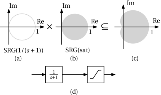
Figure 1: Bounding SRG for the composition of a first order lag and saturation.

3 Incremental robustness and sensitivity

3.1 Stability and incremental gain

Given the negative feedback interconnection of Figure 2, incremental stability is guaranteed by the separation of the SRGs of $P^{-1}$ and $-C$, and the distance between them is an incremental robustness margin, the reciprocal of which bounds the incremental gain of the feedback system. This is formalized in (Chaffey et al., 2021, Thm. 2); we recall the result here.

Figure 2: Negative feedback control structure.

Let $\mathcal{H}$ be a class of operators. By $\bar{\mathcal{H}}$, we will denote a class of operators such that $\mathcal{H}\subseteq\bar{\mathcal{H}}$ and $\operatorname{SRG}_{\,}({\bar{\mathcal{H}}})$ satisfies the chord property: if $z_{1},z_{2}\in\operatorname{SRG}_{\,}({\bar{\mathcal{H}}})$, then $\vartheta z_{1}+(1-\vartheta)z_{2}\in\operatorname{SRG}_{\,}({\bar{\mathcal{H}}})$ for all $\vartheta\in[0,1]$.

Theorem 3

Consider the feedback interconnection shown in Figure 2 between any pair of operators $C\in\mathcal{C}$ and $P\in\mathcal{P}$, where $\mathcal{C}$ and $\mathcal{P}$ are classes of operators on $L_{2}$ with finite incremental gain. If, for all $\tau\in(0,1]$, rCl $\operatorname{$}{SRG}_{\,}({\mathcal{C}})^{-1}\cap-\tau\operatorname{SRG}_{\,}({\bar{\mathcal{P}}})=\varnothing,thentheincremental$L_2$gainfrom$r$to$u$isboundedby$1/r_m$,where$r_m$istheshortestdistancebetween$$\operatorname{$}{SRG}_{\,}({\mathcal{C}^{-1}})$ and $-\operatorname{SRG}_{\,}({\bar{\mathcal{P}}})$.

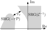
Figure 3: Illustration of Theorem 3.

3.2 The sensitivity SRG

The operator $(I+PC)^{-1}$ maps $r$ to $e$ in the feedback system of Figure 2, and the operator $(I-PC(-I))^{-1}$ maps $n$ to $y$. These two operators have the same SRG, which we denote by $\mathcal{S}$ – the sensitivity SRG.

Definition 4

The peak incremental sensitivity is the maximum incremental gain of the operator $(I+PC)^{-1}$.

The peak incremental sensitivity is equal to the maximum modulus of $\mathcal{S}$. The following theorem gives the peak incremental sensitivity an interpretation as a robustness margin.

Theorem 5

Let $s_{m}$ be the shortest distance between
$\operatorname{SRG}_{\,}({PC})$ and the point $-1$. Then the peak incremental sensitivity is equal to $1/s_{m}$.

4 Loop shaping

We demonstrate SRG loop shaping with two simple design examples for the control structure shown in Figure 2.

4.1 Shaping for stability and robustness

As first design example, we show how to use SRGs to ensure incremental stability of a closed loop system. Unlike traditional loop shaping, where the return ratio $L=PC$ is modified, we graphically shape the inverse of the feedback system, $(P+C^{-1})$, to improve the robustness of the closed loop. The use of SRGs makes the design close to classical Nyquist analysis, despite the nonlinearity of $P$.

Figure 4: Example control system. $\bar{P}=1/(s(s+1))$, $N$ is a nonlinear operator and $C$ is the controller, to be designed. $r$ is the reference input, $n$ represents sensor noise.

Consider the system in Figure 4. $C$ represents the controller, to be designed. Suppose that the process consists of $\bar{P}$ with LTI dynamics $1/(s(s+1))$, and a nonlinear operator $N$, whose SRG is known to be bounded in the region illustrated in Figure 1 (c). We denote $C\bar{P}$ by $L$. The controller $C$ is to be designed to stabilize the system and decrease the incremental gain.

To ensure stability, we require the SRGs of $L^{-1}=(C\bar{P})^{-1}$ and $-N$ to be separated, for all scalings of $N$ between $0$ and $1$ (following Theorem 3). With $C_{0}=1$, the closed loop is unstable, as shown in Figure 5 (a). Shifting $L^{-1}$ to the left, by designing $C$ to give $L^{-1}=s(s+1)+1$, gives a stabilizing control. The controller reads $C_{1}=s(s+1)/(1+s(s+1))$.

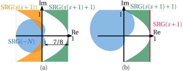
Figure 5: (a) SRGs of $-N$, $\bar{P}^{-1}$ and $(\bar{P}C_{1})^{-1}$. (b) SRGs of $(\bar{P}C_{1})^{-1}$, $(\bar{P}C_{2})^{-1}$ and a scaled and rotated nonlinearity, showing the improved robustness with $C_{2}$.

To improve robustness and reduce the incremental gain of the system, the separation of $\operatorname{SRG}_{\,}({L^{-1}})$ and $\operatorname{SRG}_{\,}({-N})$ must be increased (again, following Theorem 3). For example, setting $L^{-1}=s+1$ ($C_{2}=s$) gives good separation, and an incremental gain bound from $r$ to $u$ of $8/7\approx 1.14$. As the incremental gain of $N$ is bounded by $1$ (the maximum modulus of its SRG), this value also bounds the incremental gain from $r$ to $y$. The increased separation of the SRGs makes the system robust to uncertainties in the nonlinearity $N$, as illustrated in Figure 5 (b).

4.2 Shaping for performance

We now focus on graphical methods for improving performance, and explore how the sensitivity SRG can be shaped over particular sets of signals. We consider a new system, again of the form of Figure 2, with $C=1/(ks+1)$, where $k$ is a scalar to be designed, and $P$ is a unit saturation. The SRGs of $C$ and $P$ are shown in Figure 1 (a) and (b).

Tracking performance and noise rejection are both characterized by the sensitivity SRG. Suppose that we would like this SRG to have a low modulus (corresponding to incremental gain) for signals with a bandwidth of $\omega_{0}=10$ rad$/$s and a maximum amplitude of $2$. The aim is to limit the maximum amplification of $(I+PC)^{-1}$ over this range of signals.

A heuristic method is to maximize the distance between $\operatorname{SRG}_{\,}({PC})$ and $-1$ over the frequency range $[-\omega_{0},\omega_{0}]$ and amplitude range $[-2,2]$, following Theorem 5. This corresponds to maximizing the minimum incremental gain of the inverse of the sensitivity operator over this range of signals.

$\operatorname{SRG}_{\,}({PC})$ is bounded by the Minkowski product of $\operatorname{SRG}_{\,}({P})$ and $\operatorname{SRG}_{\,}({C})$. Plotting the SRG of the saturation $P$ over the amplitude range $[-2,2]$ gives the half-disc shown in Figure 6 (b). The SRG of $C$ over $[-\omega_{0},\omega_{0}]$ is described by rCl ( 11 + k2ω2, j -kω1 + k2ω2) for $\omega\in[-\omega_{0},\omega_{0}]$. As a first design, we can set $k$ so that the bandlimited SRG of $C$ is half the circle (Figure 6 (a)) – this is achieved by setting $k=0.01$. This gives the bound on $\operatorname{SRG}_{\,}({PC})$ shown in Figure 6 (c). The minimum distance to the point $-1$ is $s_{m}=\sqrt{3}$.

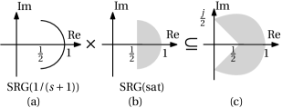
Figure 6: Left: SRG of $1/(ks+1)$ over signals with bandwidth $[-1/k,1/k]$. Right: SRG of saturation over signals with maximum amplitude $2$.

This method is, however, only a heuristic. The saturation introduces higher harmonics, so the assumption that signals have a bounded spectrum is invalidated when the loop is closed. However, given the lowpass properties of the system, the approximation is reasonable. The higher order harmonics of the output of the saturation have low magnitude, and the unit lag has a lowpass behavior. The stability of the closed loop guarantees that these high frequencies are indeed attenuated by the feedback system. This assumption is similar to the lowpass assumption of describing function analysis Slotine and Li (1991). The method here differs from describing function analysis, however, in that arbitrary differences of bandlimited inputs are considered, not just pure sinusoids.

5 Other types of systems

A significant advantage of the SRG is being able to place disparate system types on an equal footing. Like continuous time LTI systems, finite dimensional linear operators described by matrices lend themselves well to shaping. Pates (2021) has shown that the SRG of a matrix is equal to the numerical range of a closely related, transformed matrix. In the case of normal matrices, the SRG is the h-convex hull of the spectrum (Huang et al., 2020). These results pave the way for shaping a matrix’s SRG by matrix multiplication and addition.

In cases where the analytic SRG is not available, the SRG can be sampled over the signals of interest, and loop shaping methods can then be applied using the sampled SRG. For example, Figure 7 shows a sampled SRG of the potassium conductance of the Hodgkin-Huxley model of a neuron (Hodgkin and Huxley, 1952).

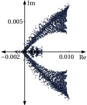
Figure 7: Sampling of the SRG of a potassium conductance.

References

- Bode (1960) Bode, H.W. (1960). Feedback – the history of an idea. In Proceedings of the Symposium on Active Networks and Feedback Systems, Microwave Research Institute Symposia Series. Polytechnic Press, Brooklyn.
- Chaffey (2022) Chaffey, T. (2022). A rolled-off passivity theorem. Systems & Control Letters, 162.
- Chaffey et al. (2021) Chaffey, T., Forni, F., and Sepulchre, R. (2021). Graphical nonlinear system analysis. arXiv:2107.11272 [cs, eess, math].
- Clegg (1958) Clegg, J.C. (1958). A nonlinear integrator for servomechanisms. Transactions of the American Institute of Electrical Engineers, Part II: Applications and Industry, 77(1), 41–42. 10.1109/TAI.1958.6367399.
- Hodgkin and Huxley (1952) Hodgkin, A.L. and Huxley, A.F. (1952). A quantitative description of membrane current and its application to conduction and excitation in nerve. The Journal of Physiology, 117(4), 500–544. 10.1113/jphysiol.1952.sp004764.
- Huang et al. (2020) Huang, X., Ryu, E.K., and Yin, W. (2020). Scaled relative graph of normal matrices. arXiv:2001.02061 [cs, math].
- McFarlane and Glover (1992) McFarlane, D. and Glover, K. (1992). A loop-shaping design procedure using H/sub infinity / synthesis. IEEE Transactions on Automatic Control, 37(6), 759–769. 10.1109/9.256330.
- Pates (2021) Pates, R. (2021). The scaled relative graph of a linear operator. arXiv:2106.05650 [math].
- Ryu et al. (2021) Ryu, E.K., Hannah, R., and Yin, W. (2021). Scaled relative graphs: Nonexpansive operators via 2D Euclidean geometry. Mathematical Programming. 10.1007/s10107-021-01639-w.
- Slotine and Li (1991) Slotine, J.J.E. and Li, W. (1991). Applied Nonlinear Control. Prentice Hall, Englewood Cliffs, N.J.
- Vinnicombe (2000) Vinnicombe, G. (2000). Uncertainty and Feedback: Loop-Shaping and the -Gap Metric. Imperial College Press.
- Zames (1981) Zames, G. (1981). Feedback and optimal sensitivity: Model reference transformations, multiplicative seminorms, and approximate inverses. IEEE Transactions on Automatic Control, 26(2), 301–320. 10.1109/TAC.1981.1102603.