Measurement of the $K_{S}\to\pi e\nu$ branching fraction with the KLOE experiment ^∗

Abstract

The ratio $\mathcal{R}=\Gamma(K_{S}\to\pi e\nu)/\Gamma(K_{S}\to\pi^{+}\pi^{-})$ has been measured with a sample of 300 million $K_{S}$ mesons produced in $\phi\to K_{L}K_{S}$ decays recorded by the KLOE experiment at the DA$\Phi$NE $e^{+}e^{-}$ collider. $K_{S}\to\pi e\nu$ events are selected by a boosted decision tree built with kinematic variables and time-of-flight measurements. Data control samples of $K_{L}\to\pi e\nu$ decays are used to evaluate signal selection efficiencies. With 49647$\pm$316 signal events we measure $\mathcal{R}=(1.0421\pm 0.0066_{\rm stat}\pm 0.0075_{\rm syst})\times 10^{-3}$. The combination with our previous measurement gives $\mathcal{R}=(1.0338\pm 0.0054_{\rm stat}\pm 0.0064_{\rm syst})\times 10^{-3}$. From this value we derive the branching fraction $\mathcal{B}(K_{S}\to\pi e\nu)=(7.153\pm 0.037_{\rm stat}\pm 0.044_{\rm syst})\times 10^{-4}$ and $f_{+}(0)|V_{us}|=0.2170\pm 0.009$.

1 Introduction

The branching fraction for semileptonic decays of charged and neutral kaons together with the lifetime measurements are used to determine the $|V_{us}|$ element of the Cabibbo–Kobayashi–Maskawa quark mixing matrix. The relation among the matrix elements of the first row, $|V_{ud}|^{2}+|V_{us}|^{2}+|V_{ub}|^{2}=1$, provides the most stringent test of the unitarity of the quark mixing matrix. At present, the sum $\sum_{i}|V_{ui}|^{2}$ differs from one by about $3\sigma$, an intriguing question under careful scrutiny, the so-called Cabibbo angle anomaly Grossman2020 .

Different factors contribute to the uncertainty in determining $|V_{us}|$ from kaon decays, discussed in Refs. ref:Antonelli2010 ; ref:Passemar2018 ; ref:PDGVus ; ref:VusUpdate , and among the six semileptonic decays the contribution of the lifetime uncertainty is smallest for the $K_{S}$ meson. Nevertheless, given the lack of pure high-intensity $K_{S}$ meson beams compared with $K^{\pm}$ and $K_{L}$ mesons, the measurements of $K_{S}$ semileptonic decays provide the least precise determination of $|V_{us}|$. Beside early measurements of $\mathcal{B}(K_{S}\to\pi e\nu)$ based on $\phi\to K_{L}K_{S}$ decays ref:CMD2 ; ref:KLOE2002 and the recent measurement of $\mathcal{B}(K_{S}\to\pi\mu\nu)$ ref:KStopimunu , the most precise measurements of the $K_{S}$ semileptonic branching fraction are from NA48: $\mathcal{B}(K_{S}\to\pi e\nu)=(7.05\pm 0.18_{\rm stat}\pm 0.16_{\rm syst})\times 10^{-4}$ ref:Na48 , and KLOE: $\mathcal{B}(K_{S}\to\pi e\nu)=(7.046\pm 0.091)\times 10^{-4}$ ref:KStopienu .

We present a new measurement of the ratio $\mathcal{R}=\frac{\Gamma(K_{S}\to\pi e\nu)}{\Gamma(K_{S}\to\pi^{+}\pi^{-})}$ performed by the KLOE experiment at the DA$\Phi$NE $\phi$–factory of the Frascati National Laboratory based on data collected in 2004–05 corresponding to an integrated luminosity of 1.63 fb^-1. DA$\Phi$NE ref:DAFNE is an electron–positron collider running at the centre-of-mass energy of $\sim$1.02 GeV colliding $e^{+}$ and $e^{-}$ beams at an angle of $\pi$$-$0.025 rad and with a bunch-crossing period of 2.715 ns. The $\phi$ mesons are produced with a small transverse momentum $p_{\phi}$ of $\sim$13 MeV and $K_{L}$–$K_{S}$ pairs are produced almost back-to-back with an effective cross section of $\sim$1 mb. The beam energy, the energy spread, the $\phi$ transverse momentum and the position of the interaction point are measured with high accuracy using Bhabha scattering events ref:Luminosity .

The $K_{S}$ ($K_{L}$) mesons are identified (tagged) with high efficiency and purity by the observation of a $K_{L}$ ($K_{S}$) in the opposite hemisphere. This tagging procedure allows the selection efficiency for $K_{S}\to\pi e\nu$ to be evaluated with good accuracy using a sample of the abundant decay $K_{L}\to\pi e\nu$ tagged by the detection of $K_{S}\to\pi^{+}\pi^{-}$ decays. The branching fraction $\mathcal{B}(K_{S}\to\pi e\nu)$ is obtained from the ratio $\mathcal{R}$ and the value of $\mathcal{B}(K_{S}\to\pi^{+}\pi^{-})$ measured by KLOE ref:KStopipi .

2 The KLOE detector

The detector consists of a large-volume cylindrical drift chamber, surrounded by a lead-scintillating fibers finely-segmented calorimeter. A superconducting coil around the calorimeter provides a 0.52 T axial magnetic field. The beam pipe at the interaction region is spherical in shape with 10 cm radius, made of a 0.5 mm thick beryllium–aluminium alloy. Low-beta quadrupoles are located at $\pm$50 cm from the interaction region. Two small lead-scintillating-tile calorimeters ref:QCAL are wrapped around the quadrupoles.

The drift chamber (DC) ref:DC , 4 m in diameter and 3.3 m long, has 12582 drift cells arranged in 58 concentric rings with alternated stereo angles and is filled with a low-density gas mixture of 90% helium–10% isobutane. The chamber shell is made of carbon fiber-epoxy composite with an internal wall of 1.1 mm thickness at 25 cm radius. The spatial resolution is $\sigma_{xy}=$ 0.15 mm and $\sigma_{z}=$ 2 mm in the transverse and longitudinal projection, respectively. The momentum resolution for tracks with polar angle $45^{\circ}<\theta<135^{\circ}$ is $\sigma_{p_{\rm T}}/p_{\rm T}=0.4\%$. Vertices formed by two tracks are reconstructed with a spatial resolution of about 3 mm.

The calorimeter (EMC) ref:EMC is divided into a barrel and two endcaps and covers 98% of the solid angle. The readout granularity is 4.4$\times$4.4 cm², for a total of 2440 cells arranged in five layers. Each cell is read out at both ends by photomultipliers. The energy deposits are obtained from signal amplitudes, the arrival times of particles and their position along the fibres are determined from the signals at the two ends. Cells close in space and time are grouped into energy clusters. The cluster energy $E$ is the sum of the cell energies, the cluster time and position are energy-weighted averages. Energy and time resolutions are $\sigma_{E}/E=0.057/\sqrt{E\ {\rm(GeV)}}$ and $\sigma_{t}=54\ {\rm ps}/\sqrt{E\ {\rm(GeV)}}\oplus 100$ ps, respectively. The cluster spatial resolution is $\sigma_{\parallel}=1.4\ {\rm cm}/\sqrt{E\ {\rm(GeV)}}$ along the fibres and $\sigma_{\perp}=1.3$ cm in the orthogonal direction.

The level-1 trigger ref:Trigger uses both the calorimeter and the drift chamber information; the calorimeter trigger requires two energy deposits with $E>50$ MeV in the barrel and $E>150$ MeV in the endcaps; the drift chamber trigger is based on the number and topology of hit drift cells. A higher-level cosmic-ray veto rejects events with at least two energy deposits above 30 MeV in the outermost calorimeter layer. The trigger time is determined by the first particle reaching the calorimeter and is synchronised with the DA$\Phi$NE r.f. signal. The time interval between bunch crossings is smaller than the time spread of the signals produced by the particles, thus the event T₀ related to the bunch crossing originating the event is determined after event reconstruction and all the times related to that event are shifted accordingly. Data for reconstruction are selected by an on-line filter ref:Datarec to reject beam backgrounds. The filter also streams the events into different output files for analysis according to their properties and topology. A fraction of 5% of the events are recorded without applying the filter to control inefficiencies in the event streaming.

The KLOE Monte Carlo (MC) simulation package, GEANFI ref:Datarec , has been used to produce an event sample equivalent to the data. Energy deposits in EMC and DC hits from beam background events triggered at random are overlaid onto the simulated events which are then processed with the same reconstruction algorithms as the data.

3 The measurement of $\Gamma(K_{S}\to\pi e\nu)/\Gamma(K_{S}\to\pi^{+}\pi^{-})$

The ratio of $\Gamma(K_{S}\to\pi e\nu)$ to $\Gamma(K_{S}\to\pi^{+}\pi^{-})$ is evaluated as

$$\mathcal{R}=\frac{\Gamma(K_{S}\to\pi e\nu)}{\Gamma(K_{S}\to\pi^{+}\pi^{-})}=\frac{N_{\pi e\nu}}{\epsilon_{\pi e\nu}}\times\frac{\epsilon_{\pi\pi}}{N_{\pi\pi}}\times R_{\epsilon},$$ (1)

where $N_{\pi e\nu}$ and $N_{\pi\pi}$ are the numbers of selected $K_{S}\to\pi e\nu$ and $K_{S}\to\pi^{+}\pi^{-}$ events, $\epsilon_{\pi e\nu}$ and $\epsilon_{\pi\pi}$ are the respective selection efficiencies, and $R_{\epsilon}=(\epsilon_{\pi\pi}/\epsilon_{\pi e\nu})_{\rm com}$ is the ratio of common efficiencies for the trigger, on-line filter, event classification and preselection that can be different for the two decays.

The number of signal events, $N_{\pi e\nu}$ in Eq. (1), is the sum of the two charge-conjugated decays to $\pi^{-}e^{+}\nu$ and $\pi^{+}e^{-}\bar{\nu}$. These are separated in a parallel analysis of the same dataset based on the same selection criteria presented in this section, optimised for measuring the charge asymmetry $\frac{\Gamma(\pi^{-}e^{+}\nu)-\Gamma(\pi^{+}e^{-}\bar{\nu})}{\Gamma(\pi^{-}e^{+}\nu)+\Gamma(\pi^{+}e^{-}\bar{\nu})}$ ref:KStopienuAsimmetry .

3.1 Data sample and event preselection

Neutral kaons from $\phi$-meson decays are emitted in two opposite hemispheres with $\lambda_{S}=5.9$ mm and $\lambda_{L}=3.4$ m mean decay path for $K_{S}$ and $K_{L}$ respectively. About 50% of $K_{L}$ mesons reach the calorimeter before decaying and the $K_{L}$ velocity in the $\phi$-meson reference system is $\beta^{*}=0.22$. $K_{S}$ mesons are tagged by $K_{L}$ interactions in the calorimeter, $K_{L}$–crash in the following, with a clear signature of a delayed cluster not associated to tracks. To select $K_{L}$–crash and then tag $K_{S}$ mesons, the requirements are:

• one cluster not associated to tracks (neutral cluster) and with energy $E_{\rm clu}>100$ MeV, the centroid of the neutral cluster defining the $K_{L}$ direction with an angular resolution of $\sim$1^∘;

• $15^{\circ}<\theta_{\rm clu}<165^{\circ}$ for the polar angle of the neutral cluster, to suppress small-angle beam backgrounds;

• $0.17<\beta^{*}<0.28$ for the velocity in the $\phi$ reference system of the $K_{L}$ candidate; $\beta^{*}$ is obtained from the velocity in the laboratory system, $\beta=r_{\rm clu}/ct_{\rm clu}$, with $t_{\rm clu}$ being the cluster time and $r_{\rm clu}$ the distance from the nominal interaction point, the $\phi$-meson momentum and the angle between the $\phi$-meson momentum and the $K_{L}$–crash direction.

The $K_{S}$ momentum $\vec{p}_{K_{S}}=\vec{p}_{\phi}-\vec{p}_{K_{L}}$ is determined with an accuracy of 2 MeV, assigning the neutral kaon mass.

$K_{S}\to\pi e\nu$ and $K_{S}\to\pi^{+}\pi^{-}$ candidates are preselected requiring two tracks of opposite curvature forming a vertex inside the cylinder defined by

$$\rho_{\rm vtx}=\sqrt{x^{2}_{\rm vtx}+y^{2}_{\rm vtx}}<5\ {\rm cm}\qquad|z_{\rm vtx}|<10\ {\rm cm}.$$ (2)

After preselection, the data sample contains about 300 million events and its composition evaluated by simulation is shown in Table 1. The large majority of events are $K_{S}\to\pi^{+}\pi^{-}$ decays, together with a large contribution from $\phi\to K^{+}K^{-}$ events where one kaon produces a track and the kaon itself or its decay products generate a fake $K_{L}$–crash while the other kaon decays early into $\pi^{\pm}\pi^{0}$.

Table 1: Number of events for data and simulation after $K_{L}$–crash and $K_{S}$ preselection.

	Events	Fraction [%]
Data	301 645 500
MC	312 018 500
$\phi\to K_{L}K_{S},K_{S}\to\pi e\nu$	259 264	0.08
$\phi\to K_{L}K_{S},K_{S}\to\pi^{+}\pi^{-}$	301 976 400	96.78
$\phi\to K^{+}K^{-}$	9 565 465	3.07
$\phi\to K_{L}K_{S},K_{S}\to\pi\mu\nu$	139 585	0.04
$\phi\to K_{L}K_{S},K_{S}\to\pi^{0}\pi^{0}$	30 353	0.01
$\phi\to K_{L}K_{S},K_{S}\to\pi^{+}\pi^{-}e^{+}e^{-}$	18 397	0.006
$\phi\to\pi^{+}\pi^{-}\pi^{0}$	24 153	0.008
others	4 852	0.002

The $\beta^{*}$ distribution is shown in Figure 1, for data and simulated events. Two peaks are visible, the first is associated to events triggered by photons or electrons, and the second to events triggered by charged pions. The trigger is synchronised with the bunch crossing and the time difference between an electron (or photon) and a pion (or muon) arriving at the calorimeter corresponds to about one bunch-crossing shift.

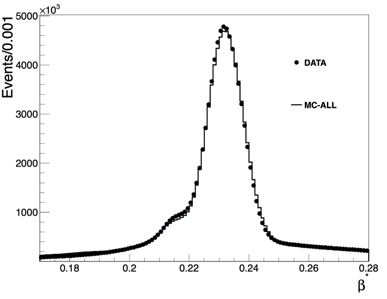
Figure 1: Distribution of $\beta^{*}$ after preselection for data and simulated events.

3.2 Signal selection and normalisation sample

Signal selection is performed in two steps based on uncorrelated information: 1) the event kinematics using only DC tracking variables, and 2) the time-of-flight measured with the EMC.

Time assignment to tracks requires track-to-cluster association (TCA): for each track connected to the vertex a cluster with $E_{\rm clu}>20$ MeV and $15^{\circ}<\theta_{\rm clu}<165^{\circ}$ is required whose centroid is within 30 cm of the track extrapolation inside the calorimeter. Track-to-cluster association is required for both tracks in the event.

A multivariate analysis is performed with a boosted decision tree (BDT) classifier built with the following five variables with good discriminating power against background:

• : the tracks momenta;

• : the angle at the vertex between the two momenta in the $K_{S}$ reference system;

• : the angle between the momentum sum, $\vec{p}_{\rm sum}=\vec{p}_{1}+\vec{p}_{2}$, and the $K_{L}$–crash direction;

• : the difference between $|\vec{p}_{\rm sum}|$ and the absolute value $|\vec{p}_{K_{S}}|$ of the $K_{S}$ momentum;

• : the invariant mass reconstructed from $\vec{p}_{1}$ and $\vec{p}_{2}$, in the hypothesis of charged-pion mass.

Figure 2 shows the distributions of the variables for data and simulated signal and background events. Two selection cuts are applied to avoid regions far away from the signal where MC does not reproduce well the data:

$$p<320{\rm\ MeV\ for\ both\ tracks}\qquad{\rm and}\qquad\Delta p<190{\rm\ MeV.}$$ (3)

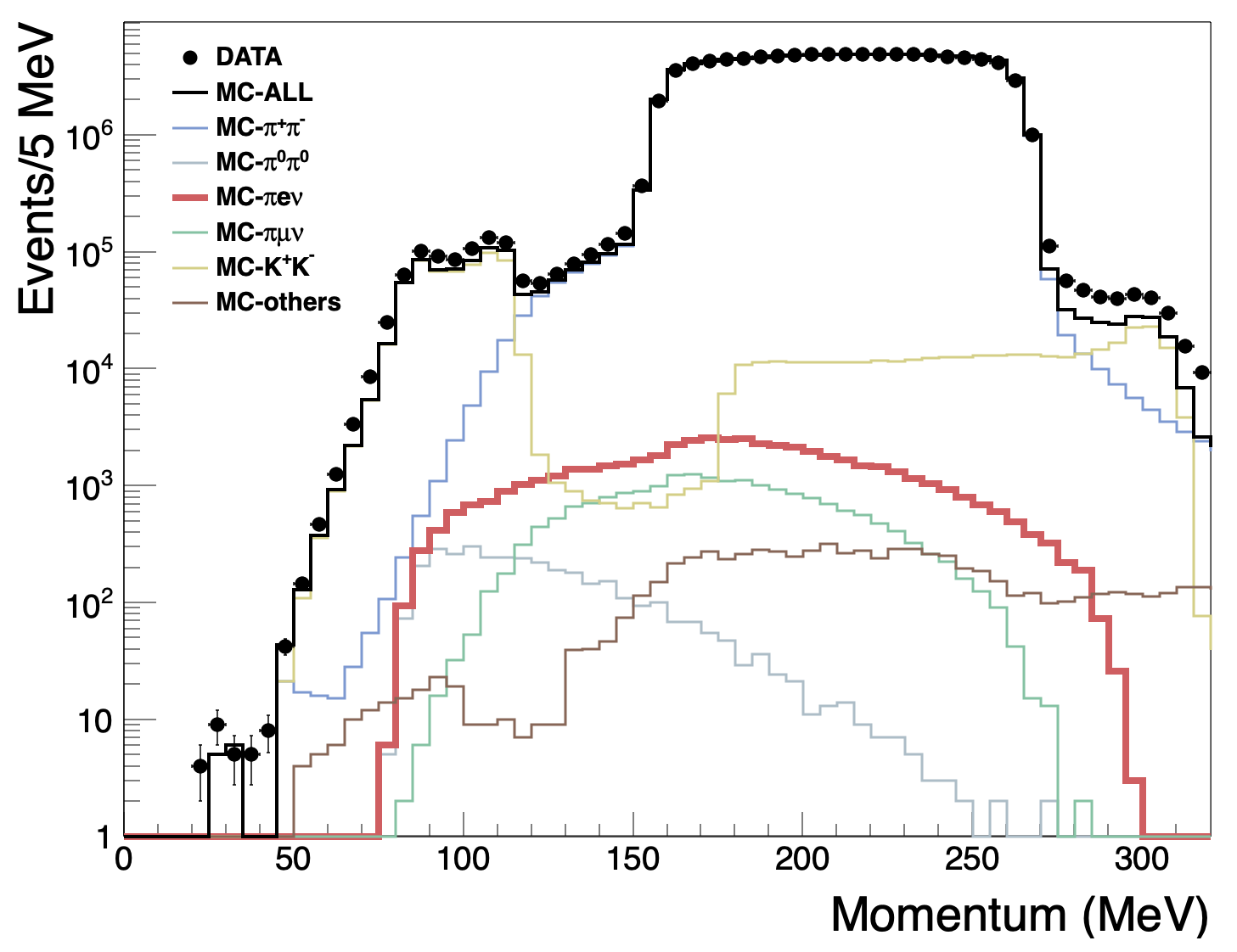
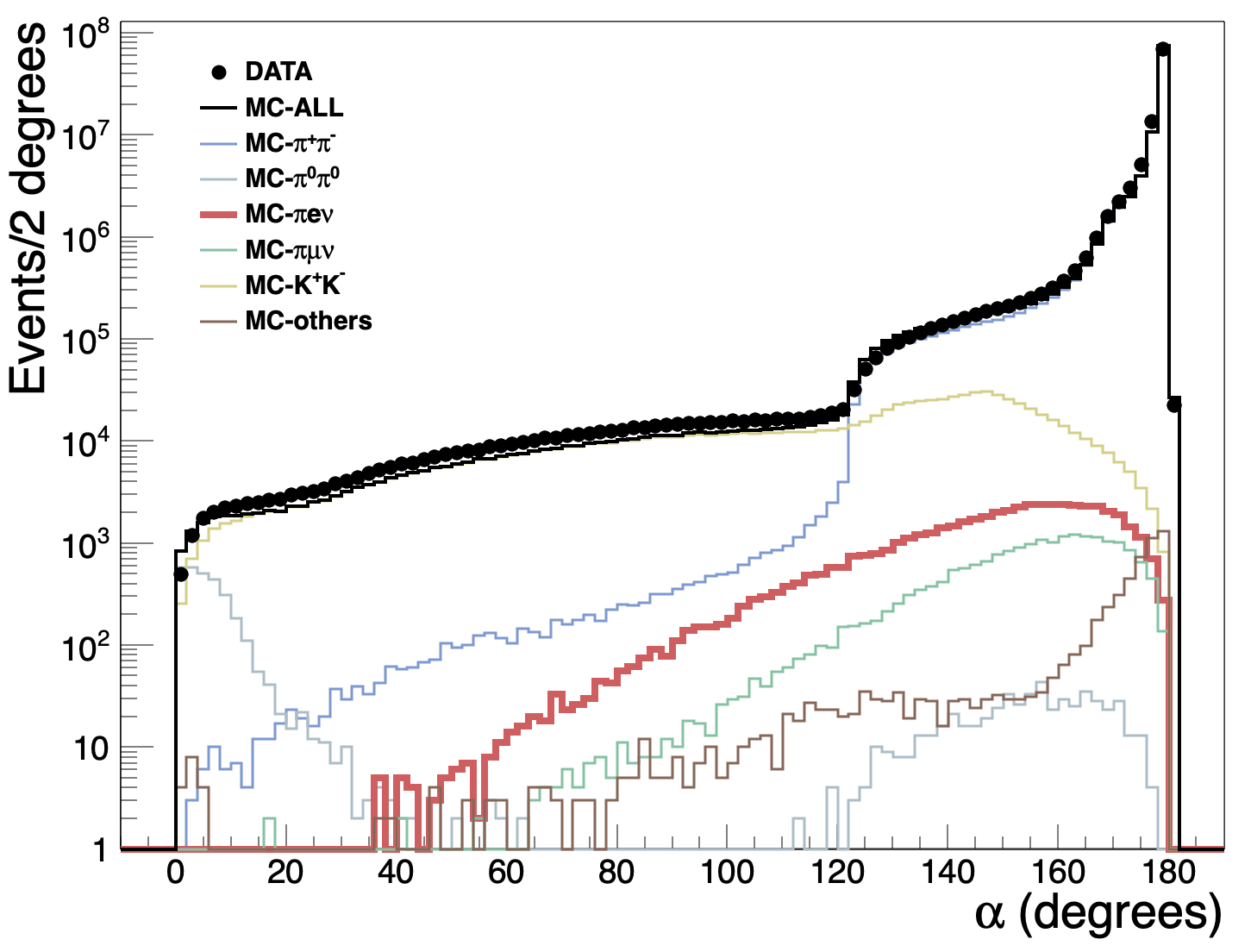
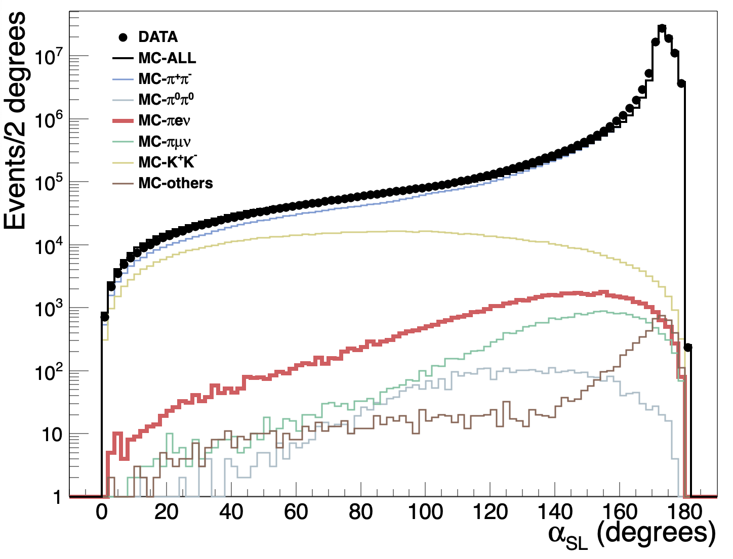
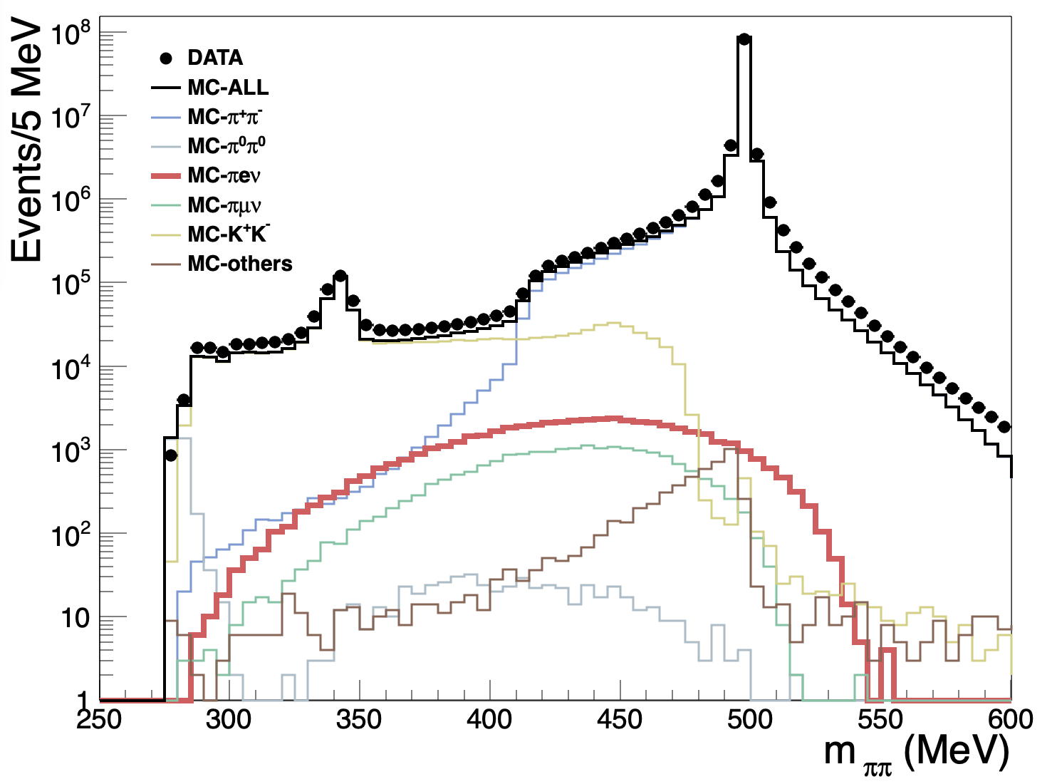
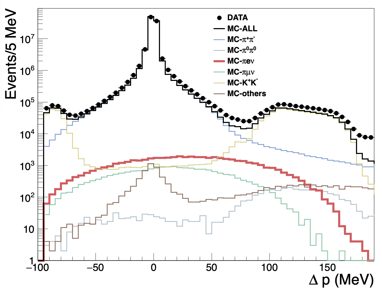
Figure 2: Distributions of the variables used in the multivariate analysis for data and simulated events after preselection. From top left: track momenta ($p_{1},p_{2}$), angle between the two tracks in the $K_{S}$ reference system ($\alpha_{1,2}$), angle beween $K_{L}$ and $K_{S}$ directions ($\alpha_{SL}$), two-track invariant mass in the hypothesis of charged pions ($m_{\pi\pi}$), $\Delta p=|\vec{p}_{\rm sum}|-|\vec{p}_{K_{S}}|$.

Training of BDT classifier is done with MC samples: 5,000 $K_{S}\to\pi e\nu$ events and 50,000 background events. Samples of the same size are used for the test. After training and test the classification is run on both MC and data samples. Figure 3 shows the BDT classifier output for data and simulated signal and background events. To suppress the large background contribution from $K_{S}\to\pi^{+}\pi^{-}$ and $\phi\to K^{+}K^{-}$ events, a cut is applied on the classifier output:

$$BDT>0.15.$$ (4)

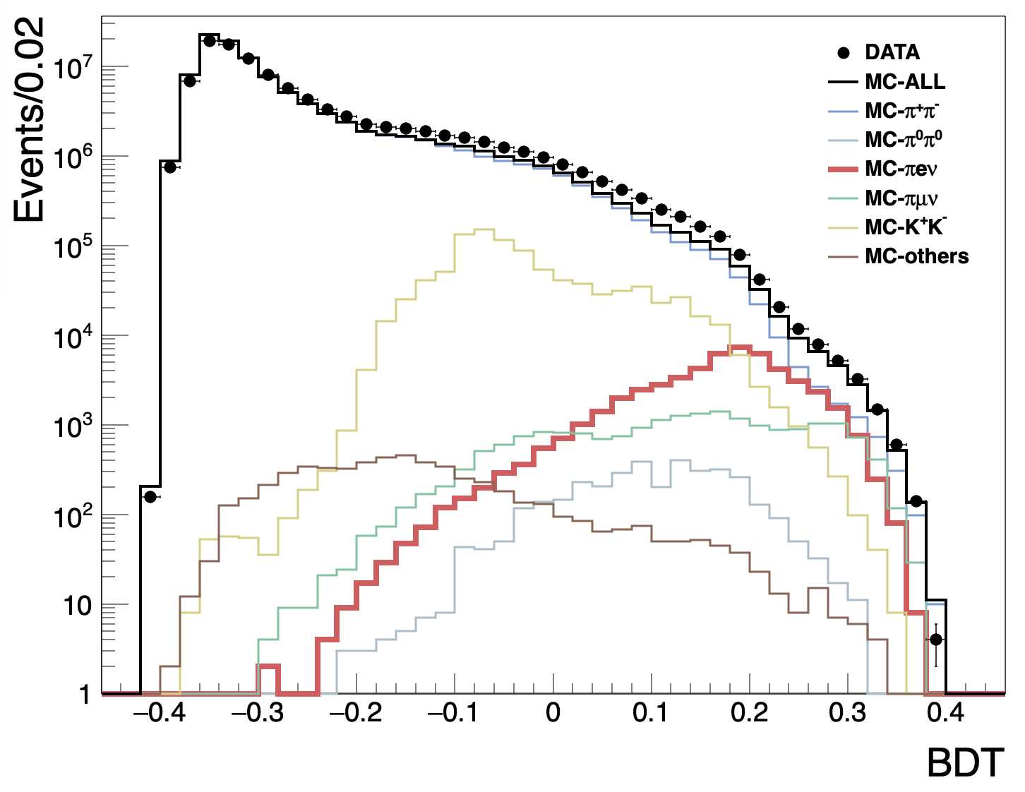
Figure 3: Distribution of the BDT classifier output for data and simulated signal and background events.

Track pairs in the selected events are $e\pi$ for the signal and are $K\pi$, $\pi\pi$, $\mu\pi$ for the main backgrounds. A selection based on time-of-flight measurements is performed to identify $e\pi$ pairs. For each track associated to a cluster, the difference between the time-of-flight measured by the calorimeter and the flight time measured along the particle trajectory

$$\delta t_{i}=t_{{\rm clu},i}-L_{i}/c\beta_{i}\qquad i=1,2$$ (5)

is computed, where $t_{{\rm clu},i}$ is the time associated to track $i$, $L_{i}$ is the length of the track, and the velocity $\beta_{i}=p_{i}/\sqrt{p_{i}^{2}+m_{i}^{2}}$ is function of the mass hypothesis for the particle with track $i$. The times $t_{{\rm clu},i}$ are referred to the trigger and the same T₀ value is assigned to both clusters. To reduce the uncertainty from the determination of T₀ the difference

$$\delta t_{1,2}=\delta t_{1}-\delta t_{2}$$

is used to determine the mass assignment. The $\pi\pi$ hypothesis is tested first. Figure 4 shows the $\delta t_{\pi\pi}=\delta t_{1,\pi}-\delta t_{2,\pi}$ distribution. A fair agreement is observed between data and simulation, with $K_{S}\to\pi e\nu$ and $K_{S}\to\pi\mu\nu$ distributions well separated and large part of the $K^{+}K^{-}$ background isolated in the tails of the distribution. However the signal is hidden under a large $K_{S}\to\pi^{+}\pi^{-}$ background, therefore a cut

$$2.5\ {\rm ns}<|\delta t_{\pi\pi}|<10\ {\rm ns}$$ (6)

is applied.

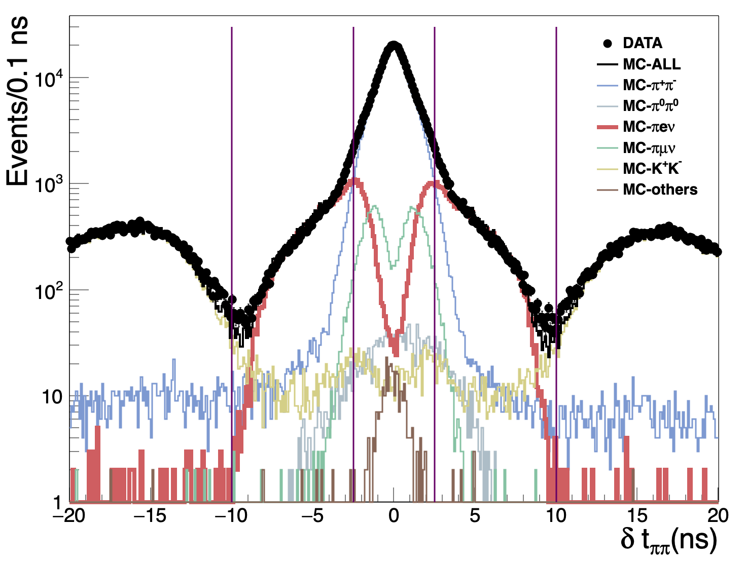
Figure 4: Distributions of $\delta t_{\pi\pi}$ for data and simulated signal and background events. The vertical lines indicate the selected range 2.5 ns $<|\delta t_{\pi\pi}|<$ 10 ns.

Then, the $\pi e$ hypothesis is tested by assigning the pion and electron mass to either track defining

$$\delta t_{\pi e}=\delta t_{1,\pi}-\delta t_{2,e}\qquad{\rm and}\qquad\delta t_{e\pi}=\delta t_{1,e}-\delta t_{2,\pi},$$

where the label as track-1 and track-2 is chosen at random. Figure 5 shows the two-dimensional $(\delta t_{\pi e},\delta t_{e\pi})$ distribution for data and MC where signal events populate either band around $\delta t=0$.

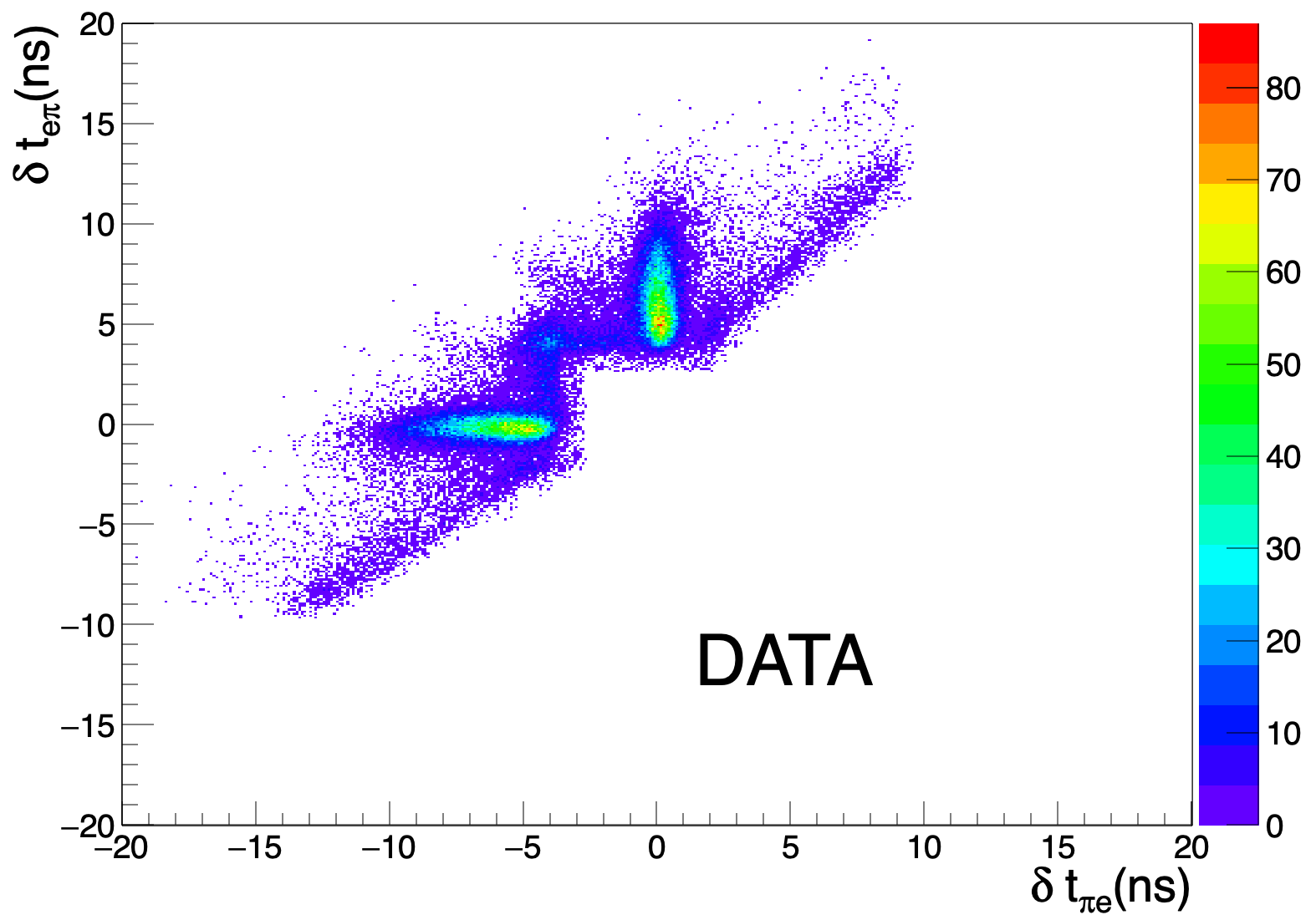
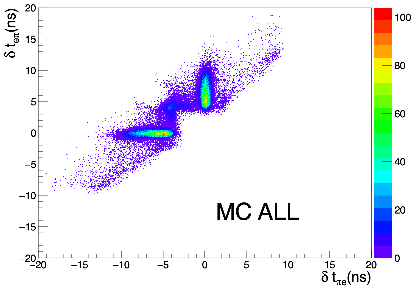
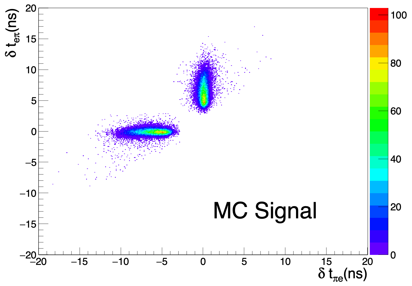
Figure 5: Two dimensional distribution $(\delta t_{\pi e},\delta t_{e\pi})$ for top: data and MC all, bottom: MC signal.

The mass assignment is based on the comparison of two hypotheses: if $|\delta t_{1,\pi}-\delta t_{2,e}|<|\delta t_{1,e}-\delta t_{2,\pi}|$ track-1 is assigned to the pion and track-2 to the electron, otherwise the other solution is taken; the corresponding time difference, $\delta t_{e}$, is the value defined by $\texttt{min}[|\delta t_{\pi e}|,|\delta t_{e\pi}|]$. A cut is applied on this variable

$$|\delta t_{e}|<1\ {\rm ns}.$$ (7)

The number of events selected by the time-of-flight requirements is 57577 and the composition as predicted by simulation is listed in Table 2. The background comprises $K_{S}\to\pi^{+}\pi^{-}$, $\phi\to K^{+}K^{-}$ and $K_{S}\to\pi\mu\nu$, the other contributions being small.

Table 2: Number of events after the BDT and TOF selections.

	Events	Fraction [%]
Data	57 577
MC	56 843
$\phi\to K_{L}K_{S},K_{S}\to\pi e\nu$	53 559	94.22
$\phi\to K_{L}K_{S},K_{S}\to\pi^{+}\pi^{-}$	2 175	3.83
$\phi\to K^{+}K^{-}$	903	1.59
$\phi\to K_{L}K_{S},K_{S}\to\pi\mu\nu$	136	0.24
others	70	0.12

The mass of the charged secondary identified as the electron is evaluated as

$$m_{e}^{2}=\left(E_{K_{S}}-E_{\pi}-p_{\rm miss}\right)^{2}-p^{2}_{e}$$

with $p_{\rm miss}^{2}=(\vec{p}_{K_{S}}-\vec{p}_{\pi}-\vec{p}_{e})^{2}$, $E_{K_{S}}$ and $\vec{p}_{K_{S}}$ being the energy and momentum reconstructed using the tagging $K_{L}$, and $\vec{p}_{\pi}$, $\vec{p}_{e}$, the momenta of the pion and electron tracks, respectively.

A fit to the $m_{e}^{2}$ distribution with the MC shapes of three components, $K_{S}\to\pi e\nu$, $K_{S}\to\pi^{+}\pi^{-}$ and the sum of all other backgrounds, allows the number of signal events to be extracted. The fit is performed in 100 bins in the range [-30000,+30000] MeV². Figure 6 shows the $m_{e}^{2}$ distribution for data and simulated events before the fit, and the comparison of the fit output with the data. The fit result is reported in Table 3. The number of signal events is

$$N_{\pi e\nu}=49647\pm 316\qquad{\rm with}\ \chi^{2}/{\rm ndf}=76/96.$$

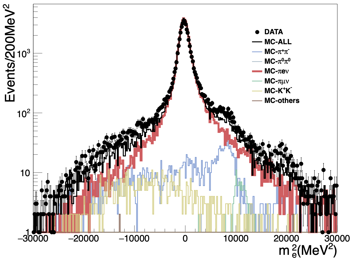
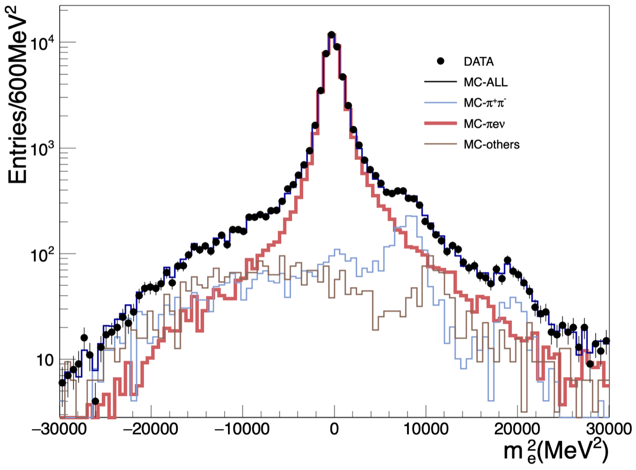
Figure 6: The $m_{e}^{2}$ distribution for data, MC signal and background before the fit (left) and comparison of data with the result of the fit (right).

Table 3: Result of the fit to the $m_{e}^{2}$ distribution.

	Fraction	Events
$\pi e\nu$	0.8651 $\pm$ 0.0055	49 647 $\pm$ 316
$\pi^{+}\pi^{-}$	0.0763 $\pm$ 0.0068	4 379 $\pm$ 390
all others	0.0586 $\pm$ 0.0067	3 363 $\pm$ 384
Total		57 389
$\chi^{2}$/ndf	76/96

The $K_{S}\to\pi^{+}\pi^{-}$ normalisation sample is selected requiring $K_{L}$–crash, two opposite curvature tracks, the vertex as in Eq. (2) and $140<p<280$ MeV for both tracks (Figure 2(a)). A total of $N_{\pi\pi}=(282.314\pm 0.017)\times 10^{6}$ events are selected with an efficiency of 97.4% and a purity of 99.9% as determined by simulation.

3.3 Determination of efficiencies

The signal efficiency for a given selection is determined with a $K_{L}\to\pi e\nu$ control sample (CS) and evaluated as

$$\epsilon_{\pi e\nu}=\epsilon_{\rm CS}\times\frac{\epsilon^{\rm MC}_{\pi e\nu}}{\epsilon^{\rm MC}_{\rm CS}},$$ (8)

where $\epsilon_{\rm CS}$ is the efficiency of the control sample, and $\epsilon^{\rm MC}_{\pi e\nu}$, $\epsilon^{\rm MC}_{\rm CS}$ are the efficiencies obtained from simulation for the signal and the control sample, respectively. Extensively studied with the KLOE detector ref:KLtoany , $K_{L}\to\pi e\nu$ decays are kinematically identical to the signal, the only difference being the much longer decay path. Tagging is done with $K_{S}\to\pi^{+}\pi^{-}$ decays selected requiring two opposite curvature tracks and the vertex defined in Eq. (2) with the additional requirement $|m_{\pi\pi}-m_{K^{0}}|<15$ MeV to increase the purity, ensuring the angular and momentum resolutions are similar to the $K_{L}$–crash tagging for the signal. The radial distance of the $K_{L}$ vertex is required to be smaller than 5 cm, to match the signal selection, but greater than 1 cm to minimise the ambiguity in identifying $K_{L}$ and $K_{S}$ vertices. Weighting the $K_{L}$ vertex position to emulate the $K_{S}$ vertex position has negligible effect on the result.

The control sample composition is $K_{L}\to\pi e\nu$ ($\mathcal{B}=0.405$), $K_{L}\to\pi\mu\nu$ ($\mathcal{B}=0.270$) and $K_{L}\to\pi^{+}\pi^{-}\pi^{0}$ ($\mathcal{B}=0.125$) decays, while most of $K_{L}\to\pi^{0}\pi^{0}\pi^{0}$ decays are rejected requiring two tracks and the vertex. The distribution of the $m^{2}_{\rm miss}$ missing mass, with respect to the two tracks connected to the $K_{L}$ vertex and in the charged-pion mass hypothesis, shows a narrow isolated peak at the $\pi^{0}$ mass. $K_{L}\to\pi^{+}\pi^{-}\pi^{0}$ decays are efficiently rejected with the $m^{2}_{\rm miss}<15000$ MeV² cut.

Two control samples are selected, based on the two-step analysis strategy using largely uncorrelated variables and presented in Section 3.2: the first CS_kinBDT applying a cut on the TOF variables to evaluate the efficiency of the selection based on the kinematic variables and the BDT classifier, the second CS_TCATOF applying a cut on kinematic variables to evaluate TCA and TOF selection efficiencies.

The CS_kinBDT control sample is selected applying a cut on the two-dimensional $(\delta t_{\pi e},\delta t_{e\pi})$ distribution, rejecting most of the $K_{L}\to\pi\mu\nu$ events. The sample contains $0.44\times 10^{6}$ events with a 97% purity as determined from simulation. The Monte Carlo BDT distributions for the signal and control sample are compared in Figure 7(left). Applying to the control sample the same selections as for the signal, Eqs. (3) and (4), the efficiencies evaluated with Eq. (8) are

$$\epsilon({\rm kin})=0.9720\pm 0.0007_{\rm stat}\qquad{\rm and}\qquad\epsilon({\rm BDT})=0.6534\pm 0.0013_{\rm stat}.$$

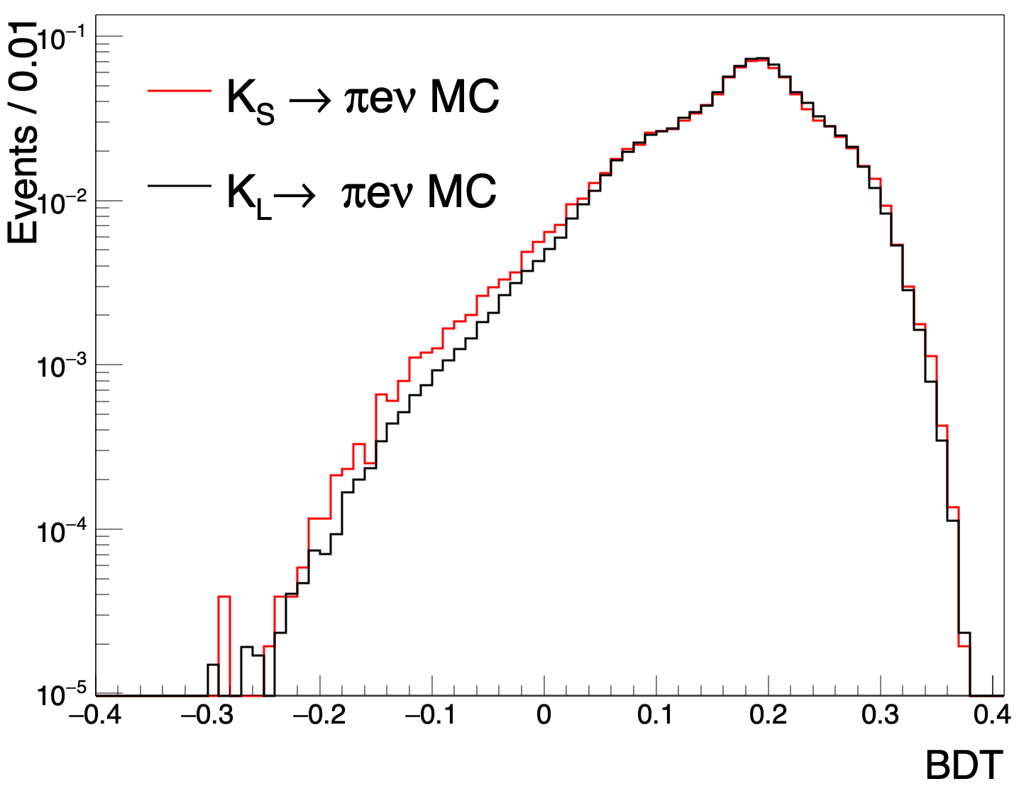
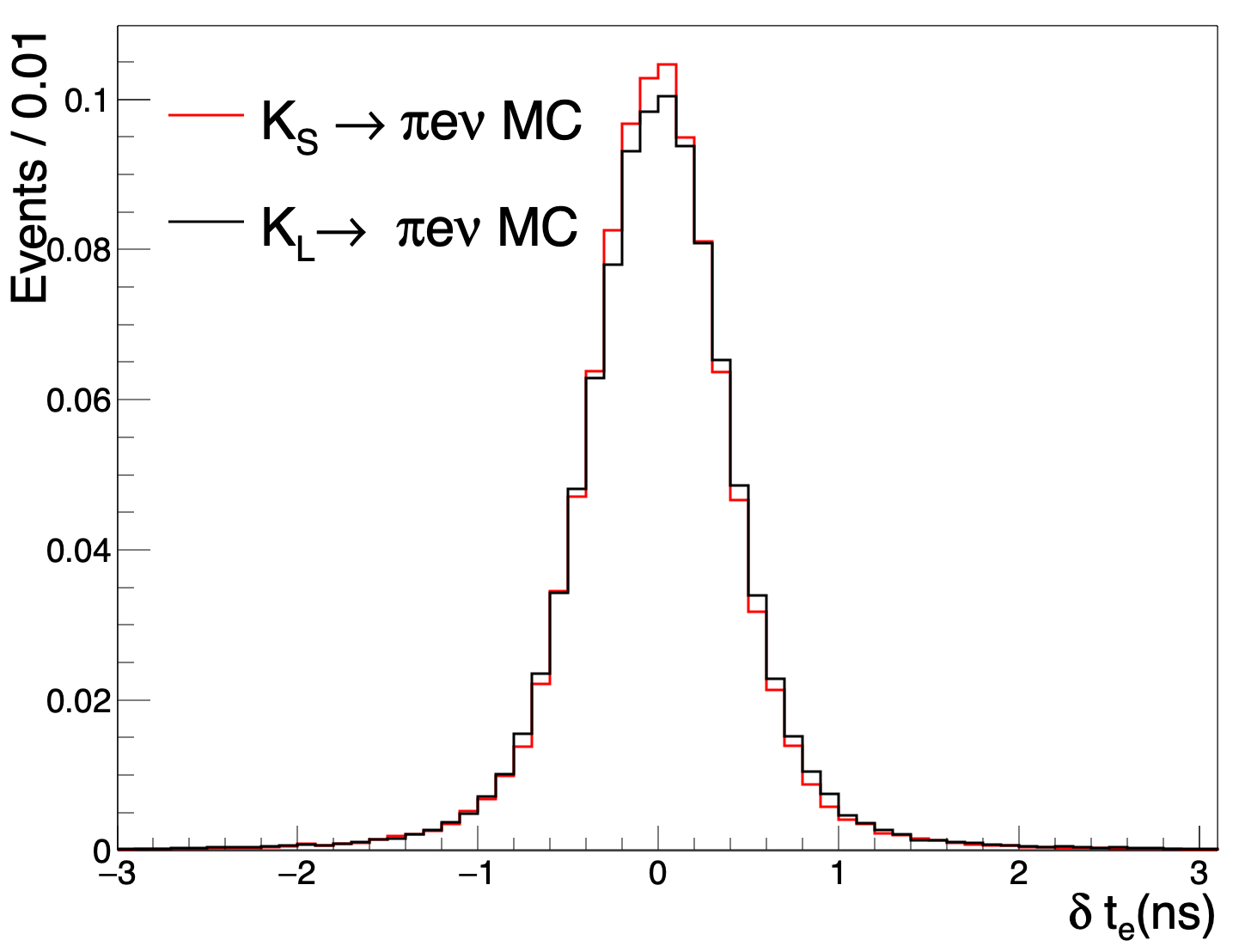
Figure 7: Monte Carlo distributions of the BDT classifier output (left) and $\delta t_{e}$ (right) for $K_{L}\to\pi e\nu$ (black) and $K_{S}\to\pi e\nu$ (red) events.

The CS_TCATOF control sample is selected applying a cut on the $(m_{\pi\pi},m^{2}_{\rm miss})$ distribution. The sample contains $1.3\times 10^{6}$ events with a 95% purity as determined from simulation. In the $K_{S}\to\pi e\nu$ analysis, the T₀ is determined by the first cluster in time, associated with one of the tracks of the $K_{S}$ decay. Then, for the control sample the first cluster in time is required to be associated with the $K_{L}$ decay, in order not to bias TOF variables. Figure 7(right) shows the comparison between the Monte Carlo distributions of $\delta t_{e}$ for signal and control sample. Applying to the control sample the same selections as for the signal, Eqs. (6) anf (7), the efficiencies evaluated with Eq. (8) are

$$\epsilon({\rm TCA})=0.4639\pm 0.0009_{\rm stat}\qquad{\rm and}\qquad\epsilon({\rm TOF})=0.6605\pm 0.0012_{\rm stat}.$$

Table 4 summarises the signal selection efficiencies.

Table 4: Signal selection efficiencies with statistical uncertainties. Correlations are accounted for in evaluating the total efficiency uncertainty.

Selection	Efficiency
Preselection (from MC)	0.9961 $\pm$ 0.0002
Kin. variables selection	0.9720 $\pm$ 0.0007
BDT selection	0.6534 $\pm$ 0.0013
TCA selection	0.4639 $\pm$ 0.0009
TOF selection	0.6605 $\pm$ 0.0012
Total	0.1938 $\pm$ 0.0006

For the $K_{S}\to\pi^{+}\pi^{-}$ normalisation sample, the efficiency of the momentum selection $140<p<280$ MeV is determined using preselected data. The cut on the vertex transverse position in Eq. (2) is varied in 1 cm steps from $\rho^{\rm max}_{\rm vtx}=1$ cm to $\rho^{\rm max}_{\rm vtx}=4$ cm, based on the observation that $\rho_{\rm vtx}$ and the tracks momenta are the least correlated variables, the correlation coefficient being 13%. Using Eq. (8) and extrapolating to $\rho^{\rm max}_{\rm vtx}=5$ cm, the efficiency is $\epsilon^{\rm data}_{\pi\pi}=(96.569\pm 0.004)\%$. Alternatively, the efficiency is evaluated using the $K_{S}\to\pi^{+}\pi^{-}$ data sample (with $\rho^{\rm max}_{\rm vtx}=5$ cm and $\epsilon^{\rm MC}_{\pi\pi}=\epsilon^{\rm MC}_{\rm pres}$), the efficiency is $\epsilon^{\rm data}_{\pi\pi}=(96.657\pm 0.002)\%$. The second value, free from bias of variables correlation, is used for the efficiency and the difference between the two values is taken as systematic uncertainty. The number of $K_{S}\to\pi^{+}\pi^{-}$ events corrected for the efficiency is $N_{\pi\pi}/\epsilon_{\pi\pi}=(292.08\pm 0.27)\times 10^{6}$.

The ratio $R_{\epsilon}$ in Eq. (1) includes several effects depending on the event global properties: trigger, on-line filter, event classification, T₀ determination, $K_{L}$–crash and $K_{S}$ identification. In Table 5 the various contributions to $R_{\epsilon}$ evaluated with simulation are listed with statistical uncertainties only, the resulting value is $R_{\epsilon}=1.1882\pm 0.0017$. Systematic uncertainties are detailed in Section 4.

Table 5: Ratios of MC efficiencies common to the $K_{S}\to\pi e\nu$ and $K_{S}\to\pi^{+}\pi^{-}$ selections with statistical uncertainties. The error on $R_{\epsilon}$ is calculated as the quadratic sum of the errors of the single ratios.

Selection	$R_{\epsilon}=(\epsilon_{\pi\pi}/\epsilon_{\pi e\nu})_{\rm com}$
Trigger	1.0297 $\pm$ 0.0003
On-line filter	1.0054 $\pm$ 0.0001
Event classification	1.0635 $\pm$ 0.0004
T0 time	1.0063 $\pm$ 0.0001
$K_{L}$–crash	1.0295 $\pm$ 0.0010
$K_{S}$ vertex reconstr.	1.0418 $\pm$ 0.0009
$R_{\epsilon}$	1.1882 $\pm$ 0.0017

4 Systematic uncertainties

The signal count is affected by three main systematic uncertainties: BDT selection, TOF selection, and the $m^{2}_{e}$ fit.

The distributions of the BDT classifier output for the data and simulated signal and control sample events are shown in Figures 3 and 7. The resolution of the BDT variable predicted by simulation comparing the reconstructed events with those at generation level is $\sigma_{\rm BDT}=0.005$. The analysis is repeated varying the BDT cut in the range 0.135–0.17. The ratio of the number of signal events determined with the $m_{e}^{2}$ fit and the efficiency evaluated with Eq. (8) is found to be stable and the half-width of the band defined by the maximum and minimum values, $\pm$0.27%, is taken as relative systematic uncertainty.

The number of reconstructed clusters can be different for the signal ($K_{L}$–crash,$\pi e\nu$) and control sample ($\pi\pi$,$\pi e\nu$), thus the TCA efficiency calculation is repeated by weighting the events of the control sample by the number of track-associated clusters. The difference, less than 0.1%, is taken as relative systematic uncertainty for the TCA efficiency.

The main source of uncertainty in the TOF selection is the lower cut on $|\delta t_{\pi\pi}|$ in Eq. (6) because the signal and background distributions in Figure 4 are steep and with opposite slopes. The resolution is the combination of the time resolution of the calorimeter, the tracking resolution of the drift chamber and the track-to-cluster association and is determined by the width of the $\delta t_{e}$ distribution.

The comparison of the $\delta t_{e}$ distributions for the signal and the $K_{L}\to\pi e\nu$ control sample is shown in Figure 8, they are fitted with a Gaussian and a $2^{nd}$ degree polynomial, obtaining $\sigma=0.44\pm 0.02$ ns in both cases. The analysis is repeated varying the $|\delta t_{\pi\pi}|$ lower cut in the range 2.0–3.0 ns, the half-width of the band gives a relative systematic uncertainty of $\pm$0.28%. With the same procedure the cut on $|\delta t_{e}|$ in Eq. (7) is varied in the range 0.8–1.2 ns and the half-width of the band, $\pm$0.12%, is taken as relative systematic uncertainty.

Possible effects in the evaluation of the TCA and TOF efficiencies due to a detector response different for the $\pi^{+}e^{-}\bar{\nu}$ and $\pi^{-}e^{+}\nu$ final states are negligible.

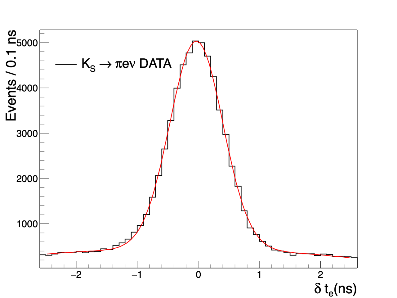
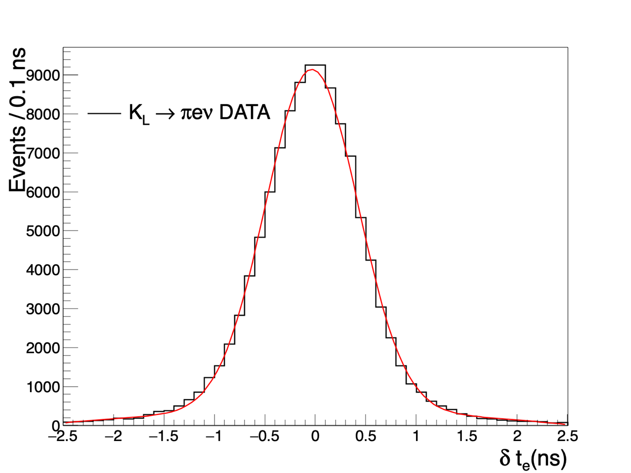
Figure 8: Comparison of the $\delta t_{e}$ distribution for the signal (left) and for the $K_{L}\to\pi e\nu$ control sample (right).

The fit to the $m_{e}^{2}$ distribution in Figure 6 is repeated varying the range and the bin size. The fit is also done using two separate components for $K_{S}\to\pi\mu\nu$ and $\phi\to K^{+}K^{-}$, the $\chi^{2}$ is good but the statistical error is slightly increased. Half of the difference between maximum and minimum result of the different fits, $\pm 0.15\%$, is taken as relative systematic uncertainty. The systematic uncertainties are listed in Table 6.

Table 6: Absolute systematic uncertainties.

	Selection	$\delta\epsilon_{\pi e\nu}^{\rm syst}$ [ $10^{-4}$ ]	$\delta\epsilon_{\pi^{+}\pi^{-}}^{\rm syst}$ [ $10^{-4}$ ]
	BDT selection	5.3
$K_{S}\to\pi e\nu$	TCA & TOF selection	6.0
	Fit parameters	3.0
$K_{S}\to\pi^{+}\pi^{-}$	Event selection		8.8
	Total	8.5	8.8

The dependence of $R_{\epsilon}$ on systematic effects has been studied in previous analyses for different $K_{S}$ decays selected with the $K_{L}$–crash tagging method: $K_{S}\to\pi^{+}\pi^{-}$ and $K_{S}\to\pi^{0}\pi^{0}$ ref:KStopipi , and $K_{S}\to\pi e\nu$ ref:KStopienuAsimmetry . The systematic uncertainties are evaluated by a comparison of data with simulation, the difference from one of the ratio $\frac{{\rm Data}}{{\rm MC}}$ is taken as systematic uncertainty.

Trigger – Two triggers are used for recording the events, the calorimeter trigger and the drift chamber trigger. The validation of the MC relative efficiency is derived from the comparison of the single-trigger and coincidence rates with the data. The data over MC ratio is 0.999 with negligible error.

On-line filter – The on-line filter rejects events triggered by beam background, detector noise, and events surviving the cosmic-ray veto. A fraction of non-filtered events prescaled by a factor of 20 allows to validate the MC efficiency of the filter. The data over MC ratio does not deviate from one by more than 0.1%.

Event classification – The event classification produces different streams for the analyses. The $K_{L}K_{S}$ stream used in this analysis selects events based on the properties of $K_{S}$ and $K_{L}$ decays. In more than 99% of the cases the events are selected based on the $K_{S}$ decay topology and the $K_{L}$–crash signature and differences between MC and data are accounted for in the systematic uncertainties described below for the $K_{L}$–crash and $K_{S}$ vertex reconstruction.

T₀ – The trigger time is synchronised with the r.f. signal and the event T₀ is re-defined after event reconstruction. The systematic uncertainty is evaluated analysing the data and MC distributions of T₀ for the decays with the most different timing properties: $K_{S}\to\pi^{+}\pi^{-}$ and $K_{S}\to\pi^{0}\pi^{0}$ ref:KStopipi . The data over MC ratio does not deviate from one by more than 0.1%.

$K_{L}$–crash and $\beta^{*}$ selection. – The systematic uncertainty is evaluated comparing data and simulated events tagged by $K_{S}\to\pi^{+}\pi^{-}$ and $K_{S}\to\pi^{0}\pi^{0}$ decays which have different timing and topology characteristics. The data over MC ratio is 1.001 with negligible error.

$K_{S}$ vertex reconstruction – The systematic uncertainty of the requirement of two tracks forming a vertex in the cylinder defined by Eq. (2) is evaluated for signal and normalisation using a control sample of $\phi\to\pi^{+}\pi^{0}\pi^{-}$ events selected requiring one track with minimum distance of approach to the beamline in the cylinder and a well-reconstructed $\pi^{0}$. Energy-momentum conservation determines the momentum of the second track. The momentum distribution of tracks in the control sample covers a range wider than both signal and normalisation samples. The efficiency for reconstructing the second track and the vertex is computed for data and simulation and the ratio $r(p_{\rm L},p_{\rm T})=\frac{\epsilon^{\rm Data}}{\epsilon^{\rm MC}}$ is parameterised as function of the longitudinal and transverse momentum $p_{\rm L}$ and $p_{\rm T}$. The ratios relative to the signal and normalisation events, $r_{\pi e\nu}$ and $r_{\pi^{+}\pi^{-}}$, are obtained as convolution of $r(p_{\rm L},p_{\rm T})$ with the respective momentum distribution after preselection. The ratio $\frac{r_{\pi^{+}\pi^{-}}}{r_{\pi e\nu}}$ deviates from one by $0.45\%$ with an uncertainty of 0.2% due to the knowledge of the parameters of the $r(p_{\rm L},p_{\rm T})$ function.

The $R_{\epsilon}$ total systematic uncertainty is estimated by combining the differences from one of the data over MC ratios and amounts to 0.48%. Including the systematic uncertainties the factors in Eq. (1) are:

$$\begin{array}[]{l}\epsilon_{\pi^{+}\pi^{-}}=(96.657\pm 0.088)\%,\\ \epsilon_{\pi e\nu}=(19.38\pm 0.10)\%,\\ {\rm and}\quad R_{\epsilon}=1.1882\pm 0.0059.\end{array}$$ (9)

5 The result

Using Eq. (1) with $N_{\pi e\nu}=49647\pm 316$, $N_{\pi\pi}=(282314\pm 17)\times 10^{3}$ events and the efficiencies of Eq. (9) we derive the ratio

$$\mathcal{R}=(1.0421\pm 0.0066_{\rm stat}\pm 0.0075_{\rm syst})\times 10^{-3}.$$

The previous result from KLOE based on an independent data sample corresponding to an integrated luminosity of 0.41 fb^-1 is $\mathcal{R}=(1.019\pm 0.011_{\rm stat}\pm 0.007_{\rm syst})\times 10^{-3}$ ref:KStopienu . Correlations exist between the two measurements in the determination of efficiencies for the event preselection and time-of-flight analysis, correlations in the determination of $R_{\epsilon}$ and the fit being negligible. The correlation coefficient is 12%. The combination of the two measurements gives

$$\mathcal{R}=\frac{\Gamma(K_{S}\to\pi e\nu)}{\Gamma(K_{S}\to\pi^{+}\pi^{-})}=(1.0338\pm 0.0054_{\rm stat}\pm 0.0064_{\rm syst})\times 10^{-3}.$$

Using the value $\mathcal{B}(K_{S}\to\pi^{+}\pi^{-})=0.69196\pm 0.00051$ measured by KLOE ref:KStopipi , we derive the branching fraction

$$\mathcal{B}(K_{S}\to\pi e\nu)=(7.153\pm 0.037_{\rm stat}\pm 0.044_{\rm syst})\times 10^{-4}=(7.153\pm 0.058)\times 10^{-4}.$$

The value of $|V_{us}|$ is related to the $K_{S}$ semileptonic branching fraction by the equation

$$\mathcal{B}(K_{S}\to\pi\ell\nu)=\frac{G^{2}(f_{+}(0)|V_{us}|)^{2}}{192\pi^{3}}\tau_{S}m_{K}^{5}I^{\ell}_{K}S_{\rm EW}(1+\delta^{K\ell}_{\rm EM}),$$

where $I^{\ell}_{K}$ is the phase-space integral, which depends on measured semileptonic form factors, $S_{\rm EW}$ is the short-distance electro-weak correction, $\delta^{K\ell}_{\rm EM}$ is the mode-dependent long-distance radiative correction, and $f_{+}(0)$ is the form factor at zero momentum transfer for the $\ell\nu$ system. Using the values $S_{\rm EW}=1.0232\pm 0.0003$ ref:Sirlin1993 , $I^{e}_{K}=0.15470\pm 0.00015$ and $\delta^{Ke}_{\rm EM}=(1.16\pm 0.03)\ 10^{-2}$ from Ref. ref:VusUpdate , and the world average values for the $K_{S}$ mass and lifetime ref:PDG we derive

$$f_{+}(0)|V_{us}|=0.2170\pm 0.0009.$$

6 Conclusion

A measurement of the ratio $\mathcal{R}=\Gamma(K_{S}\to\pi e\nu)/\Gamma(K_{S}\to\pi^{+}\pi^{-})$ is presented based on data collected with the KLOE experiment at the DA$\Phi$NE $\phi$-factory corresponding to an integrated luminosity of 1.63 fb^-1. The $\phi\to K_{L}K_{S}$ decays are exploited to select samples of pure and quasi-monochromatic $K_{S}$ mesons and data control samples of $K_{L}\to\pi e\nu$ decays. The $K_{S}$ decays are tagged by the detection of a $K_{L}$ interaction in the detector. The $K_{S}\to\pi e\nu$ events are selected by a boosted decision tree built with kinematic variables and by measurements of time-of-flight. The efficiencies for detecting the $K_{S}\to\pi e\nu$ decays are derived from $K_{L}\to\pi e\nu$ data control samples. A fit to the $m^{2}$ distribution of the identified electron track finds $49647\pm 316$ signal events. Normalising to $K_{S}\to\pi^{+}\pi^{-}$ decay events recorded in the same dataset, the result is $\mathcal{R}=(1.0421\pm 0.0066_{\rm stat}\pm 0.0075_{\rm syst})\times 10^{-3}$. The combination with our previous measurement gives $\mathcal{R}=(1.0338\pm 0.0054_{\rm stat}\pm 0.0064_{\rm syst})\times 10^{-3}$. From this value we derive the branching fraction $\mathcal{B}(K_{S}\to\pi e\nu)=(7.153\pm 0.037_{\rm stat}\pm 0.044_{\rm syst})\times 10^{-4}$ and the value of $|V_{us}|$ times the form factor at zero momentum transfer, $f_{+}(0)|V_{us}|=0.2170\pm 0.009$.

- (1) Y. Grossman, E. Passemar and S. Schachta, On the statistical treatment of the Cabibbo angle anomaly, JHEP 07 (2020) 068, arXiv:1911.07821 [hep-ph].
- (2) M. Antonelli et al., An evaluation of and precise tests of the Standard Model from world data on leptonic and semileptonic kaon decays, Eur. Phys. J. C 69 (2010) 399, arXiv:1005.2323 [hep-ph].
- (3) M. Moulson and E. Passemar, Status of determination for kaon decays, 10th International Workshop on the CKM Unitarity Triangle, University of Heidelberg, Germany, September 17-21, 2018, DOI:10.5281/zenodo.2565479.
- (4) E. Blucher and W.J. Marciano, , , the Cabibbo angle, and CKM unitarity, in The Review of Particle Physics, P.A. Zyla et al. (Particle Data Group), Prog. Theor. Exp. Phys. 2020 (2020) 083C01.
- (5) C.-Y. Seng, D. Galviz, W.J. Marciano, and U.-G. Meissner, Update on and from semileptonic kaon and pion decays, Phys. Rev. D 105 (2022) 013005, arXiv:2107.14708 [hep-ph].
- (6) R.R. Akhmetshin et al., Observation of semileptonic decays with the CMD-2 detector, Phys. Lett. B 456 (1999) 90, arXiv:hep-ex/9905022.
- (7) A. Aloisio et al., Measurement of the branching fraction for the decay , Phys. Lett. B 535 (2002) 37, arXiv:hep-ph/0203232.
- (8) D. Babusci et al., Measurement of the branching fraction for the decay with the KLOE detector, Phys. Lett. B 805 (2020) 135378, arXiv:1912.05990 [hep-ex].
- (9) J.R. Batley et al., Determination of the relative decay rate , Phys. Lett. B 653 (2007) 145.
- (10) F. Ambrosino et al., Study of the branching ratio and charge asymmetry for the decay with the KLOE detector, Phys. Lett. B 636 (2006) 173, arXiv:hep-ex/0601026.
- (11) A. Gallo et al., DANE Status Report, European Particle Accelerator Conference, 26-30 June 2006, Edinburgh, Scotland, Conf. Proc. C060626 (2006) 604.
- (12) F. Ambrosino et al., Measurement of the DANE luminosity with the KLOE detector using large angle Bhabha scattering, Eur. Phys. J. C 47 (2006) 589, arXiv:hep-ex/0604048.
- (13) F. Ambrosino et al., Precise measurement of , with the KLOE detector at DANE, Eur. Phys. J. C 48 (2006) 767, arXiv:hep-ex/0601025.
- (14) M. Adinolfi et al., The QCAL tile calorimeter of KLOE, Nucl. Instrum. Meth. A 483 (2002) 649.
- (15) M. Adinolfi et al., The tracking detector of the KLOE experiment, Nucl. Instrum. Meth. A 488 (2002) 51.
- (16) M. Adinolfi et al., The KLOE electromagnetic calorimeter, Nucl. Instrum. Meth. A 482 (2002) 364.
- (17) M. Adinolfi et al., The trigger system of the KLOE experiment, Nucl. Instrum. Meth. A 492 (2002) 134.
- (18) F. Ambrosino et al., Data handling, reconstruction and simulation for the KLOE experiment, Nucl. Instrum. Meth. A 534 (2004) 403, arXiv:physics/0404100.
- (19) A. Anastasi et al., Measurement of the charge asymmetry for the decay and test of CPT symmetry with the KLOE detector, JHEP 09 (2018) 021, arXiv:1806.08654 [hep-ex].
- (20) F. Ambrosino et al., Measurements of the absolute branching ratios for the dominant decays, the lifetime and with the KLOE detector, Phys. Lett. B 632 (2006) 43, arXiv:hep-ex/0509045.
- (21) W.J. Marciano and A. Sirlin, Radiative Corrections to Decays, Phys. Rev. Lett. 71 (1993) 3629.
- (22) The Review of Particle Physics, P. A. Zyla et al. (Particle Data Group), Prog. Theor. Exp. Phys. 2020 (2020) 083C01.
- (23) M. Zobov et al., Test of crab-waist collisions at the DANE factory, Phys. Rev. Lett. 104 (2010) 174801.
- (24) C. Milardi et al., High luminosity interaction region design for collisions inside high field detector solenoid, JINST 7 (2012) T03002.