Evolving finite elements for advection diffusion with an evolving interface

Abstract.

The aim of this paper is to develop a numerical scheme to approximate evolving interface problems for parabolic equations based on the abstract evolving finite element framework proposed in [23]. An appropriate weak formulation of the problem is derived for the use of evolving finite elements designed to accommodate for a moving interface. Optimal order error bounds are proved for arbitrary order evolving isoparametric finite elements. The paper concludes with numerical results for a model problem verifying orders of convergence.

1. Introduction

The model studied in the paper is the following, let $\Omega$ be a stationary domain with a moving interface $\Gamma(t)$ that encloses a subdomain $\Omega_{1}(t)$ and let $\Omega_{2}(t)=\Omega\setminus\overline{\Omega}_{1}(t)$. We denote by $\nu_{\Gamma}$ the outward pointing normal to $\Omega_{1}(t)$. Let, for $i=1$ and $2$, $\mathcal{A}_{i}$ be a diffusion tensor field, $\mathcal{B}_{i}$ be a vector field and $\mathcal{C}_{i}$ be a scalar field, each continuous on $\Omega_{i}(t)$. Let $f_{1},f_{2}$ and $g$ be time-dependent functions on $\Omega_{1}(t)$, $\Omega_{2}(t)$ and $\Gamma(t)$ respectively. More precise definitions of the problem data are given in Thm. 2.16. We are interested in well posedness and a suitable finite element scheme for the solutions of the following problem: Find scalar fields $u_{1}$ on the subdomain $\Omega_{1}(t)$ and $u_{2}$ on the subdomain $\Omega_{2}(t)$, which satisfy:

$$\partial_{t}u_{i}-\nabla\cdot(\mathcal{A}_{i}(t;x)\nabla u_{i})+\mathcal{B}_{i}(t;x)\cdot\nabla u_{i}+\mathcal{C}_{i}(t;x)u_{i} =f_{i}(t;x) \quad\text{in}\;\Omega_{i}(t),$$ (1.1a)

$$u_{2} =0 \quad\text{on}\;\partial\Omega,$$ (1.1b)

$$u_{1}-u_{2} =0 \quad\text{on}\;\Gamma(t),$$ (1.1c)

$$\mathcal{A}_{1}(t;x)\frac{\partial}{\partial\nu_{\Gamma}}u_{1}\bigg{|}_{\Gamma(t)}-\mathcal{A}_{2}(t;x)\frac{\partial}{\partial\nu_{\Gamma}}u_{2}\bigg{|}_{\Gamma(t)} =g(t;x) \quad\text{on}\;\Gamma(t),$$ (1.1d)

$$u_{i}(0) =u_{i}^{0} \quad\text{on}\;\Omega_{i}(0).$$ (1.1e)

Such equations can arise as subproblems when modelling the transport and diffusion of the concentration of a dissolved chemical species in evolving spatial domains. In particular, we mention applications in fluid dynamics [50, 12, 2], materials science [11, 29] and cell biology [51, 48, 30].

There are two main difficulties concerning this problem. The first of which is the evolution of the sub-domains and the second is the presence of a discontinuous jump across the interface. One common approach to moving domains is the ALE (Arbitrary Eulerian Lagrangian) method, see [33, 49, 39]. This involves having a parametrisation of the evolving region. The flow associated with this parametrisation could be physical or could be made to fit a specific purpose such as in [19] where the flow is chosen using knowledge of the surface velocity to construct a harmonic extension. Another common method is to use a discontinuous or immersed Galerkin method [52, 3, 41]. In this paper we propose and analyse an ALE approach using evolving finite elements on an evolving fitted mesh allowing the use of isoparametric elements that accurately approximate the boundary and result in higher order error estimates. The underlying parametrisation is assumed given.

The key contributions of this work are:

• We provide a functional analytic setting to show well posedness of the continuous problem, 1.1.

• We provide an ALE approach based on evolving isoparametric finite element spaces attached to evolving sub-domains. The evolving mesh is based on moving the Lagrange nodes with a given known smooth velocity. Achieving a higher order method requires a good initial mesh.

• We provide a robust error bound which demonstrates the error in an $L^{2}$ norm is bounded, up to a constant, by $h^{k+1}$, where $h$ represents the mesh size and $k$ is the degree of polynomials used both for the discretisation of the domain and the solution. This is the same order error as if we interpolated a known smooth solution.

• Numerical results and the simulation code are provided both to demonstrate the results and to allow others to use the implementation.

The assumption is made that we are given a global, smooth velocity field $\mathbf{w}$. Furthermore, the velocity field is such that moving the nodes of the mesh with the $\mathbf{w}$ preserves the regularity of the mesh over time. The velocity may be derived from physical considerations or otherwise an arbitrary velocity constructed in order to define a well behaved numerical scheme. We do not address how to achieve such a velocity in this work. There are methods in the literature to prevent mesh deformation, which involve re-parametrising the flow responsible for the movement of the interface into a more suitable flow, see, for example, [10, 20, 21].

1.1. Outline

Sec. 2 gives a well posedness analysis of the continuous equations along with the necessary functional analysis setting. The finite element construction is in Sec. 3 and the finite element scheme is in Sec. 4. An optimal order error bound is shown in Sec. 5 under smoothness assumptions on the domain and its evolution and the solution. Sec. 6 includes a time discretisation of the finite element scheme along with numerical experiences demonstrating the error bounds are tight. The Appendix includes further details of the proof the well posedness of the continuous scheme.

2. Evolving space formulation and well posedness

In this paper, $c$ will be used as a generic constant that depends on no quantity of particular importance. We use $(\cdot,\cdot)_{H}$ for an inner product on a Hilbert space $H$ and $\langle\cdot,\cdot\rangle_{X}$ as the dual pairing between a Banach space $X$ and its topological dual $X^{\prime}$.

2.1. Evolving Hilbert Spaces

We set up the necessary tools from the theory of evolving Sobolev spaces which were introduced and developed in [5, 6, 4]. We will only concern ourselves with the Hilbert case. A more general theory is developed in [4] concerning general Banach spaces. Let $I=[0,T]$ be a closed time interval and let $\{X(t)\}_{t\in I}$ be a family of Hilbert spaces equipped with norm $\|\cdot\|_{X(t)}$. Assume that there exists a linear map $\phi_{t}:X(0)\to X(t)$ satisfying the following properties:

1. The map $\phi_{t}$ is invertible for all $t\in I$ with inverse denoted by $\phi_{-t}$ and $\phi_{0}$ being the identity.

2. There exists a constant $C$ independent of time such that $\|\phi_{t}\eta\|_{X(t)}\leq C\|\eta\|_{X(0)}$, $\|\phi_{-t}\widetilde{\eta}\|_{X(0)}\leq C\|\widetilde{\eta}\|_{X(t)}$, for all $\eta\in X(0)$ and $\widetilde{\eta}\in X(t)$, for all $t\in I$.

3. The map $t\mapsto\|\phi_{t}\eta\|_{X(t)}$ is measurable for all $\eta\in X(0)$.

Here and elsewhere we use the notation $\phi_{t}\eta$ to denote the map $\phi_{t}$ applied to $\eta$. If such a map $\phi_{t}$ exists then we call it the flow map and the pair $(X(t),\phi_{t})_{t\in I}$ a compatible pair. Given a compatible pair, define the Hilbert moving spaces as:

$$L^{2}_{X}: =\bigg{\{}\eta:I\to\bigcup_{t\in I}X(t)\times\{t\},\quad t\mapsto(\widehat{\eta}(t),t)\,|\,\phi_{-t}\widehat{\eta}(t)\in L^{2}(I;X(0))\bigg{\}},$$ (2.1)

and the uniformly bounded equivalent:

$$L^{\infty}_{X}: =\bigg{\{}\eta:I\to\bigcup_{t\in I}X(t)\times\{t\},\quad t\mapsto(\widehat{\eta}(t),t)\,|\,\phi_{-t}\widehat{\eta}(t)\in L^{\infty}(I;X(0))\bigg{\}}.$$ (2.2)

We identify $\eta(t)=(\widehat{\eta}(t),t)$ with $\widehat{\eta}(t)$. The spaces $L^{p}_{X}$ are equipped with the norm:

$$\|\eta\|_{L^{p}_{X}}:=\begin{cases}\left({\int_{0}^{T}\|\eta(t)\|_{X(t)}^{2}}\right)^{\frac{1}{2}}&\text{for }p=2,\\ \operatorname*{ess\,sup}_{t\in[0,T]}\|\eta(t)\|_{X(t)}&\text{for }p=\infty.\end{cases}$$

$L^{2}_{X}$ is indeed a Hilbert space, see [4, Thm. 3.4]. The analogues of the spaces of continuous functions and of compactly supported smooth functions are defined as:

$$C^{k}_{X} :=\bigg{\{}\eta:I\to\bigcup_{t\in I}X(t)\times\{t\},\quad t\to(\widehat{\eta}(t),t)\,|\,\phi_{-t}\widehat{\eta}(t)\in C^{k}(I;X(0))\bigg{\}},$$

$$\mathcal{D}_{X} :=\bigg{\{}\eta:I\to\bigcup_{t\in I}X(t)\times\{t\},\quad t\to(\widehat{\eta}(t),t)\,|\,\phi_{-t}\widehat{\eta}(t)\in\mathcal{D}(I;X(0))\bigg{\}}.$$

Remark 2.1.

1. The use of a Cartesian product $\times$ inside the union in 2.1 rather then just taking the union of $\{X(t)\}_{t\in I}$ by itself is in order to guarantee a disjoint union which is crucial to identify the function point-wise.

2. Note that the spaces $L^{p}_{X}$ do not depend on the choice of the map $\phi_{t}$.

The strong material derivative in the evolving Hilbert space setting is defined as follows:

$$\partial_{t}^{\bullet}\eta:=\phi_{t}\partial_{t}(\phi_{-t}\eta),\quad\eta\in C^{1}_{X}.$$

Lemma 2.2 ([4], Thm. 2.4).

Given a compatible pair $(X(t),\phi_{t})_{t\in I}$, the maps $\phi_{t}:L^{2}(I;X(0))\to L^{2}_{X}$ and $\phi_{-t}:L^{2}_{X}\to L^{2}(I;X(0))$ define continuous linear isomorphism to their respective spaces.

Now assume $\{X(t)\}_{t\in I}$, $\{Y(t)\}_{t\in I}$ and $\{X^{*}(t)\}_{t\in I}$ are families of Hilbert spaces, with $X^{*}(t)$ the dual of $X(t)$ for all $t\in I$ (crucially, $X(t)$ and $X^{*}(t)$ are not identified). Assume further that for all $t\in I$, $X(t)\subset Y(t)\cong Y^{*}(t)\subset X^{*}(t)$ constitutes a Hilbert triple (in the sense that $X(t)$ is densely and continuously embedded into $Y(t)$ and $Y(t)$ is identified with its dual via Riesz representation). It is also assumed that there exists a map $\phi_{t}:Y(0)\to Y(t)$ with $\phi_{t}|_{X(0)}:X(0)\to X(t)$ with adjoint flow $\phi_{-t}^{*}:X^{*}(0)\to X^{*}(t)$,

$$\langle\phi_{-t}^{*}f,v\rangle_{X(t)}:=\langle f,\phi_{-t}v\rangle_{X(0)},\quad f\in X^{*}(0),\,v\in X(t),$$

such that $(X(t),\phi_{t}|_{X(t)})_{t\in I}$, $(Y(t),\phi_{t})_{t\in I}$ and $(X^{*}(t),\phi_{-t}^{*})_{t\in I}$ all define compatible pairs and therefore we can define the spaces $L^{2}_{X},\;L^{2}_{Y},\;L^{2}_{X^{*}}$ with their respective flows. In this case, just as for Bochner spaces, we have the have that $(L^{2}_{X})^{*}$ is isometrically isomorphic to $L^{2}_{X^{*}}$ [4, Thm. 3.7]. Moreover, the Hilbert triple structure is preserved: $L^{2}_{X}\subset L^{2}_{Y}\subset L^{2}_{X^{*}}$. Note that $L^{2}_{Y}$ remains a Hilbert space with a natural inner product structure, see [4, Rem. 3.9]. In order to generalise the concept of a “weak time derivative” to the evolving space, we first assume the following:

1. The map $t\mapsto\langle\phi_{t}w_{0},\phi_{t}v_{0}\rangle_{X(t)}=(\phi_{t}w_{0},\phi_{t}v_{0})_{Y(t)}$ is continuously differentiable for fixed $w_{0},v_{0}\in X_{0}$.

2. For all $t\in I$, the map:

   $$[w_{0},v_{0}]\mapsto\frac{d}{dt}(\phi_{t}w_{0},\phi_{t}v_{0})_{Y(t)},$$

   for $[w_{0},v_{0}]\in X(0)\times X(0)$ is continuous.

3. There exists a constant $C_{\lambda}$ independent of time such that, for almost all $t\in I$ and $w_{0},v_{0}\in X(0)$, we have:

   $$\bigg{|}\frac{d}{dt}(\phi_{t}w_{0},\phi_{t}v_{0})_{Y(t)}\bigg{|}\leq C_{\lambda}\|w_{0}\|_{Y(0)}\|v_{0}\|_{Y(0)}.$$

Definition 2.3.

Let Ass. $D1$ to $D3$ hold and label:

$$\lambda(t;w,v):=\bigg{[}\frac{d}{dt}(\phi_{t}w_{0},\phi_{t}v_{0})_{Y(t)}\bigg{]}\bigg{|}_{(w_{0},v_{0})=(\phi_{-t}w,\phi_{-t}v)},\quad w,v\in X(t).$$

Then $\lambda(t;\cdot,\cdot):Y(t)\times Y(t)\to\mathbb{R}$ is a continuous, symmetric, bounded and bilinear for almost all $t\in I$. We say $w\in L^{1}_{X}$ has a weak material derivative if there exists $v\in L^{1}_{X^{*}}$ such that:

$$\int_{0}^{T}(w(t),\partial^{\bullet}_{t}\eta)_{Y(t)}\,dt=\int_{0}^{T}\langle v(t),\eta\rangle_{X(t)}+\lambda(t;w,\eta)\,dt,$$

for all $\eta\in\mathcal{D}_{X}$. We label the weak material derivative $v=\partial_{t}^{\bullet}w$.

This definition follows all properties we expect from a weak derivative, such as being equivalent to the strong material derivative if the function is regular enough.

This allows us to define the equivalent of the Bochner solution space.

Definition 2.4.

We define $W(X,Y):=\left\{v\in L^{2}_{X},\;\partial_{t}^{\bullet}v\in L^{2}_{Y}\right\}$ with the norm:

$$\|v\|^{2}_{W(X,Y)}:=\|v\|^{2}_{L^{2}_{X}}+\|\partial_{t}^{\bullet}v\|^{2}_{L^{2}_{Y}}$$

and the solution space $W(X,X^{*}):=\left\{v\in L^{2}_{X},\;\partial_{t}^{\bullet}v\in L^{2}_{X^{*}}\right\}$ with the norm:

$$\|v\|^{2}_{W}:=\|v\|^{2}_{L^{2}_{X}}+\|\partial_{t}^{\bullet}v\|^{2}_{L^{2}_{X^{*}}}.$$

Definition 2.5.

The space $W(X,Y)$ is said to satisfy moving space equivalence if:

$$v\in W(X,Y)\iff\phi_{-t}v\in\mathcal{W}^{2,2}(X(0),Y(0)),$$

where $\mathcal{W}^{2,2}(X(0),Y(0))=\{v_{0}\in L^{2}(I;X(0)),\;\partial_{t}v\in L^{2}(I;Y(0))\}.$

Theorem 2.6 (The Transport Theorem).

Assume $v,w\in W(X,X^{*})$ and the moving space equivalence is satisfied, then, the map $t\mapsto(v,w)_{Y(t)}$ is uniformly continuous and for almost all $t\in I$, and the following holds:

$$\frac{d}{dt}(v,w)_{Y(t)}=\langle\partial_{t}^{\bullet}v,w\rangle_{X(t)}+\langle\partial_{t}^{\bullet}w,v\rangle_{X(t)}+\lambda(t;u,v).$$

Moreover, $C^{0}_{Y}\hookrightarrow W(X,X^{*})$.

See [4, Sec. 4.5] for proofs.

Lemma 2.7 (Characterisation of Material Derivative).

Let the moving space equivalence hold for $W(X,X)$, then for $v\in W(X,X)$, we have $v\in C_{X}^{0}$ and there exists a function $v_{0}\in\mathcal{W}^{2,2}(X(0),X(0))$ such that $v=\phi_{t}v_{0}$. Moreover, $C^{1}_{X}$ is dense in $W(X,X)$.

This follows from [4, Lem. 3.20]. Importantly, this implies $\partial_{t}^{\bullet}v=0$ if and only if $v=\phi_{t}v_{0}$ for some $v_{0}\in X(0)$.

2.2. Setting up the Domain

                                       

Figure 2.1. An example configuration of the domain.

Let $\Omega$ be a stationary domain in $\mathbb{R}^{d}$, $d=2,3$, with piecewise linear boundary and let $\{\Gamma(t),\;t\in I\}$ be a family of closed compact connected $C^{2+k}$ ($k\geq 0$) hypersurfaces with $\Gamma(t)\subset\Omega$. Let $\Omega_{1}(t)$ be a domain in $\Omega$ without boundary $\partial\Omega_{1}(t)=\Gamma(t)$ for all $t\in I$. Let $\Omega_{2}(t):=\Omega\setminus\Omega_{1}(t)$ and assume that $\Gamma(t)\cap\partial\Omega=\varnothing$ for all $t\in I$, then:

$$\overline{\Omega}=\overline{\Omega}_{1}(t)\cup\overline{\Omega}_{2}(t),\;\overline{\Omega}_{1}(t)\cap\overline{\Omega}_{2}(t)=\Gamma(t),\,\partial\Omega_{2}(t)=\Gamma(t)\cup\partial\Omega.$$

A sketch of the domains is shown in Fig. 2.1.

Remark 2.8.

The assumption that the outer boundary is piecewise linear is made to avoid having to analyse perturbation of the domain for Dirichlet boundary conditions, however the presented method and analysis can easily be altered if one removes this assumption.

We label the outer normals of $\Omega_{1}(t)$ and $\Omega_{2}(t)$ by $\nu_{\Gamma(t)}$ and $\nu_{\partial\Omega_{2}(t)}$ respectively. Let:

$$\mathcal{Q}_{i}:=\bigcup_{t\in I}\Omega_{i}(t)\times\{t\},\;\mathcal{Q}:=\Omega\times I.$$

Furthermore, we assume there exists a given, global velocity field $\mathbf{w}$ transporting $\Omega_{1}(t)$ and $\Omega_{2}(t)$, i.e $\mathbf{w}\cdot\nu_{\Gamma(t)}|_{\Gamma(t)}=V_{\Gamma}$ where $V_{\Gamma}$ is the normal velocity of $\Gamma(t)$, $\mathbf{w}\cdot\nu_{\partial\Omega_{2}(t)}|_{\partial\Gamma(t)}=-V_{\Gamma}$ and $\mathbf{w}\cdot\nu_{\partial\Omega_{2}(t)}|_{\partial\Gamma}=0$. Throughout the paper this velocity is assumed to be of regularity $\mathbf{w}\in C(I;C(\overline{\Omega};\mathbb{R}^{d}))$ with $\mathbf{w}_{i}(t;\cdot)\in C^{2}(\overline{\Omega}_{i}(t);\mathbb{R}^{d})$. Let $\mathbf{\Phi}_{i}(t;x):\overline{\Omega}_{i}(0)\to\overline{\Omega}_{i}(t)$ be the solution to the ordinary differential equations:

$$\frac{d}{dt}\mathbf{\Phi}_{i}(t;x) =\mathbf{w}(t;\mathbf{\Phi}_{i}(t;x))\qquad x\in\Omega_{i}(0),$$ (2.3)

$$\mathbf{\Phi}_{i}(0;x) =x.$$

We assume the solution exists and is of regularity $\mathbf{\Phi}_{i}\in C^{1}(\overline{\mathcal{Q}}_{i};\mathbb{R}^{d})$ with $\mathbf{\Phi}_{i}(t;\cdot)\colon\overline{\Omega}_{i}(0)\to\overline{\Omega}_{i}(t)$ and $\mathbf{\Phi}_{i}(t;\cdot)\in C^{2}(\Omega_{i}(0);\mathbb{R}^{d})$, see [47, Thm. 1.45] and [31, Thm. II.1.1, Sec. V] for the necessary additional conditions. Furthermore, both $\mathbf{\Phi}_{i}(t;\cdot)$ are invertible diffeomorphisms for all $t\in I$ with $\mathrm{Im}(\mathbf{\Phi}_{i}(t;\cdot))=\Omega_{i}(t)$. We denote by $\Phi_{i}(-t,\cdot)$ the inverse of $\Phi_{i}(t,\cdot)$. Since we assumed $\mathbf{w}\in C(I;C(\overline{\Omega};\mathbb{R}^{d}))$, it follows that $\mathbf{\Phi}_{1}(t;x)|_{\Gamma(0)}=\mathbf{\Phi}_{2}(t;x)|_{\Gamma(0)}$.

Remark 2.9.

For the abstract formulation of the problem, it is only required to assume that the velocity field $\mathbf{w}$ is of sufficient regularity. However, for the purpose of evolving the mesh later, we will assume this velocity field is known explicitly.

Let $J^{t}_{i}$ denote the determinant of Jacobian matrix, $J^{t}_{i}=\text{det}[\nabla\mathbf{\Phi}_{i}(t;x)]$. The prior assumptions imply $J^{t}_{i}(\cdot)\in C^{1}(\overline{\Omega}_{i}(0);\mathbb{R})$ and there exists $C_{\Omega}$ independent of time and space such that:

$$\frac{1}{C_{\Omega}}\leq|J_{i}^{t}|\leq C_{\Omega},$$

and $J^{-t}_{i}$ denotes its inverse.

Remark 2.10.

Note that we have assumed the global parametric velocity $\mathbf{w}$ is given. The solution of the partial differential equation system is independent of $\mathbf{w}$ apart from the requirements that $\mathbf{w}_{\Gamma}\cdot\nu_{\Gamma(t)}=V_{\Gamma}$ and $\mathbf{w}\cdot\nu_{\partial\Omega}=0$. However the evolving mesh does depend on $\mathbf{w}$ hence the discrete solution depends on the full parametric velocity.

Let $d_{\Gamma}(t;x)$ be the signed distance function to $\Gamma(t)$:

$$d_{\Gamma}(t;x)=\begin{cases}-\inf\{|x-y|:y\in\Gamma(t)\},\quad&\text{for}\,x\in\overline{\Omega}_{1}(t),\\ \inf\{|x-y|:y\in\Gamma(t)\},\quad&\text{for}\,x\in\Omega_{2}(t).\end{cases}$$

Then, since the interface is of class $C^{2}$, there exists a constant $\delta>0$ such that if $x\in\mathcal{N}_{\Gamma(t)}:=\{x\in\Omega.\;|d_{\Gamma}(t;x)|\leq\delta\}$, it can be uniquely decomposed as:

$$x=d_{\Gamma}(t;x)\nu_{\Gamma(t)}(\Pi_{t}(x))+\Pi_{t}(x),$$ (2.4)

where $\Pi_{t}(\cdot)$ is the nearest point on $\Gamma(t)$, i.e, $\Pi_{t}(x):=\inf\{|y-x|:y\in\Gamma(t)\}$ (see [43, Sec. 2.3]). We refer to the set $\mathcal{N}_{\Gamma(t)}$ as the tubular neighbourhood of $\Gamma(t)$. Note that $\delta$ can be chosen independently of time by the fact that $I$ is compact. Moreover, via the assumption that $\Gamma(t)\cap\partial\Omega=0$ for all $t\in I$, $\delta$ can be chosen small enough such that $\mathcal{N}_{\Gamma(t)}\cap\partial\Omega=\varnothing$ for all $t\in I$.

For the error analysis, we require further regularity of the flow to yield the results collected in the following lemma.

Lemma 2.11.

Let $\Theta\in\mathbb{N}$. Assume further regularity on the flow map $\mathbf{\Phi}\in C^{2+\Theta}\left(I;C^{2+\Theta}\left(\overline{\Omega}_{i}(t);\mathbb{R}^{d}\right)\right)$ and the initial surface $\Gamma(0)$ is class $C^{2+\Theta}$, then the following geometric quantity have additional regularity:

• $\Gamma(t)$ is of class $C^{2+\Theta}$,

• $J^{t}_{i}(\cdot)\in C^{1+\Theta}(\overline{\Omega}_{i}(0);\mathbb{R})$,

• $d_{\Gamma}(t;\cdot)\in C^{2+\Theta}(\mathcal{N}_{\Gamma(t)};\mathbb{R})$,

• $\Pi_{t}(\cdot)\in C^{1+\Theta}(\mathcal{N}_{\Gamma(t)};\mathbb{R}^{d})$.

See [25] and [27, Lem. 14.16].

2.3. Realisation

For a given function $v$ acting on $\Omega$, we decompose it as:

$$v_{1}:=v\chi_{\overline{\Omega}_{1}(t)},\quad v_{2}:=v\chi_{\overline{\Omega}_{2}(t)},$$

where $\chi_{\overline{\Omega}_{i}(t)}=1$ if $x\in\overline{\Omega}_{i}(t)$ and zero otherwise. A function $v$ on $\Omega$ will be identified as the pair $v=(v_{1},v_{2})$. The jump operator $\llbracket\cdot\rrbracket_{\Gamma(t)}:C(\overline{\Omega}_{1}(t);\mathbb{R})\times C(\overline{\Omega}_{1}(t);\mathbb{R})\to C(\Gamma(t);\mathbb{R})$ as:

$$\llbracket v\rrbracket_{\Gamma(t)}:=[v_{1}-v_{2}]|_{\Gamma(t)}.$$

This functional has a natural extension on the Cartesian product of standard Sobolev spaces $H^{1}(\Omega_{1}(t))\times H^{1}(\Omega_{2}(t))$ via use of the trace maps; $T_{i}(t):H^{1}(\Omega_{i}(t))\to H^{1/2}(\partial\Omega_{i}(t))$, $i\in\{1,2\}$, (see [46, Sec. 7.2.5] for an extensive definition of the trace map) as:

$$\llbracket v\rrbracket_{\Gamma(t)}:=[T_{1}(t)v_{1}-T_{2}(t)v_{2}]|_{\Gamma(t)}.$$

We define the following spaces:

$$H(t) :=L^{2}(\Omega_{1}(t))\times L^{2}(\Omega_{2}(t)),\quad\|v\|_{H(t)}^{2}:=\sum_{i=1}^{2}\|v_{i}\|^{2}_{L^{2}(\Omega_{i}(t))},$$

$$V(t) :=\{v\in H^{1}(\Omega_{1}(t))\times H^{1}(\Omega_{2}(t)),\,\llbracket v\rrbracket_{\Gamma(t)}=0,\;v_{2}|_{\partial\Omega}=0\},\quad\|v\|_{V(t)}^{2}:=\sum_{i=1}^{2}\|v_{i}\|^{2}_{H^{1}(\Omega_{i}(t))}$$

$$Z_{k}(t) :=\{w\in V(t)|\;w_{i}\in H^{1+k}(\Omega_{i}(t))\},\;\|w\|^{2}_{Z_{k}(t)}:=\sum_{i=1}^{2}\|w_{i}\|^{2}_{H^{1+k}(\Omega_{i}(t))}.$$

Note that due to the continuity of the trace operators $T_{i}(t)$ on $H^{1}(\Omega_{i}(t))$, $V(t)$ defines a closed subspace of $H^{1}(\Omega_{1}(t))\times H^{1}(\Omega_{2}(t))$ and contains $H_{0}^{1}(\Omega_{1}(t))\times H_{0}^{1}(\Omega_{2}(t))$, hence is dense within $H(t)$ . For an element $v=(v_{1},v_{2})\in V(t)$, we will identify $v|_{\Omega_{1}(t)}=v_{1}$ and $v|_{\Omega_{2}(t)}=v_{2}$. We also define the interface space:

$$H^{1/2}(\Gamma(t)) =\{v\in L^{2}(\Gamma(t)),\,|v|_{H^{1/2}(\Gamma(t))}<\infty\},\;|v|_{H^{1/2}(\Gamma(t))}:=\int_{\Gamma(t)}\int_{\Gamma(t)}\frac{|v(x)-v(y)|^{2}}{|x-y|^{d}}\,dxdy,$$

with norm given by:

$$\|v\|^{2}_{H^{1/2}(\Gamma(t))}: =\|v\|^{2}_{L^{2}(\Gamma(t))}+|v|^{2}_{H^{1/2}(\Gamma(t))}.$$

Then, $H^{1/2}(\Gamma(t))$ is a Hilbert space and moreover is dense and compactly embedded in $L^{2}(\Gamma(t))$ (see [40, Sec. 2]). For consistency of notation, let $\mathcal{V}_{\Gamma}(t)=H^{1/2}(\Gamma(t))$ and $\mathcal{H}_{\Gamma}(t)=L^{2}(\Gamma(t))$, and identify the Hilbert triple $\mathcal{V}_{\Gamma}(t)\subset\mathcal{H}_{\Gamma}(t)\subset\mathcal{V}_{\Gamma}^{*}(t)$.

Now for a function $v\in H(t)$ and $w\in\mathcal{H}_{\Gamma}(t)$, the respective flows are defined as:

$$\phi_{t}v:=(v_{1}(t;\mathbf{\Phi}_{1}(-t;x)),v_{2}(t;\mathbf{\Phi}_{2}(-t;x))),\quad\phi_{t}w:=w(t;\mathbf{\Phi}_{1}(-t;x)).$$

Lemma 2.12.

The pairs $(V(t),\phi_{t})|_{t\in I}$, $(H(t),\phi_{t})|_{t\in I}$, $(V^{*}(t),\phi_{-t}^{*})|_{t\in I}$, $(\mathcal{V}_{\Gamma}(t),\phi_{t})|_{t\in I}$, $(\mathcal{H}_{\Gamma}(t),\phi_{t})|_{t\in I}$ and $(\mathcal{V}_{\Gamma}^{*}(t),\phi_{-t}^{*})|_{t\in I}$ are all compatible.

Assuming the added regularity $\mathbf{\Phi}_{i}(t;\cdot)\in C^{1+k}(\Omega_{i}(0);\mathbb{R}^{d}))$, the pair $(Z_{k}(t),\phi_{t})|_{t\in I}$ is compatible.

Proof.

Ass. $B1$ to $B3$ need to be checked. This will be checked only for $V(t)$ as a similar logic can be employed for the remaining spaces. $B1$ follows from both $\mathbf{\Phi}_{1}(-t;x)$, $\mathbf{\Phi}_{2}(-t;x)$ being invertible diffeomorphisms. For $B2$, via simple manipulation:

$$\|\phi_{t}v\|^{2}_{V(t)} =\sum_{i=1}^{2}\int_{\Omega_{i}(t)}|v_{i}(t;\mathbf{\Phi}_{i}(-t;x))|^{2}+|\nabla v_{i}(t;\mathbf{\Phi}_{i}(-t;x))|^{2},$$

$$=\sum_{i=1}^{2}\int_{\Omega_{i}(0)}[\,|v_{i}(t;x)|^{2}+|[\nabla\mathbf{\Phi}_{i}(-t;y)]^{T}|_{y=\mathbf{\Phi}(t;x)}\nabla v_{i}(t;x)|^{2}]J^{t}_{i}$$ (2.5)

$$\leq c(|J^{t}_{i}|_{L^{\infty}(\Omega_{i}(0))},|\nabla\mathbf{\Phi}_{i}(-t,x)|_{L^{\infty}(\Omega_{i}(t))})\|v\|^{2}_{V(0)},$$

The bound follows from the assumption on the regularity of the velocity field. The same method shows a similar bound for $\|\phi_{-t}\widetilde{v}\|_{V(0)}\leq c\|\widetilde{v}\|_{V(t)}$ for all $\widetilde{v}\in V(t)$. To show measurability, $B3$, note that the second equality in Sec. 2.3 is continuous. For the compatibility of the boundary spaces $\mathcal{V}_{\Gamma}(t)$, $\mathcal{H}_{\Gamma}(t)$ and $\mathcal{V}^{*}_{\Gamma}(t)$, see [6, Sec. 4 and 5]. Under the added regularity the compatibility of $(Z_{k}(t),\phi_{t})|_{t\in I}$ follows similarly. ∎

We will identify both $V(t)\subset H(t)\subset V^{*}(t)$ and $\mathcal{V}_{\Gamma}(t)\subset\mathcal{H}_{\Gamma}(t)\subset\mathcal{V}_{\Gamma}^{*}(t)$ with the structure $X(t)\subset Y(t)\subset X^{*}(t)$ developed in Sec. 2.1.

Lemma 2.13.

The moving space equivalence is satisfied between $W(V,V^{*})$ and $\mathcal{W}(V(0),V^{*}(0))$.

Proof.

The proof follows similarly from the one given for [4, Prop. 7.4] as by assumption the Jacobian determinate is at least of regularity $J^{t}_{i}\in C^{1}(I;C^{1}(\overline{\Omega}_{i}(0);\mathbb{R}))$. ∎

Remark 2.14.

It does not matter which of the flows $\mathbf{\Phi}_{i}(t;x)$ is used to define $\mathcal{H}_{\Gamma}(t)$ as $\mathbf{\Phi}_{1}(t;x)|_{\Gamma(0)}=\mathbf{\Phi}_{2}(t;x)|_{\Gamma(0)}$. Moreover, it can be shown that $v=(v_{1},v_{2})\in V(t)$ if, and only if, $v_{1}\chi_{\Omega_{1}(t)}+v_{2}(1-\chi_{\Omega_{1}(t)})\in H^{1}_{0}(\Omega)$ with equivalent norms, hence the space $V(t)$ can be thought as an identification of the components of a functions in $H^{1}_{0}(\Omega)$.

We may define both moving space triples $L^{2}_{V}\subset L^{2}_{H}\subset L^{2}_{V^{*}}$ and $L^{2}_{\mathcal{V}_{\Gamma}}\subset L^{2}_{\mathcal{H}_{\Gamma}}\subset L^{2}_{\mathcal{V}^{*}_{\Gamma}}$.

Theorem 2.15 (Reynolds’ Transport Theorem).

Let $g_{i}\in C^{1}(\mathcal{Q}_{i};\mathbb{R})$, then:

$$\frac{d}{dt}\sum_{i=1}^{2}\int_{\Omega_{i}(t)}g_{i}=\sum_{i=1}^{2}\int_{\Omega_{i}(t)}\partial_{t}g_{i}+\mathbf{w}\cdot\nabla g_{i}+g_{i}\nabla\cdot\mathbf{w}.$$

Proof.

We use another version of Reynolds’ Transport Theorem given in [43, Sec. 2.5]. For $g=(g_{1},g_{2})\in C^{1}(\mathcal{Q}_{1};\mathbb{R})\times C^{1}(\mathcal{Q}_{2};\mathbb{R})$, then:

$$\frac{d}{dt}\int_{\Omega\setminus\Gamma(t)}g=\int_{\Omega\setminus\Gamma(t)}\partial_{t}g-\int_{\Gamma(t)}\llbracket g\rrbracket_{\Gamma(t)}V_{\Gamma}.$$

Note that here $\Omega\setminus\Gamma(t)=\Omega_{1}(t)\cup\Omega_{2}(t)$, and:

$$\sum_{i=1}^{2}\int_{\Omega_{i}(t)}\mathbf{w}\cdot\nabla g_{i}+g_{i}\nabla\cdot\mathbf{w}=\sum_{i=1}^{2}\int_{\Omega_{i}(t)}\nabla\cdot(\mathbf{w}g_{i}) =-\int_{\partial\Omega}[\mathbf{w}g_{i}]\cdot\nu_{\partial\Omega}-\int_{\Gamma(t)}\llbracket\mathbf{w}g\rrbracket_{\Gamma(t)}\cdot\nu_{\Gamma(t)},$$

$$=-\int_{\Gamma(t)}\llbracket g\rrbracket_{\Gamma(t)}V_{\Gamma}.\qed$$

Note that via use of the chain rule and the definition of $\mathbf{\Phi}(t;\cdot)$ 2.3, for a function $\eta_{i}\in C^{1}(\mathcal{Q}_{i};\mathbb{R})$:

$$\bigg{[}\frac{d}{dt}(\eta_{i}(t;\mathbf{\Phi}_{i}(t;x))\bigg{]}\bigg{|}_{x=\mathbf{\Phi}_{i}(-t;y)} =\partial_{t}\eta_{i}(t;y)+\partial_{t}(\mathbf{\Phi}_{i}(t;x))|_{x=\mathbf{\Phi}_{i}(-t;y)}\cdot\nabla\eta_{i}(t;x),$$

$$=\partial_{t}\eta_{i}(t;y)+\mathbf{w}(t;y)\cdot\nabla\eta_{i}(t;x).$$

Giving us back the classical definition for the material derivative, see [28, Sec 1.1.1]. For a function $v\in C^{1}_{V}$, we define:

$$\partial_{t}^{\bullet}v=\phi_{t}\frac{d}{dt}(v_{1}(t;\mathbf{\Phi}_{1}(t;x)),v_{2}(t;\mathbf{\Phi}_{2}(t;x)))=([\partial_{t}+\mathbf{w}\cdot\nabla]v_{1}(t;x),[\partial_{t}+\mathbf{w}\cdot\nabla]v_{2}(t;x))=:(\partial_{t}^{\bullet}v_{1},\partial_{t}^{\bullet}v_{2}).$$

One can check that due to the regularity of the flow, the assumptions $D1$ to $D3$ are satisfied on the triple $V(t)\subset H(t)\subset V^{*}(t)$, moreover, via Reynold’s transport theorem, one can check that the bilinear form $\lambda$ introduced Sec. 2.1 in this case becomes:

$$\lambda(t;v,\eta)=(\nabla\cdot\mathbf{w}v,\eta)_{H(t)}=\sum_{i=1}^{2}\int_{\Omega_{i}(t)}[\nabla\cdot\mathbf{w}]v_{i}\,\eta_{i}.$$ (2.6)

See [4, Lem. 6.3] for more details.

2.4. The Weak Formulation

Taking the strong problem 1.1, assuming there exists a regular enough solution $u$, we can rewrite the partial differential equation as:

$$\partial_{t}^{\bullet}u_{i}+\nabla\cdot\mathbf{w}u_{i}-\nabla\cdot(\mathcal{A}_{i}(t;x)\nabla u_{i})+[\mathcal{B}_{i}(t;x)-\mathbf{w}]\cdot\nabla u_{i}+[\mathcal{C}_{i}(t;x)-\nabla\cdot\mathbf{w}]u_{i}=f_{i}.$$ (2.7)

Here the term $\nabla\cdot\mathbf{w}$, corresponding to the previously identified bilinear form $\lambda(t;\cdot,\cdot)$, 2.6, is introduced to get the equation in a more convenient form. Then testing with a function $v\in L^{2}_{V}$ and using the interface condition, we arrive at the following variational problem:

$$\int_{0}^{T}\langle\partial_{t}^{\bullet}u,v\rangle_{V(t)}\,dt+\int_{0}^{T}\lambda(t;u,v)+\underbrace{\sum_{i=1}^{2}\int_{\Omega_{i}(t)}\mathcal{A}_{i}\nabla u_{i}\cdot\nabla v_{i}+[\mathcal{B}_{i}-\mathbf{w}]\cdot\nabla u_{i}\,v_{i}+[\mathcal{C}_{i}-\nabla\cdot\mathbf{w}]u_{i}\,v_{i}}_{=:a(t;u,v)}\,dt$$

$$=\int_{0}^{T}\underbrace{\langle f,v\rangle_{V(t)}+\langle g,v\rangle_{\mathcal{V}_{\Gamma}(t)}}_{=:l(t;v)}\,dt.$$

Note that here the Hilbert triple structure is used for the duality pairings; $\langle f,v\rangle_{V(t)}=(f,v)_{H(t)}$ and $\langle g,v\rangle_{\mathcal{V}_{\Gamma}(t)}=(g,v)_{\mathcal{H}_{\Gamma}(t)}$, and we have the initial condition $u(0)=u_{0}$. This gives us the weak formulation:

$$\int_{0}^{T}\langle\partial_{t}^{\bullet}u,v\rangle_{V(t)}+a(t;u,v)+\lambda(t;u,v)\,dt=\int_{0}^{T}l(t;v)\,dt,$$ (2.8)

for all $v\in L^{2}_{V}$. Moreover if, instead $v\in W(V,V^{*})$, we get the equivalent formulation via the transport theorem (for notational convenience later on, we will label the inner product $(\cdot,\cdot)_{H(t)}=:m(t;\cdot,\cdot)$):

$$\frac{d}{dt}m(t;u,v)+a(t;u,v)=m(t;u,\partial^{\bullet}_{t}v)+l(t;v).$$

If $\partial_{t}^{\bullet}u\in L^{2}_{H}$, then via identification of the Hilbert triple, we have:

$$\langle\partial_{t}^{\bullet}u,v\rangle_{V(t)}=m(t;\partial_{t}^{\bullet}u,v),$$

and the problem can be restated abstractly in this case as $u\in W(V,H)$ being the solution to:

$$m(t;\partial_{t}^{\bullet}u,v)+a(t;u,v)+\lambda(t;u,v)=l(t;v),$$ (2.9)

for almost all $t\in I$, and all $v\in L^{2}_{V}$.

2.5. Well Posedness

Theorem 2.16.

Assume the following:

1. The coefficients $\mathcal{A}_{i}\in C(\overline{\mathcal{Q}}_{i};\mathbb{R}^{d\times d})$, $\mathcal{B}_{i}\in C(\overline{\mathcal{Q}}_{i};\mathbb{R}^{d})$ and $\mathcal{C}_{i}\in C(\overline{\mathcal{Q}}_{i};\mathbb{R})$;

2. There exists a constant $\gamma>0$ such that:

   $$\inf_{t\in I}\inf_{x\in\Omega_{i}(t)}\mathcal{A}_{i}(t;x)\xi\cdot\xi^{T}\geq\gamma|\xi|^{2}\quad\forall\xi\in\mathbb{R}^{d};$$ (2.10)

3. $(u_{0},f,g,\mathbf{w}_{i},\mathbf{w})\in H(0)\times L^{2}_{V^{*}}\times L^{2}_{V_{\Gamma}^{*}}\times C^{1}(\overline{\mathcal{Q}}_{i},\mathbb{R}^{d})\times C(I\times\overline{\Omega};\mathbb{R}^{d}))$,

then there exists a unique solution $u\in W(V,V^{*})$ to 2.8 with inequality:

$$\|u\|_{W}\leq C\bigg{(}\|f\|_{L^{2}_{V^{*}}}+\|g\|_{L^{2}_{\mathcal{V}_{\Gamma}^{*}}}+\|u_{0}\|_{H(0)}\bigg{)}.$$

Furthermore, if it holds that:

1. $(u_{0},f,g,\mathcal{A}_{i})\in V(0)\times L^{2}_{H}\times W(\mathcal{V}_{\Gamma},\mathcal{V}^{*}_{\Gamma})\times C^{1}(\overline{\mathcal{Q}_{i}};\mathbb{R}^{d\times d})$, and $\mathcal{A}_{i}$ is symmetric,

then the solution is of additional regularity $u\in W(V,H)$ with bound:

$$\|u\|_{W(V,H)}\leq C\bigg{(}\|f\|_{L^{2}_{H}}+\|u_{0}\|_{V(0)}+\|g\|_{W(\mathcal{V}_{\Gamma},\mathcal{V}^{*}_{\Gamma})}\bigg{)}.$$

Proof.

The existence and uniqueness follows from a standard application of the Babuska-Lax-Milgram theorem in conjunction with Poincaré’s inequality, detailed in [5, Thm. 3.6]. The proof of additional regularity under Ass. $A4$ is given in the Appendix (Lem. A.4). ∎

Furthermore, in order to analyse the error in the finite element approximation of the material derivative, it is convenient to define notation for the derivative of the bilinear form $a(t;\cdot,\cdot)$ to be:

$$b(t;v,w):=\frac{d}{dt}[a(t;v,w)]-a(t;\partial^{\bullet}_{t}v,w)-a(t;v,\partial^{\bullet}_{t}w),\quad\forall v,w\in W(V,V).$$ (2.11)

Then, assuming furthermore that $\mathcal{A}_{i}\in C^{1}(\overline{\mathcal{Q}}_{i};\mathbb{R}^{d\times d})$, $\mathcal{B}_{i}\in C^{1}(\overline{\mathcal{Q}}_{i};\mathbb{R}^{d})$ and $\mathcal{C}_{i}\in C^{1}(\overline{\mathcal{Q}}_{i};\mathbb{R})$, the bilinear form $b(t;\cdot,\cdot)$ exists and can be explicitly calculated as:

$$b(t;v,w)=\sum_{i=1}^{2}\int_{\Omega_{i}(t)}\mathcal{D}^{\mathcal{A}}_{i}(\mathbf{w},\mathcal{A}_{i},v_{i},w_{i})+\mathcal{D}^{\mathcal{B}}_{i}(\mathbf{w},\mathcal{B}_{i},v_{i},w_{i})\\ \qquad\qquad\qquad\qquad+v_{i}\,w_{i}\partial^{\bullet}_{t}[\mathcal{C}_{i}-\nabla\cdot\mathbf{w}]+\nabla\cdot\mathbf{w}[\mathcal{C}_{i}-\nabla\cdot\mathbf{w}]v_{i}\,w_{i},$$ (2.12)

where

$$\mathcal{D}^{\mathcal{A}}_{i}(\mathbf{w},\mathcal{A}_{i},v_{i},w_{i}) =(\partial^{\bullet}_{t}\mathcal{A}_{i}(t;x)+\nabla\cdot\mathbf{w}\mathcal{A}_{i}(t;x))\nabla v_{i}\cdot\nabla w_{i}-2D_{i}(\mathbf{w},\mathcal{A}_{i})\nabla v_{i}\cdot\nabla w_{i},$$

$$\mathcal{D}^{\mathcal{B}}_{i}(\mathbf{w},\mathcal{B}_{i},v_{i},w_{i}) =\partial^{\bullet}_{t}[\mathcal{B}_{i}(t;x)-\mathbf{w}]\cdot\nabla v_{i}\,w_{i}+[\mathcal{B}_{i}(t;x)-\mathbf{w}]\cdot\nabla v_{i}\,w_{i}\nabla\cdot\mathbf{w}$$

$$\qquad\qquad-\sum_{j,k=1}^{d}[\mathcal{B}_{i}-\mathbf{w}]_{j}(\nabla_{j}\mathbf{w}_{k})\nabla_{k}v_{i}\,w_{i},$$

$$[D_{i}(\mathbf{w},\mathcal{A}_{i})]_{jl} =\frac{1}{2}\sum_{r=1}^{d}[\mathcal{A}_{i}(t;x)]_{jr}\nabla_{r}\mathbf{w}_{l}+[\mathcal{A}_{i}(t;x)]_{lr}\nabla_{r}\mathbf{w}_{j}.$$

Note that the derivative of the bilinear form $m(t;\cdot,\cdot)$ is already assumed to exist and equals $\lambda(t;\cdot,\cdot)$ introduced in Sec. 2.1.

3. Evolving finite elements

Figure 3.1. Showing the difference between a non viable initial mesh and an adequate one for a circle enclosed in a square. The one on the left breaking condition $M5$ whereas the one on the right following condition $M5$.

From this point on, we assume the additional geometric regularity as described in Lem. 2.11. We begin by detailing the initial triangulation of the domain and follow with the construction of the evolving mesh. In order to relate discrete and continuous functions we introduce the concept of a lift mapping and then finally define evolving finite element spaces.

3.1. Construction of the Initial Domain

Initial Mesh Construction/Assumption:

1. We first perform a partition into $d$-dimensional simplices corresponding to a polyhedral approximation $\widetilde{\Omega}^{h}_{1}$ of the interior domain $\overline{\Omega}_{1}(0)$, $\widetilde{\Omega}^{h}_{1}=\cup_{j=1}^{M_{1}}\widetilde{K}^{j}_{1}$, $\widetilde{\mathcal{J}}^{h}_{1}:=\{\widetilde{K}^{j}_{1}\}_{j=1}^{M_{1}}$, where $\widetilde{K}^{j}_{1}$ are the simplicial elements of positive diameter, bounded by some $\widetilde{h}$, and $M_{1}$ is the number of elements.

2. The set $\widetilde{\Omega}^{h}_{2}:=\overline{\Omega\setminus\widetilde{\Omega}^{h}_{1}}$ is polyhedral and we construct a partition into $d$-dimensional simplices $\widetilde{\mathcal{J}}^{h}_{1}:=\{\widetilde{K}^{j}_{2}\}_{j=1}^{M_{2}}$ with maximum diameter $\widetilde{h}$. Let $\widetilde{\mathcal{J}}^{h}=\cup_{i=1}^{2}\widetilde{\mathcal{J}}^{h}_{i}$ assume that all partitions $\{\widetilde{\mathcal{J}}_{1}^{h},\widetilde{\mathcal{J}}_{2}^{h},\widetilde{\mathcal{J}}^{h}\}$ are admissible, shape regular and quasi-uniform in $\{\widetilde{\Omega}_{1}^{h},\widetilde{\Omega}^{h}_{2},\overline{\Omega}\}$ respectively, see [13, Def. 5.1].

3. Each element $\widetilde{K}$ contains $d+1$ facets labelled $\{\widetilde{E}^{j}\}_{j=1}^{d+1}\subset\widetilde{K}$. We refer to the set of all facets of all elements in $\widetilde{\mathcal{J}}^{h}$ by $\widetilde{\mathcal{J}}^{h}_{\partial}$.

4. For $\widetilde{E}\in\widetilde{\mathcal{J}}^{h}_{\partial}$, if there exists $\widetilde{K}_{1}\in\widetilde{\mathcal{J}}_{1}^{h}$ and $\widetilde{K}_{2}\in\widetilde{\mathcal{J}}^{h}_{2}$ such that $\widetilde{E}=\widetilde{K}_{1}\cap\widetilde{K}_{2}$, then we call $\widetilde{E}$ an interface facet and label the collection of those facets $\widetilde{\mathcal{J}}_{\Gamma}^{h}$ and the union of interface facets $\widetilde{\Gamma}^{h}$. If for a given $\widetilde{E}$, there is only one element $\widetilde{K}\in\widetilde{\mathcal{J}}^{h}_{2}$ such that $\widetilde{E}\subset\widetilde{K}$, then such a facet is called a boundary facet.

5. We restrict the vertices of interface facets to be on $\Gamma(0)$, i.e, if $\widetilde{E}$ is an interface facet, and $\{\widetilde{a}_{\widetilde{E}}^{j}\}_{j=1}^{d-1}$ are the vertices of $\widetilde{E}$, then $\{\widetilde{a}_{\widetilde{E}}^{j}\}_{j=1}^{d-1}\subset\Gamma(0)$. Conversely, we will assume that if a facet has all its vertices on the interface, then it is an interface facet. See Fig. 3.1 for an example.

6. Let $\widehat{K}_{\mathrm{ref}}$ be the reference element of $\widetilde{\mathcal{J}}$ (i.e for all $\widetilde{K}\in\widetilde{\mathcal{J}}$, there exists an invertible affine map $F_{\widetilde{K}}$ such that $F_{\widetilde{K}}(\widehat{K}_{\mathrm{ref}})=\widetilde{K}$). The reference element is then equipped with the standard $k^{th}$ ($k\in(0,\Theta)$) Lagrangian element triple $(\widehat{K}_{\mathrm{ref}},\widehat{P}^{k},\widehat{\Sigma}^{k})$ (see [14, Sec. 3.2]) where $\widehat{P}^{k}$ is the set of $k^{th}$ order Lagrange polynomials and $\widehat{\Sigma}^{k}$ is the dual basis of $\widehat{P}^{k}$, which in this case takes the form $\widehat{\Sigma}=\{\chi\to\chi(\widehat{\alpha}),\;\widehat{\alpha}\in N(\widehat{K}_{\mathrm{ref}})\}$, where $N(\widehat{K}_{\mathrm{ref}})$ is the set of Lagrangian nodes in $\widehat{K}_{\mathrm{ref}}$. Let $(\widetilde{K},\widetilde{P}^{k},\widetilde{\Sigma}^{k})$ and $(\widetilde{K}^{\prime},\widetilde{P}^{\prime k},\widetilde{\Sigma}^{\prime k})$ be two adjacent elements in $\mathcal{\widetilde{J}}$, the following assumption is made

   $$\bigg{(}\bigcup_{\alpha\in N(\widetilde{K})}\widetilde{\alpha}\bigg{)}\cap\widetilde{K}^{\prime}=\bigg{(}\bigcup_{\alpha^{\prime}\in N(\widetilde{K}^{\prime})}\widetilde{\alpha}^{\prime}\bigg{)}\cap\widetilde{K},$$

   i.e the Lagrangian nodes are shared between two adjacent elements.

Note that via construction, $\widetilde{E}\in\widetilde{\mathcal{J}}_{\Gamma}^{h}$, if and only if there exits an element $\widetilde{K}_{1}\in\widetilde{\mathcal{J}}^{h}_{1}$ and $\widetilde{K}_{2}\in\widetilde{\mathcal{J}}^{h}_{2}$ with $\widetilde{E}=\widetilde{K}_{1}\cap\widetilde{K}_{2}$ and hence $\widetilde{\Gamma}^{h}_{0}=\widetilde{\Omega}^{h}_{1}(0)\cap\widetilde{\Omega}^{h}_{2}(0)$. This construction defines Lagrangian triangulated bulk domains $(\widetilde{\Omega}^{h}_{1},\widetilde{\Omega}^{h}_{2},\widetilde{\Omega}^{h})$, and $\widetilde{\Gamma}^{h}_{0}$ defines a triangulated hypersurface, see [23, Def. 4.14 and 6.14].

$\Theta$	Degree of additional geometric regularity assumed in Lem. 2.11.
$\left(\widehat{K}_{\mathrm{ref}},\widehat{P}^{k},\widehat{\Sigma}^{k}\right)$	Standard $k-th$ order Lagrangian reference element, with $k\in(0,\Theta)$.
$\widehat{\alpha}$	Lagrange node of the reference element.
$i\in\{1,2\}$	As a subscript, will always only refer to which of the domains
	the quantity appertains.
$\widetilde{\Omega}_{i}^{h},\widetilde{\Gamma}^{h}$	Initial Triangulation of the domains and interface(at $t=0$).
$\widetilde{\mathcal{J}}_{i}^{h},\widetilde{\mathcal{J}}^{h},\widetilde{\mathcal{J}}^{h}_{\Gamma}$	Partitions of $\widetilde{\Omega}_{i}^{h},\overline{\Omega}$ and $\widetilde{\Gamma}^{h}$ respectively.
$\widetilde{K},\widetilde{E},\widetilde{\alpha},\widetilde{a}$	Element/Facet/Lagrangian node/vertex appertaining to $\widetilde{\mathcal{J}}^{h}$.
$\mathbf{\Psi}^{h}$	Diffeomorphism map $\mathbf{\Psi}^{h}\colon\widetilde{\Omega}_{i}^{h}\to\overline{\Omega}_{i}$.
$\Pi_{0}(x)$	Minimal distance projection onto $\Gamma(0)$.
$\Omega^{h}_{i}(0),\Gamma^{h}(0)$	Triangulated bulk domains (hypersurface) approximating $\overline{\Omega}_{i}(0),\Gamma(0)$.
$\mathcal{J}^{h}_{i},\mathcal{J}^{h},\mathcal{J}^{h}_{\Gamma}$	Partition of isoparametric element of $\Omega^{h}_{i}(0),\overline{\Omega},\Gamma^{h}(0)$.

Table 3.1. List of symbols

After the initial triangulation, we define the isoparametric version using the same method as [23, Sec. 8.5] which we detail in the following. Let $\widehat{K}_{\mathrm{ref}}$ be the reference element of the partition $\widetilde{\mathcal{J}}^{h}$, with reference map $F_{\widetilde{K}}:\widehat{K}_{\mathrm{ref}}\to\widetilde{K}$. For $\eta\in C(\overline{\Omega};\mathbb{R})$ and for some $\widetilde{K}\in\widetilde{\mathcal{J}}^{h}$, we define the interpolation operator element-wise:

$$\widetilde{I}^{h}(\eta)|_{\widetilde{K}}:=\sum_{\{j:\chi^{j}\in\widetilde{P}^{k}\}}\sigma^{j}(\eta)\chi^{j}=\sum_{\{j:\chi^{j}\in\widetilde{P}^{k}\}}\eta\left(\widetilde{\alpha}^{j}_{\widetilde{K}}\right)\chi^{j}.$$

Let $\{\widetilde{a}_{\widetilde{K}}^{j}\}_{j=1}^{d+1}$ be the vertices of an element $\widetilde{K}\in\widetilde{\mathcal{J}}^{h}$. If two or more of the vertices are on the interface $\Gamma(0)$, then the element is referred to as an interface element. Let $\widetilde{\mathcal{F}}$ be the set of all interface elements and define the following function $\mathbf{\Psi}^{h}:\Omega\to\Omega$ element-wise as follows. If $\widetilde{K}\notin\widetilde{\mathcal{F}}$, then $\mathbf{\Psi}^{h}(x)=x$ for $x\in\widetilde{K}$. If instead $\widetilde{K}\in\widetilde{\mathcal{F}}$, then expand $x\in\widetilde{K}$ into barycentric coordinates:

$$x=\sum_{j=1}^{d+1}\mu_{j}(x)\widetilde{a}_{\widetilde{K}}^{j}.$$

Let $L_{K}$ be the number of vertices in $\widetilde{K}$ that lie on $\Gamma(0)$ ($L_{K}\geq 2$ by assumptions) and assume that the vertices are ordered so that the first $L_{K}$ lie on $\Gamma(0)$. Let:

$$\widetilde{\mu}_{K}(x):=\sum_{j=1}^{L_{K}}\mu_{j}(x),\quad\sigma_{\widetilde{K}}:=\{x\in\widetilde{K},\;\widetilde{\mu}_{K}(x)=0\}.$$

From the properties of barycentric coordinates, $\widetilde{\mu}_{K}$ can be seen as the distance from the discrete interface, with $\widetilde{\mu}_{K}(x)=1$ when $x$ is on a facet between vertices on the interface, and $\widetilde{\mu}_{K}(x)=0$ when $x$ is on the facet spanned by non-interface vertices.

Let

$$y(x)=\sum_{j=1}^{L_{K}}\frac{\mu_{j}(x)}{\widetilde{\mu}_{K}(x)}\widetilde{a}_{\widetilde{K}}^{j}.$$ (3.1)

Note that $y(x)\in\widetilde{K}$ since $0\leq\mu_{j}(x)\leq\widetilde{\mu}_{K}(x)$. Hence define:

$$\mathbf{\Psi}^{h}|_{\widetilde{K}}(x):=\begin{cases}x+(\widetilde{\mu}_{K}(x))^{k+2}(\Pi_{0}(y(x))-y(x))\quad&\text{if}\,x\notin\sigma_{\widetilde{K}},\\ x\quad&\text{otherwise}.\end{cases}$$ (3.2)

Where $\Pi_{0}$ is the nearest point projection on $\Gamma(0)$, introduced in 2.4. We summarise the properties of this map in the following theorem. For the definition of triangulated bulk domain and k-bulk finite element, see [23, Def. 4.14 and 4.5]. We denote by $\tilde{I}^{h}$ interpolation into the space of polynomials of degree $k$ over $\tilde{K}$.

Theorem 3.1 ([23], Lem. 4.8 and 8.8).

For $\widetilde{h}$ small enough, the map $\mathbf{\Psi}^{h}|_{\widetilde{K}}\in C^{k+1}(\widetilde{K};\mathbb{R}^{d})$and is invertible for each $\widetilde{K}\in\widetilde{\mathcal{J}}^{h}$ and $\mathbf{\Psi}^{h}:\widetilde{\Gamma}^{h}_{0}\to\Gamma(0)$. Define the following:

$$F_{K} :=[\widetilde{I}^{h}\mathbf{\Psi}^{h}](F_{\widetilde{K}}),$$

$$K :=F_{K}(\widehat{K}_{\mathrm{ref}}),$$

$$P^{k} :=\{\widehat{\chi}_{k}\circ F^{-1}_{K}:\widehat{\chi}_{k}\in\widehat{P}^{k}\},$$

$$\Sigma^{k} :=\{\chi\mapsto\widehat{\sigma}(\chi\circ F_{K}):\,\widehat{\sigma}\in\widehat{\Sigma}^{k}\},$$

then the triplet $(K,P^{k},\Sigma^{k})$ with reference map $F_{K}$ defines a $k$-bulk finite element triplet ([23, Def. 4.5]). Let $\mathcal{J}^{h}_{i}=\{[\widetilde{I}^{h}\mathbf{\Psi}^{h}](\widetilde{K}_{i}),\;\widetilde{K}_{i}\in\widetilde{\mathcal{J}}^{h}_{i}\}$, $\mathcal{J}^{h}_{\Gamma}=\{[\widetilde{I}^{h}\mathbf{\Psi}^{h}]_{1}(E),\,E\in\widetilde{\mathcal{J}}^{h}_{\Gamma}\}$ (here $[\widetilde{I}^{h}\mathbf{\Psi}^{h}]_{1}$ refers to taking the interpolation with the adjacent element in $\widetilde{\mathcal{J}}_{1}$), then $\{\mathcal{J}^{h}_{1},\mathcal{J}^{h}_{2},\mathcal{J}_{\Gamma}^{h}\}$ are conforming admissible sub-divisions. Furthermore, let:

$$\Omega^{h}_{i}(0):=\bigcup_{K_{i}\in\mathcal{J}^{h}_{i}}K_{i},\,\Omega^{h}:=\bigcup_{K\in\mathcal{J}^{h}}K,\,\Gamma^{h}(0):=\bigcup_{E\in\mathcal{J}^{h}_{\Gamma}}E,$$

then $(\Omega^{h}_{1}(0),\Omega^{h}_{2}(0))$ define triangulated bulk domains approximating $(\overline{\Omega}_{1}(0),\overline{\Omega}_{2}(0))$, $\Gamma^{h}(0)$ a triangulated hypersurface approximating $\Gamma(0)$.

Now since we are dealing with an interface problem, we require additionally to check if $\mathcal{J}^{h}=\mathcal{J}^{h}_{1}\cup\mathcal{J}^{h}_{2}$ forms a conforming admissible sub-division of the whole domain $\overline{\Omega}$.

Lemma 3.2.

$\mathcal{J}^{h}$ forms a conforming admissible sub-division of the whole domain $\overline{\Omega}$, moreover, interface facets are mapped to their isoparametric equivalent in such a way that:

$$\Gamma^{h}(0)=\bigcup_{E\in\mathcal{J}^{h}_{\Gamma}}E=\Omega_{1}^{h}\cap\Omega_{2}^{h}.$$

Proof.

Since $\mathcal{J}^{h}$ is the union of two admissible conforming subdivision, it only remains to check that if we are given two elements $K_{i}\in\mathcal{J}^{h}_{i}$, then $K_{1}^{\circ}\cap K_{2}^{\circ}=\varnothing$. It suffices to show the invertibility of the map $\tilde{I}^{h}\mathbf{\Psi}^{h}$ on $\overline{\Omega}$. For an interface facet $\widetilde{E}$ with two adjacent element $\widetilde{K}_{i}$ we require continuity across $E$: $\mathbf{\Psi}^{h}|_{\widetilde{K}_{1}}(\widetilde{E})=\mathbf{\Psi}^{h}|_{\widetilde{K}_{2}}(\widetilde{E})$. By construction of the mesh, $x\in\widetilde{E}$, $\mu_{K_{1}}(x)=\mu_{K_{2}}(x)=1$. This implies $y(x)=x$ in 3.1 and hence both maps $\mathbf{\Psi}^{h}|_{\widetilde{K}_{i}}(x)=\Pi_{0}(x)$ from 3.2. Any Lagrangian node $\widetilde{\alpha}_{i}$ on $\widetilde{E}$ will be mapped by both maps to $\alpha_{i}:=\Pi_{0}(\widetilde{\alpha}_{i})$. Since each interface facet contains the exact amount of nodes to uniquely define a polynomial on the facet, which must equal the restriction on the interface element of the Lagrangian polynomial on the full element (see [13, Rem. 5.4]), hence for $x\in\widetilde{E}$:

$$[\tilde{I}^{h}\mathbf{\Psi}^{h}]|_{\widetilde{K}_{1}}(x) =\sum_{\{j:\chi^{j}\in P^{k}\}}\mathbf{\Psi}^{h}(\widetilde{\alpha}_{\widetilde{K}_{1}}^{j})\chi^{j}(x)=\sum_{\{j:\chi^{j}\in P^{k}\}}\Pi_{0}(\widetilde{\alpha}^{j}_{\widetilde{K}_{1}})\chi^{j}(x),$$

$$=\sum_{\{j:\chi^{j}\in P^{k}\}}\Pi_{0}(\widetilde{\alpha}^{j}_{\widetilde{K}_{2}})\chi^{j}(x)=\sum_{\{j:\chi^{j}\in P^{k}\}}\mathbf{\Psi}^{h}(\widetilde{\alpha}_{\widetilde{K}_{2}}^{j})\chi^{j}(x)=[\tilde{I}^{h}\mathbf{\Psi}^{h}]|_{\widetilde{K}_{2}}(x).$$

For $\widetilde{E}\in\widetilde{\mathcal{J}}^{h}_{\Gamma}$, let $\widetilde{K}_{i}\in\widetilde{\mathcal{J}}^{h}_{i}$ be the adjacent elements to $E$ and $K_{i}=I^{h}\mathbf{\Psi}^{h}(\widetilde{K}_{i})$. Since the map $I^{h}\mathbf{\Psi}^{h}$ is invertible onto its image for each $\widetilde{K}\in\widetilde{\mathcal{J}}^{h}$ and is continuous across the intersection $\widetilde{E}$, it holds that $I^{h}\mathbf{\Psi}^{h}$ is invertible on $\widetilde{K}_{1}\cup\widetilde{K}_{2}$, since both elements are closed, hence:

$$E:=[I^{h}\mathbf{\Psi}^{h}]|_{\widetilde{K}_{1}}(\widetilde{E})=I^{h}\mathbf{\Psi}^{h}(\widetilde{K}_{1}\cap\widetilde{K}_{2})=I^{h}\mathbf{\Psi}^{h}(\widetilde{K}_{1})\cap I^{h}\mathbf{\Psi}^{h}(\widetilde{K}_{2})=K_{1}\cap K_{2}.$$

Therefore the image of an interface facet remains an interface facet. Moreover, this shows that $K^{\circ}_{1}\cap K^{\circ}_{2}=\varnothing$ for any $K_{i}\in\mathcal{J}^{h}_{i}$ and hence $\mathcal{J}^{h}$ is a conforming admissible sub-division. ∎

Fig. 3.2 shows how the map $\tilde{I}^{h}\mathbf{\Psi}^{h}$ deforms the original mesh. We are initially given two tetrahedral elements of the initial meshes, one in $\widetilde{\Omega}^{h}_{1}$ and one in $\widetilde{\Omega}^{h}_{2}$, intersecting on an interface element. Applying the map $\tilde{I}^{h}\mathbf{\Psi}^{h}$ to this yields isoparametric elements whose intersection is the image of the interface element under $\tilde{I}^{h}\mathbf{\Psi}^{h}$.

         

Figure 3.2. The intersection of two interface elements (teal and blue respectively) of different domains. The shared interface facet is then pushed by the map $\mathbf{\Psi}^{h}$ to become a piece of $\Gamma(0)$. The map $\widetilde{I}^{h}\mathbf{\Psi}^{h}$ maps the original mesh to an isoparametric mesh approximating the interface.

Let $\alpha_{K}^{j}|_{j=1}^{N(k)}$ be the Lagrangian nodes on an element $K\in\mathcal{J}^{h}$, which by construction are defined as $\alpha_{K}^{j}=F_{K}(\widehat{\alpha}_{\text{ref}}^{j})$, the corresponding interpolation operator for a given function $\eta\in C(\overline{\Omega};\mathbb{R})$ is given by:

$$[I^{h}\eta]|_{K}=\sum_{\{j:\chi^{j}\in P^{k}\}}\eta(\alpha_{K}^{j})\chi^{j}.$$

3.2. Time Dependent Mesh

Define the flow:

$$\mathbf{\Phi}^{h}_{i}(t;\cdot)|_{K_{i}(0)}:=I^{h}_{K_{i}(0)}[\mathbf{\Phi}_{i}(t;\mathbf{\Psi}^{h}\circ(\widetilde{I}^{h}\mathbf{\Psi}^{h})^{-1}(\cdot))].$$ (3.3)

We denote by $\mathbf{\Phi}^{h}_{i}(-t,\cdot)|_{K_{i}(t)}\colon K_{i}(t)\to K_{i}(0)$ the space-only inverse of $\mathbf{\Phi}^{h}_{i}(t;\cdot)|_{K_{i}(0)}$.

Remark 3.3.

The flow is defined this way such that it evolves the parametric meshes $\Omega_{i}^{h}(0)$. Indeed, decomposing $\mathbf{\Phi}^{h}_{i}(t;\cdot)$ into its components:

$$(\widetilde{I}^{h}\mathbf{\Psi}^{h})^{-1}:\Omega^{h}_{i}(0)\to\widetilde{\Omega}^{h}_{i},\;\mathbf{\Psi}^{h}:\widetilde{\Omega}^{h}_{i}\to\overline{\Omega}_{i}(0),\,\mathbf{\Phi}_{i}(t;\cdot):\overline{\Omega}_{i}(0)\to\overline{\Omega}_{i}(t).$$

Hence, the flow $\mathbf{\Phi}^{h}_{i}(t;\cdot)$ is a polynomial function approximating the evolution of the domains. Moreover, this does define a proper flow map, as, at $t=0$:

$$\mathbf{\Phi}^{h}_{i}(0;x)|_{K_{i}(0)}=I^{h}_{K_{i}(0)}[\mathbf{\Psi}^{h}\circ(\widetilde{I}^{h}\mathbf{\Psi}^{h})^{-1}(x)] =\sum_{\chi^{j}\in P^{k}}\mathbf{\Psi}^{h}\circ[(\widetilde{I}^{h}\mathbf{\Psi}^{h})^{-1}(\alpha^{j}_{K_{i}})]\chi^{j}(x),$$

$$=\sum_{\chi^{j}\in P^{k}}\mathbf{\Psi}^{h}(\widetilde{\alpha}^{j}_{K_{i}})\chi^{j}(x)=\sum_{\chi^{j}\in P^{k}}\alpha^{j}_{K_{i}}\chi^{j}(x)=x.$$

The composition property for $\mathbf{\Phi}^{h}_{i}(t+s;\cdot)=\mathbf{\Phi}^{h}_{i}(t;\mathbf{\Phi}^{h}_{i}(s;\cdot))$ will be shown following the next lemma.

For $\widetilde{h}$ small enough, this map is an invertible diffeomorphism on each element $K_{0}\in\mathcal{J}^{h}$. As before, we summarise the construction in the following lemma:

Lemma 3.4.

For $\widetilde{h}$ small enough, map $\mathbf{\Phi}^{h}_{i}(t;\cdot)|_{\widetilde{K}}\in C^{k+1}(\widetilde{K};\mathbb{R}^{d})$ and is invertible onto its image for each $\widetilde{K}\in\widetilde{\mathcal{J}}^{h}$. Moreover, define the following:

$$F_{K(t)}(\cdot) :=\mathbf{\Phi}^{h}_{i}(t;F_{\widetilde{K}}(\cdot)),$$

$$K(t) :=F_{K(t)}(\widetilde{K}),$$

$$P^{k}(t) :=\{\chi_{k}\circ F^{-1}_{K(t)}:\chi_{k}\in\widehat{P}^{k}\},$$

$$\Sigma^{k}(t) :=\{\chi\mapsto\sigma(\chi\circ F_{K(t)}):\,\sigma\in\widehat{\Sigma}^{k}\},$$

then the triplet $({K(t)},{P^{k}(t)},{\Sigma^{k}(t)})$ with reference map $F_{K(t)}$ defines a bulk evolving finite element triplet. Let $\mathcal{J}^{h}_{i}(t)=\{\mathbf{\Phi}^{h}_{i}(t;\widetilde{K}_{i}),\;\widetilde{K}_{i}\in\mathcal{J}^{h}_{i}\}$, $\mathcal{J}^{h}_{\Gamma}(t)=\{\mathbf{\Phi}^{h}_{1}(t;E),\,E\in\mathcal{J}^{h}_{\Gamma}\}$ and $\mathcal{J}^{h}(t)=\mathcal{J}^{h}_{1}(t)\cup\mathcal{J}^{h}_{2}(t)$, then $\{\mathcal{J}^{h}_{1}(t),\mathcal{J}^{h}_{2}(t),\mathcal{J}^{h}(t)\}$ are evolving conforming admissible sub-divisions (see [23, Def. 4.32]). Furthermore, let:

$$\Omega^{h}_{i}(t)=\bigcup_{K_{i}(t)\in\mathcal{J}^{h}_{i}(t)}K_{i}(t),\,\Omega^{h}(t)=\bigcup_{K\in\mathcal{J}^{h}}K(t),\,\Gamma^{h}(t)=\bigcup_{E\in\mathcal{J}^{h}_{\Gamma}}E=\Omega^{h}_{1}(t)\cap\Omega^{h}_{2}(t),$$

then $(\Omega^{h}_{1}(t),\Omega^{h}_{2}(t))$ define triangulated bulk domains approximating $(\overline{\Omega}_{1}(t),\overline{\Omega}_{2}(t))$, $\Gamma^{h}(t)$ is a triangulated hypersurface approximating $\Gamma^{h}(t)$, and $\Omega^{h}(t)$ defines a triangulated bulk domain that is an exact partition of $\overline{\Omega}$

Proof.

The proof follows the same way as Lem. 3.2. ∎

For each $K(t)\in\mathcal{J}^{h}(t)$, let $h_{K(t)}$ be the diameter of the flat simplex whose vertices match $K(t)$. We define $h:=\max_{t\in I}\max_{K(t)\in\mathcal{J}^{h}(t)}\mathrm{diam}(K(t))$ to be the maximum mesh diameter, where $\mathrm{diam}(K(t))$ is the diameter of the affine element whose vertices match $K(t)$ (see [23, Lem. 4.9]).

Remark 3.5.

This allows us to move the Lagrangian nodes via $\alpha_{K_{i}(t)}^{j}=\mathbf{\Phi}_{i}^{h}(t;\alpha^{j}_{K_{i}})$. The Lagrangian interpolation operator, $I^{h}|_{K(t)}$, is then defined in the canonical way. Moreover for $x\in K_{i}(0)$:

$$\partial_{t}\mathbf{\Phi}_{i}^{h}(t;x) =\sum_{\,\begin{subarray}{c}\{j:\widetilde{\chi}^{j}\in\widetilde{P}^{k}\}\end{subarray}}\partial_{t}\mathbf{\Phi}_{i}(t;\mathbf{\Psi}^{h}(\alpha^{j}_{\widetilde{K}_{i}}))\widetilde{\chi}^{j}(x)=\sum_{\begin{subarray}{c}\{j:\,\widetilde{\chi}^{j}\in\widetilde{P}^{k}\}\end{subarray}}\mathbf{w}(t;\mathbf{\Phi}_{i}\circ\mathbf{\Psi}^{h}(\alpha^{j}_{\widetilde{K}_{i}}))\widetilde{\chi}^{j}(x)$$

$$=\sum_{\begin{subarray}{c}\{j:\,\chi^{j}\in P^{k}(t)\}\end{subarray}}\mathbf{w}(t;\alpha^{j}_{K_{i}(t)})\chi^{j}(t;\mathbf{\Phi}_{i}^{h}(t;x))=:\mathbf{w}^{h}(t;\mathbf{\Phi}_{i}^{h}(t;x)),$$

where one sees that $\mathbf{w}^{h}$ is the interpolated velocity with respect to the moving nodes:

$$\mathbf{w}^{h}(t;\cdot)|_{K_{i}(t)}=I^{h}|_{K_{i}(t)}[\mathbf{w}(t;\cdot)].$$ (3.4)

Hence, element-wise, the discrete flow satisfies ODE:

$$\frac{d}{dt}\mathbf{\Phi}^{h}_{i}(t;x) =\mathbf{w}^{h}(t;\mathbf{\Phi}_{i}^{h}(t;x)),\quad x\in K_{i}(0),$$ (3.5)

$$\mathbf{\Phi}^{h}_{i}(0;x) =x,$$

and therefore satisfies the composition property $\mathbf{\Phi}^{h}_{i}(t+s;\cdot)=\mathbf{\Phi}^{h}_{i}(t;\mathbf{\Phi}^{h}_{i}(s;\cdot))$, see [31].

It will be assumed that the mesh remains uniformly quasi-uniform in time, see [23, Def. 4.35] as the discrete flow $\mathbf{\Phi}^{h}$ can deform the mesh significantly. An example of the temporal deformation of an evolving element is shown in Fig. 3.3. Despite interior elements of the initial partition being linear, since the velocity used to displace the elements is a polynomial interpolant of the velocity, the resulting element might not remain linear and can be deformed. An alternative construction, for which interior elements remain affine, is given in [37].

                              

Figure 3.3. Example of the temporal deformation of an interior element in three space dimensions.

The Broken Sobolev space is defined as follows:

$$W^{1,p}_{T}(\mathcal{J}^{h}_{i}(t))=\{ \eta\in L^{1}(\Omega^{h}_{i}(t)),\,\eta|_{K_{i}(t)}\in W^{1,p}(K_{i}(t))\quad\forall K_{i}(t)\in\mathcal{J}^{h}_{i}(t),$$

$$\;\eta|_{\partial K_{i}(t)}=\eta|_{\partial K^{\prime}_{i}(t)}\quad\forall K^{\prime}_{i}(t)\in\mathcal{J}^{h}_{i}(t)\;s.t\;K^{\prime}_{i}(t)\cap K_{i}(t)\neq\emptyset\},$$

equipped with the Broken Sobolev norm:

$$\|\eta^{h}\|^{p}_{W^{1,p}(\mathcal{J}^{h}_{i}(t))}:=\sum_{K_{i}(t)\in\mathcal{J}^{h}_{i}(t)}\|\eta^{h}\|^{p}_{W^{1,p}(K_{i}(t))},\quad\|\eta^{h}\|_{W^{1,\infty}(\mathcal{J}^{h}_{i}(t))}:=\max_{K(t)\in\mathcal{J}^{h}}\|\eta\|_{W^{1,\infty}(K(t))}.$$

Remark 3.6.

The space $W^{1,p}_{T}(\mathcal{J}^{h}_{i}(t))$ is indeed a Banach space see [23, Lem. 4.19].

The discrete spaces are then defined as:

$$H^{h}(t) :=L^{2}(\Omega^{h}_{1}(t))\times L^{2}(\Omega^{h}_{2}(t)),$$

$$V^{h}(t) :=\{\eta^{h}\in W^{1,2}_{T}(\mathcal{J}^{h}_{1}(t))\times W^{1,2}_{T}(\mathcal{J}^{h}_{2}(t)),\eta_{1}^{h}-\eta_{2}^{h}|_{\Gamma^{h}(t)}=0,\;\text{and}\;\eta^{h}_{2}|_{\partial\Omega^{h}}=0\},$$

equipped with the norms:

$$\|\cdot\|^{2}_{V^{h}(t)}:=\sum_{i=1}^{2}\|\cdot\|^{2}_{W^{1,2}(\mathcal{J}^{h}_{i}(t))},\quad\|\cdot\|^{2}_{H^{h}(t)}:=\sum_{i=1}^{2}\|\cdot\|^{2}_{L^{2}(\Omega^{h}_{i}(t))}.$$

Define the map $\phi^{h}_{t}:H^{h}(0)\to H^{h}(t)$ element-wise as:

$$(\phi^{h}_{t}v^{h})(x_{1},x_{2}):=(v^{h}_{1}(\mathbf{\Phi}^{h}_{1}(-t;x_{1})),v^{h}_{2}(\mathbf{\Phi}^{h}_{2}(-t;x_{2})))\qquad\text{for}\quad(x_{1},x_{2})\in K_{1}(t)\times K_{2}(t)\subset\Omega^{h}_{1}(t)\times\Omega^{h}_{2}(t).$$

That is

$$(\phi^{h}_{t}v^{h})(x_{1},x_{2}):=(v^{h}_{1}(y_{1}),v^{h}_{2}(y_{2}))\qquad\text{for}\quad y_{i}\in K_{i}(0),y_{i}=\mathbf{\Phi}^{h}_{i}(-t;x_{i}),x_{i}\in K_{i}(t).$$

Lemma 3.7.

$(V^{h}(t),\phi^{h}_{t})_{t\in I}$ and $(H^{h}(t),\phi^{h}_{t})_{t\in I},$ are compatible pairs.

Proof.

This follows by the regularity of the map $\mathbf{\Phi}^{h}$ and $\mathcal{J}^{h}(t)$, see [23, Lem. 4.36]. ∎

Hence the moving spaces $L^{2}_{V^{h}}$ and $L^{2}_{H^{h}}$ are well defined. Denote the discrete material derivative by:

$$\partial^{h}_{t}\eta:=\phi^{h}_{t}\frac{\partial}{\partial t}\phi_{-t}^{h}\eta,$$ (3.6)

for $\eta\in C^{1}_{H^{h}}$. The bilinear form $\lambda^{h}(t;\cdot,\cdot)$ of Def. 2.3 associated with this material derivative is:

$$\lambda^{h}(t;\eta^{h},v^{h})=(\nabla\cdot\mathbf{w}^{h}\eta^{h},v^{h})_{H^{h}(t)},$$

where $\mathbf{w}^{h}$ is the previously defined discrete velocity from Sec. 3.2 (see [23, Lem. 8.10] for derivation). This allows us to define, just as before, the discrete space:

$$W(V^{h},V^{h})=\left\{v^{h}\in L^{2}_{V^{h}},\;\partial_{t}^{h}v_{h}\in L^{2}_{V^{h}}\right\}.$$

3.3. The lift

The last mesh related concept needed is the lift map (see [23, Sec. 8.6]). Fix $t\in I$, if $K(t)\in\mathcal{J}^{h}(t)$ is an interior element, then define the lift $\Lambda^{h}(t;\cdot)$ as:

$$\Lambda^{h}(t;x)=x,\;\text{for}\;x\in K(t).$$

If instead $K(t)$ is an interface element, we first pull-back the reference map to $\widehat{x}\in\widehat{K}_{\text{ref}}$ such that $x=F_{K(t)}(\widehat{x})$, then decomposing $\widehat{x}$ into barycentric coordinates with respect to the vertices $\widehat{a}_{K_{\text{ref}}}^{j}$ of $\widehat{K}_{\text{ref}}$, we have:

$$\widehat{x}=\sum_{j=1}^{d+1}\mu_{j}(\widehat{x})\widehat{a}^{j}_{K_{\text{ref}}},$$

and once again, let $L_{K}$ be the number of vertices on the interface and assume the vertices are ordered so that $\widehat{a}^{j}_{K_{\text{ref}}}$, $j=1,\ldots,L_{K}$, get mapped on to $\Gamma(t)$, then we introduce the interface distance and the singular set analogously:

$$\widetilde{\mu}(\widehat{x})=\sum_{j=1}^{L_{K}}\mu_{j}(\widehat{x}),\;\sigma=\{\widehat{x}\in\widehat{K}_{\text{ref}}|\;\widetilde{\mu}(\widehat{x})=0\}.$$

The projection is now defined on the reference element:

$$\widehat{y}(\widehat{x})=\sum_{j=1}^{L_{K}}\frac{\mu_{i}(\widehat{x})}{\widetilde{\mu}(\widehat{x})},\;y(t;x):=F_{K(t)}(\widehat{y}(\widehat{x})).$$

Hence the lift operator can now be defined on interface elements as:

$$\Lambda^{h}(t;x)|_{K(t)}=\begin{cases}x+(\widetilde{\mu}(\widehat{x}))^{k+2}(\Pi_{t}(y(t;x))-y(t;x))\quad&\text{if}\,\widehat{x}\notin\sigma,\\ x\quad&\text{otherwise}.\end{cases}$$

Then, computing component wise, we see:

$$\partial_{t}^{h}\Lambda^{h}(t;x)|_{K(t)}=\begin{cases}\mathbf{w}^{h}(t;x)+\partial_{t}^{h}[(\widetilde{\mu}(\widehat{x}))^{k+2}(\Pi_{t}(y(t;x))-y(t;x))]\quad&\text{if}\,\widehat{x}\notin\sigma,\\ \mathbf{w}^{h}(t;x)\quad&\text{otherwise}.\end{cases}$$

Let $z=\mathbf{\Phi}_{i}^{h}(-t;x)$ (depending on whether $x\in\Omega_{i}^{h}(t)$, we also use the shorthand $\mathbf{\Phi}_{-t}(x)=\mathbf{\Phi}_{i}^{h}(-t;x)$ and $\mathbf{\Phi}_{t}(z)=\mathbf{\Phi}_{i}^{h}(t;z)$, depending on whether $z\in\Omega^{h}_{i}(0)$):

$$\partial_{t}^{h}[(\widetilde{\mu}(\widehat{x}))^{k+2}(\Pi_{t}(y(t;x))-y(t;x))] =\phi_{t}^{h}\frac{d}{dt}[(\widetilde{\mu}(F^{-1}_{\hat{K}}z))^{k+2}(\Pi_{t}(y(t;\mathbf{\Phi}^{h}_{t}(z))-y(t;\mathbf{\Phi}^{h}_{t}(z))],$$

$$=\widetilde{\mu}(\hat{x})^{k+2}\phi_{t}^{h}\frac{d}{dt}[\Pi_{t}(y(t;\mathbf{\Phi}^{h}_{t}(z)))-y(t;\mathbf{\Phi}^{h}_{t}(z))],$$

$$=\widetilde{\mu}(\hat{x})^{k+2}\left[\partial_{t}\Pi_{t}(y(t;x))+\partial^{h}_{t}y(t;x)\cdot[\nabla\Pi_{t}(y(t;x))]-\partial^{h}_{t}y(t;x)\right].$$

The formula for $\partial^{h}_{t}y(t;x)$ can also be explicitly found:

$$\partial^{h}_{t}y(t;x)=\phi^{h}_{t}\frac{d}{dt}F_{K(t)}(\widetilde{y}(t;F^{-1}_{\hat{K}}z))=\phi^{h}_{t}\mathbf{w}^{h}(t;F_{K(t)}\widetilde{y}(t;F^{-1}_{\hat{K}}z))=\mathbf{w}^{h}(t;y(t;x)),$$

by use of 3.3 and the definition of $F_{K(t)}$. Hence:

$$\partial_{t}^{h}\Lambda^{h}(t;x)|_{K(t)}$$ (3.7)

$$=\begin{cases}\mathbf{w}^{h}(t;x)+\widetilde{\mu}(\hat{x})^{k+2}\left[\partial_{t}\Pi_{t}(y)+\mathbf{w}^{h}(t;y)\cdot[\nabla\Pi_{t}(y)]-\mathbf{w}^{h}(t;y)\right]\quad&\text{if}\,x\notin\sigma\\ \mathbf{w}^{h}(t;x)\quad&\text{otherwise}\end{cases}$$

$$=\begin{cases}\mathbf{w}^{h}(t;x)-\widetilde{\mu}(\hat{x})^{k+2}\left[\left(\mathbf{w}^{h}(t;y)-\mathbf{w}(t;\Pi_{t}(y))\right)\cdot\nu_{\Gamma}(\Pi_{t}(y))\nu_{\Gamma}(\Pi_{t}(y))+d_{\Gamma}(t;y)T(y)\right]\quad&\text{if}\,x\notin\sigma,\\ \mathbf{w}^{h}(t;x)\quad&\text{otherwise},\end{cases}$$

with $T(x):=\partial_{t}[\nu_{\Gamma}(\Pi_{t}(x))]+\mathbf{w}^{h}(t;x)\cdot\nabla[\nu_{\Gamma}(\Pi_{t}(x))]$. We have used the tubular neighbourhood decomposition 2.4 and the following formulae:

$$\partial_{t}d_{\Gamma}(t;x)=-\mathbf{w}(t;\Pi_{t}(x))\cdot\nu_{\Gamma}(\Pi_{t}(x)),\;\nabla d_{\Gamma}(t;x)=\nu_{\Gamma}(\Pi_{t}(x)),\;x\in\mathcal{N}_{\Gamma},$$

see [35, Sec. 2]. This gives us the following lemma:

Lemma 3.8.

For $h$ small enough, the map $\Lambda^{h}(t;\cdot)|_{K_{i}(t)}$ is a $C^{k+1}(K_{i}(t);\mathbb{R}^{d})$ element-wise diffeomorphism with image $\Lambda^{h}(t;\Omega^{h}_{i}(t))=\overline{\Omega}_{i}(t)$. Moreover, define the following:

$$\mathcal{J}_{i}^{l}(t):=\{\Lambda^{h}(t;K_{i}(t))|\;K_{i}(t)\in\mathcal{J}^{h}_{i}(t)\},\quad\mathcal{J}^{l}(t):=\mathcal{J}_{1}^{l}(t)\cup\mathcal{J}_{2}^{l}(t).$$

Then $\mathcal{J}_{1}^{l}(t),\mathcal{J}_{2}^{l}(t),\mathcal{J}^{l}(t)$ define a uniform $k$-regular evolving subdivision of $\overline{\Omega}_{1}(t),\overline{\Omega}_{2}(t),\overline{\Omega}$, respectively.

This follows from [23, Lem. 8.12] and the fact that facets are mapped to their evolving equivalent can be shown in the exact same way as in Lem. 3.2. A chart representing the full set-up is given in Fig. 3.4.

For a function $v^{h}\in H^{h}(t)$, the lift is denoted by $(\cdot)^{l}:H^{h}(t)\to H(t)$ and defined as follows:

$$v^{h,l}(x):=\left(v^{h}_{1}\left(t;[\Lambda^{h}(t;x)]^{-1}\right),v^{h}_{2}\left(t;[\Lambda^{h}(t;x)]^{-1}\right)\right).$$

Its inverse will be labelled by $(\cdot)^{-l}$, i.e $(v^{h,l})^{-l}=v^{h}$. Since $\Lambda^{h}(t;\cdot)|_{\overline{\Omega}^{h}_{i}(t)}\in W^{k+1,\infty}_{T}(\mathcal{J}^{h}_{i}(t);\mathbb{R}^{d})$, with norm uniformly bounded in $h$, and invertible, via a similar change of variable method as Lem. 2.12 we have:

$$c_{1}\|v^{h,l}\|_{H(t)} \leq\|v^{h}\|_{H^{h}(t)}\leq c_{2}\|v^{h,l}\|_{H(t)} \text{for }v^{h}\in H^{h}(t)$$

$$c_{1}\|v^{h,l}\|_{V(t)} \leq\|v^{h}\|_{V^{h}(t)}\leq c_{2}\|v^{h,l}\|_{V(t)} \text{for }v^{h}\in V^{h}(t).$$

We define the analogous flow $\mathbf{\Phi}^{l}_{t}:\overline{\Omega}_{i}(0)\to\overline{\Omega}_{i}(t)$ defined via the equation: $\mathbf{\Phi}^{l}_{i}(t;\Lambda^{h}(0;x))=\Lambda^{h}(t;\mathbf{\Phi}^{h}_{i}(t;x))$. By the invertibility of $\Lambda^{l}$, this defines a flow, for which we can associate a push-forward map $\phi^{l}_{t}$ and inverse $\phi^{l}_{-t}$ as before. Note that this flow satisfies all properties $B1$ to $B3$ and $D1$ to $D3$ on the triplet $V(t)\subset H(t)\subset V^{*}(t)$ and therefore can be equipped with its own material derivative $\partial^{l}_{t}$:

$$\partial_{t}^{l}\zeta:=\phi^{l}_{t}\frac{\partial}{\partial t}\phi_{-t}^{l}\zeta,$$

for $\zeta\in C^{1}_{(H,\phi^{l}_{t})}$ (we make the flow $\phi_{t}^{h}$ explicit in the label for the space $C^{1}_{(H,\phi^{l}_{t})}$, so as to distinguish the space from $C^{1}_{H}$). Moreover, it is shown in [23, Lem. 3.5]:

$$\partial^{l}_{t}\eta^{h,l}=(\partial^{h}_{t}\eta^{h})^{l},$$ (3.8)

for $\eta^{h}\in C^{1}_{H^{h}}$.

3.4. Finite Element Spaces

Let $\alpha(t)$ be a Lagrangian node and $\mathcal{J}_{i}(\alpha(t))$ be the set of elements in $K_{i}(t)\in\mathcal{J}_{i}(t)$ such that $\alpha(t)\in K_{i}(t)$, and let $\mathcal{N}^{h}_{i}(t)$ be the global set of all Lagrangian nodes in $\mathcal{J}_{i}^{h}(t)$. We introduce the finite dimensional subspace:

$$\mathcal{S}_{i}^{h}(t):=\biggl{\{}\chi^{h}_{i}=(\chi^{h}_{i})_{K_{i}(t)\in\mathcal{J}^{h}_{i}(t)}\in\prod_{K_{i}(t)\in\mathcal{J}^{h}_{i}(t)}\{\widehat{\chi}\circ F^{-1}_{K_{i}(t)}:\,\widehat{\chi}\in\widehat{P}_{k}\}:\\ \chi_{i}^{h}|_{K}(\alpha(t))=\chi^{h}_{i}|_{K^{\prime}}(\alpha(t))\quad\text{for all}\,K_{i}(t),K_{i}^{\prime}(t)\in\mathcal{J}_{i}(\alpha(t)),\forall\alpha(t)\in\mathcal{N}^{h}_{i}(t)\biggr{\}}.$$

Combining two copies of the space yields the adequate solution space:

$$\mathcal{S}^{h}(t):=\bigl{\{}\eta^{h}=(\eta^{h}_{1},\eta^{h}_{2})\in\mathcal{S}^{h}_{1}(t)\times\mathcal{S}^{h}_{2}(t)|\;\chi_{1}^{h}(\alpha(t))=\chi_{2}^{h}(\alpha(t))\\ \text{for all }\alpha(t)\in\Gamma^{h}(t)\cap\mathcal{N}^{h}_{1}(t)\;\text{and}\;\chi_{2}^{h}(\alpha(t))=0\quad\forall\alpha(t)\in\partial\Omega\cap\mathcal{N}^{h}_{2}(t)\bigr{\}},$$

and we equip $\mathcal{S}^{h}(t)$ with the same norm as $V^{h}(t)$.

Lemma 3.9.

$(\mathcal{S}^{h}(t),\phi^{h}_{t})|_{t\in I}$ form a compatible pair.

Proof.

Since both the Lagrangian nodes and polynomials are evolved via $\mathbf{\Phi}_{t}^{h}$, one has by the definition of $\mathcal{S}(t)$, $\phi_{t}(\mathcal{S}(0))=\mathcal{S}(t)$. Showing the remaining criterion for compatibility can be done in the same way as in Lem. 2.12. ∎

Hence the moving spaces $L^{2}_{\mathcal{S}^{h}}$ is well defined.

The lifted solution space can now be defined as:

$$\mathcal{S}^{l}(t):=\{\chi^{h,l}|\;\chi^{h}\in\mathcal{S}^{h}(t)\}.$$

The interpolation operator onto $\mathcal{S}^{l}(t)$, $I^{l}:C(\Omega)\to\mathcal{S}^{l}(t)$ can also be defined in a similar way:

$$I^{l}(\eta)|_{K(t)}:=\sum_{\{j:\chi^{j}\in P^{k}(t)\}}\eta(\alpha^{j,l}_{K(t)})\chi^{j,l}.$$

where $\{\alpha^{j,l}_{K(t)}\}_{j=1}^{N(k)}$ are the lifted Lagrangian Nodes.

The following variant of the approximation lemma holds:

Lemma 3.10 ([23], Lem. 8.21).

We have the estimates:

$$\|w-I^{l}w\|_{H(t)}+h\|w-I^{l}w\|_{V(t)} \leq ch^{k+1}\|w\|_{Z_{k}(t)}, \text{for }w\in Z_{k}(t),$$

$$\|w-I^{l}w\|_{H(t)}+h\|w-I^{l}w\|_{V(t)} \leq ch^{2}\|w\|_{Z_{1}(t)}, \text{for }w\in Z_{1}(t).$$

Figure 3.4. Schematic of the setup used. $\Lambda^{h}(t;x)$ might be needed, depending on the problem, to define the discrete data. However once the discrete problem is known, only the knowledge of $\Omega^{h}_{i}(0)$, $\Gamma^{h}(0)$ and $\mathbf{\Phi}^{h}(t;\cdot)$ are needed to calculate the discrete solution $U^{h}(t;\cdot)$. $\mathbf{\Phi^{l}}$ is only needed in the analysis of theoretical error estimates.

4. Evolving finite element method

4.1. Scheme

For any $U^{h},\,\zeta^{h}\in V^{h}(t)$, let:

$$m^{h}(t;U^{h},\zeta^{h}) :=\sum_{i=1}^{2}\int_{\Omega^{h}_{i}(t)}U^{h}_{i}\zeta^{h}_{i},$$

$$a^{h}(t;U^{h},\zeta^{h}) :=\sum_{i=1}^{2}\int_{\Omega^{h}_{i}(t)}\mathcal{A}_{i}(t;\Lambda^{h}_{l}(t;x))\nabla U^{h}_{i}\cdot\nabla\zeta^{h}_{i}+[\mathcal{B}(t;\Lambda^{h}_{l}(t;x))-\mathbf{w}^{h}]\cdot\nabla U^{h}\,\zeta^{h}$$

$$\qquad\qquad\qquad\qquad+[\mathcal{C}(t;\Lambda^{h}_{l}(t;x))-\nabla\cdot\mathbf{w}^{h}(t;x)]U^{h}\,\zeta^{h},$$

$$l^{h}(t;\zeta^{h}) :=(f^{-l}J^{h},\zeta^{h})_{H^{h}(t)}+(g^{-l}\mu^{h},\zeta^{h})_{L^{2}(\Gamma^{h}(t))},$$

where $J^{h}$, $\mu^{h}$ are the discrete Jacobians with respect to the lift maps $\Lambda^{h}(t;x)|_{\Gamma^{h}(t)}$, and by regularity of $\Lambda^{h}$, are of class $C^{k}(K_{i}(t);\mathbb{R}^{d})$, $C^{k}(E(t);\mathbb{R}^{d}),\;\forall K_{i}(t)\in\mathcal{J}^{h}_{i}(t),\;\forall E(t)\in\mathcal{J}^{h}_{\Gamma}(t)$, respectively.

The finite element method is to find $U^{h}(t)\in\mathcal{S}^{h}(t)$ satisfying the discrete variational problem:

$$m^{h}(t;\partial^{h}_{t}U^{h},\zeta^{h})+a^{h}(t;U^{h},\zeta^{h})+\lambda^{h}(t;U^{h},\zeta^{h}) =l^{h}(t;\zeta^{h})\quad\forall\zeta^{h}\in L^{2}_{\mathcal{S}^{h}},\forall t\in I,$$ (4.1)

$$U^{h}(0)=U^{h}_{0} :=\sum_{j=1}^{dim(\mathcal{S}^{h})}(u_{0},\chi_{j}^{h})_{H(0)}\chi_{j}^{h}.$$

Remark 4.1.

It might not be practical to calculate $l^{h}(t;\cdot)$ for an arbitrary pair $(f,g)\in L^{2}_{H}\times L^{2}_{\mathcal{V}_{\Gamma}}$ as it would have to be calculated via numerical integration. We will assume for the rest of the paper that it is possible to calculate these integrals exactly. See [15] for numerical integration on curved domains.

This formulation can be rearranged to a more useful form via the transport theorem with respect to the form $m^{h}(t;\cdot,\cdot)$:

$$\frac{d}{dt}m^{h}(t;U^{h},\zeta^{h})-m^{h}(t;U^{h},\partial^{h}_{t}\zeta^{h})+a^{h}(t;U^{h},\zeta^{h})=l^{h}(t;\zeta^{h}),$$ (4.2)

for $\zeta^{h}\in C^{1}_{\mathcal{S}^{h}}$. Moreover, by construction of the $l^{h}(t;\cdot)$ term, for a function $\eta^{h}\in H^{h}(t)$:

$$l(t;\eta^{h,l})=l^{h}(t;\eta^{h}).$$

4.2. Well posedness of the finite element scheme

Theorem 4.2.

There exists a unique solution to 4.1 with continuous bound:

$$\sup_{t\in I}\|U^{h}\|^{2}_{H^{h}(t)}+\int_{0}^{T}\|U^{h}\|^{2}_{V^{h}(t)}\leq C(T)\bigg{(}\|U^{h}_{0}\|^{2}_{H^{h}(0)}+\|f\|_{L^{2}_{H}}+\|g\|_{L^{2}_{\mathcal{V}_{\Gamma}^{*}}}\bigg{)}.$$

Proof.

Substituting the Ansatz:

$$U^{h}(t;x)=\sum_{j=1}^{\text{dim}(\mathcal{S}_{h})}\alpha_{j}(t)\chi^{h}_{j}(t;x),$$

where $\{\chi^{h}_{j}(t;x)\}^{\text{dim}(\mathcal{S}_{h})}_{j=1}$ are the basis functions of the evolving solution space $L^{2}_{\mathcal{S}^{h}}$. We refer to [23, Lem. 3.1] for proof of the transport property:

$$\partial^{h}_{t}\chi^{h}_{j}=0\quad\forall j\in{1,....,N(k)}.$$

Then the problem can be restated as the finite dimensional problem:

$$\frac{d}{dt}\bigl{(}\mathbf{M}(t)\mathbf{\alpha}(t)\bigr{)}+\mathbf{A}(t)\mathbf{\alpha}(t) =\mathbf{L}(t)$$

$$\mathbf{\alpha}(0) =\mathbf{\alpha}_{0}$$

where:

$$\mathbf{\alpha}(t)=(\alpha_{1}(t),\ldots,\alpha_{N(k)}(t)),\; [\mathbf{M}(t)]_{j,k}=m^{h}(t;\chi^{h}_{j},\chi^{h}_{k}),\;$$

$$[\mathbf{A}(t)]_{j,k}=a^{h}(t;\chi_{j}^{h},\chi_{k}^{h}),\; \mathbf{L}(t)=(l^{h}(t;\chi^{h}_{1}),....,l^{h}(t;\chi^{h}_{N(k)})).$$

Note that $\mathbf{M}(t)$ is a Gram matrix (and hence invertible). Hence, by use of standard ODE theory (see [47, Sec. 1.6]), there exists a solution $\alpha(t)\in\mathcal{W}^{1,1}(\mathbb{R};\mathbb{R}^{N(k)})$. The uniform bound and uniqueness follows from testing with $U^{h}$ and using the transport theorem. ∎

5. Error bound

The main result of this article is the following optimal order error bound.

Theorem 5.1.

If the solution to 4.1 is of regularity $u\in W(Z_{k},Z_{k})\cap L^{\infty}_{Z_{k}}$ with uniform bound:

$$\|u\|_{L^{\infty}_{Z_{k}}}+\|u\|_{W(Z_{k},Z_{k})}\leq C_{u},$$

then there exists a constant $\mathcal{C}$ depending on $C_{u}$ such that the following holds:

$$\sup_{t\in I}\|u-U^{h,l}\|^{2}_{H(t)}+h^{2}\int_{0}^{T}\|u-U^{h,l}\|^{2}_{V(t)}\leq c\|u_{0}-u_{0}^{h,l}\|_{H(0)}^{2}+ch^{2k+2}(\mathcal{C}).$$

Note that under the assumption of there existing a moving space equivalence on $W(Z_{k},Z_{k})$, $u\in L^{\infty}_{Z_{k}}$ automatically (see Lem. 2.7) and hence it only suffices to assume $u\in W(Z_{k},Z_{k})$. In the next section we set out preliminary approximation results and then prove the error bound in the subsequent section.

In the next two subsections we introduce necessary tools from [23, Sec. 3.3] in order to obtain suitable orders of convergence. We will assume that for each space $W(Z_{k},Z_{k})$, there exists a moving space equivalence with $\mathcal{W}(Z_{k}(0),Z_{k}(0))$, see Def. 2.5. This only requires the flow map $\mathbf{\Phi}_{t}$ to be regular enough and in particular in guaranteed if $\mathbf{\Phi}_{t}$ is smooth.

5.1. Geometric perturbations

Let:

$$b^{l}(t;w,v) :=\frac{d}{dt}[a(t;w,v)]-a(t;\partial_{t}^{l}w,v)-a(t;w,\partial_{t}^{l}v), w,v\in W(V,V),$$

$$b^{h}(t;w^{h},v^{h}) :=\frac{d}{dt}[a^{h}(t;w^{h},v^{h})]-a(t;\partial_{t}^{h}w^{h},v^{h})-a(t;w^{h},\partial_{t}^{l}v^{h}), w^{h},v^{h}\in W(V^{h},V^{h}),$$

a.e for $t\in I$. Similarly as 2.11, these bilinear forms can be calculated explicitly and satisfy:

$$|b^{l}(t;w,v)|\leq c\|w\|_{V(t)}\|v\|_{V(t)},\;|b^{h}(t;w^{h},v^{h})|\leq c\|w^{h}\|_{V(t)}\|v^{h}\|_{V(t)},\;\forall v,w\in V(t),\,\forall v^{h},w^{h}\in V^{h}(t),$$

for some constant $c$ independent of $t$ and $h$. Define $\lambda^{l}(t;\cdot,\cdot)$ to be the bilinear form of Def. 2.3 with respect to the flow $\mathbf{\Phi}^{l}$, which can be calculated to be:

$$\lambda^{l}(t;v,w)=\sum_{i=1}^{2}\int_{\Omega_{i}(t)}\nabla\cdot\widetilde{\mathbf{w}}v\,w,$$ (5.1)

where $\widetilde{\mathbf{w}}$ is defined as:

$$\widetilde{\mathbf{w}}(t;x)=\frac{\partial}{\partial t}\mathbf{\Phi}^{l}(t;y)|_{y=\mathbf{\Phi}^{l}(-t;x)}.$$ (5.2)

See [23, Lem. 8.15].

Lemma 5.2 ([23], Lem. 8.16).

The lift satisfies the following:

$$\sup_{t\in I}\|\nabla\Lambda^{h}(t;\cdot)-\mathbf{I}\|_{L^{\infty}(\Omega^{h}_{i}(t))} \leq ch^{k},$$

$$\sup_{t\in I}\|\partial^{h}_{t}\nabla\Lambda^{h}(t;\cdot)\|_{L^{\infty}(\Omega^{h}_{i}(t))} \leq ch^{k},$$

and the Jacobian $J^{h}:=\sqrt{\det{[\nabla\Lambda^{h}]^{T}\nabla\Lambda^{h}}}$ satisfies:

$$\sup_{t\in I}\|J^{h}(t;\cdot)-1\|_{L^{\infty}(\Omega^{h}_{i}(t))} \leq ch^{k}.$$

Then the following holds for the bilinear forms introduced in 2.9 and 2.11:

Proposition 5.3.

There exists a constant $c>0$ such that for almost all $t\in I$ and for all $w^{h},v^{h}\in V^{h}(t)$, $w^{h,l},v^{h,l}\in V(t)$ the following error bounds hold:

$$|m(t;w^{h,l},v^{h,l})-m^{h}(t;w^{h},v^{h})| \leq ch^{k+1}\|w^{h,l}\|_{V(t)}\|v^{h,l}\|_{V(t)},$$ (P1)

$$|\lambda(t;w^{h,l},v^{h,l})-\lambda^{h}(t;w^{h},v^{h})| \leq ch^{k+1}\|w^{h,l}\|_{V(t)}\|v^{h,l}\|_{V(t)},$$ (P2)

$$|\lambda^{l}(t;w^{h,l},v^{h,l})-\lambda(t;w^{h,l},v^{h,l})| \leq ch^{k}\|w^{h,l}\|_{V(t)}\|v^{h,l}\|_{V(t)},$$ (P3)

$$|a(t;w^{h,l},v^{h,l})-a^{h}(t;w^{h},v^{h})| \leq ch^{k}\|w^{h,l}\|_{V(t)}\|v^{h,l}\|_{V(t)},$$ (P4)

$$|b^{l}(t;w^{h,l},v^{h,l})-b^{h}(t;w^{h},v^{h})| \leq ch^{k}\|w^{h,l}\|_{V(t)}\|v^{h,l}\|_{V(t)},$$ (P5)

$$|b^{l}(t;w^{h,l},v^{h,l})-b(t;w^{h,l},v^{h,l})| \leq ch^{k}\|w^{h,l}\|_{V(t)}\|v^{h,l}\|_{V(t)}.$$ (P6)

For $\eta,\zeta\in Z_{1}(t)$ with inverse lifts $\eta^{-l},\zeta^{-l}$:

$$|a(t;\eta,\zeta)-a^{h}(t;\eta^{-l},\zeta^{-l})| \leq ch^{k+1}\|\eta\|_{Z_{1}(t)}\|\zeta\|_{Z_{1}(t)},$$ (P4’)

$$|b^{l}(t;\eta,\zeta)-b^{h}(t;\eta^{-l},\zeta^{-l})| \leq ch^{k+1}\|\eta\|_{Z_{k}(t)}\|\zeta\|_{Z_{k}(t)}.$$ (P5’)

For $\eta\in C^{1}_{Z_{k}}$ and $\zeta\in Z_{1}(t)$, with inverse lifts $\eta^{-l}$ and $\zeta^{-l}$:

$$|a(t;\partial_{t}^{l}\eta,\zeta)-a^{h}(t;\partial_{t}^{h}\eta^{-l},\zeta^{-l})| \leq ch^{k+1}(\|\eta\|_{Z_{1}(t)}+\|\partial_{t}^{\bullet}\eta\|_{Z_{1}(t)})\|\zeta\|_{Z_{1}(t)}.$$ (P7)

The material derivatives satisfy

$$\|\partial_{t}^{l}\zeta-\partial_{t}^{\bullet}\zeta\|_{H(t)} \leq ch^{k+1}\|\zeta\|_{V(t)} \mbox{ for }\zeta\in C^{1}_{V},$$ (P8)

$$\|\partial^{l}_{t}\zeta-\partial^{\bullet}_{t}\zeta\|_{V(t)} \leq ch^{k}\|\zeta\|_{Z_{1}(t)} \mbox{ for }\zeta\in C^{1}_{Z_{1}}.$$ (P9)

Proof.

In [23, Lem. 8.23 and 8.24], these estimates are proven on a single evolving domain $\Omega(t)$ with $V(t)=H^{1}(\Omega(t))$. However, almost the same arguments cover our case. We will only show this for P1,P4 and P9, but the same method can be applied for the remaining claims.

P1: Let $J^{h}:=\sqrt{\det{[\nabla\Lambda^{h}]^{T}\nabla\Lambda^{h}}}$ be Jacobian resulting from switching from $\Omega_{i}(t)$ to $\Omega_{i}^{h}(t)$. Then, the lift itself differs from the identity only when $x$ is in an interface element: let

$$M:=\{x\in\Omega^{h}_{i}(t):\,J^{h}(x)\neq 1\}\subset\{x\in\Omega_{i}(t):\,|d_{\Gamma}(t;x)|\leq h\},$$

and let $M^{l}:=\{\Lambda^{h}(t;x)|\;x\in M\}\subset\{x\in\Omega_{i}(t):\,|d_{\Gamma}(t;x)|\leq h\}$. For $w^{h}_{i}\in H^{1}(\Omega_{i}(t))$:

$$\left|\int_{\Omega_{i}(t)}w^{h,l}_{i}\cdot v^{h,l}_{i}-\int_{\Omega^{h}_{i}(t)}w^{h}_{i}\cdot v^{h}_{i}\right|=\left|\int_{M}w^{h}_{i}\cdot v^{h}_{i}[J^{h}-1]\right|\leq ch^{k}\|w^{h,l}_{i}\|_{L^{2}(M^{l})}\|v^{h,l}_{i}\|_{L^{2}(M^{l})}.$$

Then, via the Narrow-Band trace inequality, see [22, Lem. 4.10], we see:

$$\|w^{h,l}_{i}\|_{L^{2}(M^{l})}\leq ch^{1/2}\|w^{h,l}_{i}\|_{H^{1}(\Omega_{i}(t))},$$

and hence:

$$|m(t;w^{h,l},v^{h,l})-m^{h}(t;w^{h},v^{h})| =\left|\sum_{i=1}^{2}\int_{\Omega_{i}(t)}w^{h,l}_{i}\cdot v^{h,l}_{i}-\int_{\Omega^{h}_{i}(t)}w^{h}_{i}\cdot v^{h}_{i}\right|,$$

$$\leq ch^{k+1}\sum_{i=1}^{2}\|w^{h,l}\|_{H^{1}(\Omega_{i}(t))}\|v^{h,l}\|_{H^{1}(\Omega_{i}(t))},$$

$$\leq ch^{k+1}\|w^{h,l}\|_{V(t)}\|v^{h,l}\|_{V(t)}.$$

P4: Domain-wise (using the shorthand $\Lambda^{h}(t;x)=\Lambda^{h}$):

$$\int_{\Omega_{i}(t)}\mathcal{A}_{i}(t;x)\nabla w^{h,l}_{i}\cdot\nabla v^{h,l}_{i}+[\mathcal{B}_{i}(t;x)-\mathbf{w}]\cdot\nabla w^{h,l}_{i}\,v^{h,l}_{i}+[\mathcal{C}_{i}(t;x)-\nabla\cdot\mathbf{w}]w^{h,l}_{i}\,v^{h,l}_{i}$$

$$=\int_{\Omega^{h}_{i}(t)}[\mathcal{A}_{i}(t;\Lambda^{h})\nabla\Lambda^{h}\nabla w^{h}_{i}\cdot\nabla\Lambda^{h}\nabla v^{h}_{i}+[\mathcal{B}_{i}(t;\Lambda^{h})-\mathbf{w}(t;\Lambda^{h})]\cdot\nabla\Lambda^{h}\nabla w^{h}_{i}\,v^{h}_{i}$$

$$\qquad\qquad+[\mathcal{C}_{i}(t;\Lambda^{h})-\text{Tr}(\nabla\Lambda^{h}\nabla\mathbf{w})]w^{h}_{i}\,v^{h}_{i}]J^{h}.$$

By use of both Lem. 3.10 and 5.2, P4 follows in the same way as P1.

P9: Explicitly expanding both material derivatives:

$$\partial_{t}^{\bullet}\zeta=\partial_{t}\zeta+\mathbf{w}\cdot\nabla\zeta=\partial_{t}^{l}\zeta+[\mathbf{w}-\widetilde{\mathbf{w}}]\cdot\nabla\zeta.$$ (5.3)

Using the definition of $\mathbf{\Phi}^{l}_{t}$ and 5.2, element-wise, for $x\in K(t)$:

$$\partial_{t}^{h}\Lambda^{h}(t;x)=\phi_{t}^{h}\partial_{t}\Lambda^{h}(t;\mathbf{\Phi}^{h}(t;x))=\phi_{t}^{h}\partial_{t}\mathbf{\Phi}^{l}(t;\Lambda^{h}(0;x))=\phi_{t}^{h}\widetilde{\mathbf{w}}(t;\mathbf{\Phi}^{l}(t;\Lambda^{h}(0;x)))=\widetilde{\mathbf{w}}(t;\Lambda^{h}(t;x)).$$

Rewriting 5.3:

$$\partial_{t}^{\bullet}\zeta-\partial_{t}^{l}\zeta =[\mathbf{w}-\partial_{t}^{h}\Lambda^{h}(t;z)|_{z=[\Lambda^{h}(t;x)]^{-1}}]\cdot\nabla\zeta,$$

$$=[\mathbf{w}-I^{l}\mathbf{w}+I^{l}\mathbf{w}-\partial_{t}^{h}\Lambda^{h}(t;z)|_{z=[\Lambda^{h}(t;x)]^{-1}}]\cdot\nabla\zeta,$$ (5.4)

via Lem. 3.10:

$$\|\mathbf{w}-I^{l}\mathbf{w}\|_{V(t)}\leq ch^{k}\|\mathbf{w}\|_{Z^{k}(t)},$$ (5.5)

as for the remaining term, $\partial_{t}^{h}\Lambda^{h}(t;y)$, using 3.7:

$$I^{l}\mathbf{w}-\partial_{t}^{h}\Lambda^{h}(t;z)|_{z=[\Lambda^{h}(t;x)]^{-1}}=[\mathbf{w}^{h}(t;z)-\partial_{t}^{h}\Lambda^{h}(t;z)]_{z=[\Lambda^{h}(t;x)]^{-1}}$$

$$=\begin{cases}-\widetilde{\mu}(\hat{x})^{k+2}\left[\left(\mathbf{w}^{h}(t;y)-\mathbf{w}(t;\Pi_{t}(y))\right)\cdot\nu_{\Gamma}(\Pi_{t}(y))\nu_{\Gamma}(\Pi_{t}(y))-d_{\Gamma}(t;y)T(y)\right]\,&\text{if}\,x\notin\sigma,\\ 0\,&\text{otherwise}.\end{cases}$$

Via the use of standard geometric estimates, see [23, Lem. 8.16 and 9.10] and the fact that $\mathbf{w}^{h}$ is the interpolant of $\mathbf{w}$, we infer that:

$$\|\mathbf{w}^{h}(t;z)-\partial_{t}^{h}\Lambda^{h}(t;z)\|_{W^{1,\infty}(K(t))}\leq ch^{k}.$$ (5.6)

Combining Sec. 5.1, 5.5 and 5.6 yields P9. ∎

5.2. Ritz Projection

We set

$$a_{\kappa}(t;w,v):=\kappa m(t;w,v)+a(t;w,v)$$ (5.7)

and observe that

$$a_{\kappa}(t;v,v)\geq\bigg{(}\gamma-\frac{\epsilon\|\mathcal{B}_{i}-\mathbf{w}\|_{L^{\infty}(\Omega)}}{2}\bigg{)}\|\nabla v\|^{2}_{H(t)}\\ +\bigg{(}\kappa-\|\nabla\cdot\mathbf{w}\|_{L^{\infty}(\Omega)}-\|\mathcal{C}_{i}\|_{L^{\infty}(\Omega)}-\frac{\|\mathcal{B}_{i}-\mathbf{w}\|_{L^{\infty}(\Omega)}}{2\epsilon}\bigg{)}\|v\|^{2}_{H(t)},$$

where $\gamma$ is a lower bound for the eigenvalues of $\mathcal{A}_{i}$ 2.10. Thus taking $\epsilon$ sufficiently small and $\kappa$ sufficiently large, we may choose $\kappa$ depending only on the data to ensure that the bounded bilinear form $a_{\kappa}(t;\cdot,\cdot)$ is strictly coercive.

Similarly, we define

$$a^{h}_{\kappa}(t;w_{h},v_{h}):=\kappa m^{h}(t;w_{h},v_{h})+a^{h}(t;w_{h},v_{h}),$$

which is also coercive provided $\kappa$ is large enough, independently of $h$, by the same argument.

The Ritz projection $\Pi^{h}\colon V(t)\to\mathcal{S}^{h}(t)$ is defined as the solution to:

$$a^{h}_{\kappa}(t;\Pi^{h}(\eta),v^{h})=a_{\kappa}(t;\eta,v^{h,l})\quad\forall v^{h}\in\mathcal{S}^{h}(t),$$ (5.8)

and $\pi^{h}\eta:=(\Pi^{h}\eta)^{l}$. By the coercivity and boundedness of $a^{h}_{\kappa}$, this gives us a uniformly bounded and linear operator $\Pi^{h}\colon V(t)\to\mathcal{S}^{h}(t)$. Moreover, it is further proven in [23, Lem. 3.9] , that $\Pi^{h}\eta\in C^{1}_{\mathcal{S}^{h}}$ if $\eta\in C^{1}_{V}$ and it follows by use of the same method that $\Pi^{h}\eta\in C^{0}_{\mathcal{S}^{h}}$ if $\eta\in C^{0}_{V}$.

Lemma 5.4.

The Ritz projection can be extended as a continuous linear operator $\Pi^{h}(\cdot):L^{2}_{V}\to L^{2}_{\mathcal{S}^{h}}$. Moreover, if $\eta\in W(V,V)$, then $\Pi^{h}(\eta)\in W(\mathcal{S}_{h},\mathcal{S}_{h})=\{v^{h}\in L^{2}_{\mathcal{S}^{h}},\;\partial_{t}^{h}v^{h}\in L^{2}_{\mathcal{S}^{h}}\}$. In particular, $\Pi^{h}(\cdot):W(V,V)\to W(\mathcal{S}_{h},\mathcal{S}_{h})$ is linear and bounded uniformly in $h$.

Proof.

Integrating 5.8, we see, that for all $v^{h}\in L^{2}_{\mathcal{S}^{h}}$:

$$\int_{0}^{T}a^{h}_{\kappa}(t;\Pi^{h}(\eta),v^{h})\,dt=\int_{0}^{T}a_{\kappa}(t;\eta,v^{h,l})\,dt.$$

By point-wise coercivity in time of $a_{\kappa}^{h}$, we also get the coercivity over $L^{2}_{\mathcal{S}^{h}}$. Since $L^{2}_{\mathcal{S}^{h}}$ is a closed subspace of a Hilbert space, and $\int_{0}^{T}a_{\kappa}(t;\eta,(\cdot)^{l})\,dt$ defines a bounded linear functional on $L^{2}_{\mathcal{S}^{h}}$, via the standard use of Lax-Milgram, there exists a unique solution, labelled $\Pi^{h}(\eta)$ and we achieve the bound:

$$\|\Pi^{h}(\eta)\|_{L^{2}_{\mathcal{S}^{h}}}\leq\sup_{v^{h}\in L^{2}_{\mathcal{S}^{h}},\,\|v^{h}\|=1}\int_{0}^{T}a_{\kappa}(t;\eta,v^{h,l})\,dt\leq c\|\eta\|_{L^{2}_{V}}.$$ (5.9)

Hence $\Pi^{h}(\cdot)$ is continuous. Note that the bound in 5.9 can be taken to be independent of $h$, this is due to the fact that both the bilinear form $a_{\kappa}$ and the lift map $(\cdot)^{l}$ are both bounded independently of $h$.

To show the second claim, assume $\eta\in W(V,V)$ and set $\zeta$ as the solution to:

$$\int_{0}^{T}a^{h}_{\kappa}(t;\zeta,v^{h})\,dt=\int_{0}^{T}a_{\kappa}(t;\partial_{t}^{l}\eta,v^{h,l})-b^{h}_{\kappa}(t;\Pi^{h}\eta,,v^{h})+b_{\kappa}^{l}(t;\eta,v^{h,l})\,dt,\;\forall v^{h}\in L^{2}_{\mathcal{S}^{h}}.$$ (5.10)

The via the same argument as before, there exists a unique $\zeta\in L^{2}_{\mathcal{S}^{h}}$ solving 5.10 with bound:

$$\|\zeta\|_{L^{2}_{\mathcal{S}^{h}}}\leq c\|\eta\|_{W(V,V)},$$ (5.11)

and similarly as before, the bound in equation 5.11 is independent of $h$. Since $\eta\in W(V,V)$, it is also in $C_{V}^{0}$ by Lem. 2.7, $\eta\in C_{V}^{0}$ and therefore $\Pi(\eta)\in C^{0}_{\mathcal{S}^{h}}$.

Define:

$$w^{h}:=\phi^{h}_{t}\int_{0}^{t}\phi^{h}_{-s}\zeta(s)\,ds+\phi^{h}_{t}\Pi^{h}(\eta)(0).$$

Via the isomorphism lemma (Lem. 2.2), $\phi^{h}_{-s}\zeta(s)\in L^{2}(I;\mathcal{S}^{h}(0))$, the standard Bochner space and therefore is Bochner integrable. Since $\mathcal{S}^{h}(0)$ is a closed linear subspace, the definite Bochner integral of a function inside $\mathcal{S}^{h}(0)$ remains in $\mathcal{S}^{h}(0)$ for all $t\in I$. Using the isomorphism again, we see that $w^{h}\in L^{2}_{\mathcal{S}^{h}}$. We will show that $w^{h}=\Pi^{h}\eta$ which will show the second claim. Indeed, $w^{h}\in W(\mathcal{S}^{h},\mathcal{S}^{h})$ with $\partial_{t}^{h}w^{h}=\zeta$. Substituting this back into 5.10:

$$\int_{0}^{T}a^{h}_{\kappa}(t;\partial_{t}^{h}w,v^{h})\,dt=\int_{0}^{T}a_{\kappa}(t;\partial_{t}^{l}\eta,v^{h,l})-b^{h}_{\kappa}(t;\Pi^{h}\eta,,v^{h})+b_{\kappa}^{l}(t;\eta,v^{h,l})\,dt,\;\forall v^{h}\in L^{2}_{\mathcal{S}^{h}},$$ (5.12)

using the definition of $b^{h}_{\kappa}$, we see that, for $v^{h}\in\mathcal{W}(\mathcal{S}^{h},\mathcal{S}^{h})$ with $v^{h}(0)=v^{h}(T)=0$:

$$\int_{0}^{T}a^{h}_{\kappa}(t;\partial_{t}^{h}w^{h},v^{h})\,dt =\int_{0}^{T}-b^{h}_{\kappa}(t;w^{h},v^{h})-a^{h}_{\kappa}(t;w^{h},\partial^{h}_{t}v^{h})\,dt,$$

$$\int_{0}^{T}a_{\kappa}(t;\partial_{t}^{l}\eta,v^{h,l})\,dt =\int_{0}^{T}-b^{l}_{\kappa}(t;\eta,v^{h,l})-a_{\kappa}(t;\eta,[\partial_{t}^{h}v^{h}]^{l})\,dt,$$

using the commutation properties of the material derivatives $\partial^{h}_{t}$ and $\partial_{t}^{l}$ (see 3.8). Substituting these expression back into 5.12:

$$\int_{0}^{T}a_{\kappa}(t;\eta,[\partial_{t}^{h}v^{h}]^{l})-a^{h}_{\kappa}(t;w^{h},\partial_{t}^{h}v^{h})\,dt=\int_{0}^{T}b^{h}_{\kappa}(t;w^{h}-\Pi^{h}\eta,v^{h})\,dt.$$ (5.13)

Using the definition or the Ritz projection 5.8, we arrive at:

$$\int_{0}^{T}a^{h}_{\kappa}(t;\Pi^{h}\eta-w^{h},\partial_{t}^{h}v^{h})\,dt=\int_{0}^{T}b^{h}_{\kappa}(t;w^{h}-\Pi^{h}\eta,v^{h})\,dt.$$ (5.14)

Testing this equation with $v^{h}(t)=\varphi(t)\psi^{h}(t)$ with $\varphi(t)\in\mathcal{D}(I)$ and $\psi^{h}(t)\in W(\mathcal{S}^{h},\mathcal{S}^{h})$, we see:

$$\int_{0}^{T}\varphi(t)a^{h}_{\kappa}(t;\Pi^{h}\eta-w^{h},\partial_{t}^{h}\psi^{h})+\varphi^{\prime}(t)a^{h}_{\kappa}(t;\Pi^{h}\eta-w^{h},\psi^{h})\,dt=\int_{0}^{T}\varphi(t)b^{h}_{\kappa}(t;w^{h}-\Pi^{h}\eta,\psi^{h})\,dt.$$

Then, via the fundamental lemma of variational calculus, see [34, Thm. 1.2.1 and Lem. 1.2.1], and the fact that $a^{h}_{\kappa}(t;\Pi^{h}\eta-w^{h},\psi^{h})$ is continuous as $\Pi^{h}(\eta)-w^{h},\psi^{h}\in C^{0}_{\mathcal{S}^{h}}$, we get that for all $t\in I$:

$$a^{h}_{\kappa}(t;\Pi^{h}\eta-w^{h},\psi^{h})=\int_{0}^{t}b^{h}_{\kappa}(s;\Pi^{h}\eta-w^{h},\psi^{h})+a^{h}_{\kappa}(s;\Pi^{h}\eta-w^{h},\partial_{s}^{h}\psi^{h})\,ds$$ (5.15)

Fix $t\in I$ and test with $\psi^{h}(s)=\phi^{h}_{s}\phi^{h}_{-t}(\Pi^{h}\eta-w^{h})$, we see that $\partial_{s}^{h}\psi^{h}(s)=0$ and hence, via the coercivity of $a_{k}$ and compatibility:

$$\|\Pi^{h}\eta-w^{h}\|^{2}_{\mathcal{S}^{h}(t)} \leq c\int_{0}^{t}b^{h}_{\kappa}(s;\Pi^{h}\eta-w^{h},\psi^{h})\,ds,$$

$$\leq c\int_{0}^{t}\|\Pi^{h}\eta-w^{h}\|_{\mathcal{S}^{h}(s)}\|\Pi^{h}\eta-w^{h}\|_{\mathcal{S}^{h}(t)}\,ds.$$

By use of Young’s inequality:

$$\|\Pi^{h}\eta-w^{h}\|^{2}_{\mathcal{S}^{h}(t)} \leq c\int_{0}^{t}\|\Pi^{h}\eta-w^{h}\|^{2}_{\mathcal{S}^{h}(s)}\,ds.$$

This holds for arbitrary point $t\in I$ and hence can be repeated to see that this holds for all of $I$. By use of Grönwall’s inequality it must be that:

$$\|\Pi^{h}\eta-w^{h}\|^{2}_{\mathcal{S}^{h}(t)}=0,$$

and hence $\Pi^{h}\eta=w^{h}$ and therefore $\Pi^{h}\eta\in W(\mathcal{S}^{h},\mathcal{S}^{h})$. As for the bound on $\Pi^{h}\eta$, we see that, since $\partial_{t}^{h}w^{h}=\partial_{t}^{h}\Pi^{h}(\eta)=\zeta$, using 5.9 and 5.11 we see that $\|\Pi^{h}(\eta)\|_{W(\mathcal{S}^{h},\mathcal{S}^{h})}\leq c\|\eta\|_{W(V,V)}$ independently of $h$. ∎

Note that $a_{\kappa}(t;\cdot,\cdot)$ and $a_{\kappa}^{h}(t;\cdot,\cdot)$ satisfy all the same estimates as $a(t;\cdot,\cdot)$ and $a^{h}(t;\cdot,\cdot)$ in P1–P9.

Remark 5.5.

We note that via the commutative properties of the material derivatives (see 3.8) $[\partial_{t}^{h}\Pi^{h}(v)]^{l}=\partial_{t}^{l}\pi^{h}(v)$ for $v\in W(V,V)$. Hence we also conclude that the lifted Ritz map $\pi^{h}:W(V,V)\to W(\mathcal{S}_{h}^{l},\mathcal{S}_{h}^{l})$ is continuous as well, again uniformly in $h$.

Define the dual solution operators $\mathcal{R}_{H}\colon H(t)\to V(t)$ and $\mathcal{R}_{\mathcal{H}_{\Gamma}}\colon\mathcal{H}_{\Gamma}(t)\to V(t)$ to be the solutions to:

$$a_{\kappa}(t;w,\mathcal{R}_{H}(v)) =m(t;w,v) \forall w\in V(t)$$ (5.16)

$$a_{\kappa}(t;w,\mathcal{R}_{\mathcal{H}_{\Gamma}}(v)) =(w,v)_{\mathcal{H}_{\Gamma}(t)} \forall w\in V(t).$$ (5.17)

$\mathcal{H}_{\Gamma}(t),\mathcal{V}_{\Gamma}(t)$ are defined in Sec. 2.2. We aim to show that these operators satisfies the following regularity condition:

Lemma 5.6.

Assuming additional regularity on the data: $\mathcal{A}_{i}\in W^{1,\infty}(\Omega_{i}(t);\mathbb{R}^{d\times d})$, $\mathcal{B}_{i}\in W^{1,\infty}(\Omega_{i}(t);\mathbb{R}^{d})$, $\mathcal{C}_{i}\in W^{1,\infty}(\Omega_{i}(t);\mathbb{R})$, the operators $\mathcal{R}_{H},\;\mathcal{R}_{\mathcal{H}_{\Gamma}}$ satisfy the regularity bounds:

$$\|\mathcal{R}_{H}(v)\|_{Z_{1}(t)} \leq c\|v\|_{H(t)}$$ (5.18)

$$\|\mathcal{R}_{\mathcal{H}_{\Gamma}}(v)\|_{Z_{1}(t)} \leq c\|v\|_{\mathcal{H}_{\Gamma}(t)}.$$ (5.19)

Proof.

Writing 5.16 explicitly, we seek a solution $\mathcal{R}_{H}(v)$ to:

$$\sum_{i=1}^{2}\int_{\Omega_{i}(t)}\mathcal{A}_{i}\nabla w_{i}\cdot\nabla\mathcal{R}_{H}(v)+[\mathcal{B}_{i}-\mathbf{w}]\cdot\nabla w_{i}\mathcal{R}_{H}(v)+[\mathcal{C}_{i}+\kappa-\nabla\cdot\mathbf{w}]w_{i}\mathcal{R}_{H}(v)=m(t;w,v).$$ (5.20)

We note, by increasing $\kappa$ more if needs be, 5.20 is still coercive. Hence there exists a solution $\mathcal{R}_{H}(v)\in V(t)$ via use of the Babuska-Lax-Milgram theorem. Moreover, there exists a constant $c$ independent of time such that:

$$\|\mathcal{R}_{H}(v)\|_{V(t)}\leq c\|v\|_{H(t)}.$$

To show the additional regularity, rearranging 5.20, we have:

$$a_{\kappa}(t;w,\mathcal{R}_{H}(v))=a_{\kappa}(t;\mathcal{R}_{H}(v),w)+\sum_{i=1}^{2}\int_{\Omega_{i}(t)}[\mathcal{B}_{i}-\mathbf{w}]\cdot([\nabla w_{i}]\mathcal{R}_{H}(v)-[\nabla\mathcal{R}_{H}(v)]w_{i}).$$ (5.21)

The remaining term of 5.20 can be further rearranged as, using integration by parts and the continuity of $V(t)$ and $\mathbf{w}$ across the interface:

$$\sum_{i=1}^{2}\int_{\Omega_{i}(t)}[\mathcal{B}_{i}-\mathbf{w}]\cdot([\nabla w_{i}]\mathcal{R}_{H}(v)-[\nabla\mathcal{R}_{H}(v)]w_{i})\\ =\int_{\Gamma(t)}\llbracket\mathcal{B}\rrbracket\cdot\nu w\mathcal{R}_{H}(v)-\sum_{i=1}^{2}\int_{\Omega_{i}(t)}2[\mathcal{B}_{i}-\mathbf{w}]\cdot[\nabla\mathcal{R}_{H}(v)]w_{i}+\nabla\cdot[\mathcal{B}_{i}-\mathbf{w}]\mathcal{R}_{H}(v)w_{i}.$$

Hence, the solution to 5.16 also solves:

$$a_{\kappa}(t;\mathcal{R}_{H}(v),w)=m(t;w,v)-\int_{\Gamma(t)}\llbracket\mathcal{B}\rrbracket\cdot\nu w\mathcal{R}_{H}(v)\\ +\sum_{i=1}^{2}\int_{\Omega_{i}(t)}2[\mathcal{B}_{i}-\mathbf{w}]\cdot[\nabla\mathcal{R}_{H}(v)]w_{i}+\nabla\cdot[\mathcal{B}_{i}-\mathbf{w}]\mathcal{R}_{H}(v)w_{i},\quad\forall w\in V(t).$$ (5.22)

Set $\mathcal{L}(v)$ to be the solution to:

$$a_{\kappa}(t;\mathcal{L}(v),w)=\underbrace{-\int_{\Gamma(t)}\llbracket\mathcal{B}\rrbracket\cdot\nu w\mathcal{R}_{H}(v)}_{:=(\widetilde{g},w)_{\mathcal{H}_{\Gamma}(t)}}\\ +\underbrace{\sum_{i=1}^{2}\int_{\Omega_{i}(t)}w_{i}v_{i}+2[\mathcal{B}_{i}-\mathbf{w}]\cdot[\nabla\mathcal{R}_{H}(v)]w_{i}+\nabla\cdot[\mathcal{B}_{i}-\mathbf{w}]\mathcal{R}_{H}(v)w_{i}}_{:=(\widetilde{f},w)_{H(t)}},\quad\forall w\in V(t).$$ (5.23)

This solution exists by Thm. 2.16. We seek to show that first $\mathcal{L}(v)\in Z_{1}(t)$ and then that $\mathcal{R}_{H}(v)=\mathcal{L}(v)$. By use of Theorem 1 in [38], since $\widetilde{f}\in H(t)$ and $\widetilde{g}\in H^{1/2}(\Gamma(t))$, the solution to 5.23 is indeed in $Z_{1}(t)$ since the data $(\mathcal{A}_{i},\mathcal{B}_{i},\mathcal{C}_{i})$ is regular enough and moreover:

$$\|\mathcal{L}(v)\|_{Z_{1}(t)}\leq c(\|v\|_{\mathcal{V}_{\Gamma}(t)}+\|\mathcal{R}_{H}(v)\|_{V(t)})\leq c\|v\|_{H(t)}$$

To show $\mathcal{R}_{H}(v)=\mathcal{L}(v)$, subtracting 5.23 from 5.22:

$$a_{\kappa}(t;\mathcal{R}_{H}(v)-\mathcal{L}(v),w)=0.$$

Testing with $w=\mathcal{R}_{H}(v)-\mathcal{L}(v)$ and using coercivity yields $\mathcal{R}_{H}(v)=\mathcal{L}(v)$ and hence, we have:

$$\|\mathcal{R}_{H}(v)\|_{Z_{1}(t)}\leq c\|v\|_{H(t)},$$ (5.24)

where the regularity constant $c$ can be taken to be bounded on $[0,T]$ via the regularity of the flow.

The same argument follows for $\mathcal{R}_{\mathcal{H}_{\Gamma}}$ with

$$(\tilde{f},w)_{H(t)} =\sum_{i=1}^{2}\int_{\Omega_{i}(t)}2[\mathcal{B}_{i}-\mathbf{w}]\cdot[\nabla\mathcal{R}_{\mathcal{H}_{\Gamma}}(v)]w_{i}+\nabla\cdot[\mathcal{B}_{i}-\mathbf{w}]\mathcal{R}_{H}(v)w_{i}$$

$$(\tilde{g},w)_{\mathcal{H}_{\Gamma}(t)} =\int_{\Gamma(t)}wv-\llbracket\mathcal{B}\rrbracket\cdot\nu w\mathcal{R}_{\mathcal{H}_{\Gamma}}(v).\qed$$

Lemma 5.7.

On top of the assumptions made in Lem. 5.6, assume $\mathcal{A}_{i}\in C^{2}(\overline{\mathcal{Q}}_{i};\mathbb{R}^{d\times d})$. For $w\in Z_{k}(t)$, $\eta:=w-\pi^{h}w$ and $v\in Z_{1}(t)$ it holds that

$$|b(t;\eta,v)|\leq c(\|\eta\|_{H(t)}+h\|\eta\|_{V(t)}+h^{k+1}\|w\|_{Z_{k}(t)})\|v\|_{Z_{1}(t)}.$$ (5.25)

Proof.

We begin with the following estimate of the bilinear form $b(t;\cdot,\cdot)$, 2.11, for $\eta:=w-\pi^{h}w$:

$$|b(t;\eta,v)| \leq c\|\eta\|_{H(t)}\|v\|_{H(t)}+\bigg{|}\sum_{i=1}^{2}\int_{\Omega_{i}(t)}\mathcal{D}_{i}^{B}(\mathbf{w},\mathcal{B}_{i},\eta_{i},v_{i})+\mathcal{D}_{i}^{A}(\mathbf{w},\mathcal{A}_{i},\eta_{i},v_{i})\bigg{|}.$$

For $\mathcal{D}_{i}^{A}$, integrating by parts yields:

$$\left|\sum_{i=1}^{2}\int_{\Omega_{i}(t)}\mathcal{D}_{i}^{A}(\mathbf{w},\mathcal{A}_{i},\eta_{i},v_{i})\right|$$

$$\leq\left|\int_{\Gamma(t)}\llbracket(\partial_{t}^{\bullet}\mathcal{A}_{i}+\nabla\cdot w\mathcal{A}_{i}-2D(w_{i},\mathcal{A}_{i}))\nabla v\cdot\nu_{\Gamma}\rrbracket\eta\right|+\left|\sum_{i=1}^{2}\eta_{i}\nabla\cdot\left((\partial_{t}^{\bullet}\mathcal{A}_{i}+\nabla\cdot w\mathcal{A}_{i}-2D(w_{i},\mathcal{A}_{i}))\nabla v_{i}\right)\right|$$

$$\leq c\left(|\mathcal{A}_{i}|_{C^{2}(\overline{\mathcal{Q}}_{i};\mathbb{R})},|\nabla\mathbf{w}|_{C^{1}(\overline{\Omega};\mathbb{R}^{d})}\right)(\|\eta\|_{H(t)}+\|\eta\|_{\mathcal{V}^{*}_{\Gamma}(t)})\|v\|_{Z_{1}(t)}.$$

In the last line we have used both the generalised trace inequality, see [42, Sec. 2.5], and the Banach triple identification for the boundary terms. Similarly for $\mathcal{D}_{i}^{B}$:

$$\bigg{|}\sum_{i=1}^{2}\int_{\Omega_{i}(t)} \mathcal{D}_{i}^{\mathcal{B}}(\mathbf{w},\mathcal{B}_{i},\eta_{i},v_{i})\bigg{|}\leq c\left(|B_{i}|_{C^{1}(\overline{\mathcal{Q}}_{i};\mathbb{R}^{d})},|\nabla\cdot\mathbf{w}|_{C^{1}(\overline{\Omega};\mathbb{R}^{d})}\right)(\|\eta\|_{H(t)}+\|\eta\|_{\mathcal{V}^{*}_{\Gamma}(t)})\|v\|_{Z_{1}(t)}.$$

Combining the previous three estimates we see

$$|b(t;\eta,v)| \leq c\big{(}\|\eta\|_{H(t)}+\|\eta\|_{\mathcal{V}_{\Gamma}^{*}(t)}\big{)}\|v\|_{Z_{1}(t)}.$$ (5.26)

In order to complete the proof, we employ the same duality argument as in [23, 17] to estimate the dual norm of $\eta$. Set $\mathcal{T}:\mathcal{H}_{\Gamma}(t)\to\mathcal{V}_{\Gamma}(t)$ as:

$$(\mathcal{T}\zeta,v)_{\mathcal{V}_{\Gamma}(t)}:=\langle\zeta,v\rangle_{\mathcal{V}_{\Gamma}(t)}=(\zeta,v)_{\mathcal{H}_{\Gamma}(t)}\text{ for all }\zeta,v\in\mathcal{V}_{\Gamma}(t),$$

i.e $\mathcal{T}$ acts a Riesz map mapping to the element in $\mathcal{V}_{\Gamma}(t)$ that corresponds to the functionals in $\mathcal{H}_{\Gamma}(t)\subset\mathcal{V}_{\Gamma}^{*}(t)$. Notice that:

$$\|\mathcal{T}\zeta\|^{2}_{\mathcal{V}_{\Gamma}(t)}=\|\zeta\|^{2}_{\mathcal{V}^{*}_{\Gamma}(t)}=\int_{\Gamma(t)}\zeta\mathcal{T}\zeta,$$

for any $\zeta\in\mathcal{H}_{\Gamma}(t)$. We note that substituting $v=\mathcal{T}(\zeta)$ in 5.19 gives:

$$\|\mathcal{R}_{\mathcal{H}_{\Gamma}}(\mathcal{T}\zeta)\|_{Z_{1}(t)}\leq c\|\mathcal{T}(\zeta)\|_{\mathcal{V}_{\Gamma}(t)}=c\|\zeta\|_{\mathcal{V}^{*}_{\Gamma}(t)}=c(\zeta,\mathcal{T}\zeta)_{\mathcal{H}_{\Gamma}(t)}^{1/2}.$$ (5.27)

By construction:

$$\|\eta\|^{2}_{\mathcal{V}_{\Gamma}^{*}(t)}=\int_{\Gamma(t)}\eta\cdot\mathcal{T}\eta=a_{\kappa}(t;\eta,\mathcal{R}_{\mathcal{H}_{\Gamma}}(\mathcal{T}\eta))\\ =a_{\kappa}(t;\eta,\mathcal{R}_{\mathcal{H}_{\Gamma}}(\mathcal{T}\eta)-I^{l}[\mathcal{R}_{\mathcal{H}_{\Gamma}}(\mathcal{T}\eta)])+a_{\kappa}(t;\eta,I^{l}[\mathcal{R}_{\mathcal{H}_{\Gamma}}(\mathcal{T}\eta)]).$$

Then, for the first part, we have:

$$|a_{\kappa}(t;\eta,\mathcal{R}_{\mathcal{H}_{\Gamma}}(\mathcal{T}\eta)-I^{l}[\mathcal{R}_{\mathcal{H}_{\Gamma}}(\mathcal{T}\eta)])| \leq\|\eta\|_{V(t)}\|\mathcal{R}_{\mathcal{H}_{\Gamma}}(\mathcal{T}\eta)-I^{l}[\mathcal{R}_{\mathcal{H}_{\Gamma}}(\mathcal{T}\eta)]\|_{V(t)}$$

$$\leq ch\|\eta\|_{V(t)}\|\mathcal{R}_{\mathcal{H}_{\Gamma}}(\mathcal{T}\eta)\|_{Z_{1}(t)}\leq ch\|\eta\|_{V(t)}\|\eta\|_{\mathcal{V}_{\Gamma}^{*}(t)}.$$

For the second part, using the definition of the Ritz projection 5.8, we have

$$|a_{\kappa} (t;\eta,I^{l}[\mathcal{R}_{\mathcal{H}_{\Gamma}}(\mathcal{T}\eta)])|$$

$$=|a_{\kappa}(t;\pi^{h}w,I^{l}[\mathcal{R}_{\mathcal{H}_{\Gamma}}(\mathcal{T}\eta)])-a_{\kappa}^{h}(\Pi^{h}w,I^{h}[\mathcal{R}_{\mathcal{H}_{\Gamma}}(\mathcal{T}\eta)])|$$

$$\leq|a_{\kappa}(t;\pi^{h}w-w,I^{l}[\mathcal{R}_{\mathcal{H}_{\Gamma}}(\mathcal{T}\eta)])-a_{\kappa}^{h}(t;\Pi^{h}w-w^{-l},I^{h}[\mathcal{R}_{\mathcal{H}_{\Gamma}}(\mathcal{T}\eta)])|$$

$$\qquad+|a_{\kappa}(t;w,I^{l}[\mathcal{R}_{\mathcal{H}_{\Gamma}}(\mathcal{T}\eta)]-\mathcal{R}_{\mathcal{H}_{\Gamma}}(\mathcal{T}\eta))-a^{h}_{\kappa}(t;w^{-l},I^{h}[\mathcal{R}_{\mathcal{H}_{\Gamma}}(\mathcal{T}\eta)^{-l}]-\mathcal{R}_{\mathcal{H}_{\Gamma}}(\mathcal{T}\eta)^{-l})|,$$

$$\qquad+|a_{\kappa}(t;w,\mathcal{R}_{\mathcal{H}_{\Gamma}}(\mathcal{T}\eta))-a_{\kappa}^{h}(t;w^{-l},\mathcal{R}_{\mathcal{H}_{\Gamma}}(\mathcal{T}\eta)^{-l})|$$

$$\leq ch^{k+1}\|w\|_{Z_{1}(t)}\|\mathcal{R}_{\mathcal{H}_{\Gamma}}(\mathcal{T}\eta)\|_{V(t)}+ch^{k+1}\|w\|_{V(t)}\|\eta\|_{\mathcal{V}_{\Gamma}^{*}(t)}+ch^{k+1}\|w\|_{Z_{1}(t)}\|\eta\|_{\mathcal{V}_{\Gamma}^{*}(t)}$$

$$\leq ch^{k+1}\|w\|_{Z_{1}(t)}\|\eta\|_{\mathcal{V}_{\Gamma}^{*}(t)},$$

using Lem. 3.10 and 5.8, the regularity estimate, 5.27, and P1, P4 and P4’. Hence, we infer that

$$\|\eta\|_{\mathcal{V}_{\Gamma}^{*}(t)}\leq ch\|\eta\|_{V(t)}+ch^{k+1}\|w\|_{Z_{1}(t)}.$$

Substituting the final inequality here in 5.26 yields 5.25. ∎

Lemma 5.8 ([23], Lem. 3.8 and 3.10).

For $w\in C^{1}_{Z_{k}}$, if P1 to P9, Lem. 3.10, 5.6 and 5.25 hold, there exists $c>0$ (independent of $h$) such that:

$$\|\partial^{h}_{t}\Pi^{h}w\|_{V^{h}(t)} \leq c(\|w\|_{V(t)}+\|\partial^{\bullet}_{t}w\|_{V(t)}),$$

$$\|w-\pi^{h}w\|_{H(t)}+h\|w-\pi^{h}w\|_{V(t)} \leq ch^{k+1}\|w\|_{Z_{k}(t)},$$

$$\|\partial^{l}_{t}(w-\pi^{h}w)\|_{H(t)}+h\|\partial^{l}_{t}(w-\pi^{h}w)\|_{V(t)} \leq ch^{k+1}(\|w\|_{Z_{k}(t)}+\|\partial_{t}^{\bullet}w\|_{Z_{k}(t)}).$$

Lemma 5.9.

The error estimates described in Lem. 5.8 also hold for a.e $t\in I$ for $w\in W(Z_{k},Z_{k})$.

Proof.

Via Lem. 2.7, $C^{1}_{Z_{k}}$ is dense within $W(Z_{k},Z_{k})$. For a $w\in W(Z_{k},Z_{k})$, take a sequence $w_{\epsilon}\in C^{1}_{Z_{k}}$ such that $w_{\epsilon}\to w$ in $W(Z_{k},Z_{k})$. This implies $\|w_{\epsilon}\|_{Z_{k}(t)}\to\|w\|_{Z_{k}(t)}$, $\|\partial_{t}^{\bullet}w_{\epsilon}\|_{Z_{k}(t)}\to\|\partial_{t}^{\bullet}w\|_{Z_{k}(t)}$, $\|\pi^{h}w_{\epsilon}\|_{V(t)}\to\|\pi^{h}w\|_{V(t)}$, $\|\partial_{t}^{l}\pi^{h}w_{\epsilon}\|_{V(t)}\to\|\partial_{t}^{l}\pi^{h}w\|_{V(t)}$ and $\|\partial_{t}^{h}\Pi^{h}w_{\epsilon}\|_{V^{h}(t)}\to\|\partial_{t}^{h}\Pi^{h}w\|_{V^{h}(t)}$ (by continuity of $\Pi^{h}$ and $\pi^{l}$, see Rem. 5.5) in $L^{2}(I)$. We will only show the first inequality, but the same method can be used to obtained the two remaining ones. For arbitrary $\delta>0$, there exists an $\epsilon_{*}>0$ such that when $\epsilon>\epsilon_{*}$, we have:

$$\int_{I}\left(\|\partial^{h}_{t}\Pi^{h}(w)\|_{V^{h}(t)}-\|\partial_{t}^{h}\Pi^{h}(w_{\epsilon})\|_{V^{h}(t)}\right)^{2}\,dt \leq\delta^{2},$$

$$\int_{I}\left(\|\partial^{\bullet}_{t}w\|_{V(t)}-\|\partial^{\bullet}_{t}w_{\epsilon}\|_{V(t)}\right)^{2}\,dt \leq\delta^{2},$$

$$\int_{I}\left(\|w\|_{V(t)}-\|w_{\epsilon}\|_{V(t)}\right)^{2}\,dt \leq\delta^{2}.$$

We fix an arbitrary $t\in I$ and by taking the mean integral in $[t-s,t+s]$, $s>0$ (reflecting the functions for $t<0$, i.e $v(t)=v(-t)$), we see:

$$\frac{1}{2s}\int_{t-s}^{t+s}\|\partial_{t}^{h}\Pi^{h}(w)\|_{V^{h}(\tau)}\,d\tau\leq\frac{1}{2s}\int_{t-s}^{t+s}\bigl{|}\|\partial^{h}_{t}\Pi^{h}(w)\|_{V^{h}(\tau)}-\|\partial_{t}^{h}\Pi^{h}(w_{\epsilon})\|_{V^{h}(\tau)}\bigr{|}+\|\partial_{t}^{h}\Pi^{h}(w_{\epsilon})\|_{V^{h}(\tau)}\,d\tau.$$ (5.28)

We note that via Young’s inequality, 5.28 can be bounded by:

$$\frac{1}{2s}\int_{t-s}^{t+s}\bigl{|}\|\partial^{h}_{t}\Pi^{h}(w)\|_{V^{h}(\tau)}-\|\partial_{t}^{h}\Pi^{h}(w_{\epsilon})\|_{V^{h}(\tau)}\bigr{|}\,d\tau\\ \leq s^{-1/2}\left(\int_{I}\left(\|\partial^{h}_{t}\Pi^{h}(w)\|_{V^{h}(t)}-\|\partial_{t}^{h}\Pi^{h}(w_{\epsilon})\|_{V^{h}(t)}\right)^{2}\,d\tau\right)^{1/2}\leq\delta s^{-1/2}.$$

Whereas for the second term, we use the bounds given by Lem. 5.8 and Hölder’s inequality once more:

$$\frac{1}{2s}\int_{t-s}^{t+s}\|\partial_{t}^{h}\Pi^{h}(w_{\epsilon})\|_{V^{h}(\tau)}\,d\tau \leq\frac{c}{2s}\int_{t-s}^{t+s}\|w_{\epsilon}\|_{V(\tau)}+\|\partial_{t}^{\bullet}w_{\epsilon}\|_{V(\tau)}\,d\tau$$

$$\leq\frac{c}{2s}\int_{t-s}^{t+s}\|w\|_{V(\tau)}+\|\partial_{t}^{\bullet}w\|_{V(\tau)}+\bigl{|}\|w_{\epsilon}\|_{V(\tau)}-\|w\|_{V(\tau)}\bigr{|}$$

$$\qquad\qquad\qquad+\bigl{|}\|\partial_{t}^{\bullet}w_{\epsilon}\|_{V(\tau)}-\|\partial_{t}^{\bullet}w\|_{V(\tau)}\bigr{|}\,d\tau$$

$$\leq\frac{c}{2s}\int_{t-s}^{t+s}\|w\|_{V(\tau)}+\|\partial_{t}^{\bullet}w\|_{V(\tau)}\,d\tau+2\delta.$$

Combining both of these estimates and equation 5.28:

$$\frac{1}{2s}\int_{t-s}^{t+s}\|\partial^{h}_{t}\Pi^{h}(w)\|_{V^{h}(\tau)}\,d\tau\leq\frac{c}{2s}\int_{t-s}^{t+s}\|w\|_{V(\tau)}+\|\partial_{t}^{\bullet}w\|_{V(\tau)}\,d\tau+(2+s^{-1/2})\delta.$$ (5.29)

Since $\delta$ is arbitrary, letting $\delta=o(s^{1/2})$, we see that by the limit as $s\to 0$, via the Lebesgue differentiation theorem, both sides of equation 5.29 converge to their point-wise values a.e, hence we obtain that for all $t\in I$:

$$\|\partial^{h}_{t}\Pi^{h}(w)\|_{V^{h}(t)}\leq c(\|w\|_{V(t)}+\|\partial_{t}^{\bullet}w\|_{V(t)})$$

where the constant $c$ is the same as the constant in its equivalent estimate in Lem. 5.8 (and hence independent of both $h$ and $t$). ∎

5.3. Proof of error bound

Proof of Thm. 5.1.

We have an additional right-hand side functional term that is not present in the original proof by Elliott and Ranner. This requires a modification of the proof of [23, Thm. 3.11].

To begin, we slightly modify the problem. For a test function $v\in W(V,H)$, we can rewrite the weak formulation of our problem as:

$$\frac{d}{dt}m(t;u,v)-m(t;u,\partial^{\bullet}_{t}v)+a(t;u,v)=l(t;v).$$

Employing the standard parabolic rescaling $\check{u}=e^{-\kappa t}u$ where $\kappa$ is chosen as in the definition of the Ritz projection, the problem becomes:

$$\frac{d}{dt}m(t;\check{u},v)-m(t;\check{u},\partial^{\bullet}_{t}v)+a_{\kappa}(t;\check{u},v)=\underbrace{e^{-\kappa t}l(v)}_{=:\widetilde{l}(v)}.$$ (5.30)

Performing the same transformation to the discrete analogue: define $\check{U}_{h}=e^{-\kappa t}U_{h}$ which satisfies

$$\frac{d}{dt}m^{h}(t;\check{U}^{h},v^{h})-m^{h}(t;\check{U},\partial^{h}_{t}v^{h})+a^{h}_{\kappa}(t;\check{U}^{h},v^{h})=\underbrace{e^{-\kappa t}l^{h}(v^{h})}_{=:\check{l}^{h}(v^{h})}.$$ (5.31)

Set $\theta:=\check{U}-\Pi^{h}\check{u}$, then using 5.30 and using the fact that $l^{h}(t;\cdot)$ equals $l(t;(\cdot)^{l})$ for functions in $H^{h}(t)$, for arbitrary $v^{h}\in W(\mathcal{S}^{h},\mathcal{S}^{h})$, we arrive at:

$$\frac{d}{dt}m^{h}(t;\Pi^{h}\check{u},v^{h})+a^{h}_{\kappa}(t;\Pi^{h}\check{u},v^{h})-m^{h}(t;\Pi^{h}\check{u},\partial^{h}_{t}v^{h})-\widetilde{l}^{h}(v^{h}),$$

$$=\frac{d}{dt}m^{h}(t;\Pi^{h}\check{u},v^{h})+a_{\kappa}(t;\check{u},v^{h,l})-m^{h}(t;\Pi^{h}\check{u},\partial^{h}_{t}v^{h})-\widetilde{l}^{h}(v^{h}),$$

$$=\frac{d}{dt}\bigg{[}m^{h}(t;\Pi^{h}\check{u},v^{h})-m(t;\check{u},v^{h,l})\bigg{]}-\bigg{[}m^{h}(t;\Pi^{h}\check{u},\partial^{h}_{t}v^{h})-m(t;\check{u},\partial^{\bullet}_{t}v^{h,l})\bigg{]},$$

$$=m^{h}(t;\partial_{t}^{h}\Pi^{h}\check{u},v^{h})-m(t;\partial^{l}_{t}\check{u},v^{h,l})+\lambda^{h}(t;\Pi^{h}\check{u},v^{h,l})-\lambda^{l}(t;\check{u},v^{h,l})+m(t;\check{u},\partial^{\bullet}_{t}v^{h,l}-\partial^{l}_{t}v^{h,l}).$$

Now subtracting this equation from 5.31, and rearranging yields:

$$\frac{d}{dt}m^{h}(t;\theta,v^{h})+a^{h}_{\kappa}(t;\theta,v^{h})-m^{h}(t;\theta,\partial^{h}_{t}v^{h})$$ (5.32)

$$=-\bigg{[}m^{h}(t;\partial_{t}^{h}\Pi^{h}\check{u},v^{h})-m(t;\partial^{l}_{t}\pi^{h}\check{u},v^{h,l})+m(t;\partial^{l}_{t}[\pi^{h}\check{u}-\check{u}],v^{h,l})+\lambda^{h}(t;\Pi^{h}\check{u},v^{h,l})-\lambda^{l}(t;\pi^{h}\check{u},v^{h,l})$$

$$\qquad+\lambda^{l}(t;[\pi^{h}\check{u}-\check{u}],v^{h,l})+m(t;\check{u},\partial^{\bullet}_{t}v^{h,l}-\partial^{l}_{t}v^{h,l})\bigg{]}=:-\Xi^{h}(\check{u},v^{h}).$$

Using the identity $\partial^{l}_{t}(v^{l,h})=(\partial^{h}_{t}v^{h})^{l}$ and looking at $\Xi^{h}(\cdot,\cdot)$ term by term, we see, for example:

$$|m^{h}(t;\partial_{t}^{h}\Pi^{h}\check{u},v^{h})-m(t;\partial^{l}_{t}\pi^{h}\check{u},v^{h,l})|$$

$$=|m^{h}(t;\partial_{t}^{h}\Pi^{h}\check{u},v^{h})-m(t;(\partial_{t}^{h}\Pi^{h}\check{u})^{l},v^{h,l})+m(t;(\partial_{t}^{h}\Pi^{h}\check{u})^{l}-\partial^{l}_{t}\pi^{h}\check{u},v^{h,l})|,$$

$$\leq ch^{k+1}(\|\check{u}\|_{Z_{k}(t)}+\|\partial^{\bullet}_{t}\check{u}\|_{Z_{k}(t)})\|v^{h}\|_{V^{h}(t)},$$

by P1 and Lem. 5.9. Similar rearrangement and the use of Lem. 3.10 with P2, P3 ,P8 yields:

$$|\Xi^{h}(\check{u},v^{h})|\leq ch^{k+1}(\|\check{u}\|_{Z_{k}(t)}+\|\partial^{\bullet}_{t}\check{u}\|_{Z_{k}(t)})\|v^{h}\|_{V^{h}(t)}.$$

Using 5.32 and substituting $v^{h}=\theta$, we obtain:

$$\frac{d}{dt}m^{h}(t;\theta,\theta)+a^{h}_{\kappa}(t;\theta,\theta)-m^{h}(t;\theta,\partial^{h}_{t}\theta)=\Xi^{h}(\theta,\theta).$$

Using the transport formula and the bound on $\Xi^{h}$:

$$\frac{1}{2}\frac{d}{dt}m^{h}(t;\theta,\theta)+a^{h}_{\kappa}(t;\theta,\theta)\leq-\frac{1}{2}\lambda^{h}(t;\theta,\theta)+ch^{k+1}(\|\check{u}\|_{Z_{k}(t)}+\|\partial^{\bullet}_{t}\check{u}\|_{Z_{k}(t)})\|\theta\|_{V^{h}(t)}.$$

Integrating over time and using Young’s and Grönwall’s inequality:

$$\sup_{t\in I}\|\theta\|^{2}_{H^{h}(t)}+\int_{0}^{T}\|\theta\|^{2}_{V^{h}(t)}\leq c\|\theta\|^{2}_{H^{h}(0)}+c\int_{0}^{T}\|\theta\|^{2}_{H^{h}(t)}+ch^{2k+2}\int_{0}^{T}(\|\check{u}\|^{2}_{Z_{k}(t)}+\|\partial^{\bullet}_{t}\check{u}\|^{2}_{Z_{k}(t)}).$$

Finally, using the decomposition:

$$\check{u}-{\check{U}}^{h,l}=\check{u}-\pi^{h}\check{u}+\pi^{h}\check{u}-{\check{U}}^{h,l}.$$

Using the previous bound, the fact that the lift is a diffeomorphism and the bound on the Ritz map, we finally obtain:

$$\sup_{t\in I}\|\check{u}-{\check{U}}^{h,l}\|^{2}_{H(t)}+h^{2}\int_{0}^{T}\|\check{u}-{\check{U}}^{h,l}\|^{2}_{V(s)}\,ds =\sup_{t\in I}\|\check{u}-\pi^{h}\check{u}+\theta^{l}\|^{2}_{H(t)}+h^{2}\int_{0}^{T}\|\check{u}-\pi^{h}\check{u}+\theta^{l}\|^{2}_{V(s)}\,ds,$$

$$\leq c\|u_{0}-u_{0}^{h,l}\|_{H(0)}+h^{2k+2}c(C_{u}).$$

Undoing the scaling $u=e^{\kappa t}\check{u}$ gives us the desired error bound. ∎

6. Numerical results

All numerical results are computed using the firedrake package [8, 9, 16, 45]. Simulation code is available in [44]. Results are computed on a sequence of meshes generated using GMSH [26] rather than successive refinement of a single mesh.

The main challenges in implementing the numerical scheme are:

1. Computing the initial geometry: We start with a piecewise linear geometry given by GMSH. The initial isoparametric domain is computed through an explicit parametrisation applying directly the method from Sec. 3 efficiently using custom written C code. The evolution of the mesh is carried out simply by moving the initial Lagrange nodes according to the smooth, given velocity field.

2. Labelling and tracking different parts of the domain: Along side the geometry and topology of the mesh we must track labels which say which elements are in domain $\Omega^{h}_{1}(t)$ or $\Omega^{h}_{2}(t)$ and which facets are on $\Gamma^{h}(t)$. Once this is fixed for the initial domains $\widetilde{\Omega}^{h}_{1}$ and $\widetilde{\Omega}^{h}_{2}$, this information is passed between different times. GMSH provides physical tags to each element and facets which can be used to identify the different domains.

Efficient and accurate quadrature rules are used to perform element-wise integrals. Note that system matrices must be reassembled at each time step due to the evolution of the domain.

6.1. Time discretisation of advection-diffusion problem

We start from the spatial discretisation from Sec. 4. We will apply a backward difference formula (BDF) time discretisation of order $q$, see [36] for more including analysis of a similar surface only problem. We take a partition of the time interval $0=t_{0}<t_{1}<\cdots<t_{M}=T$. For simplicity we assume that each time interval is of the same length: $\tau:=t_{j}-t_{j-1}$ for $j=1,2,\ldots,M$.

We use temporal interpolations of each domain at each time step to construct a sequence of triangulations $\mathcal{J}^{h}(t_{j})$ each equipped with finite element spaces $\mathcal{S}^{h}(t_{j})$ for $j=0,1,\ldots,M$. We define the discrete velocity $W^{j}\in\mathcal{S}^{h}(t_{j})^{d}$ by

$$W^{j}=\frac{1}{\tau}\sum_{l=0}^{q}\delta_{l}X^{j-l},$$ (6.1)

where $X^{j}$ are the positions of the Lagrange nodes of the triangulation at time $t_{j}$ and $\{\delta_{l}\}_{l=0}^{q}$ are the backward difference formula weights of order $q$, determined from the relation:

$$\delta(\zeta)=\sum_{l=0}^{q}\delta_{l}\zeta^{q}=\sum_{l=1}^{q}\frac{1}{l}(1-\zeta)^{l}.$$ (6.2)

The fully discrete problem is the time discretisation 4.2: Given starting values $U^{0}\in\mathcal{S}^{h}(t_{0})$, $\ldots$, $U^{q-1}\in\mathcal{S}^{h}(t_{q-1})$, and data $\mathcal{A},\mathcal{B},\mathcal{C}$ and $l_{h}$, for $j=q,\ldots,M$, we wish to find $U^{j}\in\mathcal{S}^{h}(t_{j})$ as the solution of

$$\frac{1}{\tau}\sum_{l=0}^{q}\delta_{l}m^{h}(t^{j-l};U^{j-l},\chi_{i}^{j-l})+a^{h}(t^{j};U^{j},\chi^{j}))=l_{h}(t^{j};\chi^{i}_{j})\qquad\mbox{ for all basis function }\chi_{i}^{j}\in\mathcal{S}^{h}(t_{j}),$$ (6.3)

where again $\delta_{l}$ are the BDF weights 6.2. Note that the first term on the left hand side is computed by summing over $q$ different meshes to approximate the time derivative. Let $U^{h}(t_{j}):=U^{j}$ and let $e^{h}(t):=u-U^{h,l}(t)$, then we assume that a similar estimate as in [36, Thm. 5.3] and [18, Thm. 2.4] holds towards the BDF scheme 6.3 in supplement to Thm. 5.1:

$$\|e^{h}(t_{n})\|_{L^{2}(\Omega)}^{2}+h^{2}\tau\sum_{k=1}^{n}\|\nabla e^{h}(t_{k})\|^{2}_{L^{2}(\Omega)}\leq c(\tau^{2q}+h^{2k+2}).$$ (6.4)

Remark 6.1.

We recall that on the space $V(t)$, both the norms $\|\cdot\|_{L^{2}(\Omega)}$ and $\|\cdot\|_{H(t)}$ are equivalent. Moreover, we expect the methods in [36] and in [18] are generalisable in our case in order to prove 6.4.

6.2. Numerical examples of advection-diffusion problem

For $d=2,3$, let $\Omega=[-1,1]^{d}$, for $t\in[0,T]$, we define the evolution of the domain through the flow map $\Phi_{t}$ given by:

$$\Phi_{t}(x)=x+\frac{|x|^{1/3}\prod_{i=1}^{d}(1-x_{i}^{2})}{0.5\prod_{i=1}^{d}(1-4x_{i}^{2}/|x|)}\begin{cases}((\alpha(t)-1)x_{1},(\beta(t)-1)x_{2})&\mbox{ if }d=2,\\ ((\alpha(t)-1)x_{1},(\beta(t)-1)x_{2},0)&\mbox{ if }d=3,\end{cases}$$

for $\alpha(t)=1+0.25\sin(t)$ and $\beta=1+0.25\cos(t)$. This is a special motion which ensures that notes initially on $\partial\Omega$ do not move and the surface $\Gamma(t)$ is described by the level set function $\phi(\cdot,t)$ given by

$$\phi(\cdot,t)=\begin{cases}\frac{x_{1}^{2}}{\alpha(t)^{2}}+\frac{x_{2}^{2}}{\beta(t)^{2}}-\frac{1}{2}&\mbox{ if }d=2\\ \frac{x_{1}^{2}}{\alpha(t)^{2}}+\frac{x_{2}^{2}}{\beta(t)^{2}}+x_{3}^{2}-\frac{1}{2}&\mbox{ if }d=3.\end{cases}$$

We define $\Omega_{1}(t)$ as the interior of $\Gamma(t)$ and $\Omega_{2}(t)=\Omega\setminus\Omega_{1}(t)$.

We set the coefficients in the equation to be$\mathcal{A}_{1}=10\mathrm{Id}$, $\mathcal{A}_{2}=\mathrm{Id}$, $\mathcal{B}_{1}=5\nabla x_{1}$, $\mathcal{B}_{2}=-5\nabla x_{1}$, $\mathcal{C}_{1}=1$, $\mathcal{C}_{2}=10$ and note that they jump across the interface. We set the right hand side data such that the exact solution $u$ is given by

$$u(x,t)=\sin(t)|\Phi(x)|\prod_{i=1}^{d}\sin(2\pi x_{i}).$$

This exact solution is globally continuous, smooth in each domain but is not differentiable across the interface. In order to simplify the implementation the right hand side data ($l_{h}$) is computed by taking interpolations of smooth data. We compute using isoparametric elements of order 1, 2, 3 on a sequence of given meshes. For order $k$ discretisation in space we use BDF order $k+1$ in time. The initial solution $U^{0}=0$ matches the exact solution at $t=0$. The other starting values are computed using lower order BDF methods. For elements of order $k$ we expect convergence of order $k+1$ for the error at the final time, $u(T)-U^{M}$, in the $L^{2}(\Omega)$ norm and order $k$ is the $H^{1}(\Omega)$ semi-norm. The results are shown in Fig. 6.1 for the cases $d=2,3$ respectively. The precise numerical values are shown in Tab. 6.1. We see that the numerical results support the analytical convergence results.

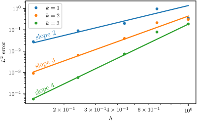
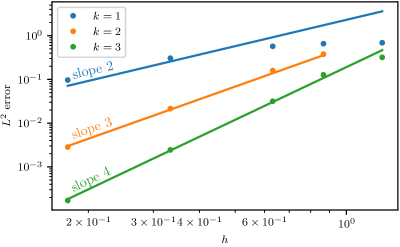
Figure 6.1. $L^{2}$ error for advection-diffusion problem for $d=2$ (top) and $d=3$ (bottom).

$h$	$\tau$	$L^{2}$ error	$H^{1}$ error	eoc($L^{2}$ error)	eoc($H^{1}$ error)
$1.00000$	$1.00000$	$3.51296\times 10^{-1}$	$3.30187$	—	—
$6.66667\times 10^{-1}$	$5.00000\times 10^{-1}$	$9.51874\times 10^{-1}$	$4.43031$	-2.458416	-0.725039
$4.37747\times 10^{-1}$	$2.50000\times 10^{-1}$	$1.99238\times 10^{-1}$	$2.33192$	3.717892	1.525683
$2.40008\times 10^{-1}$	$1.25000\times 10^{-1}$	$9.02047\times 10^{-2}$	$1.44891$	1.318576	0.791859
$1.34513\times 10^{-1}$	$6.25000\times 10^{-2}$	$2.78846\times 10^{-2}$	$7.80431\times 10^{-1}$	2.027605	1.068576

(a) Order 1, $d=2$

$h$	$\tau$	$L^{2}$ error	$H^{1}$ error	eoc($L^{2}$ error)	eoc($H^{1}$ error)
$1.00000$	$1.00000$	$3.05166\times 10^{-1}$	$3.29594$	—	—
$6.66667\times 10^{-1}$	$5.00000\times 10^{-1}$	$2.14128\times 10^{-1}$	$2.03484$	0.873768	1.189433
$4.37747\times 10^{-1}$	$2.50000\times 10^{-1}$	$3.93009\times 10^{-2}$	$8.61571\times 10^{-1}$	4.030255	2.043065
$2.40008\times 10^{-1}$	$1.25000\times 10^{-1}$	$6.51346\times 10^{-3}$	$2.89276\times 10^{-1}$	2.990807	1.816030
$1.34513\times 10^{-1}$	$6.25000\times 10^{-2}$	$9.24067\times 10^{-4}$	$8.43187\times 10^{-2}$	3.372712	2.129106

(b) Order 2, $d=2$

$h$	$\tau$	$L^{2}$ error	$H^{1}$ error	eoc($L^{2}$ error)	eoc($H^{1}$ error)
$1.00000$	$1.00000$	$1.87468\times 10^{-1}$	$2.57196$	—	—
$6.66667\times 10^{-1}$	$5.00000\times 10^{-1}$	$7.90234\times 10^{-2}$	$8.93941\times 10^{-1}$	2.130551	2.606354
$4.37747\times 10^{-1}$	$2.50000\times 10^{-1}$	$7.35252\times 10^{-3}$	$1.97059\times 10^{-1}$	5.645317	3.594764
$2.40008\times 10^{-1}$	$1.25000\times 10^{-1}$	$5.83518\times 10^{-4}$	$4.39236\times 10^{-2}$	4.216077	2.497725
$1.34513\times 10^{-1}$	$6.25000\times 10^{-2}$	$5.75918\times 10^{-5}$	$2.73132\times 10^{-2}$	3.999388	0.820506

(c) Order 3, $d=2$

$h$	$\tau$	$L^{2}$ error	$H^{1}$ error	eoc($L^{2}$ error)	eoc($H^{1}$ error)
$1.25000$	$1.00000$	$6.90651\times 10^{-1}$	$8.44875$	—	—
$8.66599\times 10^{-1}$	$5.00000\times 10^{-1}$	$6.57464\times 10^{-1}$	$7.69389$	0.134429	0.255490
$6.31590\times 10^{-1}$	$2.50000\times 10^{-1}$	$5.72385\times 10^{-1}$	$6.68398$	0.438071	0.444822
$3.33531\times 10^{-1}$	$1.25000\times 10^{-1}$	$3.05710\times 10^{-1}$	$4.43667$	0.982256	0.641827
$1.75870\times 10^{-1}$	$6.25000\times 10^{-2}$	$9.68233\times 10^{-2}$	$2.34095$	1.796513	0.998992

(d) Order 1, $d=3$

$h$	$\tau$	$L^{2}$ error	$H^{1}$ error	eoc($L^{2}$ error)	eoc($H^{1}$ error)
$8.66599\times 10^{-1}$	$5.00000\times 10^{-1}$	$3.78772\times 10^{-1}$	$5.39342$	—	—
$6.31590\times 10^{-1}$	$2.50000\times 10^{-1}$	$1.59518\times 10^{-1}$	$2.89154$	2.733729	1.970655
$3.33531\times 10^{-1}$	$1.25000\times 10^{-1}$	$2.14372\times 10^{-2}$	$9.12177\times 10^{-1}$	3.143326	1.806895
$1.75870\times 10^{-1}$	$6.25000\times 10^{-2}$	$2.84564\times 10^{-3}$	$2.57151\times 10^{-1}$	3.155269	1.978425

(e) Order 2, $d=3$

$h$	$\tau$	$L^{2}$ error	$H^{1}$ error	eoc($L^{2}$ error)	eoc($H^{1}$ error)
$1.25000$	$1.00000$	$3.19819\times 10^{-1}$	$4.78209$	—	—
$8.66599\times 10^{-1}$	$5.00000\times 10^{-1}$	$1.27429\times 10^{-1}$	$2.73209$	2.511984	1.528193
$6.31590\times 10^{-1}$	$2.50000\times 10^{-1}$	$3.16946\times 10^{-2}$	$9.05805\times 10^{-1}$	4.398523	3.489946
$3.33531\times 10^{-1}$	$1.25000\times 10^{-1}$	$2.44323\times 10^{-3}$	$1.41707\times 10^{-1}$	4.013792	2.905320
$1.75870\times 10^{-1}$	$6.25000\times 10^{-2}$	$1.70045\times 10^{-4}$	$2.10221\times 10^{-2}$	4.164150	2.981596

(f) Order 3, $d=3$

Table 6.1. Results for advection-diffusion problem for $d=2,3$.

Author contributions

Conceptualization, investigation, formal analysis, writing: All. Software: TR. Supervision: CME. Writing (first draft): PS.

Appendix A Proof of Regularity

In this section, we will show some results on the additional regularity of the smooth solution to 4.2.

Lemma A.1 (The Trace Map).

There exists a bounded and continuous linear operator $\widetilde{\tau}_{(\cdot)}:L^{2}_{V}\to L^{2}_{\mathcal{V}_{\Gamma}}$ such that $\widetilde{\tau}_{t}\varphi(t)=\tau_{t}\varphi(t)$ $\forall\varphi\in C_{V}$, where $\tau_{t}:V(t)\to\mathcal{V}_{\Gamma}(t)$ is the classical trace map.

Proof.

Let $\tau_{t}:V(t)\to\mathcal{V}_{\Gamma}(t)$ be the classical trace map. It is proven in [7] that the following identity: $\tau_{t}(\phi_{t}w_{0})=\phi_{t}(\tau_{0}w_{0})$ holds for all $t\in I$ and $w_{0}\in V(0)$. Moreover, there exists a $c$ independent of time such that:

$$\|\tau_{t}(\phi_{t}w_{0})\|_{\mathcal{H}_{\Gamma}(t)}\leq c\|\phi_{t}w_{0}\|_{\mathcal{V}_{\Gamma}(t)}.$$

Now, formally define $\widetilde{\tau}_{(\cdot)}$ as:

$$\widetilde{\tau}_{(\cdot)}v(\cdot)=\phi_{(\cdot)}\tau_{0}(\phi_{-(\cdot)}v(\cdot)).$$

Then via Lem. 2.2, $\phi_{-(\cdot)}v(\cdot)\in L^{2}(I;V(0))$ and since $\tau_{0}$ can also furthermore be uniquely identified as a linear map $\tau_{0}:L^{2}(I;V(0))\to L^{2}(I;\mathcal{V}_{\Gamma}(0))$, see [32, Thm. 1.2.4], finally the push-forward $\phi_{t}:L^{2}(I;\mathcal{V}_{\Gamma}(0))\to L^{2}_{\mathcal{V}_{\Gamma}}$ maps back into the evolving space. Note that this map, by compatibility and it’s time independent bound is also bounded. Finally, if $\varphi\in C_{V}$, then, at time $t\in I$:

$$\widetilde{\tau}_{t}\varphi(t)=\phi_{t}\tau_{0}(\phi_{-t}\varphi(t))=\tau_{t}\varphi(t).\quad\qed$$

This allows us to formally identify the following pairing:

$$\int_{0}^{T}\langle g,v\rangle_{\mathcal{V}_{\Gamma}(t)}:=\int_{0}^{T}\langle g,\widetilde{\tau}_{t}v\rangle_{\mathcal{V}_{\Gamma}(t)},\;(g,v)\in L^{2}_{\mathcal{V}^{*}_{\Gamma}}\times L^{2}_{V}.$$

Lemma A.2.

Under the assumptions of $A4$ Thm. 2.16, for each $g\in L^{2}_{\mathcal{V}_{\Gamma}}$, there exists a unique solution $u_{g}\in L^{2}_{Z_{1}}$ to:

$$\sum_{i=1}^{2}\int_{0}^{T}\int_{\Omega_{i}(t)}\mathcal{A}_{i}(t;x)\nabla u_{g}\cdot\nabla v=\int_{0}^{T}\int_{\Gamma(t)}gv\quad\text{for all}\quad v\in L^{2}_{V}.$$ (A.1)

Proof.

It follows from the regularity assumptions on the flow $\mathbf{\Phi}_{t}$ that the pair $(Z_{1}(t),\phi_{t}|_{Z_{1}(t)})|_{t\in I}$ is compatible. For $g\in L^{2}_{\mathcal{V}_{\Gamma}}$, we can take a subset $I^{\prime}\subset I$ of full measure such that $g(t)\in\mathcal{V}_{\Gamma}(t)$ and $\|g(t)\|_{\mathcal{V}_{\Gamma}(t)}<\infty$, for $t\in I^{\prime}$. Indeed via Lem. 2.2, we can take the set of Lebesgue points of $\widetilde{g}(\cdot)=\phi_{-(\cdot)}g(\cdot)$ to be $I^{\prime}$ and push the function forwards, $g(t)=\phi_{t}\widetilde{g}(t)\in\mathcal{V}_{\Gamma}(t)$ for all $t\in I^{\prime}$. Moreover, we see that, for $t\in I^{\prime}$, these remain Lebesgue Points of $\|g(\cdot)\|_{\mathcal{V}_{\Gamma}(\cdot)}$ in $L^{2}(I)$, indeed, via the reverse triangle inequality and compatibility:

$$\frac{1}{2\delta}\int_{t-\delta}^{t+\delta}|\|g\|_{\mathcal{V}_{\Gamma}(s)}-\|g\|_{\mathcal{V}_{\Gamma}(t)}|^{2}\,ds \leq\frac{c}{2\delta}\int_{t-\delta}^{t+\delta}|\|\widetilde{g}(s)\|_{\mathcal{V}_{\Gamma}(0)}-\|\widetilde{g}(t)\|_{\mathcal{V}_{\Gamma}(0)}|^{2}\,ds$$

$$\leq\frac{c}{2\delta}\int_{t-\delta}^{t+\delta}\|\widetilde{g}(s)-\widetilde{g}(t)\|_{\mathcal{V}_{\Gamma}(0)}^{2}\,ds$$

Fix $t\in I^{\prime}$, set $u^{t}_{g}\in V(t)$ to be the solution to:

$$\sum_{i=1}^{2}\int_{\Omega_{i}(t)}\mathcal{A}(t;x)\nabla u^{t}_{g}\cdot\nabla v=\int_{\Gamma(t)}gv\leavevmode\nobreak\ \leavevmode\nobreak\ \forall\leavevmode\nobreak\ v\in V(t).$$ (A.2)

We will drop the distinction between $I^{\prime}$ and $I$ and just say for almost all $t\in I$, then via the Hilbert triple structure outlined in Sec. 2.3, $g(t)\in\mathcal{V}_{\Gamma}(t)\subset\mathcal{H}_{\Gamma}(t)\subset\mathcal{V}^{*}_{\Gamma}(t)$. By [38, Thm. 1] we have that for almost all $t\in I$ there exists a unique solution $u^{t}_{g}(\cdot)\in Z_{1}(t)$ to A.2.

Set $u_{g}(t;\cdot):=u^{t}_{g}(\cdot)$, we show that this solution is in-fact in $L^{2}_{Z_{1}}$. We will proceed as follows:

1. First show that $u_{g}\in L^{2}_{V}$. By [5, Lem. 2.14], it suffices to show first that $t\to(u_{g},w)_{V(t)}$ is measurable for all $w\in L^{2}_{V}$ and then that $\|u_{g}\|_{L^{2}_{V}}<\infty$.

2. We then reuse this method, showing that $t\to(u_{g},w)_{Z_{1}(t)}$ is measurable for all $w\in L^{2}_{Z_{1}}$ and $\|u_{g}\|_{L^{2}_{Z_{1}}}<\infty$, and hence $u_{g}\in L^{2}_{Z_{1}}$.

3. Finally, we show that $u_{g}$ does indeed solve A.1.

To show the measurability, since the eigenvalues of $\mathcal{A}_{i}(t;x)$ are bounded from both below and above independent of time, we can induce the equivalent inner product $(u,v)_{\widetilde{V}(t)}:=(\mathcal{A}(t;x)\nabla u,\nabla v)_{H(t)}$. Showing measurability then follows as:

$$(u_{g},v)_{\widetilde{V}(t)}=\sum_{i=1}^{2}\int_{\Omega_{i}(t)}\mathcal{A}_{i}(t;x)\nabla u_{g}\cdot\nabla v=\int_{\Gamma(t)}gv=\int_{\Gamma(t)}\langle g,v\rangle_{\mathcal{V}_{\Gamma}(t)},$$

and since $(v,g)\in L^{2}_{V}\times L^{2}_{\mathcal{V}_{\Gamma}^{*}}$, by [5, Lem. 2.14], the map $t\mapsto\langle g,v\rangle_{\mathcal{V}_{\Gamma}(t)}$ is measurable and hence so is $(u_{g},v)_{\widetilde{V}(t)}$. For the uniform bound, testing the differential equation A.2 with $v=u_{g}$ and integrating in time, we have:

$$\|u_{g}\|^{2}_{L^{2}_{V}}\leq C(\gamma)\|g\|^{2}_{L^{2}_{\mathcal{V}_{\Gamma}^{*}}},$$

via Young’s and Poincaré’s inequalities, so $u_{g}\in L^{2}_{V}$. Before moving on, note that for any fixed $t\in I$, since $u_{g}(t;\cdot)\in Z_{1}(t)$, we can integrate by parts A.2, obtaining:

$$\int_{\Gamma(t)}\bigg{\llbracket}\mathcal{A}(t;x)\nabla u\cdot\nu_{\Gamma}\bigg{\rrbracket}v-\sum_{i=1}^{2}\int_{\Omega_{i}(t)}\nabla\cdot(\mathcal{A}_{i}(t;x)\nabla u_{g})v=\int_{\Gamma(t)}gv,$$ (A.3)

for $v\in C^{\infty}_{0}(\Omega)$. For $v\in C^{\infty}_{0}(\Omega_{1}(t))\times C^{\infty}_{0}(\Omega_{2}(t))$, we see that A.3 yields:

$$\sum_{i=1}^{2}\int_{\Omega_{i}(t)}\nabla\cdot(\mathcal{A}_{i}(t;x)\nabla u_{g})v=0.$$

Since the space $C^{\infty}_{0}(\Omega_{1}(t))\times C^{\infty}_{0}(\Omega_{2}(t))$ is dense in $H(t)$, we get that:

$$\nabla\cdot(\mathcal{A}_{i}(t;x)\nabla u_{g})=0\;\text{a.e}.$$ (A.4)

By the Poincaré’s inequality, we can endow $Z_{1}(t)$ with a more convenient equivalent inner product:

$$(v,w)_{Z_{1}(t)}=\sum_{i=1}^{2}\int_{\Omega_{i}(t)}\Delta v\cdot\Delta w+\nabla v\cdot\nabla w.$$

Since $\mathcal{A}(t;x)$ is assumed to be differentiable, we introduce the equivalent inner product on $Z_{1}(t)$:

$$(\eta,v)_{\widetilde{Z}_{1}(t)}:=\\ \sum_{i=1}^{2}\int_{\Omega_{i}(t)}\nabla\cdot(\mathcal{A}_{i}(t;x)\nabla\eta_{i})\nabla\cdot(\mathcal{A}_{i}(t;x)\nabla v_{i})+(\nabla\mathcal{A}_{i}(t;x))\cdot\nabla\eta_{i}(\nabla\mathcal{A}_{i}(t;x))\cdot\nabla v_{i}+\nabla\eta_{i}\cdot\nabla v_{i}.$$

We will first show the following statement, let $\nabla^{2}$ be the Hessian, then:

$$\int_{\Omega_{i}(t)}|\mathcal{A}_{i}\nabla^{2}\eta_{i}|^{2}\geq\gamma\int_{\Omega_{i}(t)}|\Delta\eta_{i}|^{2},$$

where $\gamma>0$ is the coercivity constant in Thm. 2.16. For fixed $t\in I$, since $\mathcal{A}_{i}(t;x)$ is non-singular and symmetric, there exists orthogonal matrices $\mathcal{P}_{i}(t;x)$, $\mathcal{P}_{i}^{T}(t;x)$ and diagonal matrix $\mathcal{D}_{i}(t;x)=[\lambda_{k}(t;x)\delta_{k,l}]_{k,l=1}^{n}$, the eigenvalues of $\mathcal{A}_{i}(t;x)$ (note that eigenvalues are continuous for a continuous matrix) such that $\mathcal{A}_{i}(t;x)=\mathcal{P}_{i}(t;x)\mathcal{D}_{i}(t;x)\mathcal{P}^{T}_{i}(t;x)$. Doing a change of coordinates, $x=\mathcal{P}_{i}y$ and letting $\tilde{\eta}_{i}(x)=\eta_{i}(\mathcal{P}_{i}(x))$, we see:

$$\mathcal{A}_{i}(t;x)\nabla^{2}(\eta_{i}(x))=\mathcal{D}_{i}(t;x)\Delta\tilde{\eta}_{i}(y)|_{y=\mathcal{P}_{i}^{T}x}.$$

Hence, since $\mathcal{P}$ is orthogonal:

$$\int_{\Omega_{i}(t)}|\mathcal{A}_{i}(t;x)\nabla^{2}(\eta_{i}(x))|^{2}\,dx =\int_{\mathcal{P}_{i}^{T}(\Omega_{i}(t))}|\mathcal{D}_{i}(t;\mathcal{P}_{i}(y))\Delta\tilde{\eta}_{i}(y)|^{2}\,dy,$$

$$\geq\min_{x\in\Omega_{i}(t)}\min_{k\in[1,n]}\lambda^{2}_{k}(t;\mathcal{P}_{i}^{T}(x))\int_{\mathcal{P}_{i}^{T}(\Omega_{i}(t))}|\Delta\tilde{\eta}_{i}(y)|^{2}\,dy,$$

$$\geq\gamma^{2}\int_{\mathcal{P}^{T}(\Omega_{i}(t))}|\Delta\tilde{\eta}_{i}(y)|^{2}\,dy=\gamma^{2}\int_{\Omega_{i}(t)}|\Delta\eta_{i}(x)|^{2}\,dx.$$

To show the equivalence of inner products $(\cdot,\cdot)_{\widetilde{Z}_{1}(t)}$ and $(\cdot,\cdot)_{Z_{1}(t)}$, note:

$$\|\eta\|^{2}_{\widetilde{Z}_{1}(t)} =\sum_{i=1}^{2}\int_{\Omega_{i}(t)}|\nabla\cdot(\mathcal{A}_{i}(t;x)\nabla\eta_{i})|^{2}+|(\nabla\mathcal{A}_{i}(t;x))\cdot\nabla\eta_{i}|^{2}+|\nabla\eta_{i}|^{2}$$

$$=\sum_{i=1}^{2}\int_{\Omega_{i}(t)}|\mathcal{A}_{i}(t;x)\nabla^{2}\eta_{i}|^{2}+2\mathcal{A}_{i}(t;x)\nabla^{2}\eta_{i}(\nabla\mathcal{A}_{i}(t;x))\cdot\nabla\eta_{i}+2|(\nabla\mathcal{A}_{i}(t;x))\cdot\nabla\eta_{i}|^{2}+|\nabla\eta_{i}|^{2}$$

$$\geq\sum_{i=1}^{2}\int_{\Omega_{i}(t)}\tfrac{1}{2}|\mathcal{A}_{i}(t;x)\nabla^{2}\eta_{i}|^{2}+|\nabla\eta_{i}|^{2}\geq\min\left\{\tfrac{1}{2}\gamma^{2},1\right\}\|\eta\|^{2}_{Z_{1}(t)}$$

and:

$$\|\eta\|^{2}_{\widetilde{Z}_{1}(t)}\leq c\left[|\mathcal{A}_{i}|_{C^{1}(\Omega_{i}(t))}\right](\|\nabla^{2}\eta_{i}\|^{2}_{H(t)}+\|\nabla\eta_{i}\|^{2}_{H(t)})\leq c\|\eta\|^{2}_{Z_{1}(t)}.$$

Hence, $(\cdot,\cdot)_{\tilde{Z}_{1}(t)}$ and $(\cdot,\cdot)_{Z(t)}$ are equivalent. Substituting $\eta=u_{g}$ in the new inner product, using A.4, we arrive at:

$$(u_{g},v)_{\widetilde{Z}_{1}(t)}=\sum_{i=1}^{2}\int_{\Omega_{i}(t)}(\nabla\mathcal{A}_{i}(t;x))\cdot\nabla u_{i}(\nabla\mathcal{A}_{i}(t;x))\cdot\nabla v_{i}+\nabla u_{i}\cdot\nabla v_{i}.$$

Since we already know that $u_{g}\in L^{2}_{V}$, both $((\nabla\mathcal{A}(t;x))\cdot\nabla u,(\nabla\mathcal{A}(t;x))\cdot\nabla v)_{H(t)}$ and $(\nabla u,\nabla v)_{H(t)}$ are measurable and hence the map $t\to(u_{g},v)_{\widetilde{Z}_{1}(t)}$ is measurable for all $v\in Z_{1}(t)$. For the bound, [38, Thm. 1] gives us a constant $C_{t}$ (that depends on time) such that:

$$\|u_{g}\|_{Z_{1}(t)}\leq C_{t}\|g\|_{\mathcal{V}_{\Gamma}(t)}.$$

Using a similar method as Lem. 2.12 and changing the variables, it follows that there exists $C_{T}>C_{t}$, $C_{T}<\infty$. Hence:

$$\int_{0}^{T}\|u_{g}\|_{Z_{1}(t)}^{2}\leq C_{T}^{2}\int_{0}^{T}\|g\|_{\mathcal{V}_{\Gamma}(t)}^{2}<\infty.$$

Hence $u_{g}\in L^{2}_{Z_{1}}$.

Finally, we have a solution to $u_{g}\in L^{2}_{Z_{1}}$ solving A.2 a.e in time. Since a function $v\in L^{2}_{V}$ satisfies $v(t)\in V(t)$ a.e in time, testing with such a $v(t)$ and integrating both sides of A.2 yields the desired solution. Uniqueness follows via coercivity. ∎

Lemma A.3.

Under the assumption $A4$ from Thm. 2.16, the solution of A.1 posses a weak material derivative $\partial_{t}^{\bullet}u_{g}\in L^{2}_{V}$ and satisfies the estimate:

$$\|u_{g}\|^{2}_{W(Z_{1},V)}\leq c\|g\|^{2}_{W(\mathcal{V}_{\Gamma},\mathcal{V}_{\Gamma}^{*})}$$

Proof.

We use the same method as in the proof of Lem. 5.4. Let:

$$k(t;v,w):=\sum_{i=1}^{2}\int_{\Omega_{i}(t)}\mathcal{A}_{i}(t;x)\nabla v\cdot\nabla w$$

then we see, going back to A.2, we see that $u_{g}$ solves:

$$k(t;u_{g},w)=(g,w)_{\mathcal{H}_{\Gamma}(t)},$$

a.e for all $w\in L^{2}_{V}$ (as before, we can take a subset of $I$ of full measure such that $w(t)\in V(t)$, moreover, via the classical trace theorem, we can identify $w(t)\in\mathcal{H}_{\Gamma}(t)$ by $(g,w)_{\mathcal{H}_{\Gamma}(t)}=(g,\tau_{t}w)_{\mathcal{H}_{\Gamma}(t)}$). The derivative of $k(t;\cdot,\cdot)$, $\dot{k}(t;\cdot,\cdot)$, can be explicitly calculated to be:

$$\frac{d}{dt}k(t;w,v) =\dot{k}(t;w,v)+k(t;\partial_{t}^{\bullet}w,v)+k(t;w,\partial_{t}^{\bullet}v),\;\forall v,w\in W(V,V),$$ (A.5)

where

$$\dot{k}(t;w,v)=\sum_{i=1}^{2}\int_{\Omega_{i}(t)}\mathcal{D}^{\mathcal{A}}_{i}(\mathbf{w},\mathcal{A}_{i},w_{i},v_{i}),$$

and $\mathcal{D}^{\mathcal{A}}_{i}$ was defined in 2.12. We set $\tilde{u}_{g}$ to be the solution to:

$$\int_{0}^{T}k(t;\tilde{u}_{g},\eta)\,dt=\int_{0}^{T}\lambda_{\Gamma}(t;g,\eta)-\dot{k}(t;u_{g},\eta)+\langle\partial_{t}^{\bullet}g,\eta\rangle_{\mathcal{V}_{\Gamma}(t)}\,dt\quad\forall\eta\in L^{2}_{V}.$$ (A.6)

The material derivative taken on the function $\partial_{t}^{\bullet}g$ is the one with the triple $L^{2}_{\mathcal{V}_{\Gamma}}\subset L^{2}_{\mathcal{H}_{\Gamma}}\subset L^{2}_{V^{*}_{\Gamma}}$ and the bilinear form $\lambda_{\Gamma}$ is the corresponding form from Def. 2.3 satisfing the equation:

$$\frac{d}{dt}(v,w)_{\mathcal{H}_{\Gamma}(t)}=\langle\partial_{t}^{\bullet}v,w\rangle_{\mathcal{V}_{\Gamma}(t)}+\langle\partial_{t}^{\bullet}w,v\rangle_{\mathcal{V}_{\Gamma}(t)}+\lambda_{\Gamma}(t;v,w).$$

See [6, Sec. 5.4] for an explicit form of $\lambda_{\Gamma}(t;\cdot,\cdot)$. Using the same method as the proof of Lem. A.2, we have that if $\partial^{\bullet}_{t}g\in L^{2}_{\mathcal{V}_{\Gamma}^{*}}$, there exists a unique $\widetilde{u}_{g}\in L^{2}_{V}$ solving equation A.6.

Let $u_{g}$ be the solution of A.2. Via isomorphism, $\phi_{-(\cdot)}\tilde{u}_{g}(\cdot),\phi_{-(\cdot)}u_{g}(\cdot)\in L^{2}(I;V(0))$, we pick a Lebesgue point $s_{*}\in I$ of $\phi_{-(\cdot)}u_{g}(\cdot)$ and set

$$w:=\phi_{t}\int_{s_{*}}^{t}\phi_{-\tau}\widetilde{u}_{g}(\tau)\,d\tau+\phi_{t}\phi_{-s_{*}}u_{g}(s_{*})=\phi_{t}\int_{s_{*}}^{t}\phi_{-\tau}\widetilde{u}_{g}(\tau)\,d\tau+z_{s_{*}}.$$

Thus $w\in W(V,V)$ and $\partial_{t}^{\bullet}w=\tilde{u}_{g}$. We aim to show that $w=u_{g}$. To do so, note that by definition of $\dot{k}(t;\cdot,\cdot)$ A.5, testing with $\eta\in W(V,V)$ with $\eta(0)=\eta(T)=0$:

$$\int_{0}^{T}k(t;\partial_{t}^{\bullet}w,\eta)\,dt=\int_{0}^{T}-\dot{k}(t;w,\eta)-k(t;w,\partial_{t}^{\bullet}\eta)\,dt.$$ (A.7)

we see from comparing A.7 and A.6:

$$-\int_{0}^{T}k(t;w,\partial_{t}^{\bullet}\eta)\,dt=\int_{0}^{T}\dot{k}(t;w-u_{g},\eta)-(\partial_{t}^{\bullet}\eta,g)_{\mathcal{H}_{\Gamma}(t)}\,dt,\quad\forall\eta\in W(V,V),\;\eta(0)=\eta(T)=0.$$ (A.8)

Comparing A.8 with A.2, we infer:

$$\int_{0}^{T}k(t;u_{g}-w,\partial_{t}^{\bullet}\eta)\,dt=\int_{0}^{T}\dot{k}(t;w-u_{g},\eta)\,dt.$$

Letting $\eta(t)=\psi(t)v(t)$ where $\psi(t)\in\mathcal{D}(I)$ and $v(t)\in W(V,V)$, we see:

$$\int_{0}^{T}\psi(t)k(t;u_{g}-w,\partial_{t}^{\bullet}v)+\psi^{\prime}(t)k(t;u_{g}-w,v)\,dt=\int_{0}^{T}\psi(t)\dot{k}(t;w-u_{g},v)\,dt.$$

Since this holds for arbitrary $\psi\in\mathcal{D}(I)$, then, by use of [34, Lem. 1.2.1], there exists some $c\in\mathbb{R}$ such that:

$$k(t;u_{g}-w,v)=\int_{s_{*}}^{t}\dot{k}(\tau;w-u_{g},v)+k(\tau;w-u_{g},\partial_{t}^{\bullet}v)\,d\tau+c,$$ (A.9)

a.e in time. Note that the right hand side of A.9 is absolutely continuous in time and hence is the unique continuous representative of $k(t;u_{g}-w,v)$ (since $k(\cdot;u_{g}-w,v)$ is in $L^{1}(I)$ as a function of time). It also follows from the fact that $k(t;\eta,v)$ is continuous for $\eta,v\in C^{0}_{V}$ that $s_{*}$ is also a Lebesgue point of $k(t;u_{g}-w,v)$ (by use of a standard density argument). Since the continuous representative equals its $L^{p}$ counterpart on Lebesgue point (as Lebesgue points are also points of approximate continuity, see [24, Sec. 1.7]), evaluating both sides of A.9 at $t=s_{*}$, using the definition of $w$, yields $c=0$. Finally we can test with $\eta(s)=\phi_{s}\phi_{-t}(u_{g}-w)$ and by use of the same argument as Lem. 5.4 we see that $u_{g}=w$ and hence $u_{g}\in W(Z_{1},V)$. ∎

From the previous two lemmas, we can show a time regularity result for 4.2.

Lemma A.4.

Under the assumptions $A1$ to $A4$ in Thm. 2.16, the solution $u$ to problem 2.8 posses the additional regularity $u\in W(V,H)$.

Proof.

Let $z=u-u_{g}$, where $u$ is the weak solution from the problem in 2.8, then:

$$\int_{0}^{T}\langle\partial_{t}^{\bullet}z,v\rangle_{V(t)}+a(t;z,v)+\lambda(t;z,v)=\int_{0}^{T}\widetilde{l}(t;v),$$

where:

$$\widetilde{l}(t;v)=(f,v)_{H(t)}-(\partial^{\bullet}_{t}u_{g},v)_{H(t)}-\lambda(t;u_{g},v)-([\mathcal{B}-\mathbf{w}]\cdot\nabla u_{g}-[\mathcal{C}-\nabla\cdot\mathbf{w}]u_{g},v)_{H(t)}.$$

By the regularity of $u_{g}$, this is a functional in $L^{2}_{H}$, by [5, Thm. 3.13], $z\in W(V,H)$ and hence so is $u\in W(V,H)$. ∎

References

- [1]
- Abels et al. [2017] Helmut Abels, Harald Garcke, Kei Fong Lam, and Josef Weber. 2017. Two-Phase Flow with Surfactants: Diffuse Interface Models and Their Analysis. In Transport Processes at Fluidic Interfaces. Springer International Publishing, 255–270. https://doi.org/10.1007/978-3-319-56602-3_10
- Adjerid et al. [2015] Slimane Adjerid, Nabil Chaabane, and Tao Lin. 2015. An immersed discontinuous finite element method for Stokes interface problems. Comput. Methods Appl. Mech. Engrg. 293 (2015), 170–190. https://doi.org/10.1016/j.cma.2015.04.006
- Alphonse et al. [2023] Amal Alphonse, Diogo Caetano, Ana Djurdjevac, and Charles M. Elliott. 2023. Function spaces, time derivatives and compactness for evolving families of Banach spaces with applications to PDEs. Journal of Differential Equations 353 (2023), 268–338. https://doi.org/10.1016/j.jde.2022.12.032
- Alphonse et al. [2015a] Amal Alphonse, Charles Elliott, and Björn Stinner. 2015a. An abstract framework for parabolic PDEs on evolving spaces. Portugal. Math. 72, 1 (2015), 1–46. https://doi.org/10.4171/pm/1955
- Alphonse et al. [2015b] Amal Alphonse, Charles Elliott, and Björn Stinner. 2015b. On some linear parabolic PDEs on moving hypersurfaces. Interface. Free Bound. 17, 2 (2015), 157–187. https://doi.org/10.4171/ifb/338
- Alphonse et al. [2015c] Amal Alphonse, Charles M. Elliott, and Björn Stinner. 2015c. On some linear parabolic PDEs on moving hypersurfaces. Interfaces Free Bound. 17, 2 (2015), 157–187. https://doi.org/10.4171/IFB/338
- Balay et al. [2019] Satish Balay, Shrirang Abhyankar, Mark F. Adams, Jed Brown, Peter Brune, Kris Buschelman, Lisandro Dalcin, Victor Eijkhout, William D. Gropp, Dmitry Karpeyev, Dinesh Kaushik, Matthew G. Knepley, Dave A. May, Lois Curfman McInnes, Richard Tran Mills, Todd Munson, Karl Rupp, Patrick Sanan, Barry F. Smith, Stefano Zampini, Hong Zhang, and Hong Zhang. 2019. PETSc Users Manual. Technical Report ANL-95/11 - Revision 3.11. Argonne National Laboratory.
- Balay et al. [1997] Satish Balay, William D. Gropp, Lois Curfman McInnes, and Barry F. Smith. 1997. Efficient Management of Parallelism in Object Oriented Numerical Software Libraries. In Modern Software Tools in Scientific Computing, E. Arge, A. M. Bruaset, and H. P. Langtangen (Eds.). Birkhäuser Press, 163–202.
- Barrett et al. [2008] John W. Barrett, Harald Garcke, and Robert Nürnberg. 2008. On the parametric finite element approximation of evolving hypersurfaces in . J. Comput. Phys. 227, 9 (2008), 4281–4307. https://doi.org/10.1016/j.jcp.2007.11.023
- Barrett et al. [2014] John W. Barrett, Harald Garcke, and Robert Nürnberg. 2014. Stable phase field approximations of anisotropic solidification. IMA J. Numer. Anal. 34, 4 (2014), 1289–1327. https://doi.org/10.1093/imanum/drt044
- Barrett et al. [2015] John W. Barrett, Harald Garcke, and Robert Nürnberg. 2015. On the stable numerical approximation of two-phase flow with insoluble surfactant. ESAIM Math. Model. Numer. Anal. 49, 2 (2015), 421–458. https://doi.org/10.4208/cicp.190313.010813a
- Braess [2007] Dietrich Braess. 2007. Finite elements (third ed.). Cambridge University Press, Cambridge. xviii+365 pages. https://doi.org/10.1017/CBO9780511618635 Theory, fast solvers, and applications in elasticity theory, Translated from the German by Larry L. Schumaker.
- Brenner and Scott [2008] Susanne C. Brenner and L. Ridgway Scott. 2008. The mathematical theory of finite element methods (third ed.). Texts in Applied Mathematics, Vol. 15. Springer, New York. xviii+397 pages. https://doi.org/10.1007/978-0-387-75934-0
- Ciarlet and Raviart [1972] P. G. Ciarlet and P.-A. Raviart. 1972. The combined effect of curved boundaries and numerical integration in isoparametric finite element methods. In The mathematical foundations of the finite element method with applications to partial differential equations (Proc. Sympos., Univ. Maryland, Baltimore, Md., 1972), A. K. Aziz (Ed.). Academic Press, New York, 409–474.
- Dalcin et al. [2011] Lisandro D. Dalcin, Rodrigo R. Paz, Pablo A. Kler, and Alejandro Cosimo. 2011. Parallel distributed computing using Python. Adv. Water Resour. 34, 9 (Sept. 2011), 1124–1139. https://doi.org/10.1016/j.advwatres.2011.04.013 New Computational Methods and Software Tools.
- Douglas and Dupont [1973] Jim Douglas and Todd Dupont. 1973. Galerkin methods for parabolic equations with nonlinear boundary conditions. Numer. Math. 20, 3 (June 1973), 213–237. https://doi.org/10.1007/bf01436565
- Dziuk and Elliott [2012] Gerhard Dziuk and Charles M. Elliott. 2012. A fully discrete evolving surface finite element method. SIAM J. Numer. Anal. 50, 5 (2012), 2677–2694. https://doi.org/10.1137/110828642
- Edelmann [2021] Dominik Edelmann. 2021. Finite element analysis for a diffusion equation on a harmonically evolving domain. IMA J. Numer. Anal. 42, 2 (May 2021), 1866–1901. https://doi.org/10.1093/imanum/drab026 arXiv:2009.11105 [math.NA]
- Elliott and Fritz [2016] C. M. Elliott and H. Fritz. 2016. On algorithms with good mesh properties for problems with moving boundaries based on the Harmonic Map Heat Flow and the DeTurck trick. SMAI Journal of Computational Mathematics 2 (2016), 141–176.
- Elliott and Fritz [2017] Charles M. Elliott and Hans Fritz. 2017. On approximations of the curve shortening flow and of the mean curvature flow based on the DeTurck trick. IMA J. Numer. Anal. 37, 2 (2017), 543–603. https://doi.org/10.1093/imanum/drw020
- Elliott and Ranner [2013] C. M. Elliott and T. Ranner. 2013. Finite element analysis for a coupled bulk–surface partial differential equation. IMA J. Numer. Anal. doi: 10.1093/imanum/drs022 (2013).
- Elliott and Ranner [2021] C M Elliott and T Ranner. 2021. A unified theory for continuous-in-time evolving finite element space approximations to partial differential equations in evolving domains. IMA J. Numer. Anal. 41, 3 (July 2021), 1696–1845. https://doi.org/10.1093/imanum/draa062
- Evans and Gariepy [1992] Lawrence C. Evans and Ronald F. Gariepy. 1992. Measure theory and fine properties of functions. CRC Press, Boca Raton, FL. viii+268 pages.
- Foote [1984] Robert L. Foote. 1984. Regularity of the distance function. Proc. Amer. Math. Soc. 92, 1 (1984), 153–155. https://doi.org/10.2307/2045171
- Geuzaine and Remacle [2009] Christophe Geuzaine and Jean-François Remacle. 2009. Gmsh: A 3-D finite element mesh generator with built-in pre- and post-processing facilities. Int. J. Numer. Meth. Eng. 79, 11 (May 2009), 1309–1331. https://doi.org/10.1002/nme.2579
- Gilbarg and Trudinger [2001] David Gilbarg and Neil S. Trudinger. 2001. Elliptic partial differential equations of second order. Springer-Verlag, Berlin. xiv+517 pages. Reprint of the 1998 edition.
- Gross and Reusken [2011] Sven Gross and Arnold Reusken. 2011. Numerical Methods for Two-phase Incompressible Flows. Springer Series In Computational Mathematics, Vol. 47. Springer Berlin Heidelberg. https://doi.org/10.1007/978-3-642-19686-7
- Gurtin [1988] Morton E. Gurtin. 1988. Toward a nonequilibrium thermodynamics of two-phase materials. Arch. Ration. Mech. An. 100, 3 (Sept. 1988), 275–312. https://doi.org/10.1007/bf00251518
- Häkkinen et al. [2019] Teemu J. Häkkinen, S. Susanna Sova, Ian J. Corfe, Leo Tjäderhane, Antti Hannukainen, and Jukka Jernvall. 2019. Modeling enamel matrix secretion in mammalian teeth. PLOS Computational Biology 15, 5 (05 2019), 1–12. https://doi.org/10.1371/journal.pcbi.1007058
- Hartman [2002] Philip Hartman. 2002. Ordinary differential equations. Classics in Applied Mathematics, Vol. 38. Society for Industrial and Applied Mathematics (SIAM), Philadelphia, PA. xx+612 pages. https://doi.org/10.1137/1.9780898719222 Corrected reprint of the second (1982) edition [Birkhäuser, Boston, MA; MR0658490 (83e:34002)], With a foreword by Peter Bates.
- Hytönen et al. [2016] Tuomas Hytönen, Jan van Neerven, Mark Veraar, and Lutz Weis. 2016. Analysis in Banach spaces. Vol. I. Martingales and Littlewood-Paley theory. Ergebnisse der Mathematik und ihrer Grenzgebiete. 3. Folge. A Series of Modern Surveys in Mathematics, Vol. 63. Springer, Cham. xvi+614 pages.
- Jean Donea and Rodrigez-Ferran [2004] J.-Ph. Ponthot Jean Donea, Antonio Huerta and A. Rodrigez-Ferran. 2004. Arbitrary Lagrangian-Eulerian Methods. In Encyclopedia of Computational Mechanics, R. de Borst E. Sterin and T.J.R. Hughes (Eds.). John Wiley & Sons, Inc., Chapter 14, 413–437.
- Jost and Li-Jost [1998] Jürgen Jost and Xianqing Li-Jost. 1998. Calculus of variations. Cambridge Studies in Advanced Mathematics, Vol. 64. Cambridge University Press, Cambridge. xvi+323 pages.
- Kimura [2008] Masato Kimura. 2008. Geometry of hypersurfaces and moving hypersurfaces in for the study of moving boundary problems. In Topics in mathematical modeling. Jind ich Nec̆as Cent. Math. Model. Lect. Notes, Vol. 4. Matfyzpress, Prague, 39–93.
- Kovács and Power Guerra [2016] Balázs Kovács and Christian Andreas Power Guerra. 2016. Error analysis for full discretizations of quasilinear parabolic problems on evolving surfaces. Numer. Meth. Part. D. E. 32, 4 (Feb. 2016), 1200–1231. https://doi.org/10.1002/num.22047
- Li et al. [2022] Buyang Li, Yinhua Xia, and Zongze Yang. 2022. Optimal convergence of arbitrary Lagrangian–Eulerian iso-parametric finite element methods for parabolic equations in an evolving domain. IMA J. Numer. Anal. 43, 1 (Jan. 2022), 501–534. https://doi.org/10.1093/imanum/drab099
- Li et al. [2013] H. Li, V. Nistor, and Y. Qiao. 2013. Uniform Shift Estimates for Transmission Problems and Optimal Rates of Convergence for the Parametric Finite Element Method. Lect. Notes. Comput. Sc. (2013), 12–23. https://doi.org/10.1007/978-3-642-41515-9_2
- MacDonald et al. [2016] G. MacDonald, J. A. Mackenzie, M. Nolan, and R. H. Insall. 2016. A computational method for the coupled solution of reaction-diffusion equations on evolving domains and manifolds: application to a model of cell migration and chemotaxis. J. Comput. Phys. 309 (2016), 207–226. https://doi.org/10.1016/j.jcp.2015.12.038
- Mikhailov [2011] Sergey E. Mikhailov. 2011. Traces, extensions and co-normal derivatives for elliptic systems on Lipschitz domains. J. Math. Anal. Appl. 378, 1 (2011), 324–342. https://doi.org/10.1016/j.jmaa.2010.12.027
- Mu and Zhang [2019] Lin Mu and Xu Zhang. 2019. An immersed weak Galerkin method for elliptic interface problems. J. Comput. Appl. Math. 362 (Dec. 2019), 471–483. https://doi.org/10.1016/j.cam.2018.08.023
- Nečas [1967] Jindřich Nečas. 1967. Les méthodes directes en théorie des équations elliptiques. Masson et Cie, Éditeurs, Paris; Academia, Éditeurs, Prague. 351 pages.
- Prüss and Simonett [2016] Jan Prüss and Gieri Simonett. 2016. Moving interfaces and quasilinear parabolic evolution equations. Monographs in Mathematics, Vol. 105. Birkhäuser/Springer, [Cham]. xix+609 pages. https://doi.org/10.1007/978-3-319-27698-4
- Ranner [2023] Thomas Ranner. 2023. firedrake moving interfaces. Zenodo. https://doi.org/10.5281/zenodo.8068963
- Rathgeber et al. [2017] Florian Rathgeber, David A. Ham, Lawrence Mitchell, Michael Lange, Fabio Luporini, Andrew T. T. Mcrae, Gheorghe-Teodor Bercea, Graham R. Markall, and Paul H. J. Kelly. 2017. Firedrake. ACM Trans. Math. Software 43, 3 (Jan. 2017), 1–27. https://doi.org/10.1145/2998441 arXiv:1501.01809
- Renardy and Rogers [2004] Michael Renardy and Robert C. Rogers. 2004. An introduction to partial differential equations (second ed.). Texts in Applied Mathematics, Vol. 13. Springer-Verlag, New York. xiv+434 pages.
- Roubicek [2005] T. Roubicek. 2005. Nonlinear Partial Differential Equations with Applications. International seies of numerical mathematics, Vol. 153. Birkhäuser-Verlag, Basel Boston Berlin. https://doi.org/10.1007/3-7643-7397-0
- Ryder et al. [2019] Lauren S. Ryder, Yasin F. Dagdas, Michael J. Kershaw, Chandrasekhar Venkataraman, Anotida Madzvamuse, Xia Yan, Neftaly Cruz-Mireles, Darren M. Soanes, Miriam Oses-Ruiz, Vanessa Styles, Jan Sklenar, Frank L. H. Menke, and Nicholas J. Talbot. 2019. A sensor kinase controls turgor-driven plant infection by the rice blast fungus. Nature 574, 7778 (Oct. 2019), 423–427. https://doi.org/10.1038/s41586-019-1637-x
- San Martín et al. [2009] Jorge San Martín, Loredana Smaranda, and Takéo Takahashi. 2009. Convergence of a finite element/ALE method for the Stokes equations in a domain depending on time. J. Comput. Appl. Math. 230, 2 (Aug. 2009), 521–545. https://doi.org/10.1016/j.cam.2008.12.021
- Schramm et al. [2003] Laurier L. Schramm, Elaine N. Stasiuk, and D. Gerrard Marangoni. 2003. 2 Surfactants and their applications. Annu. Rep. Prog. Chem., Sect. C: Phys. Chem. 99 (2003), 3–48. https://doi.org/10.1039/b208499f
- Werner et al. [2022] Philipp Werner, Martin Burger, Florian Frank, and Harald Garcke. 2022. A Diffuse Interface Model for Cell Blebbing Including Membrane-Cortex Coupling with Linker Dynamics. SIAM J. Appl. Math. 82, 3 (June 2022), 1091–1112. https://doi.org/10.1137/21m1433642
- Yang and Zhang [2016] Qing Yang and Xu Zhang. 2016. Discontinuous Galerkin immersed finite element methods for parabolic interface problems. J. Comput. Appl. Math. 299 (June 2016), 127–139. https://doi.org/10.1016/j.cam.2015.11.020 Recent Advances in Numerical Methods for Systems of Partial Differential Equations.