Automated Calculation of Beam Functions at NNLO

Abstract

We present an automated framework for the calculation of beam functions that describe collinear initial-state radiation at hadron colliders at next-to-next-to leading order (NNLO) in perturbation theory. By exploiting the infrared behaviour of the collinear matrix elements, we factorise the phase-space singularities with suitable observable-independent parametrisations. Our numerical approach applies to a large class of collider observables, and as a check of its validity, we compute the quark beam functions for transverse-momentum resummation and N-jettiness, which are known analytically at this order, finding excellent agreement.

1 Introduction

Beam functions constitute a key ingredient in factorisation theorems at hadron colliders. For the measurement of a global observable $\omega$ that is sensitive to soft and collinear QCD radiation, the differential cross section typically takes the following schematic form,

$$\frac{{\rm d}\sigma}{{\rm d}\omega}=H(Q)\cdot\prod_{i}B_{i/h}(\omega)\otimes\prod_{j}J_{j}(\omega)\otimes S(\omega)\,.$$ (1)

The hard function $H(Q)$ describes the virtual corrections to the Born process, and it depends only on the hard scale $Q$ of the process, while it is independent of the specific measurement $\omega$. On the other hand, the beam functions $B_{i/h}(\omega)$, the jet functions $J_{j}(\omega)$ and the soft function $S(\omega)$ describe initial-state collinear, final-state collinear and soft emissions, respectively, and they are observable-dependent. One thus needs to compute these functions on a case-by-case basis for each observable, which for the beam functions has been achieved either analytically [1, 2, 3, 4, 5, 6, 7, 8, 9, 10, 11] or semi-analytically [12, 13] in some cases relevant e.g. for transverse-momentum or jet-veto resummation. An automated approach for the calculation of beam functions at next-to-next-to-leading order (NNLO) in perturbation theory has been initiated only recently [14, 15], and in this article we report on the status of these developments.

An automated framework for the calculation of soft functions at NNLO is already available through the public package SoftSERVE [16, 17, 18]. This has been achieved by introducing suitable phase-space parametrisations to factorise the divergences of the soft matrix elements at the second order of the strong coupling. The singularity structure of the collinear matrix elements is, on the other hand, significantly more complicated. The beam functions are, moreover, defined as proton matrix elements of collinear field operators, and they need to be matched onto the standard parton distribution functions to extract the relevant perturbative information. By employing suitable phase-space parametrisations, sector-decomposition techniques and non-linear transformations, we recently set up a similar automated framework for the calculation of the beam-function matching kernels [14]. As a first application of our approach, we computed the quark beam function for jet-veto resummation [15], and in this work we present our results for transverse-momentum resummation and the event-shape variable N-jettiness. While these beam functions are known analytically at the considered NNLO for quite some time [2, 6], they provide important reference observables for our setup. In particular, they allow us to test the numerical accuracy of our predictions for different classes of observables, which are known as SCET-1 and SCET-2 beam functions.

2 Quark beam functions

We are concerned with quark beam functions that are defined via

$$\frac{1}{2}\left[\frac{{\not{n}}}{2}\right]_{\beta\alpha}{\cal B}_{q/h}(x,\tau,\mu)= \sum_{X}\,\delta\Big{(}(1-x)P^{-}-\sum_{i}k_{i}^{-}\Big{)}\,{\cal M}(\tau;\{k_{i}\})\bra{h(P)}\bar{\chi}_{\alpha}\ket{X}\bra{X}\chi_{\beta}\ket{h(P)},$$ (2)

where $\chi=W^{\dagger}_{\bar{n}}\frac{{\not{n}}{\not{\bar{n}}}}{4}\psi$ is the collinear quark field, and we used light-cone coordinates with $k_{i}^{-}=\bar{n}\cdot k_{i}$, $k_{i}^{+}=n\cdot k_{i}$ and a transverse component $k_{i}^{\perp,\mu}$ that satisfies $n\cdot k_{i}^{\perp}=\bar{n}\cdot k_{i}^{\perp}=0$, along with $n^{2}=\bar{n}^{2}=0$ and $n\cdot\bar{n}=2$. The sum over $X$ represents the phase space of the collinear emissions with momenta $\{k_{i}\}$, while the external state $\ket{h(P)}$ refers to a hadronic state with momentum $P^{\mu}=P^{-}n^{\mu}/2$. The function ${\cal M}(\tau;\{k_{i}\})$ furthermore specifies the observable, and in order to avoid distribution-valued expressions, we assume that it is given in Laplace space, with $\tau$ being the corresponding Laplace variable (see also [16, 17, 18]).

Unlike soft and jet functions, beam functions are intrinsically non-perturbative objects, but as long as the relevant scale of the collinear emissions is perturbative, i.e. $\tau\ll 1/\Lambda_{\rm QCD}$, they can be matched onto the usual parton distribution functions (pdf). The matching relation is most conveniently expressed in Mellin space, ${\cal\widehat{B}}_{q/h}(N,\tau,\mu)=\int_{0}^{1}dx\;x^{N-1}\;{\cal B}_{q/h}(x,\tau,\mu)$, where it becomes

$$\mathcal{\widehat{B}}_{q/h}(N,\tau,\mu) =\sum_{k}\,{\cal\widehat{I}}_{q\leftarrow k}(N,\tau,\mu)\leavevmode\nobreak\ \widehat{f}_{k/h}(N,\mu)\,,$$ (3)

and the sum runs over all partonic channels. The development of an automated framework to compute the matching kernels ${\cal\widehat{I}}_{q\leftarrow k}(N,\tau,\mu)$ to NNLO accuracy is the goal of the current project. The matching kernels can, in fact, be extracted from partonic rather than hadronic beam functions, i.e. the external states $\ket{h(P)}$ in (2) can be interpreted as partonic states for this purpose. If the matching is performed on-shell in dimensional regularisation, the partonic pdf evaluate to $\widehat{f}_{k/j}(N,\mu)=\delta_{kj}$ to all orders in perturbation theory, and the extraction of the matching kernels boils down to the calculation of the bare partonic beam functions.

Depending on the observable, dimensional regularisation may not be sufficient to resolve all phase-space singularities that appear in the beam-function calculation. It is well-known that one needs an additional prescription to regularise rapidity divergences for transverse-momentum dependent SCET-2 observables. In our approach, we regularise these divergences with a symmetric version of the phase-space regulator proposed in [19]. We thus introduce the following phase-space factor for each emission with momentum $k_{i}^{\mu}$,

$$\int d^{d}k_{i}\;\left(\frac{\nu}{k_{i}^{-}+k_{i}^{+}}\right)^{\alpha}\;\delta(k_{i}^{2})\,\theta(k_{i}^{0})\,,$$ (4)

where $\alpha$ is the rapidity regulator and $\nu$ the corresponding rapidity scale. The choice of a symmetric regulator under $n\leftrightarrow\bar{n}$ exchange enables us to derive the anti-collinear beam function directly from the collinear one. For consistency one then also has to calculate the soft function in the same regularisation scheme, for which we make use of SoftSERVE.

We finally expand the bare matching kernels in the renormalised strong coupling $\alpha_{S}$ as

$${\cal\widehat{I}}_{q\leftarrow k}^{0}(N,\tau,\nu)=\delta_{qk}+\bigg{(}\frac{Z_{\alpha}\alpha_{s}}{4\pi}\bigg{)}\,\big{(}\mu^{2}\bar{\tau}^{2}\big{)}^{\epsilon}\;\bigg{(}\frac{\nu}{q_{-}}\bigg{)}^{\alpha}\,{\cal\widehat{I}}_{q\leftarrow k}^{R}(N,\epsilon,\alpha)$$ (5)

$$\quad+\bigg{(}\frac{Z_{\alpha}\alpha_{s}}{4\pi}\bigg{)}^{2}\,\big{(}\mu^{2}\bar{\tau}^{2}\big{)}^{2\epsilon}\;\Bigg{\{}\bigg{(}\frac{\nu}{q_{-}}\bigg{)}^{\alpha}\,{\cal\widehat{I}}_{q\leftarrow k}^{RV}(N,\epsilon,\alpha)+\bigg{(}\frac{\nu}{q_{-}}\bigg{)}^{2\alpha}\,{\cal\widehat{I}}_{q\leftarrow k}^{RR}(N,\epsilon,\alpha)\Bigg{\}}+\mathcal{O}(\alpha_{s}^{3})\,,$$

where $\epsilon=(4-d)/2$ is the dimensional regulator, $\bar{\tau}=\tau e^{\gamma_{E}}$, and $Z_{\alpha}=1-\beta_{0}\alpha_{s}/(4\pi\epsilon)$ is the coupling renormalisation factor in the $\overline{\text{MS}}$-scheme. We furthermore traded the large component $P_{-}$ in the beam-function definition by the component $q_{-}=xP_{-}$ that enters the hard interaction, before performing the Mellin transformation. We note that the rapidity regulator $\alpha$ is only required for SCET-2 observables and it can thus be set to zero in the SCET-1 case.

3 NLO calculation

As purely virtual corrections are scaleless and vanish in our setup, only the real-emission process contributes at NLO. Denoting the momentum of the emitted parton by $k^{\mu}$, the on-shell condition along with the delta function in (2) fixes two light-cone components to $k^{+}=|\vec{k}^{\perp}|^{2}/k^{-}$ and $k^{-}=(1-x)P^{-}$. The remaining components are then parametrised as

$$k_{T}=|\vec{k}^{\perp}|\,,\qquad\qquad t_{k}=\frac{1-\cos\theta_{k}}{2}\,,$$ (6)

where $\vec{k}^{\perp}$ is the transverse part of $k^{\mu}$ in light-cone coordinates, and $\theta_{k}$ is its angle with respect to a reference vector $\vec{v}^{\perp}$ in the transverse plane.

In terms of these variables, we write the one-emission measurement function in the form (see also [16, 17, 18]),

$${\cal M}_{1}(\tau;k) =\exp\left[-\tau k_{T}\left(\frac{k_{T}}{(1-x)P^{-}}\right)^{n}f(t_{k})\right].$$ (7)

The observable is thus characterised by the parameter $n$, which controls the scaling of the observable in the soft-collinear limit [17], and its azimuthal dependence is described by the function $f(t_{k})$. With this ansatz one can derive a master formula for the calculation of the NLO matching kernels,

$${\cal\widehat{I}}_{q\leftarrow q}^{R}(N,\epsilon,\alpha)= \left(\tau q_{-}\right)^{\frac{-2n\epsilon}{1+n}}\frac{8e^{-\gamma_{E}\epsilon}}{(1+n)\sqrt{\pi}}\,\frac{\Gamma\left(-\frac{2\epsilon}{1+n}\right)}{\Gamma\left(\frac{1}{2}-\epsilon\right)}$$ (8)

$$\times\;\int_{0}^{1}\!dx\;\,x^{N+\frac{2n\epsilon}{1+n}+\alpha}\;\bar{x}^{-1-\frac{2n\epsilon}{1+n}-\alpha}\;\left[\bar{x}\,\mathbb{P}_{q\to q^{*}g}^{(0)}(x)\right]\;\int_{0}^{1}\!dt_{k}\;(4t_{k}\bar{t}_{k})^{-\frac{1}{2}-\epsilon}\;f(t_{k})^{\frac{2\epsilon}{1+n}}\,,$$

where we introduced the notation $\bar{x}=1-x$, etc. The off-diagonal kernel ${\cal\widehat{I}}_{q\leftarrow g}^{R}(N,\epsilon,\alpha)$ takes a similar form with $\mathbb{P}_{q\to q^{*}g}^{(0)}(x)$ replaced by $\mathbb{P}_{g\to q^{*}\bar{q}}^{(0)}(x)$. The latter quantities are related to the well-known (crossed) splitting functions, and they are given by

$$\mathbb{P}_{q\to q^{*}g}^{(0)}(x) =\frac{C_{F}}{x\bar{x}}\left[1+x^{2}-\epsilon\bar{x}^{2}\right]\,,\qquad\mathbb{P}_{g\to q^{*}\bar{q}}^{(0)}(x)=\frac{T_{F}}{(1-\epsilon)x}\left[x^{2}+\bar{x}^{2}-\epsilon\right].$$ (9)

From the master formula in (8) we read off that the rapidity regulator $\alpha$ is only required for the diagonal channel to control the divergence in the limit $x\to 1$ as long as $n=0$, which corresponds to the SCET-2 case.

4 NNLO calculation

At NNLO there are two different types of contributions, viz. the real-virtual (RV) and the real-real (RR) contribution. In the former case, the calculation follows along the lines outlined above, with additional explicit divergences coming from the one-loop corrections to the splitting functions [20, 21, 22]. In particular, the phase-space divergences can still be exposed with the parametrisation given in (6), and one can derive a similar master formula as for NLO contribution.

The RR case, on the other hand, is more complicated. It involves two emissions with momenta $k^{\mu}$ and $l^{\mu}$, which we parametrise according to

$$a=\frac{k^{-}l_{T}}{l^{-}k_{T}},\qquad b=\frac{k_{T}}{l_{T}},\qquad z=\frac{k^{-}+l^{-}}{P^{-}},\qquad q_{T}=\sqrt{(k^{-}+l^{-})(k^{+}+l^{+})}\,,$$ (10)

where again $k_{T}=|\vec{k}^{\perp}|$ and $l_{T}=|\vec{l}^{\perp}|$. In physical terms, the variable $a$ represents a measure of the rapidity difference of the two emissions, $b$ is the ratio of their transverse components, and $z$ is the splitting variable of the joint system composed out of the two emitted particles. Notice that $q_{T}$ is the only dimensionful variable in this parametrisation, whereas there are further angular variables that we parametrise similar to the NLO case from above. Two of these angular variables ($t_{k},t_{l}$) are defined with respect to the reference vector $\vec{v}^{\perp}$, whereas the third one $(t_{kl})$ represents the relative angle between the two emitted partons in the transverse plane.

The matrix element of the RR contribution is proportional to the leading-order triple-collinear splitting functions [23, 24], which contain overlapping divergences that cannot be disentangled with a single parametrisation. We then start from the following ansatz for the two-emission measurement function,

$${\cal M}_{2}(\tau;k,l) =\exp\left[-\tau q_{T}\left(\frac{q_{T}}{(1-x)P^{-}}\right)^{n}{\cal F}(a,b,z,t_{k},t_{l},t_{kl})\right],$$ (11)

in which the observable is again described by the parameter $n$ and a function ${\cal F}(a,b,z,t_{k},t_{l},t_{kl})$, whose explicit form can become quite lengthy. Even worse, this function may vanish in the singular limits of the matrix element, and in this case one needs to apply sector-decomposition steps to correctly extract the associated divergences.

With the above form of the measurement function, one can easily follow the dependence on the variable $q_{T}$, which we integrate out analytically. In order to factorise the remaining phase-space divergences, we apply a mixed strategy that consists of sector-decomposition steps, non-linear transformations and selector functions. This allows us to bring all divergences into monomial form, and we finally perform a Laurent expansion in the two regulators. For the numerical integration of the coefficients in this double expansion, we rely on pySecDec [25] and its Cuba implementation [26].

5 Renormalisation

While the computation of the bare matching kernels can be performed in a universal framework for SCET-1 and SCET-2 observables, their renormalisation aspects are different, and we discuss them one by one in this section.

5.1 SCET-1 observables

In the combined Mellin-Laplace space the renormalisation of the beam-function matching kernels takes a multiplicative form, ${\cal\widehat{I}}_{q\leftarrow j}=Z_{q}^{B}\sum_{k}{\cal\widehat{I}}_{q\leftarrow k}^{0}\,\widehat{Z}_{k\leftarrow j}^{f}$, where $Z_{q}^{B}$ subtracts the UV divergences of the beam function, whereas $\widehat{Z}_{k\leftarrow j}^{f}$ captures the IR divergences that match the UV divergences of the pdf. The renormalised matching kernels fulfil the renormalisation-group equation (RGE)

$$\frac{d}{d\ln\mu}\;{\cal\widehat{I}}_{i\leftarrow j}(N,\tau,\mu)= \left[2g(n)\,\Gamma_{\rm cusp}^{i}(\alpha_{S})\,L+\gamma^{B}(\alpha_{S})\right]{\cal\widehat{I}}_{i\leftarrow j}(N,\tau,\mu)$$

$$-2\sum_{k}\,{\cal\widehat{I}}_{i\leftarrow k}(N,\tau,\mu)\,\widehat{P}_{k\leftarrow j}(N,\alpha_{S})\,,$$ (12)

where $g(n)=(n+1)/n$, $L=\ln\big(\mu\bar{\tau}/\left(q_{-}\bar{\tau}\right)^{1/g(n)}\big{missing})$, $\Gamma_{\rm cusp}^{i}(\alpha_{S})$ is the cusp anomalous dimensions in the representation of the parton $i$, $\gamma^{B}(\alpha_{S})$ is the non-cusp anomalous dimension, and $\widehat{P}_{k\leftarrow j}(N,\alpha_{S})$ are the DGLAP splitting functions in Mellin space. Expanding the anomalous dimensions in the form $G(\alpha_{s})=\sum_{m=0}^{\infty}G_{m}\,(\frac{\alpha_{s}}{4\pi})^{m+1}$, the two-loop solution of the RGE becomes,

$${\cal\widehat{I}}_{i\leftarrow j}(N,\tau,\mu)=\delta_{ij}+\left(\frac{\alpha_{s}}{4\pi}\right)\bigg{\{}\Big{(}g(n)\,\Gamma_{0}^{i}\,L^{2}+\gamma_{0}^{B}\,L\Big{)}\delta_{ij}-2L\,\widehat{P}_{i\leftarrow j}^{(0)}(N)+\widehat{I}_{i\leftarrow j}^{(1)}(N)\bigg{\}}$$ (13)

$$\;+\left(\frac{\alpha_{s}}{4\pi}\right)^{2}\bigg{\{}\bigg{(}\frac{g(n)^{2}\,(\Gamma_{0}^{i})^{2}}{2}L^{4}+g(n)\,\Gamma_{0}^{i}\Big{(}\gamma_{0}^{B}+\frac{2\beta_{0}}{3}\Big{)}L^{3}+\Big{(}g(n)\,\Gamma_{1}^{i}+\frac{1}{2}(\gamma_{0}^{B})^{2}+\beta_{0}\gamma_{0}^{B}\Big{)}L^{2}+\gamma_{1}^{B}L\bigg{)}\delta_{ij}$$

$$\qquad\qquad\quad-2\Big{(}g(n)\,\Gamma_{0}^{i}L^{3}+\big{(}\beta_{0}+\gamma_{0}^{B}\big{)}L^{2}\Big{)}\widehat{P}_{i\leftarrow j}^{(0)}(N)+\Big{(}g(n)\,\Gamma_{0}^{i}L^{2}+(\gamma_{0}^{B}+2\beta_{0})L\Big{)}\,\widehat{I}_{i\leftarrow j}^{(1)}(N)$$

$$\qquad\qquad\quad+2\sum_{k}\bigg{(}L^{2}\,\widehat{P}_{i\leftarrow k}^{(0)}(N)-L\,\widehat{I}_{i\leftarrow k}^{(1)}(N)\bigg{)}\widehat{P}_{k\leftarrow j}^{(0)}(N)-2L\,\widehat{P}_{i\leftarrow j}^{(1)}(N)+\widehat{I}_{i\leftarrow j}^{(2)}(N)\bigg{\}}\,.$$

The renormalisation constants $Z_{q}^{B}$ and $\widehat{Z}_{k\leftarrow j}^{f}$ fulfil similar RGE that are controlled by the first line or the second line of (12), respectively. Their explicit form up to two loop-order can be found e.g. in [14] for $Z_{q}^{B}$ and in [15] for $\widehat{Z}_{k\leftarrow j}^{f}$. From the pole terms of the bare matching kernels we then extract the non-cusp anomalous dimension $\gamma_{m}^{B}$, and from the finite terms we obtain the non-logarithmic coefficients $\widehat{I}_{i\leftarrow j}^{(m)}(N)$, which we sample for different values of the Mellin parameter $N$.

5.2 SCET-2 observables

In the SCET-2 case we follow the collinear-anomaly approach [27, 28], which states that the product of the soft, collinear and anti-collinear functions can be refactorised in the form

$$\left[\widehat{\cal I}_{q\leftarrow i}(N_{1},\tau,\mu,\nu)\;\widehat{\cal I}_{\bar{q}\leftarrow j}(N_{2},\tau,\mu,\nu)\;{\cal S}_{q\bar{q}}(\tau,\mu,\nu)\right]_{Q}$$

$$\qquad=\left(Q\bar{\tau}\right)^{-2F_{q\bar{q}}(\tau,\mu)}\;\widehat{I}_{q\leftarrow i}(N_{1},\tau,\mu)\;\widehat{I}_{\bar{q}\leftarrow j}(N_{2},\tau,\mu)\,,$$ (14)

where $Q^{2}=q_{+}q_{-}$, and the quantities on the right-hand side are referred to as the collinear-anomaly exponent $F_{q\bar{q}}(\tau,\mu)$ and the refactorised matching kernels $\widehat{I}_{i\leftarrow j}(N,\tau,\mu)$. The former renormalises additively, $F_{q\bar{q}}^{0}=F_{q\bar{q}}+Z_{q\bar{q}}^{F}$, and it obyes the RGE

$$\frac{d}{d\ln\mu}\;F_{q\bar{q}}(\tau,\mu)=2\,\Gamma_{\rm cusp}^{q}(\alpha_{S})\,,$$ (15)

which is solved by

$$F_{q\bar{q}}(\tau,\mu) =\left(\frac{\alpha_{s}}{4\pi}\right)\Big{\{}2\Gamma_{0}^{q}\,L+d_{1}\Big{\}}+\left(\frac{\alpha_{s}}{4\pi}\right)^{2}\Big{\{}2\beta_{0}\Gamma_{0}^{q}\,L^{2}+2\left(\Gamma_{1}^{q}+\beta_{0}d_{1}\right)L+d_{2}\Big{\}},$$ (16)

where now $L=\ln(\mu\bar{\tau})$. The two-loop expression for the anomaly counterterm $Z_{q\bar{q}}^{F}$ can be found e.g. in [15].

The refactorised matching kernels, on the other hand, obey an RGE that is structually of the same form as the one discussed in the previous section with $g(n)\to 1$ and $L\to\ln(\mu\bar{\tau})$, while the non-cusp anomalous dimension is usually expressed in terms of the collinear quark and gluon anomalous dimensions in this case, i.e. $\gamma^{B}(\alpha_{S})\to-2\gamma^{i}(\alpha_{S})$ with $i\in\{q,g\}$. As the latter are observable-independent, we use them to cross-check our calculation, similar to the cusp anomalous dimension $\Gamma_{\rm cusp}^{i}(\alpha_{S})$. In essence we thus extract the non-logarithmic terms $d_{m}$ of the anomaly exponent and the coefficients $\widehat{I}_{i\leftarrow j}^{(m)}(N)$ of the refactorised matching kernels for SCET-2 observables.

6 Results

With this setup, we computed the quark beam functions for transverse-momentum resummation and N-jettiness. As the NLO case is trivial, we focus here on the NNLO numbers, which we present in the form $\gamma_{1}^{B}=\gamma_{1}^{C_{F}}C_{F}^{2}+\gamma_{1}^{C_{A}}C_{F}C_{A}+\gamma_{1}^{n_{f}}C_{F}T_{F}n_{f}$, and similarly for $d_{2}$. For the non-logarithmic terms of the matching kernels we use the decomposition

$$\widehat{I}_{q\leftarrow q}^{(2)}(N) =C_{F}^{2}\;\widehat{I}_{q\leftarrow q}^{(2,C_{F})}(N)+C_{F}C_{A}\;\widehat{I}_{q\leftarrow q}^{(2,C_{A})}(N)+C_{F}T_{F}n_{f}\;\widehat{I}_{q\leftarrow q}^{(2,n_{f})}(N)+C_{F}T_{F}\;\widehat{I}_{q\leftarrow q}^{(2,T_{F})}(N)\,,$$

$$\widehat{I}_{q\leftarrow g}^{(2)}(N) =C_{F}T_{F}\;\widehat{I}_{q\leftarrow g}^{(2,C_{F})}(N)+C_{A}T_{F}\;\widehat{I}_{q\leftarrow g}^{(2,C_{A})}(N)\,,$$

$$\widehat{I}_{q\leftarrow\bar{q}}^{(2)}(N) =C_{F}(C_{A}-2C_{F})\;\widehat{I}_{q\leftarrow\bar{q}}^{(2,C_{AF})}(N)+C_{F}T_{F}\;\widehat{I}_{q\leftarrow q}^{(2,T_{F})}(N)\,,$$

$$\widehat{I}_{q\leftarrow q^{\prime}}^{(2)}(N) =\widehat{I}_{q\leftarrow\bar{q}^{\prime}}^{(2)}(N)=C_{F}T_{F}\;\widehat{I}_{q\leftarrow q}^{(2,T_{F})}(N)\,.$$ (17)

There are thus seven independent coefficients to describe quark beam functions at NNLO, which we evaluate for ten values of the Mellin parameter $N\in\{2,4,6,8,10,12,14,16,18,20\}$.

$p_{T}$	Analytic	This work
$d_{2}^{n_{f}}$	$-8.296$	$-8.293(4)$
$d_{2}^{C_{A}}$	$-3.732$	$-3.705(40)$
$d_{2}^{C_{F}}$	$0$	$0.044(74)$

N-jet	Analytic	This work
$\gamma_{1}^{n_{f}}$	$-26.699$	$-26.700(34)$
$\gamma_{1}^{C_{A}}$	$-6.520$	$-6.549(324)$
$\gamma_{1}^{C_{F}}$	$21.220$	$21.223(518)$

Table 1: Two-loop anomaly coefficient for transverse-momentum resummation (left) and two-loop non-cusp anomalous dimension for N-jettiness (right). The analytic results have been extracted from [2, 6].

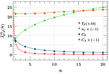
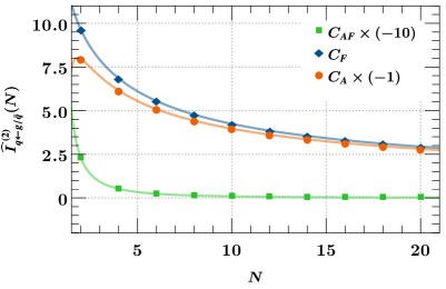
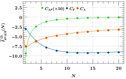
Figure 1: Two-loop non-logarithmic matching kernels for transverse-momentum resummation (upper line) and N-jettiness (lower line). Left: The contributions to the diagonal kernels $\widehat{I}_{q\leftarrow q}^{(2)}(N)$. Right: The same for the off-diagonal kernels $\widehat{I}_{q\leftarrow g}^{(2)}(N)$ and $\widehat{I}_{q\leftarrow\bar{q}}^{(2)}(N)$. The solid lines represent the analytical results from [2, 6], and the dots show the numbers of our automated approach. The numerical uncertainties of the latter are too small to be visible in the plots.

We start with transverse-momentum resummation, which is a SCET-2 observable and hence corresponds to the case $n=0$. According to the collinear-anomaly relation (14), we need to combine the bare beam-function matching kernels with the corresponding soft function that we obtain from SoftSERVE. Our results for the collinear-anomaly exponent $d_{2}$ are shown in Table 1, and the non-logarithmic terms of the Mellin-space matching kernels are displayed in the upper panels of Figure 1. The plots also show the analytic results from [2], and we observe a very good agreement with the numerical predictions of our novel automated approach.

We next consider the N-jettiness beam function, which is a SCET-1 observable with $n=1$. In this case we extract the two-loop non-cusp anomalous dimension $\gamma_{1}^{B}$ and the non-logarithmic terms of the matching kernels $\widehat{I}_{i\leftarrow j}^{(2)}(N)$. The former are given in Table 1, and the latter are displayed in the lower panels of Figure 1. Our numbers are again in excellent agreement with the known analytic results [6].

7 Conclusion

We have presented a novel framework to calculate beam functions at two-loop order for a broad class of observables. Our approach is based on suitable phase-space parametrisations and a systematic application of sector decomposition and non-linear transformations, which allows us to expose all phase-space singularities in an observable-independent fashion. In order to avoid distributions, we furthermore chose to work in the Mellin-Laplace space, but we emphasise that our approach is not limited to this assumption, and we in fact already started to explore a direct calculation in momentum space. Our method has been implemented in the public package pySecDec, and it has been validated against known results in the literature for transverse-momentum resummation and N-jettiness. As a further application, we recently calculated the quark beam function for jet-veto resummation [15]. In the future we plan to extend our setup to gluon beam functions as well as to publish an automated standalone C++ code in the spirit of SoftSERVE.

Acknowledgement

This work was supported by the Deutsche Forschungsgemeinschaft (DFG, German Research Foundation) under grant 396021762 - TRR 257 (“Particle Physics Phenomenology after the Higgs Discovery”).

References

- [1] S. Catani, L. Cieri, D. de Florian, G. Ferrera and M. Grazzini, Universality of transverse-momentum resummation and hard factors at the NNLO, Nucl. Phys. B 881 (2014) 414–443, [1311.1654].
- [2] T. Gehrmann, T. Luebbert and L. L. Yang, Calculation of the transverse parton distribution functions at next-to-next-to-leading order, JHEP 06 (2014) 155, [1403.6451].
- [3] M.-x. Luo, T.-Z. Yang, H. X. Zhu and Y. J. Zhu, Quark Transverse Parton Distribution at the Next-to-Next-to-Next-to-Leading Order, Phys. Rev. Lett. 124 (2020) 092001, [1912.05778].
- [4] M. A. Ebert, B. Mistlberger and G. Vita, Transverse momentum dependent PDFs at N3LO, JHEP 09 (2020) 146, [2006.05329].
- [5] M.-x. Luo, T.-Z. Yang, H. X. Zhu and Y. J. Zhu, Unpolarized quark and gluon TMD PDFs and FFs at N3LO, JHEP 06 (2021) 115, [2012.03256].
- [6] J. R. Gaunt, M. Stahlhofen and F. J. Tackmann, The Quark Beam Function at Two Loops, JHEP 04 (2014) 113, [1401.5478].
- [7] J. Gaunt, M. Stahlhofen and F. J. Tackmann, The Gluon Beam Function at Two Loops, JHEP 08 (2014) 020, [1405.1044].
- [8] A. Behring, K. Melnikov, R. Rietkerk, L. Tancredi and C. Wever, Quark beam function at next-to-next-to-next-to-leading order in perturbative QCD in the generalized large- approximation, Phys. Rev. D 100 (2019) 114034, [1910.10059].
- [9] M. A. Ebert, B. Mistlberger and G. Vita, -jettiness beam functions at N3LO, JHEP 09 (2020) 143, [2006.03056].
- [10] J. R. Gaunt and M. Stahlhofen, The Fully-Differential Quark Beam Function at NNLO, JHEP 12 (2014) 146, [1409.8281].
- [11] J. R. Gaunt and M. Stahlhofen, The fully-differential gluon beam function at NNLO, JHEP 07 (2020) 234, [2004.11915].
- [12] S. Gangal, J. R. Gaunt, M. Stahlhofen and F. J. Tackmann, Two-Loop Beam and Soft Functions for Rapidity-Dependent Jet Vetoes, JHEP 02 (2017) 026, [1608.01999].
- [13] S. Abreu, J. R. Gaunt, P. F. Monni, L. Rottoli and R. Szafron, Quark and gluon two-loop beam functions for leading-jet and slicing at NNLO, 2207.07037.
- [14] G. Bell, K. Brune, G. Das and M. Wald, Automation of Beam and Jet functions at NNLO, SciPost Phys. Proc. 7 (2022) 021, [2110.04804].
- [15] G. Bell, K. Brune, G. Das and M. Wald, The NNLO quark beam function for jet-veto resummation, 2207.05578.
- [16] G. Bell, R. Rahn and J. Talbert, Two-loop anomalous dimensions of generic dijet soft functions, Nucl. Phys. B 936 (2018) 520–541, [1805.12414].
- [17] G. Bell, R. Rahn and J. Talbert, Generic dijet soft functions at two-loop order: correlated emissions, JHEP 07 (2019) 101, [1812.08690].
- [18] G. Bell, R. Rahn and J. Talbert, Generic dijet soft functions at two-loop order: uncorrelated emissions, JHEP 09 (2020) 015, [2004.08396].
- [19] T. Becher and G. Bell, Analytic Regularization in Soft-Collinear Effective Theory, Phys. Lett. B 713 (2012) 41–46, [1112.3907].
- [20] D. A. Kosower and P. Uwer, One loop splitting amplitudes in gauge theory, Nucl. Phys. B 563 (1999) 477–505, [hep-ph/9903515].
- [21] Z. Bern, V. Del Duca, W. B. Kilgore and C. R. Schmidt, The infrared behavior of one loop QCD amplitudes at next-to-next-to leading order, Phys. Rev. D 60 (1999) 116001, [hep-ph/9903516].
- [22] G. F. R. Sborlini, D. de Florian and G. Rodrigo, Double collinear splitting amplitudes at next-to-leading order, JHEP 01 (2014) 018, [1310.6841].
- [23] J. M. Campbell and E. W. N. Glover, Double unresolved approximations to multiparton scattering amplitudes, Nucl. Phys. B 527 (1998) 264–288, [hep-ph/9710255].
- [24] S. Catani and M. Grazzini, Collinear factorization and splitting functions for next-to-next-to-leading order QCD calculations, Phys. Lett. B 446 (1999) 143–152, [hep-ph/9810389].
- [25] S. Borowka, G. Heinrich, S. Jahn, S. P. Jones, M. Kerner, J. Schlenk et al., pySecDec: a toolbox for the numerical evaluation of multi-scale integrals, Comput. Phys. Commun. 222 (2018) 313–326, [1703.09692].
- [26] T. Hahn, CUBA: A Library for multidimensional numerical integration, Comput. Phys. Commun. 168 (2005) 78–95, [hep-ph/0404043].
- [27] T. Becher and M. Neubert, Drell-Yan Production at Small , Transverse Parton Distributions and the Collinear Anomaly, Eur. Phys. J. C 71 (2011) 1665, [1007.4005].
- [28] T. Becher, G. Bell and M. Neubert, Factorization and Resummation for Jet Broadening, Phys. Lett. B 704 (2011) 276–283, [1104.4108].