Quantization enabled Privacy Protection in Decentralized Stochastic Optimization

Abstract

By enabling multiple agents to cooperatively solve a global optimization problem in the absence of a central coordinator, decentralized stochastic optimization is gaining increasing attention in areas as diverse as machine learning, control, and sensor networks. Since the associated data usually contain sensitive information, such as user locations and personal identities, privacy protection has emerged as a crucial need in the implementation of decentralized stochastic optimization. In this paper, we propose a decentralized stochastic optimization algorithm that is able to guarantee provable convergence accuracy even in the presence of aggressive quantization errors that are proportional to the amplitude of quantization inputs. The result applies to both convex and non-convex objective functions, and enables us to exploit aggressive quantization schemes to obfuscate shared information, and hence enables privacy protection without losing provable optimization accuracy. In fact, by using a stochastic ternary quantization scheme, which quantizes any value to three numerical levels, we achieve quantization-based rigorous differential privacy in decentralized stochastic optimization, which has not been reported before. In combination with the presented quantization scheme, the proposed algorithm ensures, for the first time, rigorous differential privacy in decentralized stochastic optimization without losing provable convergence accuracy. Simulation results for a distributed estimation problem as well as numerical experiments for decentralized learning on a benchmark machine learning dataset confirm the effectiveness of the proposed approach.

I Introduction

Initially introduced in the 1980s in the context of parallel and distributed computation [1, 2], decentralized optimization is finding increasing applications. For example, in sensor-network based acoustic-event localization, spatially distributed sensors multilaterate the position of a target event using individual sensors’ range measurements such as time-of-arrival or signal-strength-profile measurements [3]. Because the range measurements acquired by individual sensors are noisy, decentralized optimization is commonly employed for the network to cooperatively estimate the target position, particularly when the network is mobile or formed in an ad-hoc manner [3, 4]. Another example is the multi-robot rendezvous problem, where robots with different battery levels cooperatively determine a meeting time and place using decentralized optimization to minimize the total energy expenditure of the network [5]. In wide-area monitoring and control of power systems, decentralized optimization enables multiple local control centers in a large power system network to cooperatively estimate and further damp inter-area electro-mechanical oscillations, which is vital for power system stability [6]. In large-scale machine learning, decentralized optimization algorithms are becoming an important solution to parallelling both data and computation so as to handle the enormous growth in data and model sizes [7].

In decentralized optimization, participating agents interleave on-device computation and peer-to-peer communications to cooperatively solve a network optimization problem. In recent years, a particular type of decentralized optimization, i.e., decentralized stochastic optimization, in which participating agents use noisy local gradients for optimization, is gaining increased traction due to its superior performance in handling large or noisy data sets. For example, in modern machine learning applications on massive datasets, such stochastic optimization methods are highly preferred because they allow multiple devices to train a neural network model collectively using local noisy gradients calculated from a small batch of data points available to individual agents. Using a small batch of data points yields a noisy estimation of the exact gradient, but it is completely necessary because evaluating the precise gradient using all available data can be extremely expensive in computation or even practically infeasible. Furthermore, in the era of Internet of things which connect massive low-cost sensing and communication devices, the data fed to optimization computations are usually subject to measurement noises [8]. As deterministic (batch) optimization approaches typically falter when dealing with noisy data [9], investigating decentralized stochastic optimization algorithms becomes a mandatory task.

Although centralized stochastic optimization algorithms can date back to the 1950s [9], results on completely decentralized stochastic optimization in the absence of any coordinator only started to gain attention in the past decade. So far, plenty of decentralized stochastic optimization algorithms have been reported, both for convex objective functions (e.g., [10, 11, 12, 13, 14, 15, 16, 17]) and non-convex objective functions (e.g., [18, 19, 20, 21, 22, 23]). In these decentralized stochastic optimization algorithms, because participating agents only share gradients/model updates and do not let raw data leave participants’ machines, these algorithms were believed to be able to protect the privacy of participating agents. However, recent studies tell a completely different story: not only can an adversary reversely infer the properties (e.g., membership associations) of the data used in optimization [24, 25], an adversary can even precisely infer raw data used in optimization from shared gradients (pixel-wise accurate for images and token-wise matching for texts) [26]. These information leakages pose a severe threat to the privacy of participating agents in decentralized stochastic optimization, as the data involved in optimization computation often contain sensitive information such as medical records and financial transactions.

Compared with centralized optimization or distributed optimization with a coordinator, privacy protection in completely decentralized optimization is much more challenging due to the lack of a trusted party. In fact, in decentralized stochastic optimization, no participating agents are trustworthy as every participating agent can use received messages to infer other participating agents’ sensitive information. Recently, results have been reported to address the privacy issue in decentralized stochastic optimization. One approach is to employ secure multi-party computation approaches such as homomorphic encryption [27] or garbled circuit [28]. However, while allowing exact computations, these approaches are very heavy in computation/communication overhead, usually incurring a runtime overhead of three to four orders of magnitude [29]. Furthermore, except our prior results [24, 30], most existing homomorphic encryption based privacy approaches employ a server (e.g., in [31, 32, 33]), which does not exist in completely decentralized optimization. Hardware based privacy approaches such as trusted hardware enclaves have also been reported [29]. However, similar to homomorphic encryption based approaches, these approaches cannot be directly used to prevent multiple data providers from inferring each others’ data during decentralized stochastic optimization. Another commonly used approach to enable privacy in decentralized optimization is differential privacy, which adds uncorrelated noise to shared gradients/model updates (e.g., [34, 35, 36, 37]). However, these uncorrelated-noise based approaches are subject to a fundamental trade-off between enabled privacy and optimization accuracy [38], i.e. a stronger privacy protection requires a greater magnitude of uncorrelated noise, which will unavoidably leads to a more intense reduction in optimization accuracy. Recently, results were reported to enable privacy by exploiting the structural properties of decentralized optimization [39, 40, 41]. For example, the authors in [40, 41] proposed to add a constant uncertain parameter in projection or step sizes to enable privacy protection. The authors of [42] proposed to judiciously construct spatially correlated “structured” noise to cover gradient information without compromising optimization accuracy. However, the privacy protection enabled by these approaches is restricted: projection based privacy depends on the size of the projection set – a large projection set nullifies privacy protection whereas a small projection set offers strong privacy protection but requires a priori knowledge of the optimal solution; “structured” noise based approaches require each agent to have a certain number of neighbors whose shared messages are inaccessible to the adversary. In fact, such a constraint on information accessible to the adversary is required in most existing accuracy-maintaining privacy solutions to decentralized optimization. For example, our studies in [24] show that even partially homomorphic encryption based privacy approaches require the adversary not to have access to all messages shared by a target agent. One exception is our recent work [43, 44], which injects stochasticity in stepsizes and can enable privacy protection even when adversaries have access to all shared messages in the network.

In this paper, we propose to leverage aggressive quantization effects to enable strong privacy protection in decentralized stochastic optimization without compromising optimization accuracy. More specifically, we propose a decentralized stochastic optimization algorithm that can ensure provable convergence accuracy under aggressive quantization effects. This decentralized stochastic optimization algorithm allows us to quantize any shared value to three numerical levels and hence obfuscate exchanged messages without compromising optimization accuracy. In fact, we rigorously prove that the quantization scheme can enable a strict $(0,\delta)-$differential privacy for participating agents’ gradient information, which has not been reported in the literature. The ability to use this aggressive quantization scheme also allows us to significantly reduce communication overhead without losing optimization accuracy since each real-valued message becomes representable with two bits after quantization.

The main contributions of the paper are as follows: 1) We propose a completely decentralized stochastic optimization algorithm that can maintain provable optimization accuracy in the presence of aggressive quantization errors that can be proportional to the norm of input values. This is different from existing results that require the quantization errors to be bounded [45] or diminishing [46] with time. Furthermore, we obtain provable convergence for both convex objective functions and non-convex objective functions, which is different from [47] which only addresses strongly convex objective functions; 2) We propose to use a stochastic ternary quantization scheme to achieve rigorous $(0,\delta)-$differential privacy, which has not been reported in the literature. Note that $(0,\delta)-$differential privacy is stronger than the commonly used $(\epsilon,\delta)-$differential privacy; 3) By integrating with ternary quantization, our algorithm achieves rigorous $(0,\delta)-$differential privacy under provable convergence accuracy. To the best of our knowledge, this is the first time both rigorous $(0,\delta)-$differential privacy and provable convergence accuracy are achieved simultaneously in decentralized stochastic optimization; 4) The ternary quantization scheme also enables us to improve communication efficiency, which is crucial in scenarios where the communication bandwidth is limited.

The paper is organized as follows: Sec. II provides the problem formulation. Sec. III presents the decentralized stochastic optimization algorithm. Sec. IV proves converge of all agents to the same stationary point in the presence of aggressive quantization effects when the objective functions are non-convex. Sec. V proves that the proposed algorithm guarantees convergence of all agents to the optimal solution in the presence of aggressive quantization effects when the objective functions are convex. Sec. VI proves that a specific instantiation of allowable quantization schemes can enable rigorous $(0,\delta)-$differential privacy and, hence the proposed algorithm can achieve rigorous $(0,\delta)-$differential privacy with provable convergence accuracy. Sec. VII gives simulation results as well as numerical experiments on a benchmark machine learning dataset to confirm the obtained results. Finally Sec. VIII concludes the paper.

Notation: We use the symbol $\mathbb{R}$ to denote the set of real numbers and $\mathbb{R}^{d}$ the Euclidean space of dimension $d$. ${\bf 1}$ denotes a column vector of appropriate dimension with all entries equal to 1. A vector is viewed as a column vector, unless otherwise stated. For a vector $x$, $x_{i}$ denotes its $i$th element. $A^{T}$ denotes the transpose of matrix $A$ and $x^{T}y$ denotes the scalar product of two vectors $x$ and $y$. We use $\langle\cdot\rangle$ to denote inner product and $\|\cdot\|$ to denote the standard Euclidean norm $\|x\|=\sqrt{x^{T}x}$. We use $\|\cdot\|_{1}$ and $\|\cdot\|_{\infty}$ to denote the $\ell_{1}$ norm $\|x\|_{1}=\sum_{i=1}^{d}|x_{i}|$ and the $\ell_{\infty}$ norm $\|x\|_{\infty}=\max(|x_{1}|,|x_{2}|,\cdots,|x_{d}|)$, respectively. A square matrix $A$ is said to be column-stochastic when its elements in every column add up to one. A matrix $A$ is said to be doubly-stochastic when both $A$ and $A^{T}$ are column-stochastic matrices. We use $P(\mathcal{A})$ to denote the probability of an event $\mathcal{A}$ and $\mathbb{E}\left[x\right]$ the expected value of a random variable $x$.

II Problem Formulation

We consider a network of $m$ agents solving the following optimization problem cooperatively:

$$\min\limits_{x\in\mathbb{R}^{d}}\frac{1}{m}\sum_{i=1}^{m}f_{i}(x),\quad f_{i}(x)\triangleq\mathbb{E}_{\xi_{i}\sim\mathcal{D}_{i}}\left[F_{i}(x,\xi_{i})\right]$$ (1)

where $x\in\mathbb{R}^{d}$ is the optimization variable common to all agents but $F_{i}:\mathbb{R}^{d}\times\mathbb{R}\rightarrow\mathbb{R}$ is a local stochastic loss function private to agent $i$. $\mathcal{D}_{i}$ is the local distribution of data samples. In practice, the distribution $\mathcal{D}_{i}$ is usually unknown and we only have access to $n_{i}$ realizations of it, denoted by $\xi_{i,1},\xi_{i,2},\cdots,\xi_{i,n_{i}}$, where $\xi_{i,j}$ denotes the $j$th random data sample of node $i$. Thus $f_{i}(x)$ in (1) is usually determined by $f_{i}(x)=\frac{1}{n_{i}}\sum_{j=1}^{n_{i}}F_{i}(x,\xi_{i,j})$ which makes (1) the empirical risk minimization problem.

Because of the randomness in $F_{i}(x,\xi_{i})$, the gradient that each agent $i$ can obtain is subject to noises. We denote the gradient that agent $i$ obtains at iteration $k$ for optimization as $g_{i}^{k}(x,\xi_{i})$, which will hereafter be abbreviated as $g_{i}^{k}$. We make the following standard assumption about $f_{i}(\cdot)$ and $g_{i}^{k}$:

Assumption 1.

1. All $f_{i}(\cdot)$ are Lipschitz continuous with Lipschitz gradients

   $$\|\nabla f_{i}(x)-\nabla f_{i}(y)\|\leq L\|x-y\|,\>\forall x\in\mathbb{R}^{d},y\in\mathbb{R}^{d},$$

   and (1) always has at least one optimal solution $x^{\ast}$, i.e., $\sum_{i=1}^{m}\nabla f_{i}(x^{\ast})=0$;

2. All $g_{i}^{k}$ satisfy

   $$\mathbb{E}_{\xi_{i}\backsim\mathcal{D}_{i}}\left[g_{i}^{k}\right]=\nabla f_{i}(x_{i}^{k}),\>\forall i$$

   $$\mathbb{E}_{\xi_{i}\backsim\mathcal{D}_{i}}\left[\|g_{i}^{k}-\nabla f_{i}(x)\|^{2}\right]\leq\sigma^{2},\>\forall i,x$$

In order for the network of $m$ agents to cooperatively solve (1) in a decentralized manner, we assume that the $m$ agents interact on an undirected graph. The interaction can be described by a weight matrix $W$. More specifically, if agent $i$ and agent $j$ can communicate and interact with each other, then the $(i,j)$th entry of $W$, i.e., $w_{ij}$, is positive. Otherwise, $w_{ij}$ is zero. The neighbor set $\mathcal{N}_{i}$ of agent $i$ is defined as the set of agents satisfying $\{j|w_{ij}>0\}$. We define a diagonal matrix $D$ with the $i$th diagonal entry determined as $d_{ii}=\sum_{j\in{\mathbb{N}}_{i}}w_{ij}$. So the matrix $D-W$ will be the commonly referred graph Laplacian matrix. To ensure that the network can cooperatively solve (1), we make the following standard assumption about the interaction:

Assumption 2.

The interaction topology forms an undirected connected network, i.e., the second smallest eigenvalue $\rho$ of the graph Laplacian matrix $L_{w}\triangleq D-W$ is positive.

In decentralized stochastic optimization, gradients are directly computed from raw data and hence embed sensitive information. For example, in decentralized-optimization based localization, disclosing the gradient of an agent amounts to disclosing its position [24, 35]. In machine learning applications, gradients are directly calculated from and embed information of sensitive training data [26]. Therefore, in this paper, we define privacy as preventing agents’ gradients from being inferable by adversaries.

We consider two potential adversaries in decentralized stochastic optimization, which are the two most commonly used models of attacks in privacy research [48] and have been widely used in the control community [49, 50]:

• Honest-but-curious attacks are attacks in which a participating agent or multiple participating agents (colluding or not) follows all protocol steps correctly but is curious and collects all received intermediate data in an attempt to learn the sensitive information about other participating agents.

• Eavesdropping attacks are attacks in which an external eavesdropper wiretaps all communication channels to intercept exchanged messages so as to learn sensitive information about sending agents.

An honest-but-curious adversary (e.g., agent $i$) has access to the internal state $x_{i}^{k}$, which is unavailable to external eavesdroppers. However, an eavesdropper has access to all shared information in the network, whereas an honest-but-curious agent can only access shared information that is destined to it.

In this paper, we propose to leverage quantization effects to enable differential privacy in decentralized stochastic optimization. We adopt the definition of ($\epsilon,\delta$)-differential privacy following standard conventions [38]:

Definition 1.

For a randomized function $h(x)$, we say that it is $(\epsilon,\delta)$-differentially private if for all subsets $S$ of the image set of the function $h(x)$ and for all $x,y$ with $\|x-y\|_{1}\leq 1$, we always have

$$P(h(x)\in S)\leq e^{\epsilon}P(h(y)\in S)+\delta.$$

Definition 1 says that for two inputs $x$ and $y$ with $\ell_{1}$-norm difference no more than $1$, a mechanism $h(\cdot)$ achieves $(\epsilon,\delta)-$differential privacy if it can ensure that the outputs of the two inputs are different in probabilities by at most $\epsilon$ and $\delta$ specified on the right hand side of the above inequality. Clearly, a smaller $\epsilon\geq 0$ or $\delta\geq 0$ means better differential-privacy protection. In Sec. VI we will prove that a specific quantization mechanism can enable $(0,\delta)-$differential privacy protection for exchanged information. Note that under a fixed value of $\delta$, $(0,\delta)-$differential privacy is stronger than $(\epsilon,\delta)-$differential privacy for any $\epsilon>0$.

Remark 1.

In the original definition of differential privacy in [38, 51], because the input space is discrete, i.e., $x$ and $y$ are strings, the distance between $x$ and $y$ is measured by the number of positions at which the corresponding symbols are different (Hamming distance). In our case, since the input space is continuous, we use $\ell_{1}$ norm to measure the distance between two real vectors $x$ and $y$. In fact, any $\ell_{p}$ norm defined by $\|x\|_{p}=\left(|x_{1}|^{p}+|x_{2}|^{p}+\cdots+|x_{m}|^{p}\right)^{1/p}$ with $p\geq 1$ can be used in the definition.

III Quantization-enabled privacy-preserving decentralized optimization algorithm

  Algorithm 1: Quantization-enabled Privacy-preserving Decentralized Stochastic Optimization

 

1. Public parameters: $W$, $\epsilon^{k}$, $\lambda^{k}$ $x_{i}^{0}=0$ for all $i$, the total number of iterations $t$

2. For the $i$th agent, at iteration $k$

   1. Determine local gradient $g_{i}^{k}$;

   2. Determine quantized state $\mathcal{Q}(x_{i}^{k})$ and send it to all agents $j\in\mathbb{N}_{i}$;

   3. After receiving $\mathcal{Q}(x_{j}^{k})$ from all $j\in\mathbb{N}_{i}$, update state as

      $$x_{i}^{k+1} =x_{i}^{k}+\epsilon^{k}\sum_{j\in\mathbb{N}_{i}}w_{ij}(\mathcal{Q}(x_{j}^{k})-\mathcal{Q}(x_{i}^{k}))-\epsilon^{k}\lambda^{k}g_{i}^{k}$$

3. end

 

Before presenting our quantization-enabled privacy-preserving approach for decentralized stochastic optimization, we first discuss why conventional decentralized stochastic optimization algorithms leak gradient information of participating agents.

By assigning a copy $x_{i}$ of the decision variable $x$ to each agent $i$, and then imposing the requirement $x_{i}=x$ for all $1\leq i\leq m$, we can rewrite the optimization problem (1) in the following form [52]:

$$\min\limits_{x\in\mathbb{R}^{md}}f(x)=\frac{1}{m}\sum_{i=1}^{m}f_{i}(x_{i})\quad{\rm s.t.}\quad x_{1}=x_{2}=\cdots=x_{m}$$ (2)

where $x=[x_{1}^{T},x_{2}^{T},\cdots,x_{m}^{T}]^{T}$. Conventional decentralized optimization algorithms usually take the following form [7, 20]:

$$x_{i}^{k+1}=x_{i}^{k}+\sum_{j\in\mathbb{N}_{i}}w_{ij}(x_{j}^{k}-x_{i}^{k})-\eta g_{i}^{k}$$

where $x_{i}^{k}$ denotes the optimization variable maintained by agent $i$ at iteration $k$, and $\eta$ denotes the optimization stepsize, which should be no greater than $\frac{1}{L}$ to ensure stability [20]. Because $w_{ij}$ has to be publicly known to establish conditions in Assumption 2 in a decentralized manner [53] and agent $i$ shares $x_{i}^{k}$ with all its neighbors, an adversary can calculate the gradient $g_{i}^{k}$ of any agent based on publicly known $W$ and $\eta$ if it has access to all information shared in the network.

Motivated by this observation, we propose the following decentralized optimization algorithm which leverages quantization to enable privacy protection:

$$x_{i}^{k+1} =x_{i}^{k}+\epsilon^{k}\sum_{j\in\mathbb{N}_{i}}w_{ij}\left(\mathcal{Q}(x_{j}^{k})-\mathcal{Q}(x_{i}^{k})\right)-\epsilon^{k}\lambda^{k}g_{i}^{k}$$ (3)

where $\lambda^{k}$ and $\epsilon^{k}$ are publicly-known design parameters crucial for ensuring provable convergence accuracy under aggressive quantization effects, and their design will be elaborated on later. Note that, although agent $i$ has access to $x_{i}^{k}$, we still use a quantized version of $x_{i}^{k}$ in the comparison term $\mathcal{Q}(x_{j}^{k})-\mathcal{Q}(x_{i}^{k})$ in (3). This is intuitive as when $x_{i}^{k}$ and $x_{j}^{k}$ are the same, we do not want the quantization operation to introduce an extra non-zero input to the optimization process. In fact, as shown in later derivations, this strategy will also simplify the evolution of the average optimization variable across all agents.

In our proposed algorithm (3), at iteration $k$, every agent $i$ only shares quantized state $x_{i}^{k}$ (see details in Algorithm 1). Therefore, even if an adversary has access to the quantized state of an agent $i$ as well as all information received by agent $i$ (which are also quantized), the adversary still cannot use the dynamics (3) to precisely infer the gradient of agent $i$ due to quantization induced errors. In fact, as will be proved later, the proposed algorithm can have provable convergence even in the presence of aggressive quantization schemes with large quantization errors, which will enable us to achieve strict $(0,\delta)$-differential privacy protection for all participating agents. More specifically, we consider stochastic quantization schemes satisfying the following Assumption:

Assumption 3.

The quantizer $\mathcal{Q}(\cdot)$ is unbiased and its variance is proportionally bounded by the input’s norm, i.e., $\mathbb{E}\left[\mathcal{Q}(x)|x\right]=x$ and $\mathbb{E}\left[\|\mathcal{Q}(x)-x\|^{2}|x\right]\leq\beta\|x\|^{2}$ hold for some constant $\beta$ and any $x$. And the quantization on different agents are independent of each other.

Remark 2.

Note that the quantization schemes considered in Assumption 3 are quite general and include the commonly used error-bounded quantization schemes (in, e.g., [54, 55, 45]) and error-diminishing quantization schemes (in, e.g., [56, 46]) as special cases.

Remark 3.

Note that when the quantization scheme is designed such that it only outputs the sign of the quantization input (which still satisfies the conditions in Assumption 3), the inter-agent coupling in the proposed algorithm looks similar to the interaction in existing decentralized optimization algorithms that use only the sign of relative states (see, [57, 58]). However, there is a crucial difference between the two in that the quantization scheme here can be implemented by every participating agent without knowing anything about its neighbors’ states, whereas the relative-state sign based interaction (which arises in other contexts) requires an agent to know (some) information about its neighbors’ states.

Augmenting the decision variables of all agents as $x^{k}=[(x_{1}^{k})^{T},(x_{2}^{k})^{T},\cdots,(x_{m}^{k})^{T}]^{T}$, we can write the overall network dynamics of the proposed decentralized optimization algorithm as follows

$$x^{k+1}=(A^{k}\otimes I_{d})x^{k}-\epsilon^{k}\lambda^{k}g^{k}-\epsilon^{k}(L_{w}\otimes I_{d})V^{k}$$ (4)

where $L_{w}$ is the Laplacian matrix defined in Assumption 2,

$$A^{k}=(I-\epsilon^{k}L)\in\mathbb{R}^{m\times m},$$

$$g^{k}=\left[(g_{1}^{k})^{T},\,(g_{2}^{k})^{T},\,\cdots,(g_{m}^{k})^{T}\right]^{T}\in\mathbb{R}^{md\times 1},$$

$$V^{k}=\left[(v_{1}^{k})^{T},\,(v_{2}^{k})^{T},\,\cdots,(v_{m}^{k})^{T}\right]^{T}\in\mathbb{R}^{md\times 1},$$

$$v_{i}^{k}=\mathcal{Q}(x_{i}^{k})-x_{i}^{k}\in\mathbb{R}^{d\times 1}$$

Here $\otimes$ denotes Kronecker product and $I_{d}$ denotes identity matrix of dimension $d$.

It can be obtained that the evolution of the average optimization variable $\bar{x}^{k}=\frac{\sum_{i=1}^{m}x_{i}^{k}}{m}$ follows

$$\bar{x}^{k+1} =\bar{x}^{k}+\frac{\epsilon^{k}}{m}\sum_{i=1}^{m}\sum_{j\in\mathbb{N}_{i}}w_{ij}\left(\mathcal{Q}(x_{j}^{k})-\mathcal{Q}(x_{i}^{k})\right)$$ (5)

$$\qquad\qquad\qquad\qquad\qquad\qquad-\epsilon^{k}\lambda^{k}\frac{\sum_{i=1}^{m}g_{i}^{k}}{m}$$

$$=\bar{x}_{i}^{k}-\epsilon^{k}\lambda^{k}\frac{\sum_{i=1}^{m}g_{i}^{k}}{m}$$

which is independent of the quantization error. Note that in the second equality, we used the fact that the network is undirected, i.e., $w_{ij}=w_{ji}$ from Assumption 2, which leads to the annihilation of all coupling terms due to $w_{ij}\left(\mathcal{Q}(x_{j}^{k})-\mathcal{Q}(x_{i}^{k})\right)+w_{ji}\left(\mathcal{Q}(x_{i}^{k})-\mathcal{Q}(x_{j}^{k})\right)=0$. This shows the benefit for agent $i$ to use its quantized state $x_{i}^{k}$ in the comparison term $\mathcal{Q}(x_{j}^{k})-\mathcal{Q}(x_{i}^{k})$ on the right hand side of (3).

Remark 4.

From the above argument, it can be seen that agents being able to update in a synchronized manner is key to guaranteeing the average optimization variable $\bar{x}^{k}$ to be immune to aggressive quantization errors.

In the following two sections, we will show that the proposed decentralized stochastic optimization algorithm still has provable convergence accuracy under aggressive quantization effects. More specifically, in Sec. IV, we will show that in the non-convex case, the algorithm guarantees provable convergence of all agents to the same stationary point; in Sec. V, we will show that in the convex case, the algorithm guarantees the convergence of all agents to the optimal solution.

IV Convergence Analysis In the Non-convex Case

In this section, we show that the proposed algorithm will ensure convergence of all agents to the same stationary point when the objective functions are non-convex, even under aggressive quantization effects.

To this end, we first show that when $\epsilon^{k}$ and $\lambda^{k}$ are chosen appropriately, $\|g_{i}^{k}\|$ and $\mathbb{E}\left[\|x^{k}\|^{2}\right]$ will always be bounded, which allows us to quantify the effects of quantization on the optimization process (note that here the expectation is taken with respect to the randomness in stochastic gradients and quantization up until iteration $k-1$). It is worth noting that as the results are obtained irrespective of the convexity of objective functions, they are applicable to the derivations in the convex case in the next section, too.

Lemma 1.

Under Assumption 1, the gradient $\|g_{i}^{k}\|$ is always bounded by some constant $G$.

Proof.

Under the conditions in Assumption 1, the result can be easily obtained from [23] or Lemma 3.3 in [59]. ∎

Lemma 2.

Under Assumption 1, Assumption 2, and Assumption 3, $\mathbb{E}\left[\|x^{k}\|^{2}\right]$ will always be bounded if the positive sequences $\epsilon^{k}$ and $\lambda^{k}$ satisfy $\sum_{k=1}^{\infty}(\epsilon^{k})^{2}<\infty$ and $\sum_{k=1}^{\infty}\epsilon^{k}(\lambda^{k})^{2}<\infty$, where the expectation is taken with respect to the randomness in stochastic gradients and quantization up until iteration $k-1$.

Proof.

The proof is given in Appendix B. ∎

Using Lemma 2, we can further obtain that the optimization variables $x_{i}^{k}$ of different agents will converge to the average optimization variable across all agents $\bar{x}^{k}$:

Lemma 3.

Under the conditions in Lemma 2, the proposed algorithm guarantees

$$\lim_{k\rightarrow\infty}\mathbb{E}\left[\|x^{k+1}-\hat{\bar{x}}^{k+1}\|^{2}\right]=0$$

where $\hat{\bar{x}}^{k}\triangleq{\bf 1}_{m}\otimes\bar{x}^{k}$ with ${\bf 1}_{m}$ denoting the $m$ dimensional column vector of $1$s. More specifically, represent the decaying rate of $\lambda^{k}$ and $\epsilon^{k}$ as $0<\delta_{1}<1$ and $0<\delta_{2}<1$, respectively, i.e., there exist some positive $a_{1}$, $a_{2}$, and $a_{3}$ such that $\lambda^{k}\leq\frac{a_{1}}{(a_{3}k+1)^{\delta_{1}}}$ and $\epsilon^{k}\leq\frac{a_{2}}{(a_{3}k+1)^{\delta_{2}}}$ hold, then we have

$$\lim_{k\rightarrow\infty}(1+k)^{\delta}\mathbb{E}\left[\|x^{k+1}-\hat{\bar{x}}^{k+1}\|^{2}\right]=0$$

for any $0\leq\delta<\min\{2\delta_{1},\delta_{2}\}$.

Proof.

The proof is given in Appendix C. ∎

Based on these results, we can prove the following results on the convergence of all agents to the same stationary point where the gradients are zero:

Theorem 1.

Under Assumptions 1, 2, and 3, when the sequences $\epsilon^{k}$ and $\lambda^{k}$ are selected such that the sequence $\epsilon^{k}\lambda^{k}$ is not summable, but $(\epsilon^{k})^{2}$ and $\epsilon^{k}(\lambda^{k})^{2}$ are summable, i.e.,

$$\sum_{k=1}^{\infty}\epsilon^{k}\lambda^{k}=+\infty,\>\>\sum_{k=1}^{\infty}(\epsilon^{k})^{2}<\infty,\>\>\sum_{k=1}^{\infty}\epsilon^{k}(\lambda^{k})^{2}<\infty$$ (6)

then the proposed algorithm will guarantee the following results:

$$\lim_{t\rightarrow\infty}\frac{\sum_{k=0}^{t}\epsilon^{k}\lambda^{k}\mathbb{E}\left[\left\|\nabla f(\bar{x}^{k})\right\|^{2}\right]}{\sum_{k=0}^{t}\epsilon^{k}\lambda^{k}}=0,$$ (7)

$$\lim_{t\rightarrow\infty}\frac{\sum_{k=0}^{t}\epsilon^{k}\lambda^{k}\mathbb{E}\left[\left\|\frac{\sum_{i=1}^{m}\nabla f_{i}(x_{i}^{k})}{m}\right\|^{2}\right]}{\sum_{k=0}^{t}\epsilon^{k}\lambda^{k}}=0$$

where the expectation is taken with respect to the randomness in stochastic gradients and quantization up until iteration $k-1$.

Proof.

From the Lipschitz gradient condition in Assumption 1, we have

$$f(y)\leq f(x)+\langle\nabla f(x),y-x\rangle+\frac{L\|y-x\|^{2}}{2}$$

for any $x\in\mathbb{R}^{d}$ and $y\in\mathbb{R}^{d}$. By plugging $y=\bar{x}^{k+1}$ and $x=\bar{x}^{k}$ into the above inequality, we can have the following relationship based on (5):

$$f(\bar{x}^{k+1}) \leq f(\bar{x}^{k})+\left\langle\nabla f(\bar{x}^{k}),-\epsilon^{k}\lambda^{k}\frac{\sum_{i=1}^{m}g_{i}^{k}}{m}\right\rangle$$ (8)

$$\qquad+\frac{L}{2}\left\|-\epsilon^{k}\lambda^{k}\frac{\sum_{i=1}^{m}g_{i}^{k}}{m}\right\|^{2}$$

Taking expectation on both sides, we can obtain

$$\mathbb{E}\left[f(\bar{x}^{k+1})\right]$$ (9)

$$\leq\mathbb{E}\left[f(\bar{x}^{k})\right]+\mathbb{E}\left[\left\langle\nabla f(\bar{x}^{k}),-\epsilon^{k}\lambda^{k}\frac{\sum_{i=1}^{m}g_{i}^{k}}{m}\right\rangle\right]$$

$$\qquad+\frac{L}{2}\mathbb{E}\left[\left\|-\epsilon^{k}\lambda^{k}\frac{\sum_{i=1}^{m}g_{i}^{k}}{m}\right\|^{2}\right]$$

$$=\mathbb{E}\left[f(\bar{x}^{k})\right]-\epsilon^{k}\lambda^{k}\mathbb{E}\left[\left\langle\nabla f(\bar{x}^{k}),\frac{\sum_{i=1}^{m}g_{i}^{k}}{m}\right\rangle\right]$$

$$\qquad+\frac{L(\epsilon^{k}\lambda^{k})^{2}}{2m^{2}}\mathbb{E}\left[\left\|-\sum_{i=1}^{m}g_{i}^{k}\right\|^{2}\right]$$

Using the equality $2\langle X,Y\rangle=\|X\|^{2}+\|Y\|^{2}-\|X-Y\|^{2}$, we arrive at the following relationship for the second term on the right hand side of (9):

$$\mathbb{E}\left[\left\langle\nabla f(\bar{x}^{k}),\frac{\sum_{i=1}^{m}g_{i}^{k}}{m}\right\rangle\right]$$ (10)

$$=\mathbb{E}\left[\left\langle\nabla f(\bar{x}^{k}),\frac{\sum_{i=1}^{m}\nabla f_{i}(x_{i}^{k})}{m}\right\rangle\right]$$

$$=\frac{1}{2}\mathbb{E}\left[\left\|\nabla f(\bar{x}^{k})\right\|^{2}\right]+\frac{1}{2}\mathbb{E}\left[\left\|\frac{\sum_{i=1}^{m}\nabla f_{i}(x_{i}^{k})}{m}\right\|^{2}\right]$$

$$\qquad-\frac{1}{2}\mathbb{E}\left[\left\|\nabla f(\bar{x}^{k})-\frac{\sum_{i=1}^{m}\nabla f_{i}(x_{i}^{k})}{m}\right\|^{2}\right]$$

$$\geq\frac{1}{2}\mathbb{E}\left[\left\|\nabla f(\bar{x}^{k})\right\|^{2}\right]+\frac{1}{2}\mathbb{E}\left[\left\|\frac{\sum_{i=1}^{m}\nabla f_{i}(x_{i}^{k})}{m}\right\|^{2}\right]$$

$$\qquad-\frac{L^{2}}{2m}\sum_{i=1}^{m}\mathbb{E}\left[\left\|\bar{x}^{k}-x_{i}^{k}\right\|^{2}\right]$$

where we used the Lipschitz gradient assumption in Assumption 1 and the relationship $\|y_{1}+y_{2}+\cdots+y_{m}\|^{2}\leq m\sum_{i=1}^{m}\|y_{i}\|^{2}$ in the inequality.

For the third term on the right hand side of (9), we can bound it using the result that $g_{i}^{k}$ is bounded by $G$ obtained in Lemma 1:

$$\frac{L(\epsilon^{k}\lambda^{k})^{2}}{2m^{2}}\mathbb{E}\left[\left\|-\sum_{i=1}^{m}g_{i}^{k}\right\|^{2}\right] \leq\frac{L(\epsilon^{k}\lambda^{k})^{2}}{2m}\mathbb{E}\left[\sum_{i=1}^{m}\left\|g_{i}^{k}\right\|^{2}\right]$$ (11)

$$\leq\frac{LG^{2}(\epsilon^{k}\lambda^{k})^{2}}{2}$$

Plugging (10) and (11) into (9) leads to

$$\mathbb{E}\left[f(\bar{x}^{k+1})\right] \leq\mathbb{E}\left[f(\bar{x}^{k})\right]-\frac{1}{2}\epsilon^{k}\lambda^{k}\mathbb{E}\left[\left\|\nabla f(\bar{x}^{k})\right\|^{2}\right]$$ (12)

$$\quad-\frac{1}{2}\epsilon^{k}\lambda^{k}\mathbb{E}\left[\left\|\frac{\sum_{i=1}^{m}\nabla f_{i}(x_{i}^{k})}{m}\right\|^{2}\right]$$

$$\quad+\epsilon^{k}\lambda^{k}\frac{L^{2}}{2m}\sum_{i=1}^{m}\mathbb{E}\left[\left\|\bar{x}^{k}-x_{i}^{k}\right\|^{2}\right]$$

$$\quad+\frac{LG^{2}(\epsilon^{k}\lambda^{k})^{2}}{2}$$

or

$$\epsilon^{k}\lambda^{k}\mathbb{E}\left[\left\|\nabla f(\bar{x}^{k})\right\|^{2}\right]+\epsilon^{k}\lambda^{k}\mathbb{E}\left[\left\|\frac{\sum_{i=1}^{m}\nabla f_{i}(x_{i}^{k})}{m}\right\|^{2}\right]$$ (13)

$$\leq 2\left(\mathbb{E}\left[f(\bar{x}^{k})\right]-\mathbb{E}\left[f(\bar{x}^{k+1})\right]\right)$$

$$\quad+\epsilon^{k}\lambda^{k}\frac{L^{2}}{m}\sum_{i=1}^{m}\mathbb{E}\left[\left\|\bar{x}^{k}-x_{i}^{k}\right\|^{2}\right]+LG^{2}(\epsilon^{k}\lambda^{k})^{2}$$

Iterating the above inequality from $k=0$ to $k=t$ yields

$$\sum_{k=0}^{t} \left(\epsilon^{k}\lambda^{k}\mathbb{E}\left[\left\|\nabla f(\bar{x}^{k})\right\|^{2}\right]+\epsilon^{k}\lambda^{k}\mathbb{E}\left[\left\|\frac{\sum_{i=1}^{m}\nabla f_{i}(x_{i}^{k})}{m}\right\|^{2}\right]\right)$$ (14)

$$\leq 2\left(\mathbb{E}\left[f(\bar{x}^{0})\right]-\mathbb{E}\left[f(\bar{x}^{t+1})\right]\right)$$

$$\quad+\sum_{k=0}^{t}\epsilon^{k}\lambda^{k}\frac{L^{2}}{m}\sum_{i=1}^{m}\mathbb{E}\left[\left\|\bar{x}^{k}-x_{i}^{k}\right\|^{2}\right]$$

$$\quad+\sum_{k=0}^{t}LG^{2}(\epsilon^{k}\lambda^{k})^{2}$$

i.e.,

$$\frac{\sum_{k=0}^{t}\epsilon^{k}\lambda^{k}\mathbb{E}\left[\left\|\nabla f(\bar{x}^{k})\right\|^{2}\right]}{\sum_{k=0}^{t}\epsilon^{k}\lambda^{k}}$$ (15)

$$\qquad+\frac{\sum_{k=0}^{t}\epsilon^{k}\lambda^{k}\mathbb{E}\left[\left\|\frac{\sum_{i=1}^{m}\nabla f_{i}(x_{i}^{k})}{m}\right\|^{2}\right]}{\sum_{k=0}^{t}\epsilon^{k}\lambda^{k}}$$

$$\leq\frac{2\left(\mathbb{E}\left[f(\bar{x}^{0})\right]-\mathbb{E}\left[f(\bar{x}^{t+1})\right]\right)}{\sum_{k=0}^{t}\epsilon^{k}\lambda^{k}}$$

$$\qquad+\frac{\sum_{k=0}^{t}\epsilon^{k}\lambda^{k}\frac{L^{2}}{m}\sum_{i=1}^{m}\mathbb{E}\left[\left\|\bar{x}^{k}-x_{i}^{k}\right\|^{2}\right]}{\sum_{k=0}^{t}\epsilon^{k}\lambda^{k}}$$

$$\qquad+\frac{\sum_{k=0}^{t}LG^{2}(\epsilon^{k}\lambda^{k})^{2}}{\sum_{k=0}^{t}\epsilon^{k}\lambda^{k}}$$

It can be verified that when $\epsilon^{k}$ and $\lambda^{k}$ are selected in such a way that the conditions in (6) are satisfied, then the conditions in Lemma 3 will also be satisfied, which means that $\mathbb{E}\left[\left\|\bar{x}^{k}-x_{i}^{k}\right\|^{2}\right]$ will be in the same order as $(\lambda^{k})^{2}$ or $\epsilon^{k}$. This means that $\epsilon^{k}\lambda^{k}\frac{L^{2}}{m}\sum_{i=1}^{m}\mathbb{E}\left[\left\|\bar{x}^{k}-x_{i}^{k}\right\|^{2}\right]$ will be in the same order as $\epsilon^{k}(\lambda^{k})^{3}$ or $(\epsilon^{k})^{2}\lambda^{k}$, both of which are summable according to the conditions in (6). Therefore, the second term on the right hand side of (15) will converge to zero. Similarly, we can prove that all other terms on the right hand side of (15) will converge to zero under the conditions in (6), which completes the proof. ∎

Remark 5.

Using the Stolz-Cesàro theorem, one can obtain from (7) that the limit inferiors of $\mathbb{E}\left[\|\nabla f(\bar{x}^{t})\|^{2}\right]$ and $\mathbb{E}\left[\|\nabla f_{i}(x_{i}^{t})\|^{2}\right]$ are zero as $t$ tends to infinity, i.e., $\underline{\lim}_{t\rightarrow\infty}\mathbb{E}\left[\|\nabla f(\bar{x}^{t})\|^{2}\right]=0$ and $\underline{\lim}_{t\rightarrow\infty}\mathbb{E}\left[\|\nabla f_{i}(x_{i}^{t})\|^{2}\right]=0$.

In fact, if we can specify the convergence rate of $\epsilon^{k}$ and $\lambda^{k}$, we can further obtain the convergence rate of the algorithm:

Corollary 1.

If the sequences $\epsilon^{k}$ and $\lambda^{k}$ are selected in the form of $\lambda^{k}=\frac{a_{1}}{(a_{3}k+1)^{\delta_{1}}}$ and $\epsilon^{k}=\frac{a_{2}}{(a_{3}k+1)^{\delta_{2}}}$ with $a_{1}$, $a_{2}$, and $a_{3}$ denoting some positive constants and positive exponents $\delta_{1}$ and $\delta_{2}$ satisfying $\delta_{1}+\delta_{2}\leq 1$, $\delta_{2}>0.5$, and $2\delta_{1}+\delta_{2}>1$, then all conditions in (6) are satisfied and the proposed algorithm will guarantee (7) under Assumptions 1, 2, and 3. More specifically, the convergence rate of gradients satisfies

$$\frac{\sum_{k=0}^{t}\epsilon^{k}\lambda^{k}\mathbb{E}\left[\left\|\nabla f(\bar{x}^{k})\right\|^{2}\right]}{\sum_{k=0}^{t}\epsilon^{k}\lambda^{k}}$$ (16)

$$\qquad+\frac{\sum_{k=0}^{t}\epsilon^{k}\lambda^{k}\mathbb{E}\left[\left\|\frac{\sum_{i=1}^{m}\nabla f_{i}(x_{i}^{k})}{m}\right\|^{2}\right]}{\sum_{k=0}^{t}\epsilon^{k}\lambda^{k}}$$

$$\qquad+\frac{2\left(\mathbb{E}\left[f(\bar{x}^{t+1})\right]-\mathbb{E}\left[f(\bar{x}^{0})\right]\right)}{\sum_{k=0}^{t}\epsilon^{k}\lambda^{k}}$$

$$=\mathcal{O}\left(\frac{1}{(t+1)^{\delta}}\right)$$

where $\delta=\min\{2\delta_{1},\delta_{2}\}$ and the expectation is taken with respect to the randomness in stochastic gradients and quantization up until iteration $k-1$.

Proof.

The proof follows from the line of derivation in the proof of Theorem 1. More specifically, under the conditions of Theorem 1, the conditions of Lemma 3 will be satisfied and we have the second term on the right hand side of (15) converging to zero with a rate of no less than $\mathcal{O}\left(\frac{1}{(t+1)^{\delta}}\right)$ with $\delta=\min\{2\delta_{1},\delta_{2}\}$. Further note that the last term on the right hand side of (15) converges to zero with a rate $\mathcal{O}\left(\frac{1}{(t+1)^{\delta}}\right)$ with $\delta=\delta_{1}+\delta_{2}$. Therefore, we have that the left hand side of (16) will decay with a rate $\delta=\min\{2\delta_{1},\delta_{2}\}$ as defined in the statement. ∎

V Convergence Analysis In the Convex Case

In this section, we consider the case where the objective functions are convex:

Assumption 4.

The objective functions $f_{i}(\cdot)$ are convex.

As the derivations of the results in Lemma 2 and Lemma 3 are independent of the convexity of $f_{i}(\cdot)$, we still have the same results in the convex case. Therefore, in the convex case we can still have the same results obtained in Theorem 1. Moreover, we can prove that the convexity assumption in Assumption 4 also enables us to characterize convergence in function value to the optimal solution:

Theorem 2.

Under Assumptions 1-4, when the positive sequences $\epsilon^{k}$ and $\lambda^{k}$ are selected such that the sequence $\epsilon^{k}\lambda^{k}$ is not summable, but $(\epsilon^{k})^{2}$ and $\epsilon^{k}(\lambda^{k})^{2}$ are summable, i.e.,

$$\sum_{k=1}^{\infty}\epsilon^{k}\lambda^{k}=+\infty,\>\>\sum_{k=1}^{\infty}(\epsilon^{k})^{2}<\infty,\>\>\sum_{k=1}^{\infty}\epsilon^{k}(\lambda^{k})^{2}<\infty$$ (17)

then the proposed algorithm will guarantee the following results:

$$\lim_{t\rightarrow\infty}\frac{\sum_{k=0}^{t}\epsilon^{k}\lambda^{k}\mathbb{E}\left[\left\|\nabla f(\bar{x}^{k})\right\|^{2}\right]}{\sum_{k=0}^{t}\epsilon^{k}\lambda^{k}}=0,$$ (18)

$$\lim_{t\rightarrow\infty}\frac{\sum_{k=0}^{t}\epsilon^{k}\lambda^{k}\mathbb{E}\left[\left\|\frac{\sum_{i=1}^{m}\nabla f_{i}(x_{i}^{k})}{m}\right\|^{2}\right]}{\sum_{k=0}^{t}\epsilon^{k}\lambda^{k}}=0$$

Moreover, if in addition, $(\epsilon^{k})^{\frac{3}{2}}\lambda^{k}$ is also summable, i.e., $\sum_{k=1}^{\infty}(\epsilon^{k})^{\frac{3}{2}}\lambda^{k}<\infty$, then the proposed algorithm will guarantee

$$\lim_{t\rightarrow\infty}\mathbb{E}\left[f\left(\frac{\sum_{k=0}^{t}\epsilon^{k}\lambda^{k}x_{p}^{k}}{\sum_{k=0}^{t}\epsilon^{k}\lambda^{k}}\right)\right]=f(x^{\ast})$$ (19)

for any $1\leq p\leq m$. Note that all expectations are taken with respect to the randomness in stochastic gradients and quantization up until iteration $k-1$.

Proof.

The derivation of the result in (18) is the same as Theorem 1, so we only consider the derivation of the result in (19). According to (5), we have the distance between $\bar{x}^{k}$ and the optimal solution $x^{\ast}$ evolving as follows

$$\mathbb{E}\left[\|\bar{x}^{k+1}-x^{\ast}\|^{2}\right]$$ (20)

$$=\mathbb{E}\left[\left\|\bar{x}^{k}-\epsilon^{k}\lambda^{k}\frac{\sum_{i=1}^{m}g_{i}^{k}}{m}-x^{\ast}\right\|^{2}\right]$$

$$=\mathbb{E}\left[\|\bar{x}^{k}-x^{\ast}\|^{2}\right]+\mathbb{E}\left[\left\|\epsilon^{k}\lambda^{k}\frac{\sum_{i=1}^{m}g_{i}^{k}}{m}\right\|^{2}\right]$$

$$\qquad-2\mathbb{E}\left[\left\langle\bar{x}^{k}-x^{\ast},\epsilon^{k}\lambda^{k}\frac{\sum_{i=1}^{m}g_{i}^{k}}{m}\right\rangle\right]$$

$$=\mathbb{E}\left[\|\bar{x}^{k}-x^{\ast}\|^{2}\right]+\mathbb{E}\left[\left\|\epsilon^{k}\lambda^{k}\frac{\sum_{i=1}^{m}g_{i}^{k}}{m}\right\|^{2}\right]$$

$$\qquad-2\mathbb{E}\left[\epsilon^{k}\lambda^{k}\frac{\sum_{i=1}^{m}(g_{i}^{k})^{T}(\bar{x}^{k}-x^{\ast})}{m}\right]$$

$$\leq\mathbb{E}\left[\|\bar{x}^{k}-x^{\ast}\|^{2}\right]+(\epsilon^{k}\lambda^{k})^{2}G^{2}$$

$$\qquad-2\mathbb{E}\left[\epsilon^{k}\lambda^{k}\frac{\sum_{i=1}^{m}(g_{i}^{k})^{T}(\bar{x}^{k}-x^{\ast})}{m}\right]$$

where $\langle\cdot\rangle$ denotes inner product. Note that $G$ is the upper bound of gradients obtained in Lemma 1.

Using the convexity of $f_{i}(\cdot)$, we have the following relationship for each summand of the last term on the right hand side of (20):

$$\mathbb{E}\left[(g_{i}^{k})^{T}(\bar{x}^{k}-x^{\ast})\right]$$ (21)

$$=\mathbb{E}\left[(g_{i}^{k})^{T}(x_{i}^{k}-x^{\ast}+\bar{x}^{k}-x_{i}^{k})\right]$$

$$=\mathbb{E}\left[(\nabla f_{i}(x_{i}^{k}))^{T}(x_{i}^{k}-x^{\ast}+\bar{x}^{k}-x_{i}^{k})\right]$$

$$=\mathbb{E}\left[(\nabla f_{i}(x_{i}^{k}))^{T}(x_{i}^{k}-x^{\ast})\right]+\mathbb{E}\left[(\nabla f_{i}(x_{i}^{k}))^{T}(\bar{x}^{k}-x_{i}^{k})\right]$$

$$\geq\mathbb{E}\left[f_{i}(x_{i}^{k})-f_{i}(x^{\ast})\right]-G\mathbb{E}\left[\|\bar{x}^{k}-x_{i}^{k}\|\right]$$

$$=\mathbb{E}\left[f_{i}(x_{i}^{k})-f_{i}(\bar{x}^{k})+f_{i}(\bar{x}^{k})-f_{i}(x^{\ast})\right]$$

$$\qquad\qquad-G\mathbb{E}\left[\|\bar{x}^{k}-x_{i}^{k}\|\right]$$

$$\geq\mathbb{E}\left[f_{i}(\bar{x}^{k})-f_{i}(x^{\ast})\right]-2G\mathbb{E}\left[\|\bar{x}^{k}-x_{i}^{k}\|\right]$$

where the first inequality used the convexity of $f_{i}$ and the last inequality used the relationship $f_{i}(x_{i}^{k})-f_{i}(\bar{x}^{k})\geq-G\|\bar{x}^{k}-x_{i}^{k}\|$ from Lemma 4 in the Appendix.

Plugging (21) into (20) yields

$$\mathbb{E}\left[\|\bar{x}^{k+1}-x^{\ast}\|^{2}\right] \leq\mathbb{E}\left[\|\bar{x}^{k}-x^{\ast}\|^{2}\right]+(\epsilon^{k}\lambda^{k})^{2}G^{2}$$

$$\qquad-2\epsilon^{k}\lambda^{k}\frac{\sum_{i=1}^{m}\mathbb{E}\left[(f_{i}(\bar{x}^{k})-f_{i}(x^{\ast}))\right]}{m}$$

$$\qquad+4\epsilon^{k}\lambda^{k}G\frac{\sum_{i=1}^{m}\mathbb{E}\left[\|\bar{x}^{k}-x_{i}^{k}\|\right]}{m}$$

or

$$2\epsilon^{k}\lambda^{k}\frac{\sum_{i=1}^{m}\mathbb{E}\left[(f_{i}(\bar{x}^{k})-f_{i}(x^{\ast}))\right]}{m}$$ (22)

$$\qquad\leq\mathbb{E}\left[\|\bar{x}^{k}-x^{\ast}\|^{2}\right]-\mathbb{E}\left[\|\bar{x}^{k+1}-x^{\ast}\|^{2}\right]+$$

$$\quad\qquad(\epsilon^{k}\lambda^{k})^{2}G^{2}+4\epsilon^{k}\lambda^{k}G\frac{\sum_{i=1}^{m}\mathbb{E}\left[\|\bar{x}^{k}-x_{i}^{k}\|\right]}{m}$$

Using the fact

$$\frac{\sum_{i=1}^{m}\mathbb{E}\left[(f_{i}(\bar{x}^{k})-f_{i}(x^{\ast}))\right]}{m}=\mathbb{E}\left[f(\bar{x}^{k})-f(x^{\ast})\right]$$

we can rewrite (22) as

$$2\epsilon^{k}\lambda^{k}\mathbb{E}\left[f(\bar{x}^{k})-f(x^{\ast})\right]$$ (23)

$$\qquad\leq\mathbb{E}\left[\|\bar{x}^{k}-x^{\ast}\|^{2}\right]-\mathbb{E}\left[\|\bar{x}^{k+1}-x^{\ast}\|^{2}\right]+$$

$$\quad\qquad(\epsilon^{k}\lambda^{k})^{2}G^{2}+4\epsilon^{k}\lambda^{k}G\frac{\sum_{i=1}^{m}\mathbb{E}\left[\|\bar{x}^{k}-x_{i}^{k}\|\right]}{m}$$

Summing (23) from $k=0$ to $k=t$ yields

$$2\sum_{k=0}^{t}\epsilon^{k}\lambda^{k}\mathbb{E}\left[(f(\bar{x}^{k})-f(x^{\ast}))\right]$$ (24)

$$\leq\mathbb{E}\left[(\bar{x}^{0}-x^{\ast})^{2}\right]-\mathbb{E}\left[(\bar{x}^{t+1}-x^{\ast})^{2}\right]$$

$$\qquad+G^{2}\sum_{k=0}^{t}(\epsilon^{k}\lambda^{k})^{2}$$

$$\qquad+4G\frac{\sum_{k=0}^{t}\sum_{i=1}^{m}\epsilon^{k}\lambda^{k}\mathbb{E}\left[\|\bar{x}^{k}-x_{i}^{k}\|\right]}{m}$$

Given that $f(\cdot)$ is a convex function, we always have

$$f\left(\frac{\sum_{k=0}^{t}\epsilon^{k}\lambda^{k}\bar{x}^{k}}{\sum_{k=0}^{t}\epsilon^{k}\lambda^{k}}\right)\leq\sum_{k=0}^{t}\frac{\epsilon^{k}\lambda^{k}f(\bar{x}^{k})}{\sum_{k=0}^{t}\epsilon^{k}\lambda^{k}}$$

which, in combination with (24), implies

$$\mathbb{E}\left[f\left(\frac{\sum_{k=0}^{t}\epsilon^{k}\lambda^{k}\bar{x}^{k}}{\sum_{k=0}^{t}\epsilon^{k}\lambda^{k}}\right)-f(x^{\ast})\right]$$ (25)

$$\leq\frac{\mathbb{E}\left[\|\bar{x}^{0}-x^{\ast}\|^{2}\right]}{2m\sum_{k=0}^{t}\epsilon^{k}\lambda^{k}}-\frac{\mathbb{E}\left[\|\bar{x}^{t+1}-x^{\ast}\|^{2}\right]}{2m\sum_{k=0}^{t}\epsilon^{k}\lambda^{k}}$$

$$\qquad+\frac{G^{2}\sum_{k=0}^{t}(\epsilon^{k}\lambda^{k})^{2}}{2m\sum_{k=0}^{t}\epsilon^{k}\lambda^{k}}$$

$$\qquad+2G\frac{\sum_{k=0}^{t}\sum_{i=1}^{m}\epsilon^{k}\lambda^{k}\mathbb{E}\left[\|\bar{x}^{k}-x_{i}^{k}\|\right]}{m\sum_{k=0}^{t}\epsilon^{k}\lambda^{k}}$$

Next, we proceed to show that the right hand side of (25) will converge to zero. Based on Lemma 2, we know that $\mathbb{E}\left[\|\bar{x}^{k}-x^{\ast}\|\right]$ and $\mathbb{E}\left[\|\bar{x}^{t+1}-x^{\ast}\|^{2}\right]$ are bounded, so the first two terms on the right hand side of (25) will converge to zero under the assumption that $\epsilon^{k}\lambda^{k}$ is not summable. The assumption on summable $(\epsilon^{k}\lambda^{k})^{2}$ guarantees that the third term on the right hand side of (25) will converge to zero. Finally, according to Lemma 3, $\mathbb{E}\left[\|\bar{x}^{k}-x_{i}^{k}\|\right]$ is of the order of $\lambda^{k}$ or $(\epsilon^{k})^{\frac{1}{2}}$, so the last term on the right hand side of (25) will also converge to zero when the sequences $(\epsilon^{k})^{2}$, $(\epsilon^{k})^{\frac{3}{2}}\lambda^{k}$, and $\epsilon^{k}(\lambda^{k})^{2}$ are summable.

Further noting that all $x_{p}^{k}$ will converge to each other and hence to $\bar{x}^{k}$ according to Lemma 3, we obtain the statement of Theorem 2. ∎

In fact, if we can specify the convergence rate of $\epsilon^{k}$ and $\lambda^{k}$, we can further obtain the convergence rate of all agents to the optimal solution:

Corollary 2.

If the sequences $\epsilon^{k}$ and $\lambda^{k}$ are selected in the form of $\lambda^{k}=\frac{a_{1}}{(a_{3}k+1)^{\delta_{1}}}$ and $\epsilon^{k}=\frac{a_{2}}{(a_{3}k+1)^{\delta_{2}}}$ with $a_{1}$, $a_{2}$, and $a_{3}$ denoting some positive constants and positive exponents $\delta_{1}$ and $\delta_{2}$ satisfying $\delta_{1}+\delta_{2}\leq 1$, $\delta_{2}>0.5$, and $2\delta_{1}+\delta_{2}>1$, then all conditions in (17) are satisfied and the proposed algorithm will guarantee (18) under Assumptions 1, 2, and 3. More specifically, the convergence rate of gradients satisfies

$$\frac{\sum_{k=0}^{t}\epsilon^{k}\lambda^{k}\mathbb{E}\left[\left\|\nabla f(\bar{x}^{k})\right\|^{2}\right]}{\sum_{k=0}^{t}\epsilon^{k}\lambda^{k}}$$ (26)

$$\qquad+\frac{\sum_{k=0}^{t}\epsilon^{k}\lambda^{k}\mathbb{E}\left[\left\|\frac{\sum_{i=1}^{m}\nabla f_{i}(x_{i}^{k})}{m}\right\|^{2}\right]}{\sum_{k=0}^{t}\epsilon^{k}\lambda^{k}}$$

$$\qquad+\frac{2\left(\mathbb{E}\left[f(\bar{x}^{t+1})\right]-\mathbb{E}\left[f(\bar{x}^{0})\right]\right)}{\sum_{k=0}^{t}\epsilon^{k}\lambda^{k}}$$

$$=\mathcal{O}\left(\frac{1}{(t+1)^{\delta}}\right)$$

where $\delta=\min\{2\delta_{1},\delta_{2}\}$.

If in addition, $\delta_{1}$ and $\delta_{2}$ satisfy $\delta_{1}+\frac{3}{2}\delta_{2}\geq 1$, then the convergence rate of function values satisfies

$$\mathbb{E}\left[f\left(\frac{\sum_{k=0}^{k}\epsilon^{k}\lambda^{k}x_{p}^{k}}{\sum_{k=0}^{t}\epsilon^{k}\lambda^{k}}\right)-f(x^{\ast})\right]$$ (27)

$$+\frac{\mathbb{E}\left[\|\bar{x}^{t+1}-x^{\ast}\|^{2}\right]-\mathbb{E}\left[\|\bar{x}^{0}-x^{\ast}\|^{2}\right]}{2m\sum_{k=0}^{t}\epsilon^{k}\lambda^{k}}=\mathcal{O}\left(\frac{1}{(t+1)^{\delta}}\right)$$

where $\delta=\min\{\delta_{1},\frac{1}{2}\delta_{2}\}$ for any $1\leq p\leq m$. Note that all expectations are taken with respect to the randomness in stochastic gradients and quantization up until iteration $k-1$.

Proof.

The statement for the convergence rate of gradients follows Corollary 1. To arrive at the statement on the convergence rate of the function value, one can follow the line of derivation in the proof of Theorem 2. More specifically, under the conditions of Theorem 2, we can obtain that in (25), the numerators of the second and third terms on the right hand side will decay with a rate of no less than $\mathcal{O}\left(\frac{1}{(t+1)^{\delta}}\right)$ with $\delta=\min\{2(\delta_{1}+\delta_{2}),2\delta_{1}+\delta_{2},\delta_{1}+\frac{3}{2}\delta_{2}\}$. We further note that the denominator $\epsilon^{k}\lambda^{k}$ decays with the rate of $\delta_{1}+\delta_{2}$, and hence that the left hand side of (27) decays with a rate of $\delta=\min\{\delta_{1},\frac{1}{2}\delta_{2}\}$ as in the statement of the theorem. ∎

VI Privacy Analysis

In this section, we show that our algorithm’s robustness to aggressive quantization effects can be leveraged to enable rigorous differential privacy. More specifically, under a ternary quantization scheme which quantizes any value to three numerical levels, we will prove that our decentralized optimization algorithm can enable rigorous differential privacy without losing provable convergence accuracy. To the best of our knowledge, this is the first time both strict differential privacy and provable convergence accuracy are achieved in decentralized stochastic optimization.

The ternary quantization scheme is defined as follows:

Definition 2.

The ternary quantization scheme quantizes a vector $x=[x_{1},x_{2},\cdots,x_{d}]^{T}\in\mathbb{R}^{d}$ as follows

$$\mathcal{Q}(x)=\left[q_{1},\,q_{2},\,\cdots,q_{d}\right],\quad q_{i}=r{\rm sign}(x_{i})b_{i},\quad\forall 1\leq i\leq d$$

where $r$ is a design parameter no less than the $\ell_{\infty}$ norm $\|x\|_{\infty}$ of $x$, ${\rm sign}$ represents the sign of a value, and $b_{i}$ ($1\leq i\leq d$) are independent binary variables following the Bernoulli distribution

$$\left\{\begin{array}[]{ccc}P(b_{i}=1|x)&=&|x_{i}|/r\\ P(b_{i}=0|x)&=&1-|x_{i}|/r\end{array}\right.$$

with $P(\cdot)$ denoting the probability distribution.

Such ternary quantization has been applied in distributed stochastic optimization, in, e.g., [47, 60, 61]. However, none of these results use quantization effects to achieve strict differential privacy. Now we show that using the ternary quantization, our decentralized stochastic optimization algorithm can achieve $(0,\delta)$-differential privacy while maintaining provable convergence accuracy:

Theorem 3.

Under Assumptions 1,2 in the non-convex case, or Assumptions 1,2,4 in the convex case, the ternary quantization scheme defined in Definition 2 achieves $(0,\frac{1}{r})$-differential privacy for individual agents’ gradients in every iteration while ensuring convergence.

Proof.

It can be easily verified that the ternary quantization scheme satisfies the conditions in Assumption 3. So the decentralized optimization algorithm will have provable convergence accuracy according to Theorem 1 and Theorem 2, and we only need to prove that $(0,\frac{1}{r})$-differential privacy can be obtained for individual agents’ gradients under such a quantization scheme.

From the proposed algorithm in (3), it can be seen that for an individual agent $i$, its gradient $g_{i}^{k}$ can be viewed as a function of all variables $x_{i}^{k}$ ($1\leq i\leq m$). Therefore, using differential privacy’s robustness to post-processing operations [38], if we can prove that the ternary quantization scheme can enable $(0,\frac{1}{r})$-differential privacy for $x_{i}^{k}$, then we have that the ternary quantization scheme can enable $(0,\frac{1}{r})$-differential privacy for individual agents’ gradients.

According to the mechanism of ternary quantization, it can be obtained that depending on the sign of $x_{i}^{k}$, the quantized value can have different distributions:

$$\left\{\begin{array}[]{lcc}P(q_{i}=r|x)&=&|x_{i}|/r\\ P(q_{i}=0|x)&=&1-|x_{i}|/r\\ P(q_{i}=-r|x)&=&0\end{array}\right.\quad\textrm{when}\>\>x_{i}\geq 0$$

and

$$\left\{\begin{array}[]{lcc}P(q_{i}=r|x)&=&0\\ P(q_{i}=0|x)&=&1-|x_{i}|/r\\ P(q_{i}=-r|x)&=&|x_{i}|/r\end{array}\right.\quad\textrm{when}\>\>x_{i}<0$$

Furthermore, given that the quantization of one element is independent of that of other elements, i.e., the quantization errors for different elements are independent of each other, we can consider the per-step privacy of different elements of $x$ separately. Therefore, according to Definition 1, to prove that $(0,\frac{1}{r})$-differential privacy is achieved, i.e., $\left|P(q_{i}\in S|y_{i})-P(q_{i}\in S|x_{i})\right|\leq\frac{1}{r}$ for all $S\in\{r,\,0,-r\}$ and all $x$, $y$ with $\|x-y\|_{1}\leq 1$, we divide the derivation into two cases: 1) $x_{i}$ and $y_{i}$ are of the same sign, i.e., both $x_{i}$ and $y_{i}$ are nonnegative or both $x_{i}$ and $y_{i}$ are negative; 2) $x_{i}$ and $y_{i}$ are of different signs, i.e., either $x_{i}\geq 0$, $y_{i}<0$ is true or $x_{i}<0$, $y_{i}\geq 0$ is true.

Case 1: $x_{i}$ and $y_{i}$ are of the same sign, i.e., both $x_{i}$ and $y_{i}$ are nonnegative or both $x_{i}$ and $y_{i}$ are negative. Without loss of generality, we assume that both $x_{i}$ and $y_{i}$ are nonnegative. It can be easily verified that the same result can be obtained if both $x_{i}$ and $y_{i}$ are negative.

Based on the mechanism of ternary quantization, it can be obtained that

$$\sup_{\|x-y\|_{1}\leq 1}\big{|}P(q_{i}=r|x)-P(q_{i}=r|y)\big{|}$$

$$\qquad=\sup_{\|x-y\|_{1}\leq 1}\left|\frac{|x_{i}|-|y_{i}|}{r}\right|\leq\frac{\|x-y\|_{1}}{r}\leq\frac{1}{r},$$

$$\sup_{\|x-y\|_{1}\leq 1}\left|P(q_{i}=0|x)-P(q_{i}=0|y)\right|$$

$$\qquad=\sup_{\|x-y\|_{1}\leq 1}\left|\frac{(r-|x_{i}|)-(r-|y_{i}|)}{r}\right|\leq\frac{\|x-y\|_{1}}{r}\leq\frac{1}{r},$$

$$\sup_{\|x-y\|_{1}\leq 1}\big{|}P(q_{i}=-r|x)-P(q_{i}=-r|y)\big{|}$$

$$\qquad=\sup_{\|x-y\|_{1}\leq 1}|0-0|\leq\frac{1}{r}$$

In a similar way, one can obtain the same relationship when both $x$ and $y$ are negative.

Case 2: $x_{i}$ and $y_{i}$ are of different signs, i.e., either $x_{i}\geq 0$, $y_{i}<0$ is true or $x_{i}<0$, $y_{i}\geq 0$ is true. Without loss of generality, we assume that $x_{i}\geq 0$, $y_{i}<0$ is true. It can be easily verified that the same result can be obtained if $x_{i}<0$, $y_{i}\geq 0$ is true.

Under the constraint $x_{i}\geq 0$ and $y_{i}<0$, it can be obtained that $|x_{i}|\leq 1$ and $|y_{i}|\leq 1$ must hold for all $x$ and $y$ satisfying $\|x-y\|_{1}\leq 1$. Therefore, based on the mechanism of ternary quantization, it can be obtained that

$$\sup_{\|x-y\|_{1}\leq 1}\big{|}P(q_{i}=r|x)-P(q_{i}=r|y)\big{|}$$

$$\qquad=\sup_{\|x-y\|_{1}\leq 1}\left|\frac{|x_{i}|}{r}-0\right|\leq\frac{|x_{i}|}{r}\leq\frac{1}{r},$$

$$\sup_{\|x-y\|_{1}\leq 1}\big{|}P(q_{i}=0|x)-P(q_{i}=0|y)\big{|}$$

$$\qquad=\sup_{\|x-y\|_{1}\leq 1}\left|\frac{(r-|x_{i}|)-(r-|y_{i}|)}{r}\right|\leq\frac{\|x-y\|_{1}}{r}\leq\frac{1}{r},$$

$$\sup_{\|x-y\|_{1}\leq 1}\big{|}P(q_{i}=-r|x)-P(q_{i}=-r|y)\big{|}$$

$$\qquad=\sup_{\|x-y\|_{1}\leq 1}\left|0-\frac{|y_{i}|}{r}\right|\leq\frac{|y_{i}|}{r}\leq\frac{1}{r}$$

Summarizing the results in Case 1 and Case 2, we always have $(0,\frac{1}{r})$-differential privacy for the quantization input $x_{i}^{k}$ for every individual agent $i$. Further using the robustness of differential privacy to post-processing operations [38] yields that we have $(0,\frac{1}{r})$-differential privacy for all agents’ gradients. ∎

Since in $(\epsilon,\delta)$-differential privacy, the strength of privacy protection increases with a decrease in $\epsilon$ and $\delta$, the achieved $(0,\delta)$-differential privacy is stronger than commonly used $(\epsilon,\delta)$-differential privacy. Furthermore, we can see that a larger threshold value $r$ reduces $\frac{1}{r}$, and hence will lead to a stronger privacy protection. This is intuitive as a larger $r$ will mean a higher probability of no transmission under a given input (since the value to be transmitted is 0). However, a larger $r$ will also slow down convergence, as illustrated in Fig. 2 in the numerical simulation section.

Remark 6.

From the derivation, it can be verified that the same $(0,\frac{1}{r})$-differential privacy can still be obtained when the $\ell_{1}$ norm in Definition 1 is replaced with any $\ell_{p}$ norm defined by $\|x\|_{p}=\left(|x_{1}|^{p}+|x_{2}|^{p}+\cdots+|x_{m}|^{p}\right)^{1/p}$ with $p\geq 1$.

Remark 7.

From the derivation, it can also be seen that the stochastic nature of the quantizer is crucial for enabling differential privacy on shared messages.

Remark 8.

Note that the proposed algorithm can guarantee the privacy of all participating agents even when an adversary has access to all shared messages in the network. This is in distinct difference from existing accuracy-friendly privacy solutions (in, e.g., [39, 40, 41, 42] for decentralized deterministic convex optimization) that will fail to protect privacy when an adversary has access to all shared messages in the network.

Remark 9.

Note that an adversary can obtain the information that the quantizer input is no larger than $r$.

Remark 10.

Theorem 3 provides privacy guarantee for one quantization operation, i.e., one iteration. The cumulative privacy loss (budget) increases roughly at a rate of $\sqrt{T}$ for $T$ iterations, according to the composition theorem for differential privacy [62].

Remark 11.

The proposed results are significantly different from [63]. First, we consider the fully decentralized scenario with no servers, whereas [63] addresses the scenario with a server-client architecture, whose convergence analysis is fundamentally different from the server-free decentralized case. Moreover, the privacy mechanism in [63] still falls within the conventional noise-injecting framework for differential privacy since it considers quantization and privacy separately ([63] uses a dedicated noise mechanism to generate noise and then injects the noise on the quantization output, although binomial noise is used instead of commonly used Gaussian noise), whereas the approach in this paper exploits the quantization error directly to achieve privacy and hence avoids any dedicated noise-injection mechanism.

Under the ternary quantization scheme, any transmitted value is represented as a ternary vector with three possible values $\{-r,0,r\}$. So to transmit a value, instead of transmitting 32-bits, which is the typical number of bits to represent a value in modern computing devices, we could instead only transmit much fewer bits in addition to the threshold value. So theoretically ternary quantization can reduce the traffic by a factor of $\frac{32}{\log_{2}(3)}=20.18\times$. Therefore, our decentralized optimization algorithm with ternary quantization can have communication efficiency, strict $(0,\delta)$-differential privacy, as well as provable convergence accuracy simultaneously. To the best of our knowledge, this is the first decentralized optimization algorithm able to achieve these three goals simultaneously.

VII Numerical Experiments

In this section, we evaluate the performance of our algorithm using numerical experiments. We will consider both the convex objective-function case and the non-convex objective-function case.

VII-A Convex case

For the case of convex objective functions, we consider a canonical decentralized estimation problem where a sensor network of $m$ sensors collectively estimate an unknown parameter $\theta\in\mathbb{R}^{d}$, which can be formulated as an empirical risk minimization problem. More specifically, we assume that each sensor $i$ has $n_{i}$ noisy measurements of the parameter $z_{ij}=M_{i}\theta+w_{ij}$ for $j=\{1,2,\cdots,n_{i}\}$ where $M_{i}\in\mathbb{R}^{s\times d}$ is the measurement matrix of agent $i$ and $w_{ij}$ is measurement noise associated with measurement $z_{ij}$. Then the estimation of the parameter $\theta$ can be solved using the decentralized optimization problem formulated in (1), with each $f_{i}(\theta)$ given by

$$f_{i}(\theta)=\frac{1}{n_{i}}\sum_{j=1}^{n_{i}}\|z_{ij}-M_{i}\theta\|^{2}+r_{i}\|\theta\|^{2}$$

where $r_{i}$ is a non-negative regularization parameter.

We assume that the network consists of five agents interacting on a graph depicted in Fig. 1. The dimension $s$ was set to 3 and the dimension $d$ was set to 2. $n_{i}$ was set to 100 for all $i$. $w_{ij}$ were assumed to be uniformly distributed in $[0,\,1]$. To evaluate the performance of our proposed decentralized stochastic optimization algorithm, we set $\lambda^{k}=\frac{1}{(0.3k+1)^{0.3}}$ and $\epsilon^{k}=\frac{1}{(0.3k+1)^{0.6}}$. It can be verified that the parameters satisfy the conditions required in Theorem 2 and Corollary 2. The evolution of the estimation error averaged over 100 runs is illustrated in Fig. 2, where we show the results under three different threshold values of the quantization scheme. It can be seen that a larger threshold tends to bring a larger overshoot in the optimization process.

Figure 1: The interaction topology of the network.

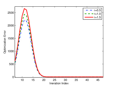
Figure 2: Comparison of convergence performance under different thresholds of the quantization scheme. Here the optimization error is defined as $\|x^{\ast}-x^{k}\|$.

VII-B Non-convex case

We use the decentralized training of a convolutional neural network (CNN) to evaluate the performance of our proposed decentralized stochastic optimization algorithm in non-convex optimization. More specially, we consider five agents interacting on a topology depicted in Fig. 1. The agents collaboratively train a CNN using the MNIST data set [64], which is a large benchmark database of handwritten digits widely used for training and testing in the field of machine learning [65]. Each agent has a local copy of the CNN. The CNN has 2 convolutional layers with 32 filters, and then two more convolutional layers with 64 filters each followed by a dense layer with 512 units. Each agent has access to a portion of the MNIST data set, which was further divided into two subsets for training and validation, respectively. We set the optimization parameters as $\lambda^{k}=\frac{1}{(0.001k+1)^{0.3}}$ and $\epsilon^{k}=\frac{1}{(0.001k+1)^{0.7}}$. For the adopted CNN model, the dimension of gradient, $d$, is equal to $1,676,266$. It can be verified that the parameters satisfy the conditions required in Theorem 1 and Corollary 1. The evolution of the training and validation accuracies averaged over 100 runs are illustrated by the solid and dashed black lines in Fig. 3. To compare the convergence performance of our algorithm with the conventional decentralized stochastic optimization algorithm, we also implemented the decentralized stochastic optimization algorithm in [20] to train the same CNN under the same quantization scheme, whose average training and validation accuracies over 100 runs are represented by the solid and dashed blue lines in Fig. 3. It can be seen that the proposed algorithm has a faster converging rate as well as better training/validation accuracy in the presence of quantization effects.

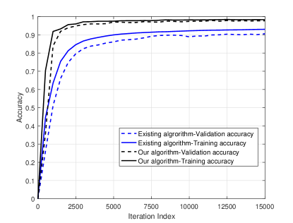
Figure 3: Comparison of CNN training/validation performance between our algorithm and the conventional decentralized stochastic optimization algorithm in [20].

To show that the proposed algorithm can indeed protect the privacy of participating agents, we also implemented a privacy attacker which tries to infer the raw image of participating agents using received information. The attacker implements the DLG attack model proposed in [26], which is the most powerful inference algorithm reported to date in terms of reconstructing exact raw data from shared gradients/model updates. The attacker was assumed to be able to eavesdrop all messages shared among the agents. Fig. 4 shows that the attacker could effectively recover the original training image from shared model updates in the conventional stochastic optimization algorithm in [20] that does not take privacy protection into consideration. However, under the proposed algorithm and quantization effects, the attacher failed to infer the original training image through information shared in the network. This is also corroborated by the attacker’s inference performance measured by the mean-square error (MSE) between the inference result and the original image. More specifically, as illustrated in Fig. 5, the attacker eventually inferred the raw image accurately as its estimation error converged to zero. However, the proposed approach successfully thwarted the attacker as attacker’s estimation error was always large.

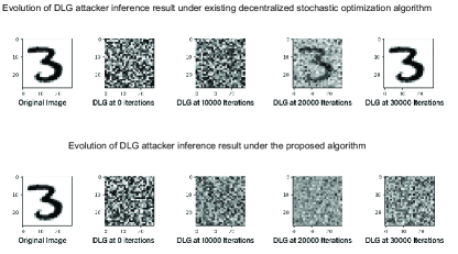
Figure 4: Comparison of DLG attacher’s inference results under existing decentralized stochastic optimization algorithm in [20] and our algorithm.

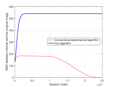
Figure 5: Comparison of DLG attacher’s inference errors under existing decentralized stochastic optimization algorithm in [20] and our algorithm.

VIII Conclusions

The paper has presented a decentralized stochastic optimization algorithm that is robust to aggressive quantization effects, which enables the exploitation of aggressive quantization effects to obfuscate shared information and hence enables privacy protection in decentralized stochastic optimization without losing provable convergence accuracy. Based on this result, this paper, for the first time, proposes and achieves ternary-quantization based rigorous ($0,\delta$)-differential privacy without losing provable convergence accuracy in decentralized stochastic optimization. The results are applicable in both the convex optimization case and the non-convex optimization case. The ternary quantization scheme also leads to significant reduction in communication overhead. Our approach appears to be the first to achieve rigorous differential privacy, communication efficiency, and provable convergence accuracy simultaneously in decentralized stochastic optimization. Both simulation results for a convex decentralized optimization problem and numerical experimental results for machine learning on a benchmark image dataset confirm the effectiveness of the proposed approach.

The paper assumes smooth gradients and does not consider potential constraints between optimization variables, as, for example, in [66]. In the future, we plan to extend the results to more general non-smooth and constrained decentralized optimization problems.

Appendix

VIII-A Some preliminary results

[67] Let $\{v^{k}\}$ be a non-negative sequence satisfying the following relationship for all $k\geq 0$:

$$v^{k+1}\leq(1+a^{k})v^{k}+w^{k}$$ (28)

where sequences $a^{k}\geq 0$ and $w^{k}\geq 0$ satisfy $\sum_{k=0}^{\infty}a^{k}<\infty$ and $\sum_{k=0}^{\infty}w^{k}<\infty$, respectively. Then the sequence $\{v^{k}\}$ will converge to a finite value $v\geq 0$.

[68, 23] Let $\{v^{k}\}$ be a non-negative sequence which satisfies the following relationship for all $k\geq 0$:

$$v^{k+1}\leq(1-r_{1}^{k})v^{k}+r_{2}^{k}$$ (29)

with sequences $r_{1}^{k}\geq 0$ and $r_{2}^{k}\geq 0$ satisfying

$$\frac{C_{1}}{(C_{3}k+1)^{\gamma_{1}}}\leq r_{1}^{k}\leq 1,\quad\frac{C_{2}}{(C_{3}k+1)^{\gamma_{2}}}\leq r_{2}^{k}\leq 1$$

for some $C_{1}>0$, $C_{2}>0$, $C_{3}>0$, $0\leq\gamma_{1}<1$, and $\gamma_{1}<\gamma_{2}$. Then $\lim_{k\rightarrow\infty}(k+1)^{\gamma_{0}}v^{k}=0$ holds for all $0\leq\gamma_{0}<\gamma_{2}-\gamma_{1}$.

Lemma 4.

[69] Suppose $h:\mathbb{R}^{d}\rightarrow\mathbb{R}$ is a convex function with gradient bounded by $G$. Then we have

$$|h(y)-h(x)|\leq G\|y-x\|$$

for any $x,y\in\mathbb{R}^{d}$

VIII-B Proof of Lemma 2

According to Lemma VIII-A in the Appendix, to prove that $\mathbb{E}\left[\|x^{k}\|^{2}\right]$ is bounded, we only need to prove that under the conditions in Lemma 2, it satisfies the inequality in (28) in the Appendix.

For the convenience of analysis, we first define the augmented versions of $x^{\ast}$ and $\bar{x}^{k}$:

$$\hat{x}^{\ast}\triangleq{\bf 1}_{m}\otimes x^{\ast},\quad\hat{\bar{x}}^{k}\triangleq{\bf 1}_{m}\otimes\bar{x}^{k}$$ (30)

where ${\bf 1}_{m}$ denotes an $m$ dimensional column vector with all entries equal to 1.

Using the inequality $(x+y)^{2}\leq 2x^{2}+2y^{2}$, which holds for any $x,y\in\mathbb{R}$, we can obtain

$$\|x^{k}\|^{2} =\|\hat{\bar{x}}^{k}-\hat{x}^{\ast}+x^{k}-\hat{\bar{x}}^{k}+\hat{x}^{\ast}\|^{2}$$ (31)

$$\leq(\|\hat{\bar{x}}^{k}-\hat{x}^{\ast}+x^{k}-\hat{\bar{x}}^{k}\|+\|\hat{x}^{\ast}\|)^{2}$$

$$\leq 2\|\hat{\bar{x}}^{k}-\hat{x}^{\ast}+x^{k}-\hat{\bar{x}}^{k}\|^{2}+2\|\hat{x}^{\ast}\|^{2}$$

$$\leq 2(\|\hat{\bar{x}}^{k}-\hat{x}^{\ast}\|+\|x^{k}-\hat{\bar{x}}^{k}\|)^{2}+2\|\hat{x}^{\ast}\|^{2}$$

$$\leq 4\|\hat{\bar{x}}^{k}-\hat{x}^{\ast}\|^{2}+4\|x^{k}-\hat{\bar{x}}^{k}\|^{2}+2\|\hat{x}^{\ast}\|^{2}$$

Because $\hat{x}^{\ast}$ is a constant, we will prove the boundedness of $\mathbb{E}\left[\|x^{k}\|^{2}\right]$ by proving that $\mathbb{E}\left[\|\hat{\bar{x}}^{k}-\hat{x}^{\ast}\|^{2}+\|x^{k}-\hat{\bar{x}}^{k}\|^{2}\right]$ is bounded. Our derivation will follow three steps: in Step I and Step II, we study the respective evolution of $\mathbb{E}\left[\|\hat{\bar{x}}^{k}-\hat{x}^{\ast}\|^{2}\right]$ and $\mathbb{E}\left[\|x^{k}-\hat{\bar{x}}^{k}\|^{2}\right]$ under our proposed algorithm in (3); in Step III, we show that $\mathbb{E}\left[\|\hat{\bar{x}}^{k}-\hat{x}^{\ast}\|^{2}+\|x^{k}-\hat{\bar{x}}^{k}\|^{2}\right]$ is bounded by combining the relationship obtained in Step I and Step II.

Step I: We first consider $\mathbb{E}\left[\|\hat{\bar{x}}^{k}-\hat{x}^{\ast}\|^{2}\right]$, which is equal to $m\mathbb{E}\left[\|{\bar{x}}^{k}-x^{\ast}\|^{2}\right]$ according to the definition in (30).

From (5), we have

$$\|\bar{x}^{k+1}-x^{\ast}\|^{2}= \left\|\bar{x}^{k}-x^{\ast}-\epsilon^{k}\lambda^{k}\frac{\sum_{i=1}^{m}g_{i}^{k}}{m}\right\|^{2}$$ (32)

$$\leq \left(\left\|\bar{x}^{k}-x^{\ast}\right\|+\left\|\epsilon^{k}\lambda^{k}\frac{\sum_{i=1}^{m}g_{i}^{k}}{m}\right\|\right)^{2}$$

Using the inequality $(x+y)^{2}\leq(1+\nu)x^{2}+(1+\frac{1}{\nu})y^{2}$, which holds for any $x,y\in\mathbb{R}$ and $\nu>0$, we can obtain the following relationship from (32) by setting $\nu$ to $(\epsilon^{k})^{2}$

$$\|\bar{x}^{k+1}-x^{\ast}\|^{2} \leq\left(1+(\epsilon^{k})^{2}\right)\left\|\bar{x}^{k}-x^{\ast}\right\|^{2}$$ (33)

$$\quad+\left(1+\frac{1}{(\epsilon^{k})^{2}}\right)\left\|\epsilon^{k}\lambda^{k}\frac{\sum_{i=1}^{m}g_{i}^{k}}{m}\right\|^{2}$$

$$=\left(1+(\epsilon^{k})^{2}\right)\left\|\bar{x}^{k}-x^{\ast}\right\|^{2}$$

$$\quad+\left((\epsilon^{k}\lambda^{k})^{2}+(\lambda^{k})^{2}\right)\left\|\frac{\sum_{i=1}^{m}g_{i}^{k}}{m}\right\|^{2}$$

$$\leq\left(1+(\epsilon^{k})^{2}\right)\left\|\bar{x}^{k}-x^{\ast}\right\|^{2}$$

$$\quad+\left((\epsilon^{k}\lambda^{k})^{2}+(\lambda^{k})^{2}\right)G^{2}$$

where we used the result that the gradient is bounded by $G$ from Lemma 1.

Step II: We next consider $\mathbb{E}\left[\|x^{k}-\hat{\bar{x}}^{k}\|^{2}\right]$. From (4) and (5), we can obtain the dynamics of $x^{k}-\hat{\bar{x}}^{k}$ based on the fact $A^{k}\bar{x}^{k}=\bar{x}^{k}$:

$$x^{k+1}-\hat{\bar{x}}^{k+1} =({A}^{k}\otimes I_{d})(x^{k}-\hat{\bar{x}}^{k})-\epsilon^{k}\lambda^{k}({M}\otimes I_{d})g^{k}$$ (34)

$$\quad+\epsilon^{k}(L_{w}\otimes I_{d})V^{k}$$

where $M=\left(I-\frac{{\bf 1}{\bf 1}^{T}}{m}\right)$ and the other parameters are given in (4). Therefore, we have

$$\|x^{k+1}-\hat{\bar{x}}^{k+1}\|^{2}$$ (35)

$$=\|(A^{k}\otimes I_{d})(x^{k}-\hat{\bar{x}}^{k})-\epsilon^{k}\lambda^{k}(M\otimes I_{d})g^{k}\|^{2}$$

$$\quad+\|\epsilon^{k}(L_{w}\otimes I_{d})V^{k}\|^{2}+$$

$$\quad 2\left\langle(A^{k}\otimes I_{d})(x^{k}-\hat{\bar{x}}^{k})-\epsilon^{k}\lambda^{k}(M\otimes I_{d})g^{k},\epsilon^{k}(L_{w}\otimes I_{d})V^{k}\right\rangle$$

i.e.,

$$\mathbb{E}\left[\|x^{k+1}-\hat{\bar{x}}^{k+1}\|^{2}\right]$$ (36)

$$=\mathbb{E}\left[\|(A^{k}\otimes I_{d})(x^{k}-\hat{\bar{x}}^{k})-\epsilon^{k}\lambda^{k}(M\otimes I_{d})g^{k}\|^{2}\right]$$

$$\quad+\mathbb{E}\left[\|\epsilon^{k}(L_{w}\otimes I_{d})V^{k}\|^{2}\right]$$

where we used the fact that $V^{k}$ is uncorrelated noise with expectation equal to zero.

It can be verified that the following relationship holds

$$\|(A^{k}\otimes I_{d}) (x^{k}-\hat{\bar{x}}^{k})-\epsilon^{k}\lambda^{k}(M\otimes I_{d})g^{k}\|$$

$$\leq\|(A^{k}\otimes I_{d})(x^{k}-\hat{\bar{x}}^{k})\|+\|\epsilon^{k}\lambda^{k}(M\otimes I_{d})g^{k}\|$$

$$\leq(1-\epsilon^{k}\rho)\|x^{k}-\hat{\bar{x}}^{k}\|+\|\epsilon^{k}\lambda^{k}(M\otimes I_{d})g^{k}\|$$

$$\leq(1-\epsilon^{k}\rho)\|x^{k}-\hat{\bar{x}}^{k}\|+\epsilon^{k}\lambda^{k}\|g^{k}\|$$

where the second inequality used the doubly-stochastic property of $A^{k}$ and Lemma 4.4 of [68] with $\rho$ the second largest eigenvalue of $L_{w}$, and the third inequality used the fact $\|M\|=1$. Therefore, we have

$$\| (A^{k}\otimes I_{d})(x^{k}-\hat{\bar{x}}^{k})-\epsilon^{k}\lambda^{k}(M\otimes I_{d})g^{k}\|^{2}$$

$$\leq(1+\nu)(1-\epsilon^{k}\rho)^{2}\|x^{k}-\hat{\bar{x}}^{k}\|^{2}+(1+\frac{1}{\nu})(\epsilon^{k}\lambda^{k})^{2}\|g^{k}\|^{2}$$

based on the inequality $(x+y)^{2}\leq(1+\nu)x^{2}+(1+\frac{1}{\nu})y^{2}$, which holds for any $x,y\in\mathbb{R}$ and $\nu>0$. Setting $\nu$ as $\epsilon^{k}\rho$, we further have

$$\|(A^{k}\otimes I_{d})(x^{k}-\hat{\bar{x}}^{k})-\epsilon^{k}\lambda^{k}(M\otimes I_{d})g^{k}\|^{2}$$ (37)

$$\leq(1+\epsilon^{k}\rho)(1-\epsilon^{k}\rho)^{2}\|x^{k}-\hat{\bar{x}}^{k}\|^{2}+(1+\frac{1}{\epsilon^{k}\rho})(\epsilon^{k}\lambda^{k})^{2}\|g^{k}\|^{2}$$

$$=(1-(\epsilon^{k})^{2}\rho^{2})(1-\epsilon^{k}\rho)\|x^{k}-\hat{\bar{x}}^{k}\|^{2}$$

$$\qquad+(1+\frac{1}{\epsilon^{k}\rho})(\epsilon^{k}\lambda^{k})^{2}\|g^{k}\|^{2}$$

$$\leq(1-\epsilon^{k}\rho)\|x^{k}-\hat{\bar{x}}^{k}\|^{2}+\left((\epsilon^{k}\lambda^{k})^{2}+\frac{\epsilon^{k}(\lambda^{k})^{2}}{\rho}\right)\|g^{k}\|^{2}$$

$$\leq(1-\epsilon^{k}\rho)\|x^{k}-\hat{\bar{x}}^{k}\|^{2}+\left((\epsilon^{k}\lambda^{k})^{2}+\frac{\epsilon^{k}(\lambda^{k})^{2}}{\rho}\right)G^{2}$$

Note that there always exists a $\beta>0$ such that $\mathbb{E}\left[\|V^{k}\|^{2}\right]<\beta\|x^{k}\|^{2}$ holds under Assumption 3, we can combine (36) and (37) to obtain

$$\mathbb{E}\left[\|x^{k+1}-\hat{\bar{x}}^{k+1}\|^{2}\right]\leq(1-\epsilon^{k}\rho)\mathbb{E}\left[\|x^{k}-\hat{\bar{x}}^{k}\|^{2}\right]$$ (38)

$$\qquad\qquad+\left((\epsilon^{k}\lambda^{k})^{2}+\frac{\epsilon^{k}(\lambda^{k})^{2}}{\rho}\right)G^{2}+(\epsilon^{k})^{2}\beta\mathbb{E}\left[\|x^{k}\|^{2}\right]$$

Step III: Finally, combining (31), (33), and (38) yields

$$\mathbb{E} \left[\|x^{k+1}-\hat{\bar{x}}^{k+1}\|^{2}+\|\bar{x}^{k+1}-x^{\ast}\|^{2}\right]$$ (39)

$$\leq(1-\epsilon^{k}\rho)\mathbb{E}\left[\|x^{k}-\hat{\bar{x}}^{k}\|^{2}\right]+\left((\epsilon^{k}\lambda^{k})^{2}+\frac{\epsilon^{k}(\lambda^{k})^{2}}{\rho}\right)G^{2}$$

$$\qquad+(\epsilon^{k})^{2}\beta\mathbb{E}\left[\|x^{k}\|^{2}\right]+(1+(\epsilon^{k})^{2})\mathbb{E}\left[\left\|\bar{x}^{k}-x^{\ast}\right\|^{2}\right]$$

$$\qquad+\left((\epsilon^{k}\lambda^{k})^{2}+(\lambda^{k})^{2}\right)G^{2}$$

$$\leq(1+(\epsilon^{k})^{2})\mathbb{E}\left[\|x^{k}-\hat{\bar{x}}^{k}\|^{2}+\left\|\bar{x}^{k}-x^{\ast}\right\|^{2}\right]$$

$$\qquad+(\epsilon^{k})^{2}\beta\mathbb{E}\left[\|x^{k}\|^{2}\right]$$

$$\qquad+\left(2(\epsilon^{k}\lambda^{k})^{2}+(1+\frac{\epsilon^{k}}{\rho})(\lambda^{k})^{2}\right)G^{2}$$

$$\leq(1+(\epsilon^{k})^{2}+4\beta(\epsilon^{k})^{2})\mathbb{E}\left[\|x^{k}-\hat{\bar{x}}^{k}\|^{2}+\left\|\bar{x}^{k}-x^{\ast}\right\|^{2}\right]$$

$$\qquad+\left(2(\epsilon^{k}\lambda^{k})^{2}+(1+\frac{\epsilon^{k}}{\rho})(\lambda^{k})^{2}\right)G^{2}+2\beta(\epsilon^{k})^{2})\|\hat{x}^{\ast}\|^{2}$$

Because the second and third terms on the right hand side of the above inequality are summable under the conditions in Lemma 2, according to Lemma VIII-A in the Appendix, we have that $\mathbb{E}\left[\|x^{k+1}-\hat{\bar{x}}^{k+1}\|^{2}+\|\bar{x}^{k+1}-x^{\ast}\|^{2}\right]$ will converge to a finite value. Further using (31) and the fact that $x^{\ast}$ is a finite vector, we have that $\mathbb{E}\left[\|x^{k}\|^{2}\right]$ is always bounded.

VIII-C Proof of Lemma 3

Noting that $\mathbb{E}\left[\|x^{k}\|^{2}\right]$ is bounded from Lemma 2, we always have the following inequality for some $\beta>0$ according to (38):

$$\mathbb{E}\left[\|x^{k+1}-\hat{\bar{x}}^{k+1}\|^{2}\right] \leq(1-\epsilon^{k}\rho)\mathbb{E}\left[\|x^{k}-\hat{\bar{x}}^{k}\|^{2}\right]$$ (40)

$$+\left((\epsilon^{k}\lambda^{k})^{2}+\frac{\epsilon^{k}(\lambda^{k})^{2}}{\rho}\right)G^{2}+(\epsilon^{k})^{2}\beta\Omega$$

where $\Omega$ is some constant representing an upper bound of $\mathbb{E}\left[\|x^{k}\|^{2}\right]$. Then the lemma can be directly obtained by applying Lemma VIII-A in Appendix A.

References

• [1] Nikolas Tsitsiklis. Problems in decentralized decision making and computation. Technical report, Massachusetts Inst of Tech Cambridge Lab for Information and Decision Systems, 1984.
• [2] Dimitri Bertsekas and John Tsitsiklis. Parallel and distributed computation: Numeral methods. 1989.
• [3] Socrates Deligeorges, George Cakiades, Jemin George, Yongqang Wang, and Francis Doyle. A mobile self synchronizing smart sensor array for detection and localization of impulsive threat sources. In 2015 IEEE International Conference on Multisensor Fusion and Integration for Intelligent Systems (MFI), pages 351–356. IEEE, 2015.
• [4] Chunlei Zhang and Yongqiang Wang. Distributed event localization via alternating direction method of multipliers. IEEE Transactions on Mobile Computing, 17(2):348–361, 2017.
• [5] Jorge Cortés, Sonia Martínez, and Francesco Bullo. Robust rendezvous for mobile autonomous agents via proximity graphs in arbitrary dimensions. IEEE Transactions on Automatic Control, 51(8):1289–1298, 2006.
• [6] Seyedbehzad Nabavi, Jianhua Zhang, and Aranya Chakrabortty. Distributed optimization algorithms for wide-area oscillation monitoring in power systems using interregional pmu-pdc architectures. IEEE Transactions on Smart Grid, 6(5):2529–2538, 2015.
• [7] Zhanhong Jiang, Aditya Balu, Chinmay Hegde, and Soumik Sarkar. Collaborative deep learning in fixed topology networks. In Proceedings of the 31st International Conference on Neural Information Processing Systems, pages 5906–5916, 2017.
• [8] Ran Xin, Soummya Kar, and Usman A Khan. Decentralized stochastic optimization and machine learning: A unified variance-reduction framework for robust performance and fast convergence. IEEE Signal Processing Magazine, 37(3):102–113, 2020.
• [9] Léon Bottou, Frank E Curtis, and Jorge Nocedal. Optimization methods for large-scale machine learning. SIAM Review, 60(2):223–311, 2018.
• [10] S Sundhar Ram, Angelia Nedić, and Venugopal V Veeravalli. Distributed stochastic subgradient projection algorithms for convex optimization. Journal of Optimization Theory and Applications, 147(3):516–545, 2010.
• [11] Angelia Nedić and Alex Olshevsky. Stochastic gradient-push for strongly convex functions on time-varying directed graphs. IEEE Transactions on Automatic Control, 61(12):3936–3947, 2016.
• [12] Dusan Jakovetic, Dragana Bajovic, Anit Kumar Sahu, and Soummya Kar. Convergence rates for distributed stochastic optimization over random networks. In 2018 IEEE Conference on Decision and Control (CDC), pages 4238–4245. IEEE, 2018.
• [13] Muhammed Sayin, Denizcan Vanli, Suleyman Kozat, and Tamer Başar. Stochastic subgradient algorithms for strongly convex optimization over distributed networks. IEEE Transactions on Network Science and Engineering, 4(4):248–260, 2017.
• [14] Shi Pu and Angelia Nedić. Distributed stochastic gradient tracking methods. Mathematical Programming, pages 1–49, 2020.
• [15] Michael Rabbat. Multi-agent mirror descent for decentralized stochastic optimization. In 2015 IEEE 6th International Workshop on Computational Advances in Multi-Sensor Adaptive Processing (CAMSAP), pages 517–520. IEEE, 2015.
• [16] Ohad Shamir and Nathan Srebro. Distributed stochastic optimization and learning. In 2014 52nd Annual Allerton Conference on Communication, Control, and Computing (Allerton), pages 850–857. IEEE, 2014.
• [17] Benjamin Sirb and Xiaojing Ye. Decentralized consensus algorithm with delayed and stochastic gradients. SIAM Journal on Optimization, 28(2):1232–1254, 2018.
• [18] Pascal Bianchi and Jérémie Jakubowicz. Convergence of a multi-agent projected stochastic gradient algorithm for non-convex optimization. IEEE Transactions on Automatic Control, 58(2):391–405, 2012.
• [19] Tatiana Tatarenko and Behrouz Touri. Non-convex distributed optimization. IEEE Transactions on Automatic Control, 62(8):3744–3757, 2017.
• [20] Xiangru Lian, Ce Zhang, Huan Zhang, Cho-Jui Hsieh, Wei Zhang, and Ji Liu. Can decentralized algorithms outperform centralized algorithms? a case study for decentralized parallel stochastic gradient descent. In Advances in Neural Information Processing Systems, 2017.
• [21] Navjot Singh, Deepesh Data, Jemin George, and Suhas Diggavi. Sparq-sgd: Event-triggered and compressed communication in decentralized optimization. In 2020 59th IEEE Conference on Decision and Control (CDC), pages 3449–3456. IEEE, 2020.
• [22] Anastasia Koloskova, Sebastian Stich, and Martin Jaggi. Decentralized stochastic optimization and gossip algorithms with compressed communication. In International Conference on Machine Learning, pages 3478–3487. PMLR, 2019.
• [23] Jemin George, Tao Yang, He Bai, and Prudhvi Gurram. Distributed stochastic gradient method for non-convex problems with applications in supervised learning. In Proceedings of the IEEE 58th Conference on Decision and Control (CDC), pages 5538–5543. IEEE, 2019.
• [24] C. Zhang, M. Ahmad, and Y. Q. Wang. ADMM based privacy-preserving decentralized optimization. IEEE Transactions on Information Forensics and Security, 14(3):565–580, 2019.
• [25] Luca Melis, Congzheng Song, Emiliano De Cristofaro, and Vitaly Shmatikov. Exploiting unintended feature leakage in collaborative learning. In 2019 IEEE Symposium on Security and Privacy (SP), pages 691–706. IEEE, 2019.
• [26] Ligeng Zhu, Zhijian Liu, and Song Han. Deep leakage from gradients. In Advances in Neural Information Processing Systems, pages 14774–14784, 2019.
• [27] Pascal Paillier. Public-key cryptosystems based on composite degree residuosity classes. In International Conference on the Theory and Applications of Cryptographic Techniques, pages 223–238. Springer, 1999.
• [28] Andrew Chi-Chih Yao. How to generate and exchange secrets. In 27th Annual Symposium on Foundations of Computer Science, pages 162–167. IEEE, 1986.
• [29] Nick Hynes, Raymond Cheng, and Dawn Song. Efficient deep learning on multi-source private data. arXiv preprint arXiv:1807.06689, 2018.
• [30] Chunlei Zhang and Yongqiang Wang. Enabling privacy-preservation in decentralized optimization. IEEE Transactions on Control of Network Systems, 6(2):679–689, 2018.
• [31] Yasser Shoukry, Konstantinos Gatsis, Amr Alanwar, George J Pappas, Sanjit A Seshia, Mani Srivastava, and Paulo Tabuada. Privacy-aware quadratic optimization using partially homomorphic encryption. In 2016 IEEE 55th Conference on Decision and Control (CDC), pages 5053–5058. IEEE, 2016.
• [32] Yang Lu and Minghui Zhu. Privacy preserving distributed optimization using homomorphic encryption. Automatica, 96:314–325, 2018.
• [33] Andreea B Alexandru, Konstantinos Gatsis, Yasser Shoukry, Sanjit A Seshia, Paulo Tabuada, and George J Pappas. Cloud-based quadratic optimization with partially homomorphic encryption. IEEE Transactions on Automatic Control, 2020.
• [34] Raef Bassily, Adam Smith, and Abhradeep Thakurta. Private empirical risk minimization: Efficient algorithms and tight error bounds. In Proceedings of IEEE 55th Annual Symposium on Foundations of Computer Science, pages 464–473. IEEE, 2014.
• [35] Zhenqi Huang, Sayan Mitra, and Nitin Vaidya. Differentially private distributed optimization. In Proceedings of the 2015 International Conference on Distributed Computing and Networking, pages 1–10, 2015.
• [36] Jorge Cortés, Geir E Dullerud, Shuo Han, Jerome Le Ny, Sayan Mitra, and George J Pappas. Differential privacy in control and network systems. In 2016 IEEE 55th Conference on Decision and Control (CDC), pages 4252–4272. IEEE, 2016.
• [37] Xueru Zhang, Mohammad Mahdi Khalili, and Mingyan Liu. Recycled ADMM: Improving the privacy and accuracy of distributed algorithms. IEEE Transactions on Information Forensics and Security, 15:1723–1734, 2019.
• [38] Cynthia Dwork, Aaron Roth, et al. The algorithmic foundations of differential privacy. Foundations and Trends in Theoretical Computer Science, 9(3-4):211–407, 2014.
• [39] Qiongxiu Li, Richard Heusdens, and Mads Græsbøll Christensen. Privacy-preserving distributed optimization via subspace perturbation: a general framework. IEEE Transactions on Signal Processing, 68:5983–5996, 2020.
• [40] Feng Yan, Shreyas Sundaram, SVN Vishwanathan, and Yuan Qi. Distributed autonomous online learning: Regrets and intrinsic privacy-preserving properties. IEEE Transactions on Knowledge and Data Engineering, 25(11):2483–2493, 2012.
• [41] Youcheng Lou, Lean Yu, Shouyang Wang, and Peng Yi. Privacy preservation in distributed subgradient optimization algorithms. IEEE Transactions on Cybernetics, 48(7):2154–2165, 2017.
• [42] Shripad Gade and Nitin H Vaidya. Privacy-preserving distributed learning via obfuscated stochastic gradients. In 2018 IEEE Conference on Decision and Control (CDC), pages 184–191. IEEE, 2018.
• [43] Yongqiang Wang and H Vincent Poor. Decentralized stochastic optimization with inherent privacy protection. IEEE Transactions on Automatic Control, 2022.
• [44] Yongqiang Wang and Angelia Nedić. Decentralized gradient methods with time-varying uncoordinated stepsizes: Convergence analysis and privacy design. arXiv preprint arXiv:2205.10934, 2022.
• [45] A Reisizadeh, H Taheri, A Mokhtari, H Hassani, and R Pedarsani. Robust and communication-efficient collaborative learning. Advances in Neural Information Processing Systems 32 (NIPS 2019), 2019.
• [46] Albert S Berahas, Charikleia Iakovidou, and Ermin Wei. Nested distributed gradient methods with adaptive quantized communication. In 2019 IEEE 58th Conference on Decision and Control (CDC), pages 1519–1525. IEEE, 2019.
• [47] Amirhossein Reisizadeh, Aryan Mokhtari, Hamed Hassani, and Ramtin Pedarsani. An exact quantized decentralized gradient descent algorithm. IEEE Transactions on Signal Processing, 67(19):4934–4947, 2019.
• [48] Oded Goldreich. Foundations of Cryptography: volume 2, Basic Applications. Cambridge University Press, 2001.
• [49] Yongqiang Wang. Privacy-preserving average consensus via state decomposition. IEEE Transactions on Automatic Control, 64(11):4711–4716, 2019.
• [50] Minghao Ruan, Huan Gao, and Yongqiang Wang. Secure and privacy-preserving consensus. IEEE Transactions on Automatic Control, 64(10):4035–4049, 2019.
• [51] Sebastian Meiser. Approximate and probabilistic differential privacy definitions. IACR Cryptol. ePrint Arch., 2018:277, 2018.
• [52] Angelia Nedic. Distributed gradient methods for convex machine learning problems in networks: Distributed optimization. IEEE Signal Processing Magazine, 37(3):92–101, 2020.
• [53] Bahman Gharesifard and Jorge Cortés. Distributed strategies for generating weight-balanced and doubly stochastic digraphs. European Journal of Control, 18(6):539–557, 2012.
• [54] Michael G Rabbat and Robert D Nowak. Quantized incremental algorithms for distributed optimization. IEEE Journal on Selected Areas in Communications, 23(4):798–808, 2005.
• [55] Peng Yi and Yiguang Hong. Quantized subgradient algorithm and data-rate analysis for distributed optimization. IEEE Transactions on Control of Network Systems, 1(4):380–392, 2014.
• [56] Ye Pu, Melanie N Zeilinger, and Colin N Jones. Quantization design for distributed optimization. IEEE Transactions on Automatic Control, 62(5):2107–2120, 2016.
• [57] Jiaqi Zhang, Keyou You, and Tamer Başar. Distributed discrete-time optimization in multiagent networks using only sign of relative state. IEEE Transactions on Automatic Control, 64(6):2352–2367, 2019.
• [58] Xuanyu Cao and Tamer Başar. Decentralized online convex optimization based on signs of relative states. Automatica, 129:109676, 2021.
• [59] Hassan K Khalil. Nonlinear systems. Prentice hall Upper Saddle River, NJ, 2002.
• [60] Dan Alistarh, Demjan Grubic, Jerry Z Li, Ryota Tomioka, and Milan Vojnovic. QSGD: communication-efficient sgd via gradient quantization and encoding. In Proceedings of the 31st International Conference on Neural Information Processing Systems, pages 1707–1718, 2017.
• [61] Wei Wen, Cong Xu, Feng Yan, Chunpeng Wu, Yandan Wang, Yiran Chen, and Hai Li. Terngrad: ternary gradients to reduce communication in distributed deep learning. In Proceedings of the 31st International Conference on Neural Information Processing Systems, pages 1508–1518, 2017.
• [62] Peter Kairouz, Sewoong Oh, and Pramod Viswanath. The composition theorem for differential privacy. In International Conference on Machine Learning, pages 1376–1385. PMLR, 2015.
• [63] Naman Agarwal, Ananda Theertha Suresh, Felix Xinnan X Yu, Sanjiv Kumar, and Brendan McMahan. cpSGD: Communication-efficient and differentially-private distributed SGD. Advances in Neural Information Processing Systems, 31, 2018.
• [64] Yann LeCun, Corinna Cortes, Christopher, and J. C. Burges. The MNIST database of handwritten digits. http://yann.lecun.com/exdb/mnist/, 1994.
• [65] Li Deng. The MNIST database of handwritten digit images for machine learning research [best of the web]. IEEE Signal Processing Magazine, 29(6):141–142, 2012.
• [66] Xuanyu Cao and Tamer Başar. Decentralized multi-agent stochastic optimization with pairwise constraints and quantized communications. IEEE Transactions on Signal Processing, 68:3296–3311, 2020.
• [67] Herbert Robbins and David Siegmund. A convergence theorem for non negative almost supermartingales and some applications. In Optimizing methods in statistics, pages 233–257. Elsevier, 1971.
• [68] Soummya Kar, José MF Moura, and H Vincent Poor. Distributed linear parameter estimation: Asymptotically efficient adaptive strategies. SIAM Journal on Control and Optimization, 51(3):2200–2229, 2013.
• [69] Angelia Nedić, Alex Olshevsky, and Michael G Rabbat. Network topology and communication-computation tradeoffs in decentralized optimization. Proceedings of the IEEE, 106(5):953–976, 2018.