Robust Machine Learning for Malware Detection over Time

Abstract

The presence and persistence of Android malware is an on-going threat that plagues this information era, and machine learning technologies are now extensively used to deploy more effective detectors that can block the majority of these malicious programs. However, these algorithms have not been developed to pursue the natural evolution of malware, and their performances significantly degrade over time because of such concept-drift.

Currently, state-of-the-art techniques only focus on detecting the presence of such drift, or they address it by relying on frequent updates of models. Hence, there is a lack of knowledge regarding the cause of the concept drift, and ad-hoc solutions that can counter the passing of time are still under-investigated.

In this work, we commence to address these issues as we propose (i) a drift-analysis framework to identify which characteristics of data are causing the drift, and (ii) SVM-CB, a time-aware classifier that leverages the drift-analysis information to slow down the performance drop. We highlight the efficacy of our contribution by comparing its degradation over time with a state-of-the-art classifier, and we show that SVM-CB better withstands the distribution changes that naturally characterize the malware domain. We conclude by discussing the limitations of our approach and how our contribution can be taken as a first step towards more time-resistant classifiers that not only tackle, but also understand the concept drift that affects data.

0.1 Introduction

In this information era, we are experiencing tremendous growth in mobile technology, both in its efficacy and pervasiveness. One of the most common operating systems for mobile devices is Android,  and, because of its popularity, it became particularly attractive to cyber-attackers eyes, who exploit Android vulnerabilities creating malicious applications, also known as malware, targeted specifically for these systems . Luckily, the technological development of this era brings enough power to machine learning algorithms, considered the standard for many domains, including cyber-security and, specifically, malware detection, which has shown to be very effective also against never-seen malware families [1, 2, 3, 4, 5, 6].

However, real-world data experience a phenomenon known as concept drift, i.e. their temporal evolution [7]. In particular, Android applications naturally change over time since attackers keep adjusting malware to bypass detection, and legitimate applications embrace new frameworks and programming patterns while abandoning deprecated technologies. Recent work highlighted how concept drift worryingly affects the performance of state-of-the-art Android malware detectors, revealing how much it drops over time, contradicting the results achieved by their original analysis since they were inflated by wrong evaluation settings [8]. On top of this issue, the only proposals to counter the concept drift rely on continuous update or retraining of machine learning models [9, 10, 11, 12, 13], instead of tracking which are the characteristics of data that mainly change over time.

Hence, we start bridging the gaps left in the state-of-the-art by proposing novel techniques that understand the concept drift and take advantage of it. The contribution of this work are summarized as follows: (i) we propose a drift-analysis framework that investigates the reasons causing the concept drift inside data, highlighting which features are more prone to have a negative contribution to the performance decay; and (ii) we propose SVM-CB, a novel classifier that leverages our drift-analysis information to bound the selected unstable features, reducing the overall performance drop.

We show the effectiveness of SVM-CB, by comparing its performance over time with Drebin [1], a state-of-the-art linear classifier. To obtain a fair comparison, we train both classifiers on the same dataset, and we show how SVM-CB better withstand the passing of time, thanks to the domain knowledge acquired through the results of our drift-analysis framework, thus allowing SVM-CB to be updated less often compared to Drebin.

We conclude by discussing future directions of this work considering fewer heuristic rules to tune SVM-CB, and extensions of our methodology to non-linear classifiers.

0.2 Android Malware Detection over Time

Before delving into the details of the proposed methods, we firstly describe the structure of Android applications to lay a foundation for understanding the classifier that we consider in this work, and we discuss the problem and proposed solutions to the concept drift problem.

Android Applications. These are programs that run on the Android Operating System. They are distributed as an Android Application Package (APK), an archive file with the .apk extension. An APK contains different files: (i) the AndroidManifest.xml, that stores all the required information needed by the operating system to correctly handle the application at run-time; (ii) the classes.dex, that stores the compiled source code and all user-implemented methods and classes; and (iii) additional .xml and resource files that are used to define the application user interface, along with additional functionality or multimedia content.

Malware Detection with Machine Learning. We select a popular binary detector named Drebin [1] as a baseline for our proposals, for which we show the architecture in Fig .whose architecture is described in Fig. 1. This classifier relies on a Support Vector Machine (SVM) [14] trained on top of hand-crafted features extracted from APKs provided at training time, and they consider: (i) features extracted from AndroidManifest.xml, like hardware components, requested permissions, app components, and filtered intents; (ii) features extracted from classess.dex, including restricted API calls, used permissions, suspicious API calls, and network addresses. All this knowledge is encoded inside $d$-dimensional feature vectors, whose entries are 0 or 1 depending on the absence or presence of a particular characteristic. Since Drebin relies on an SVM, it can be used to investigate its decision-making process since each feature is already correlated with a weight that describes its orientation toward one of the two prediction classes, namely legit and malicious.

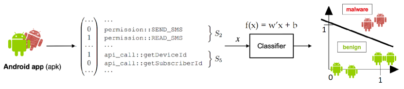
Figure 1: A schematic representation of Drebin [1]. First, applications are represented as binary vectors in a $d$-dimensional feature space, and this corpus of data is used to train an SVM. At test time, unseen applications are fed into a linear classifier, and they are classified as malware if their score $f(x)\geq 0$.

Performance over Time. Even though Drebin registered impressive performance in detecting malware, it was not properly tested inside a time-aware environment. I ts training relies on the Independent and Identical Distribution (I.I.D.) assumption, which takes for granted that both training and testing samples are drawn from the same distribution. While this property might hold for the image classification domain, it can not be satisfied for the rapidly-growing domain of programs, where training samples differ from future test data as new updates, frameworks, and techniques are introduced while others are deprecated. The classic evaluation setting injects artifacts inside the learning process, like the presence of samples coming from mixed periods, allowing the classifier to rely on future knowledge at training time. Such has been demonstrated by Pendlebury et al. [8], that show how selected state-of-the-art detectors are characterized by worrying performance drops when evaluated with a more realistic time-aware approach.

0.3 Analysing and Improving Robustness to Time

We now introduce the two contributions of our work: (i) the drift-analysis framework to either understand the causes of the concept drift by inspecting the features extracted from data at different time intervals and quantifying their contribution to the overall performance drop; and (ii) the time-aware learning algorithm SVM-CB (i.e. SVM with Custom Bounds), that uses drift-analysis information to select and bound the weights of a chosen number of features considered unstable to reduce their contribution to the performance decay caused by time.

Drift-analysis framework. Our first contribution tackles the open problem of explaining the concept drift, and we propose the temporal feature stability (T-stability), a novel metric measuring the single feature contribution to the performance decay, designed for linear classifiers. This metric captures two distinct characteristics of each single feature when dealing with time: their relevance in the classifier prediction and their temporal evolution. These are quantified by the product between (i) the weight $w_{j}$ corresponding to the $j$-th feature, learned at training time by the classifier; and (ii) the slope $m_{j}$ that approximates the temporal evolution of the values of the feature.

To compute our metric, we start with the hypothesis that a decrement in the detection rate of malware is strictly related to a decaying score assigned to malware samples as time passes. Such behavior corresponds to a shift of the malware class distribution towards the decision boundary learned at training time, thus increasing the number of misclassified samples. To quantify our intuitions, we analyze the variation of the malware score over time, and we compute the conditional expectation of the score over all malware samples (identified with the label $y=1$) at time $t$ as:

$$E[\boldsymbol{w}^{T}\boldsymbol{x}+b|y=1,t]=E\left[\left(\sum_{j=0}^{d}w_{j}\cdot x_{i,j}\right)+b|y=1,t\right]=\left[\sum_{j=0}^{d}w_{j}\cdot E[x_{i,j}|y=1,t]\right]+b$$ (1)

where the score is computed as the scalar product between $\boldsymbol{w}$, the vector containing the weights of the linear classifier with bias $b$, and $\boldsymbol{x}_{i}$ the $d$-dimensional feature vector representation of an input Android application.

Since we want to quantify how the features contribute to the score expectation evolution, we consider the derivative of Eq. 1, being the summation over the products between weights and the derivatives of the feature expectation w.r.t. time.

$$\frac{dE[\boldsymbol{w}^{T}\boldsymbol{x}+b|y,t]}{dt}=\sum_{j=1}^{d-1}w_{j}\cdot\frac{dE[x_{j}|y,t]}{dt}\approx\sum_{j=0}^{d-1}w_{j}\cdot m_{j}=\sum_{j=1}^{d-1}\delta_{j}$$ (2)

Since we are interested in capturing the overall trend of the score decay, we approximate each derivative of the $j$-th feature with the slope $m_{j}$ of the regression line that best fits the single feature expectation over time. Here, we compress the product $w_{j}\cdot m_{j}$ in a single value $\delta_{j}$, that is how we compute the T-stability of the feature $j$. Intuitively, the larger and negative the T-stability metric is for a feature, the more such feature accelerates the degradation of the classifier.

Since expectations are not computable for a specific time instant $t$, we quantize the time variable considering time slots with length $\Delta t$, where the $k$-th slot indicate the subset $D_{k}$ of malware samples registered at time $t\in[k\Delta t,(k+1)\Delta t]$, being $k$ an integer variable. Thus, we use Alg. 1 to obtain the vector $\boldsymbol{\delta}$ containing the T-stability of each feature. After having computed the number of available time slots $T$ based on the timestamps in $\mathcal{D}$, and the chosen time window $\Delta t$ (line 1), we initialize a utility matrix $M_{dxT}$ that will contain the mean feature values (line 1). Then we iterate through the time slots (line 1) and select, for each one, the subset $D_{k}$ (line 1) needed to compute the mean feature value at time $k\Delta t$ storing it in the $k$-th column of $M$ (line 1). After this step, we loop over the number of features (line 1) to compute the slope $m_{j}$ of the $j$-th feature over time, i.e. the $j$-th row of $M$ (line 1), to eventually return the Hadamard product between the classifier trained weights $\boldsymbol{w}$ and the feature slopes $\boldsymbol{m}$ (line 1), i.e. the T-stability vector $\boldsymbol{\delta}$.

Input : The input timestamped and labeled dataset $\mathcal{D}=\{\boldsymbol{x}_{i},y_{i},t_{i}\}_{i=1}^{n}$; the time window $\Delta t$; the weights $\boldsymbol{w}$ of the reference classifier $g^{\prime}$.

Output : the T-stability vector $\boldsymbol{\delta}$

1

$T\leftarrow\lceil(t_{max}-t_{min})/\Delta t\rceil$

  $\triangleright$ Compute number of time slots

2

$M\leftarrow zeros(d,T)$

  $\triangleright$ Initialize utility matrix

3

4for $k\in[0,T-1]$ do

       $\mathcal{D}_{k}\leftarrow\{(\boldsymbol{x}_{i},y_{i},t_{i})\in\mathcal{D}:y_{i}=1,t_{i}\in[k\Delta t,(k+1)\Delta t]\}$

        $\triangleright$ Obtain data in time slot $k$

5      

      $M_{*,k}\leftarrow\frac{1}{|D_{k}|}\sum_{x_{i}\in D_{k}}x_{i,*}$

        $\triangleright$ Compute mean feature value in time slot $k$

6      

7

8$\boldsymbol{m}\leftarrow zeros(d)$

9for $j\in[0,d-1]$ do

       $m_{j}\leftarrow fit(M_{j,*})$

        $\triangleright$ Compute slope of the regression line

10      

11

$\boldsymbol{\delta}\leftarrow\boldsymbol{w}\circ\boldsymbol{m}$

  $\triangleright$ Compute the T-stability vector

12

return $\boldsymbol{\delta}$

  $\triangleright$ Return T-stability vector

Algorithm 1 Drift Analysis

Robustness to Future Changes. As our second contribution, we show how to exploit the information obtained with the drift-analysis inside the optimization process to train SVM-CB, an SVM classifier hardened against the passing of time. To train SVM-CB, we consider a reference temporally unstable classifier to compute the T-stability for each feature. Then, we select the unstable features, that are the $n_{f}$ of them that have the most negative $\delta_{j}$ values. Our goal is to train a new classifier that relies less on these unstable features, thus we bound the absolute value of the correspondent weights to directly reduce their contribution in Eq. 2. This can be formalized as the constrained optimization problem in Eq. 3, where the hinge loss is minimized subject to a constrained on the subset of weights $\mathcal{W}_{f}$, i.e. the $n_{f}$ weights correspondent to the unstable features, that are forced to be lower than a specific bound ${r}$ in their absolute value.

$$\operatornamewithlimits{\arg\,\min}_{\boldsymbol{w},b} \sum_{i=1}^{n}max(0,1-y_{i}f(\boldsymbol{x}_{i};\boldsymbol{w},b)),$$ (3)

$$s.t. |w_{j}|<{r},\forall w_{j}\in\mathcal{W}_{f}.$$ (4)

We show in Alg. 2 the time-aware training algorithm for SVM-CB that minimize this objective through a gradient descent procedure. The algorithm is initialized by firstly identifying the subset $\mathcal{W}_{f}$ of weights corresponding to the $n_{f}$ unstable features (lines 2-2). Then, for each iteration, we firstly modulate the learning rate with the function $s(t)$ to improve convergence (line  2), we update the parameters of the classifier to train by applying gradient descent (lines 2-2), to eventually clip the weights contained in $\mathcal{W}_{f}$ to the bound ${r}$ if their absolute value exceed it (line 2), as described in Eq. 4. After $N$ iterations, the algorithm returns the learned parameters $\boldsymbol{w}$ and $b$.

Input : $\mathcal{D}=\{\boldsymbol{x}_{i},\boldsymbol{y}_{i}\}_{i=1}^{n}$, the training data; ${r}$, the absolute value of the bound that must be applied to the weights; $\delta$, the T-stability vector; $n_{f}$, the number of weights that must be bounded; $N$, the number of iterations; $\eta^{(0)}$, the initial gradient step size ; $s(t)$ a decaying function of $t$.

Output : $\boldsymbol{w},b$, the trained classifier’s parameters.

1

$\mathcal{J}\leftarrow argsort(\boldsymbol{\delta})$

  $\triangleright$ Initialize feature indexes ordered w.r.t. $\delta$

2

$\mathcal{J}_{f}\leftarrow\{j_{k}:k=0,...,n_{f}\},j_{k}\in\mathcal{J}.$

  $\triangleright$ Select first $n_{f}$ indexes

Initialize $\mathcal{W}_{f}=\{w_{j}:j\in\mathcal{J}_{f}\}$

  $\triangleright$ Select corresponding $n_{f}$ weights

3

$(\boldsymbol{w}^{(0)},b^{(0)})\leftarrow(\boldsymbol{0},0)$

  $\triangleright$ Initialize parameters

4

5for $t\in[1,N]$ do

       $\eta^{(t)}\leftarrow\eta^{(0)}s(t)$

        $\triangleright$ Update learning rate

6      

      $\boldsymbol{w}^{(t)}\leftarrow\boldsymbol{w}^{(t-1)}-\eta^{(t)}\nabla_{\boldsymbol{w}}\mathcal{L}$

        $\triangleright$ Update weights

7      

      $b^{(t)}\leftarrow b^{(t-1)}-\eta^{(t)}\nabla_{b}\mathcal{L}$

        $\triangleright$ Update bias

8      

      $\boldsymbol{w}^{(t)}\leftarrow Clip(\boldsymbol{w}^{(t)};\mathcal{W}_{f},{r})$

        $\triangleright$ Clip weights based on Eq. 4 criteria

9      

10

return $\boldsymbol{w}^{(t)},b^{(t)}$

  $\triangleright$ Return the learned parameters

11

Algorithm 2 SVM-CB learning algorithm

0.4 Experiments

We now apply our methodology to quantify how it explains and hardens a classifier against the performance decay compared with the time-agnostic classifier Drebin [1].

Dataset. We leverage the dataset provided by Pendlebury et al. [8], composed of 116,993 legitimate and 12,735 malicious Android applications sampled from the AndroZoo dataset [15], spanning from January 2014 to December 2016. We replicate their temporal train-test split as shown in Fig. 2, by dividing them between December 2014 and January 2015, and we set the time slot $\Delta t$ equal to $1$ month to ensure sufficient statistics for each. We hence extract 465,608 from the training set to match the original formulation of Drebin [1].

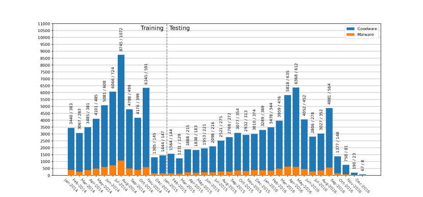
Figure 2: Stack histogram with the monthly distribution of apps, spanning from Jan 2014 to Dec 2016. The dashed vertical lines determine the considered time-aware temporal split.

Models. We consider Drebin as the baseline classifier, trained with the $C$ parameter set to $1$, and we compare it with two versions of SVM-CB by considering different bounds on the unstable features detected by the drift-analysis framework. We will refer to the baseline classifier as SVM since the underlying feature extractor and the feature embedding module are the same for all the classifiers under analysis.

Drift Analysis Results. To identify the features responsible for the performance decay over time in our baseline SVM, we firstly show in Fig. 3 the trend of the mean score assigned respectively to malicious (Fig. 3(a)) and benign samples (Fig. 3(b)) over all the testing periods. While the classifier assigns, on average, an almost constant negative score to the goodware class, the mean score assigned to malware gradually approaches to zero to eventually become negative after 10 months, thus validating the hypothesis claimed in Sect. 0.3.

We compute the T-stability vector $\boldsymbol{\delta}$ through Alg. 1 for the learned weights of the SVM w.r.t. the timestamped training set, and we show the first $10^{4}$ T-stability values in increasing order along with the corresponding features in Fig. 3(c). The latter highlights that most of the contribution to the performance decay is caused by roughly 100 features among all the feature set, while all the remaining ones do not substantially compromise the detection rate over time since their T-stability is very close to zero.

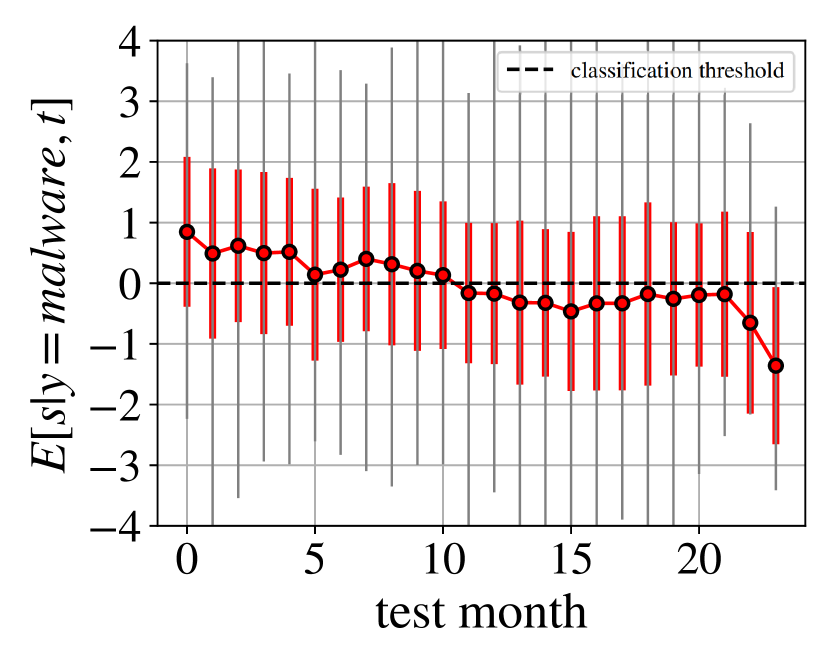
(a)

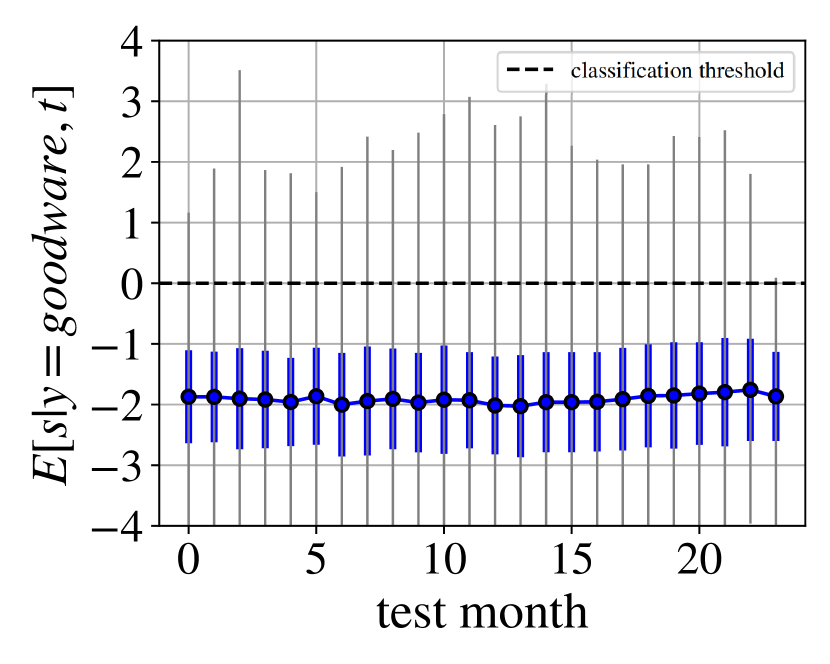
(b)

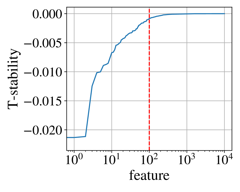
(c)

Figure 3: The mean score over the testing periods assigned by the SVM to malware (a) and goodware samples (b) of the test set, along with their standard deviation (colored thick lines) and min-max range(thin grey lines). Lastly, the $10^{4}$ T-stability values in increasing order, computed through Alg. 1 (c).

We report a subset of the selected unstable features (i.e. features presenting large negative T-stability values) in Table 1. The first 10 rows show features that the SVM associates with the goodware class and are becoming more likely to be found in malware ($w_{j}<0,m_{j}>0$), while the last 10 rows show features that the SVM associates with the malware class but they are disappearing from data ($w_{j}>0$, $m_{j}<0$). For simplicity, we will refer to the features in the first and second table, respectively, as the first and the second group of features.

We can recognize in the first group features mostly related to commonly-used URLs. For instance, among them, we find “www.google.com”, “www.youtube.com”, and websites under the “facebook.com” domain, which are all legitimate URLs to browse, and the classifier links them to the goodware class by assigning them a positive weight. The second group is mostly characterized by features related to intents and activities. For instance, we find the presence of a cipher algorithm (“interesting_calls::Cipher(DES)”), reported to be used to obfuscate and encrypt part of the malicious application. However, this feature has a decreasing trend ($m_{j}<0$), meaning that malware relies less on this method as time passes, probably because it would ease the detection of the malware under manual inspection.

From this analysis, we can deduce that the unstable features can be grouped into two types of features: (i) goodware-related features that malware creators are starting to inject in their malicious code to increase the probability of it being recognized as goodware, and (ii) malware-related features that malware creators are starting to deprecate to reduce the probability of it being recognized as malware.

Table 1: List of 20 features taken from the set of unstable features. The first column contains the considered features, the second column represents their T-stability measure $\delta_{j}$, the third column the weight $w_{j}$ assigned by the SVM, and the fourth column is the estimated angular coefficient $m_{j}$. The first 10 rows show goodware-related features which are becoming more frequent in malware as time passes, while the last 10 rows show malware-related features which are disappearing from this class.

Feature name	$\delta_{j}$	$w_{j}$	$m_{j}$
urls::https://graph.facebook.com/%1$s?…&accessToken=%2$s	-0.008753	-0.596730	0.014669
intents::android_intent_action_VIEW	-0.010168	-0.462059	0.022005
urls::http://www.google.com	-0.021320	-0.436577	0.048835
activities::com_revmob_ads_fullscreen_FullscreenActivity	-0.006204	-0.348884	0.017782
activities::com_feiwo_view_IA	-0.004435	-0.347665	0.012758
urls::http://i.ytimg.com/vi/	-0.005245	-0.319063	0.016438
api_calls::android/content/ContentResolver;$\rightarrow$openInputStream	-0.003749	-0.302131	0.012410
urls::https://m.facebook.com/dialog/	-0.004955	-0.285100	0.017379
urls::http://market.android.com/details?id=	-0.004041	-0.260522	0.015510
urls::http://www.youtube.com/embed/	-0.004289	-0.259927	0.016502
api_calls::android/net/wifi/WifiManager;$\rightarrow$getConnectionInfo	-0.003469	0.148022	-0.023438
app_permissions::name=’android_permission_MOUNT_UNMOUNT_FILESYSTEMS’	-0.004508	0.296193	-0.015220
urls::http://e.admob.com/clk?…	-0.006713	0.427714	-0.015695
activities::com_feiwothree_coverscreen_SA	-0.003564	0.443662	-0.008034
interesting_calls::Cipher(DES)	-0.008910	0.489497	-0.018202
intents::android_intent_action_PACKAGE_ADDED	-0.022435	0.702801	-0.031922
activities::com_fivefeiwo_coverscreen_SA	-0.003813	0.743198	-0.005131
intents::android_intent_action_CREATE_SHORTCUT	-0.012456	0.748091	-0.016650
intents::android_intent_action_USER_PRESENT	-0.021155	0.803000	-0.026344
activities::com_feiwoone_coverscreen_SA	-0.010022	1.141652	-0.008778

Improving Robustness. We now leverage the results of our drift-analysis framework performed on the SVM by training SVM-CB using Alg. 2, running it for 2000 iterations, with the initial learning rate $\eta^{(0)}$ set to $7\cdot 10^{-5}$ and we use the cosine annealing function as $s(t)$ to modulate it over the iterations. We heuristically choose the number of features to bound $n_{f}=10^{2}$, since these are the ones the most contribute to the performance decay (Fig. 3(c)). We train two versions of SVM-CB, referred as (i) SVM-CB(H) the classifier with $r=0.8$ and (ii) SVM-CB(L) the classifier with $r=0.2$. These two different bounds allow us to better understand how the robustness against the concept drift changes when we apply softer ($r=0.8$) or harder ($r=0.2$) constraints to the correspondent weights. We report the performance analysis of these classifiers in Fig. 4, where we show the evolution over the testing periods of the recall (red) and the precision (blue) for the SVM (Fig. 4(a)) and SVM-CB (L-H) (Fig. 4(c) and 4(b)). We will focus mainly on the discussion of the recall curves, as our primary concern is the detection rate of the malware samples over time, which is computed in the same way. Also, we will not discuss the results concerning the last two months, as the number of samples is not sufficiently large for a proper evaluation (as highlighted by Fig. 2).

We correctly replicated the results obtained by Pendlebury et al. [8] for the SVM, which presents the highest recall among the tested classifiers in the first testing periods, starting from 76.4%, dropping fast towards a 28.8% recall at 16-th month to eventually rise to 45.3% at 21-th month. Although the initial detection rate of SVM-CB(L) is lower than 70% it fluctuates less w.r.t. to the baseline by maintaining the performance around 50-60% with a final drop to 35.8% at the third to last month. SVM-CB(H) presents an initial recall of 69.4%, while it decays to 43.2% once it reaches the 22-th month. Coherently to the results obtained by Pendlebury et al. [8], we observe that the baseline SVM is characterized by the fastest performance decay, while the other classifiers start between 60% and 70% recall. The peak of temporal robustness is reached by SVM-CB(L) where the recall curve seems to be almost flattened, while SVM-CB(H) has indeed a slower decay w.r.t. the SVM but faster than SVM-CB(L). Lastly, Fig. 4(d) shows the Area Under the Receiving Operating Curve (ROC) curve for each testing period, computed up to $5\%$ FPR. Here we indirectly discuss the correlation between precision and recall considering the performance when we fix a constant percentage of goodware misclassified as malware for each month in order to better measure and compare the data separation capabilities of the three classifiers. The AUC curves reflect what we have discussed for the recall: the SVM starts as usual with the highest AUC and decays rapidly below all the other AUC curves, while the other classifiers start with a lower AUC that reveals to be higher than SVM when approaching the 10-th month. SVM-CB(L) has been confirmed to be the more stable classifier even in this constrained evaluation setting with low FPR.

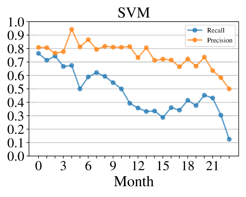
(a)

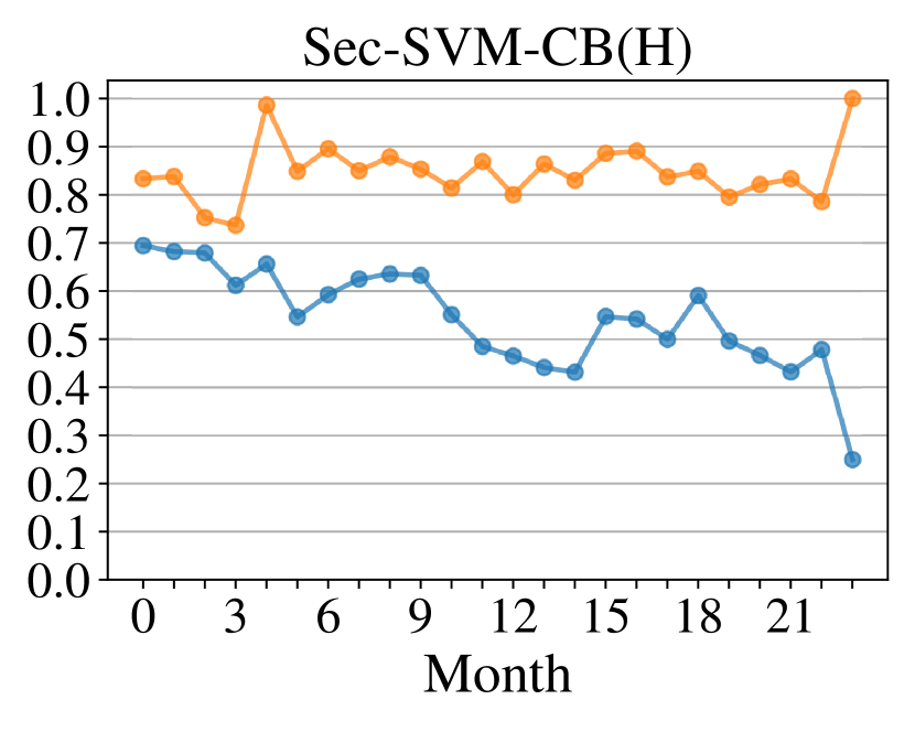
(b)

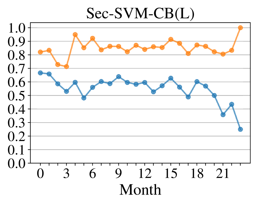
(c)

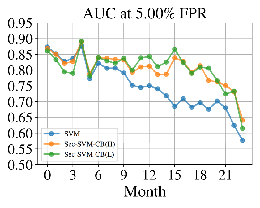
(d)

Figure 4: The precision (orange) and recall (blue) of SVM (a), SVM-CB (H) (b) and SVM-CB (L) (c), and the Area Under the ROC curves (AUC) at 5% (d) for the three classifiers over the 2-years testing periods (from Jan-2015 to Dec-2016).

0.5 Related Work

We now offer an overview of state-of-the-art techniques similar to our proposal. Pendlebury et al. [8] proposes Tesseract, a test-time evaluation framework to determine the faultiness of classifiers in the presence of the concept-drift. The authors show that evaluations are affected by misleading biases that inject artifacts inside the trained machine learning model, thus causing a performance decay once the model faces real-world data. Tesseract highlights how different proposed models do not cope with the concept drift of Android applications and that faulty training settings inflated their original evaluations. While Tesseract is a consistent method to include concept drift in the evaluation, it is not designed to either fix or mitigate its presence.

Jordaney et al. [10], propose Transcend, a framework that signals the premature aging of classifiers before their performance starts to degrade consistently by analyzing the difference between samples observed at training at test time. On top of this methodology, Barbero et al. [11] propose Transcendent, which improves Transcend to include the rejection of out-of-distribution samples that cause the performance drops. However, they do not propose methods to harden a classifier against concept drift, rather they focus on protection systems exploiting samples encountered during deployment, such as a notification when data start differing from the training one [10], or directly rejecting a sample coming from a drifted data distribution [11].

In contrast to previous work, we consider the presence of faulty evaluations, and we extend it with a methodology that quantifies which features of the data distributions are changing and how. Such contribution not only explains the performance decay, but also helps understanding the reasons behind the concept drift. Instead of rejecting samples or just signaling the worsening of the performances of a model, we build a time-aware classifier that takes into account the acquired knowledge of the data distribution changes, and we show how our methodology can better withstand the passing of time.

0.6 Conclusions and Future Work

In this work, we propose a preliminary methodology that understands and provide an initial hardening against the concept drift that plagues the performance of Android malware detection. In particular, we develop a drift-analysis framework that highlights which features contribute more to the performance decay of a classifier over time, and we leverage these results to propose SVM-CB, a linear classifier hardened against the passing of time.

We show the efficacy of our proposals by applying our drift-analysis framework to Drebin, a linear Android malware detector, and we compare its performances over time against its hardened version computed through our proposed methodology. From our experimental analysis, we can precisely detect which features worsen the detection rate of Drebin and how the trained SVM-CB better withstand the passing of time. In particular, we highlight the efficacy of the bounding of these unstable features, reducing the performance drop of SVM-CB w.r.t. the baseline Drebin.

Although the obtained results are promising, this work presents the following limitations. First, the experimental setup does not guarantee that the provided solution against performance decay can be applied to other types of detectors, as this work addresses the problem of analyzing the effect of the concept drift only for linear classifiers that work only on static features [1, 16]. Also, the T-stability might not reflect the actual concept drift that affects Android applications, as it is computed on a classifier trained on a specific dataset, which approximates the real data distribution. Hence, we should also study the Android malware domain more to provide sufficient and reliable evidence of why the features chosen by the drift-analysis framework are actually causing the decay. Lastly, we heuristically tuned the bounds for the selected weights of SVM-CB, but these choices could be improved with an automatic algorithm that computes the ones that lead to better robustness against time.

However, we anyhow believe that our work can suggest a promising research direction that will provide more insight on the usage of each contribution. We first intend to explore more advanced methods based on the drift-analysis framework, including an automatic bound selection for the weights inside the learning algorithm, by adopting a regularization term tailored specifically for temporal performance stability. Secondly, we intend to generalize this method to address deep learning algorithms, where the feature extractor and the feature representation of the last linear layer evolve during training.

Moreover, we will explore other research directions, such as (i) the quantification and prevention of machine learning malware detectors from forgetting old threats when updated with new data, and (ii) the inclusion of research fields such as Continual Learning,  which model data as a continuous stream, thus enabling the development of techniques for updating classifiers constantly and effortlessly.

References

- [1] Daniel Arp, Michael Spreitzenbarth, Malte Hubner, Hugo Gascon, Konrad Rieck, and CERT Siemens. Drebin: Effective and explainable detection of android malware in your pocket. In Ndss, volume 14, pages 23–26, 2014.
- [2] Enrico Mariconti, Lucky Onwuzurike, Panagiotis Andriotis, Emiliano De Cristofaro, Gordon Ross, and Gianluca Stringhini. Mamadroid: Detecting android malware by building markov chains of behavioral models, 2017.
- [3] Kathrin Grosse, Nicolas Papernot, Praveen Manoharan, Michael Backes, and Patrick McDaniel. Adversarial examples for malware detection. In European symposium on research in computer security, pages 62–79. Springer, 2017.
- [4] Milad Taleby Ahvanooey, Qianmu Li, Mahdi Rabbani, and Ahmed Raza Rajput. A survey on smartphones security: software vulnerabilities, malware, and attacks. arXiv preprint arXiv:2001.09406, 2020.
- [5] Alireza Souri and Rahil Hosseini. A state-of-the-art survey of malware detection approaches using data mining techniques. Human-centric Computing and Information Sciences, 8(1):1–22, 2018.
- [6] Abdelfattah Amamra, Chamseddine Talhi, and Jean-Marc Robert. Smartphone malware detection: From a survey towards taxonomy. In 2012 7th International Conference on Malicious and Unwanted Software, pages 79–86. IEEE, 2012.
- [7] Geoffrey I Webb, Roy Hyde, Hong Cao, Hai Long Nguyen, and Francois Petitjean. Characterizing concept drift. Data Mining and Knowledge Discovery, 30(4):964–994, 2016.
- [8] Feargus Pendlebury, Fabio Pierazzi, Roberto Jordaney, Johannes Kinder, and Lorenzo Cavallaro. TESSERACT: Eliminating experimental bias in malware classification across space and time. In 28th USENIX Security Symposium (USENIX Sec. 19), pages 729–746, 2019.
- [9] Anshuman Singh, Andrew Walenstein, and Arun Lakhotia. Tracking concept drift in malware families. In Proceedings of the 5th ACM workshop on Security and artificial intelligence, pages 81–92, 2012.
- [10] Roberto Jordaney, Kumar Sharad, Santanu K Dash, Zhi Wang, Davide Papini, Ilia Nouretdinov, and Lorenzo Cavallaro. Transcend: Detecting concept drift in malware classification models. In 26th USENIX Security Symposium (USENIX Sec. 17), pages 625–642, 2017.
- [11] Federico Barbero, Feargus Pendlebury, Fabio Pierazzi, and Lorenzo Cavallaro. Transcending transcend: Revisiting malware classification in the presence of concept drift. arXiv preprint arXiv:2010.03856, 2020.
- [12] Donghui Hu, Zhongjin Ma, Xiaotian Zhang, Peipei Li, Dengpan Ye, and Baohong Ling. The concept drift problem in android malware detection and its solution. Security and Communication Networks, 2017, 2017.
- [13] Annamalai Narayanan, Liu Yang, Lihui Chen, and Liu Jinliang. Adaptive and scalable android malware detection through online learning. In 2016 International Joint Conference on Neural Networks (IJCNN), pages 2484–2491. IEEE, 2016.
- [14] Corinna Cortes and Vladimir Vapnik. Support-vector networks. Machine learning, 20(3):273–297, 1995.
- [15] Kevin Allix, Tegawendé F Bissyandé, Jacques Klein, and Yves Le Traon. Androzoo: Collecting millions of android apps for the research community. In 2016 IEEE/ACM 13th Working Conference on Mining Software Repositories (MSR), pages 468–471. IEEE, 2016.
- [16] Ambra Demontis, Marco Melis, Battista Biggio, Davide Maiorca, Daniel Arp, Konrad Rieck, Igino Corona, Giorgio Giacinto, and Fabio Roli. Yes, machine learning can be more secure! a case study on android malware detection. IEEE Transactions on Dependable and Secure Computing, 16(4):711–724, 2017.