Global Evaluation for Decision Tree Learning

Abstract

We transfer distances on clusterings to the building process of decision trees, and as a consequence extend the classical ID3 algorithm to perform modifications based on the global distance of the tree to the ground truth—instead of considering single leaves. Next, we evaluate this idea in comparison with the original version and discuss occurring problems, but also strengths of the global approach. On this basis, we finish by identifying other scenarios where global evaluations are worthwhile.

1 Decision Tree Learning

The classification problem in machine learning asks, given some observed instances with known outcomes (called the labeled training data), to make predictions on outcomes of unseen instances.

Formally, let $\Omega$ be a universe of instances. Every $x\in\Omega$ has attributes $x_{1},\dots,x_{m}\in\mathbb{R}$. Outcomes of instances in the training set $X\subseteq\Omega$, also called class labels, are given by a map $y:\Omega\to\{1,\dots,k\}$. One popular choice of a model to train is the decision tree. We restrict our analysis to binary decision trees; binary trees whose branches consist of splitting criteria $c:\Omega\to\{0,1\}$ and whose leaves are class labels $\{1,\dots,k\}$. The decision tree models a discrete-valued function. Every instance $x$ is sorted down the decision tree by evaluating branch predicates $c$ and recursing into the respective subtree: left if $c(x)=0$ and right if $c(x)=1$. Once a leaf is encountered, its class label is returned. Decision trees are capable of handling continuous and discrete attributes and hence a multitude of splitting criteria are commonly used. Here we restrict ourselves to binary criteria of the form $c(x)=[x_{j}\leq r]$ for an attribute $j$ and limit $r\in\mathbb{R}$.

The labels $y$ can also be interpreted as a clustering $\mathcal{Y}=(Y_{1},\dots,Y_{k})$ where every cluster set is defined as $Y_{i}=y^{-1}(i)=\{\,{x\in X\mid y(x)=i}\,\}$. Hence, we will use $y$ and $\mathcal{Y}$ interchangeably. A decision tree $t$ naturally induces a clustering on X as well, denoted by $\mathcal{T}_{t}$. This leads to the idea to utilize distances on clusterings in the construction process of decision trees.

1.1 Distances between Clusterings

To keep the following definitions concise, we denote the set of all $k$-clusterings on $X$ as $\left\{\begin{subarray}{c}X\\ k\end{subarray}\right\}=_{\rm def}\{\,{(A_{1},\dots,A_{k})\mid A_{1}\;\dot{\cup}\;\cdots\;\dot{\cup}\;A_{k}=X}\,\}$ and write $A\circ\mathcal{B}=_{\rm def}(A\circ B_{1},\dots,A\circ B_{l})\in\left\{\begin{subarray}{c}A\circ X\\ l\end{subarray}\right\}$ as well as $\mathcal{A}\circ\mathcal{B}=_{\rm def}(A_{1}\circ B_{1},\dots,A_{i}\circ B_{j},\dots,A_{k}\circ B_{l})\in\left\{\begin{subarray}{c}X\circ X\\ k\cdot l\end{subarray}\right\}$ for clusterings $\mathcal{A}\in\left\{\begin{subarray}{c}X\\ k\end{subarray}\right\},\mathcal{B}\in\left\{\begin{subarray}{c}X\\ l\end{subarray}\right\}$, a set $A\subseteq X$, and an operation $\circ$ on $\mathcal{P}(X)$. We call a clustering $\mathcal{A}$ trivial if $A_{i}=X$ for an $i\in\{1,\dots,k\}$.

In the following, let clusterings $\mathcal{A}$ and $\mathcal{B}$ be defined as above. We understand a real-valued function $f:\left\{\begin{subarray}{c}X\\ k\end{subarray}\right\}^{2}\to\mathbb{R}$ as a gdistance measure if $f(\mathcal{A},\mathcal{B})$ decreases with $\mathcal{A}$ and $\mathcal{B}$ becoming more similar, and as a gsimilarity measure if $f(\mathcal{A},\mathcal{B})$ increases. We always refer to measures as distance measures, sometimes implying that a similarity measure has to be inverted. All introduced measures are summarized along with their properties in Table 1, and a more complete collection of distance measures on clusterings can be found in [7]. The first distance measures we introduce originate in probability theory.

Information-Theoretic Measures

For subsets $A,B\subseteq X$, define

$$P(A)=_{\rm def}\dfrac{|A|}{|X|}=\mathbf{P}\!\left[\,{x\in A}\,\right],\hskip 14.22636ptP(A|B)=_{\rm def}\dfrac{P(A\cap B)}{P(B)}=\dfrac{|A\cap B|}{|B|}=\mathbf{P}\!\left[\,{x\in A\mid x\in B}\,\right]$$

where $x$ is a random variable assuming values from $X$ uniformly at random. Understanding a clustering $\mathcal{A}$ as a probability distribution $P(A_{i})$ over values of $i$ allows us to transfer probability-theoretic concepts to clusterings: the (Shannon) gentropy associated with a clustering $\mathcal{A}$ and the gexpected conditional entropy of a clustering $\mathcal{A}$ given $\mathcal{B}$ are defined as:

$$\begin{array}[]{rrl}\mathrm{H}(\mathcal{A})&=_{\rm def}&-\sum_{i=1}^{k}P(A_{i})\log P(A_{i})\\[3.0pt] \displaystyle\mathrm{H}(\mathcal{A}\mid\mathcal{B})&=_{\rm def}&\mathbf{E}_{j}\!\left[\,\mathrm{H}(\mathcal{A}\mid B_{j})\,\right]~{}=_{\rm def}~{}-\sum_{i=1}^{k}\sum_{j=1}^{l}P(A_{i}\cap B_{j})\log P(A_{i}\mid B_{j})\end{array}$$

Clearly, $\mathrm{H}(\mathcal{A}|\mathcal{B})=\mathrm{H}(\mathcal{A}\cap\mathcal{B})-\mathrm{H}(\mathcal{B})$.

The gKullback-Leibler divergence associated with $\mathcal{C}\in\left\{\begin{subarray}{c}X\\ k\end{subarray}\right\}$ and $\mathcal{C}^{\prime}\in\left\{\begin{subarray}{c}Z\\ k\end{subarray}\right\}$ is the relative entropy between $P(C_{i})$ and $P(C^{\prime}_{i})$, given as

$$D_{\mathrm{KL}}(\mathcal{C}\,\|\,\mathcal{C}^{\prime})=_{\rm def}\sum_{i=1}^{m}P(C_{i})\log\frac{P(C_{i})}{P(C^{\prime}_{i})}\ .$$

This definition is not yet suited to compare clusterings as it does not consider their joint distributions. Instead, we measure the divergence of the joint distribution $P(A_{i}\cap B_{j})$ to its independent counterpart $P(A_{i})P(B_{j})$: The gmutual information between two clusterings $\mathcal{A}$ and $\mathcal{B}$ is defined as

$$\begin{array}[]{l}\displaystyle\mathrm{I}(\mathcal{A},\mathcal{B})=_{\rm def}D_{\mathrm{KL}}(\mathcal{A}\cap\mathcal{B}\,\|\,\mathcal{A}\times\mathcal{B})=\sum_{i=1}^{k}\sum_{j=1}^{l}P(A_{i}\cap B_{j})\log\frac{P(A_{i}\cap B_{j})}{P(A_{i})P(B_{j})}\\[15.0pt] \hskip 113.81102pt=\mathbf{E}_{j}\!\left[\,D_{\mathrm{KL}}(\mathcal{A}\cap B_{j}\,\|\,\mathcal{A})\,\right]=\mathrm{H}(\mathcal{A})-\mathrm{H}(\mathcal{A}\mid\mathcal{B})~{}_{\rm def}=\mathrm{Gain}(\mathcal{A},\mathcal{B})\end{array}$$

and also known as ginformation gain in the context of decision tree learning [5, p. 58].

The gvariation of information (VI) is given as $\mathrm{VI}(\mathcal{A},\mathcal{B})=_{\rm def}\mathrm{H}(\mathcal{A}\mid\mathcal{B})+\mathrm{H}(\mathcal{B}\mid\mathcal{A})$. A normalized version

$$\mathrm{VI}_{\mathrm{n}}(\mathcal{A},\mathcal{B})=_{\rm def}\dfrac{\mathrm{VI}(\mathcal{A},\mathcal{B})}{\mathrm{H}(\mathcal{A}\cap\mathcal{B})}=1-\dfrac{\mathrm{Gain}(\mathcal{A},\mathcal{B})}{\mathrm{H}(\mathcal{A}\cap\mathcal{B})}$$

can also take the shape of a normalized information gain [1]. Previously, the ginformation gain ratio defined as

$$\mathrm{GainRatio}(\mathcal{A},\mathcal{B})=_{\rm def}\frac{\mathrm{Gain}(\mathcal{A},\mathcal{B})}{H(\mathcal{B})}\ .$$

was proposed as normalization [6]. Other normalizations take the geometric or arithmetic mean based on the fact that $\mathrm{I}(\mathcal{A},\mathcal{B})\leq\min\{\mathrm{H}(\mathcal{A}),\mathrm{H}(\mathcal{B})\}$.

Gini Impurity

Let the gGini impurity [8] be defined as

$$\mathrm{Gini}(\mathcal{A},\mathcal{B})=_{\rm def}\sum_{j=1}^{l}P(B_{j})\left(1-\sum_{i=1}^{k}P(A_{i}|B_{j})^{2}\right)=1-\sum_{j=1}^{l}\frac{1}{P(B_{j})}\sum_{i=1}^{k}P(A_{i}\cap B_{j})^{2}\ .$$

Jaccard Distance

For a nonnegative, monotone, and submodular set function $f$ on $X$, let the distance $D_{f}:\mathcal{P}(X)\to\mathbb{R}$ be defined as

$$D_{f}(\mathcal{A},\mathcal{B})=_{\rm def}\sum_{i=1}^{k}J_{f}(A_{i},B_{i})=\sum_{i=1}^{k}\frac{f(A_{i}\triangle B_{i})-f(\emptyset)}{f(A_{i}\cup B_{i})}$$

where $A\triangle B=(A\cup B)\setminus(A\cap B)$ denotes the symmetric difference between $A$ and $B$. $D_{f}$ is a metric distance function being the sum of $k$ metric distance functions $J_{f}$ [4]. For the cardinality $f(A)=|A|$, we obtain the gextended Jaccard distance

$$D_{|\cdot|}(\mathcal{A},\mathcal{B})=k-\sum_{i=1}^{k}\frac{P(A_{i}\cap B_{i})}{P(A_{i}\cup B_{i})}\ .$$

Accuracy

Finally, we define the prediction accuracy of clustering $\mathcal{B}$ for clustering $\mathcal{A}$ as

$$\mathrm{acc}(\mathcal{A},\mathcal{B})=_{\rm def}\frac{1}{|X|}\sum_{i=1}^{k}|A_{i}\cap B_{i}|=\sum_{i=1}^{k}P(A_{i}\cap B_{i})\ .$$

The following table summarizes the measures together with some properties.

	Measure		Range	Permutationinvariant	Metric
⚫	Information Gain	$\mathrm{Gain}(\mathcal{A},\mathcal{B})$	$[0,\infty]$	✓	✗
⚫	Gain Ratio	$\mathrm{GainRatio}(\mathcal{A},\mathcal{B})$	$[0,1]$	✓	✗
▲	normalized VI	$\mathrm{VI}_{\mathrm{n}}(\mathcal{A},\mathcal{B})$	$[0,1]$	✓	✓
▲	Gini Impurity	$\mathrm{Gini}(\mathcal{A},\mathcal{B})$	$[0,1]$	✓	✗
▲	extended Jaccard	$D_{|\cdot|}(\mathcal{A},\mathcal{B})$	$[0,k]$	✗	✓
▲	inverted Accuracy	$1-\mathrm{acc}(\mathcal{A},\mathcal{B})$	$[0,1]$	✗	✓

Table 1: Overview of distance measures. The first row shows whether a function is a distance (▲) or a similarity (⚫) measure. All functions are symmetric, i.e., $\Delta(\mathcal{A},\mathcal{B})=\Delta(\mathcal{B},\mathcal{A})$. A function is called permutation invariant if $\Delta(\mathcal{A},\mathcal{B})=\Delta((A_{\sigma(1)},\dots,A_{\sigma(k)}),\mathcal{B})$ for all $\sigma\in S_{k}$.

1.2 Local Distance Evaluation: ID3

The most common algorithm for decision tree learning is the greedy top-down optimizer ID3 [6], shown in Algorithm 2.

We describe decision trees algebraically using $\mathrm{Branch}(c,t_{1},t_{2})$ to denote a tree with splitting criterion $c:\Omega\to\{0,1\}$ and $t_{1}$ and $t_{2}$ as left and right subtrees. A leaf of class $i\in\{1,\dots,k\}$ is indicated as $\mathrm{Leaf}(i)$ and the subset of all instances in the training set $X$ sorted down along the tree into a leaf $v$ are denoted as $\mathrm{instances}(t,v)$. A leaf is called pure if $|y(\mathrm{instances}(t,v))|\leq 1$ and a splitting criterion $c$ is called valid (regarding a set of instances $X^{\prime}=\mathrm{instances}(t,v)$ in a leaf $v$) if $c|_{X^{\prime}}$ is non-trivial. Finally, during tree construction, $\mathrm{exchange}(t,v,t^{\prime})$ is the tree resulting from replacing $v$ in $t$ by $t^{\prime}$.

Algorithm 2: ID3

Input: Training data $(X,y)$ and distance measure $\Delta$

Output: Decision tree $t$

$t\leftarrow\text{empty tree}$

while $\mathcal{T}_{t}\not=\mathcal{Y}$ do

       $(v,X^{\prime},c)\leftarrow\operatorname*{arg\,min}\{\;\Delta(c|_{X^{\prime}},y|_{X^{\prime}})\mid\textrm{impure leaves $v$ of $t$},\,\textrm{$X^{\prime}=\mathrm{instances}(t,v)$,}$

                                                       $\textrm{valid splitting critera $c$}\;\}$

       for $b\in\{0,1\}$ do

             $i_{b}\leftarrow\operatorname*{arg\,max}\{\,{|(c|_{X^{\prime}})^{-1}(b)\cap y^{-1}(i)|\mid i\in\{1,\dots,k\}}\,\}$

            

      $t\leftarrow\mathrm{exchange}(t,v,\mathrm{Branch}(c,\mathrm{Leaf}(i_{0}),\mathrm{Leaf}(i_{1})))$

      

return $t$

ID3 starts with an empty tree and grows the tree in every iteration by replacing a leaf with a new branch containing a splitting criterion and two leaves itself. The leaf to replace and the splitting criterion $c$ are determined by evaluating the distance measure $\Delta$ on the instances in every leaf as clustered by $y$ and as clustered by $c$. The leaf posing an overall minimum on the distance is selected to be split along the respective splitting criterion. Splitting leaves that are already pure or splitting along a splitting criterion which results in an empty leaf is not allowed to ensure that the algorithm will stop. Finally, the two new leaves get assigned the label which is most prevalent amongst their instances.

Bias-Variance Tradeoff

We briefly consider the following decomposition of the classification error to identify challenges in decision tree learning. The expected error of a regressor $\hat{f}$ for a sample $x\in\Omega$ can be written as

$$\mathbf{E}((y-\hat{f}(x))^{2})=\mathrm{Bias}(\hat{f}(x))^{2}+\mathrm{Var}(\hat{f}(x))+\sigma^{2}\quad\textrm{where}\quad\mathrm{Bias}(\hat{f}(x))=_{\rm def}\mathbf{E}(\hat{f}(x))-f(x)$$

assuming $y=f(x)+\varepsilon$ is a noisy sample of the original distribution $f$ with $\varepsilon\sim{\cal N}(0,\sigma^{2})$. This motivates the idea to average multiple independent classifiers $\hat{f}_{1},\dots,\hat{f}_{s}$ as we obtain $\mathrm{Var}(1/s\cdot\sum_{i=1}^{s}\hat{f}_{i}(x))=1/s\cdot\mathrm{Var}(\hat{f}(x))$, assuming equal variance for all regressors. We train each classifier on a sample drawn with replacement from the training set. Training on small samples increases the bias of the final classifier, but for strong learners that adapt arbitrarily well to the training data (such as decision trees), this is a valuable trade-off.

A similar decomposition of the expected error exists for a classification task [2]; instead of averaging multiple classifiers, we take the mode and obtain a random forest. Now, consider a dataset that originates from a decision tree. Here, we also have a concept of bias and variance in tree structure: How similar is a tree created by the learning algorithm to the original on average, and how much deviate learned trees from each other. These ideas correspond closely to the notions of bias and variance defined above.

Another common way to balance this equation is by pruning. Techniques such as early stopping limit the tree height or the minimum number of instances per leaf. This increases the bias but on the other hand, prevents the tree from overfitting and thus lowers its variance.

1.3 Global Distance Evaluation

We now want to explore a strategy that still grows the tree by performing local modifications, but decides on them based on evaluations of a distance measure on the whole training set, not only on the instances in a single leaf (see Algorithm 3). We call this gglobal evaluation.

Algorithm 3: ID3 with Global Evaluation

Input: Training data $(X,y)$ and distance measure $\Delta$

Output: Decision tree $t$

$t\leftarrow\text{empty tree}$

while $\mathcal{T}_{t}\not=\mathcal{Y}$ do

       $t^{\prime}\leftarrow\operatorname*{arg\,min}\{\;\Delta(\mathcal{T}_{t^{\prime}},\mathcal{Y})\mid\textrm{impure leaves $v$ of $t$},\,\textrm{valid splitting critera $c$},$

                                         $\textrm{class labels $i_{0},i_{1}\in\{1,\dots,k\}$},$

                                         $t^{\prime}=\mathrm{exchange}(t,v,\mathrm{Branch}(c,\mathrm{Leaf}(i_{0}),\mathrm{Leaf}(i_{1})))\;\}$

       $t\leftarrow t^{\prime}$

return $t$

In classical ID3 we evaluate our distance measures between clusterings on the instances in the current leaf, namely the 2-clustering given by the splitting criterion and the clustering given by the ground truth $y$. To evaluate globally, we have to decide on the labels $i_{0},i_{1}$ assigned to both sides of the split beforehand. Algorithm 3 evaluates the distance measure on all combinations of class labels and decides for the one inducing the minimum distance. A more efficient strategy is to assign the most prevalent class.

2 Evaluation

   Information Gain Gini Impurity extended Jaccard normalized VI Iris (150s, 4f, 3c) Cardiotocography (2126s, 13f, 3c) Natural Data Wine (178s, 13f, 3c) Gaussian Blobs (2000s, 3f, 3c) Monks (556s, 6f, 2c) Monks 2 (602s, 6f, 2c) Artificial Data Monks 3 (554s, 6f, 2c) Figure 4: The plot shows test accuracies and tree sizes of decision trees. Each column corresponds to one distance measure, each row to one dataset. Every cell shows statistics for both the global and the local version of ID3 (where the global version is always shown in red). The continuous line corresponds to the accuracy of the tree as evaluated on a test set consisting of 10% of the data. On the x-axis is the size of the train set drawn without replacement from the remaining 90% of the data. The tree size is indicated by the dashed line and surrounded by its confidence interval. Every training process was repeated 500 times to ensure significance.

After introducing the most common distance measures and the two versions of ID3, we turn towards the evaluation of their performance. We use the Monks, Wine, Cardiotocography, and Iris datasets from the UCI Machine Learning Repository [9] and isotropic Gaussian blobs.

2.1 Test Accuracy and Tree Size

Typical evaluation criteria after training of a classification algorithm are train and test accuracy. Both values can tell us whether our classificator is over- or underfitted. As we ignore pruning for now, which means the trained trees always fit perfectly to the training data, we can only evaluate how overfitted the tree is through the test accuracy.

Now, consider a scenario where a decision tree is trained on data directly sampled from another tree. Of course, a good decision tree would not only achieve high accuracy but also resemble the original tree as closely as possible. This makes sense as such an estimator achieves low bias on the tree structure, and hence generalizes better on unseen data. Also, decision trees are sought to be humanly interpretable for gaining insights into the given data. If the data is in fact not sampled from a tree, it is still worthwhile to uncover an approximate hidden tree structure, though it is unclear what this looks like. As such, we always consider the number of nodes as a measure of tree size in our evaluation.

Findings

We can see these properties in Figure 4 for several artificial and natural datasets along with the distance measures that were generating the best results for both local and global evaluation, namely information gain, Gini impurity, the extended Jaccard distance, and the normalized variation of information. The trees were trained on increasing sample sizes, to simulate scenarios where the structure in the data is over- or under-represented by a sample.

Generally, there is a discrepancy between artificial and natural data. Global and local evaluation perform similarly on natural data. Only trees grown with the extended Jaccard distance on the Iris dataset overfit the data which results in high tree size and variance thereof. We also observe that the global evaluation outperforms local evaluation on small training sets.

The situation changes when looking at the four artificial datasets. Only when using Gini impurity do both classifiers perform equally well, otherwise, local evaluation achieves higher accuracy and lower tree size. However, using the extended Jaccard distance in the Monks 1 dataset is superior to all other distance measures, in particular when evaluated globally. Though on Gaussian Blobs and Monks 3, the extended Jaccard distance fails if evaluated globally.

Overall, we note that low tree size goes in hand with good accuracy. A tree of lower complexity does not necessarily represent the data better [5, p. 65], but judging from our evaluation, this is empirically correct. In the next section, we will look into minimal representations in more detail.

2.2 Tree Size on Artificial Data

Information Gain

Gain Ratio

normalized VI

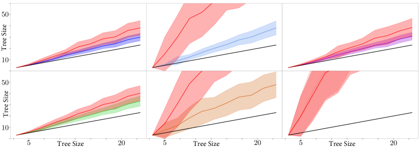
Gini Impurity

extended Jaccard

Accuracy

Figure 5: Mean tree size and standard deviation of decision trees created by global and local evaluation. Again, the globally learned trees appear in red. The y-axis (and the black line) shows the minimum tree size necessary to represent a certain sample of 500 vectors with 6 features of 4 classes. Experiments for every tree size were repeated 200 times.

Given a sample $(X,y)$, a tree is gconsistent if it classifies all data points in $X$ correctly and gminimal if its number of nodes is minimum among all consistent trees. In Figure 5, we evaluate the tree size of classifiers with respect to the size of the tree the training data was sampled from, by showing the number of nodes in a tree. Trees and samples are randomly generated, but discarded if one classifier finds a consistent tree that is smaller than the original. This ensures that the original trees are minimal for the produced samples and we get a better estimate of how close a classifier is to the original.

Global evaluation generates larger trees for every distance measure. Local evaluation of information gain, normalized variation of information, and Gini impurity generates the smallest trees and global evaluation of these distance measures is not much worse. The global versions of all other algorithms create unnecessarily large trees. However, the given data is heavily biased and we already saw in Figure 4 that an algorithm’s performance depends on the distribution it is sampled from, and in particular whether that is natural or artificial.

3 Problems

The above results may seem contradictory. We chose local manipulations to a tree $t$ to decrease the distance between $\mathcal{T}_{t}$ and the ground truth $\mathcal{Y}$ in a greedy fashion. In the end, we want the distance to vanish, i.e., achieve equal clusters. Should global evaluation not result in faster convergence of $\mathcal{T}_{t}$ towards $\mathcal{Y}$ as local evaluation, since it considers all instances in every step? Also, should accuracy as a simple measure of deviance from equality not deliver the best results? We will try to find reasons in the following.

3.1 Minimal Trees

Although finding minimal trees is NP-complete [3], we can find such a tree using the greedy ID3 algorithm with the following distance measure. Define

$$\begin{array}[]{l}\mathrm{mts}(\mathcal{C})=_{\rm def}\min\{\,{\mathrm{size}(t)\mid\textrm{decision tree $t$ with $\mathcal{T}_{t}=\mathcal{C}$}}\,\}\quad\textrm{and}\\ \hskip 180.00027pt\Delta_{\textrm{mts}}(\mathcal{A},\mathcal{B})=_{\rm def}\sum_{i=1}^{k}\mathrm{mts}(A_{i}\cap\mathcal{B})\end{array}$$

where $\mathrm{size}(t)$ is the number of nodes in $t$. Note that unlike previous distance measures, this is an internal measure looking into attributes of the vectors $x\in X$, rather than solely class labels. Using this distance in the locally evaluating version of ID3 results in a minimal tree. Growing the tree according to global evaluations of any distance measure inevitably fails to produce minimal trees as the clustering $\mathcal{T}_{t}$ is agnostic of the tree structure.

We can understand $\mathrm{mts}(\mathcal{Y})$ as a measure of complexity in the clustering $\mathcal{Y}$ and, for example, the entropy $\mathrm{H}(\mathcal{Y})$ as an efficiently-computable estimator thereof. The above construction suggests that using a distance measure $\Delta((A_{1},\dots,A_{k}),\mathcal{Y})$ which is an aggregate of the approximate clustering complexities in $A_{i}\cap\mathcal{Y}$ leads to short trees.

3.2 Redundant Splitting

A redundant split occurs if the generated tree contains a subtree of the form

$$\mathrm{Branch}(c_{1},\mathrm{Leaf}(i),\mathrm{Branch}(c_{2},\mathrm{Leaf}(i),t))$$

where $c_{1}(x)=[x_{j}\leq r_{1}]$ and $c_{2}(x)=[x_{j}\leq r_{2}]$ for a common feature $j\in\{1,\dots,m\}$, class label $i\in\{1,\dots,k\}$, and subtree $t$. The same classification can be achieved by a smaller tree $\mathrm{Branch}(c,\mathrm{Leaf}(i),t)$ with $c(x)=[x_{j}\leq\max\{r_{1},r_{2}\}]$. Redundant splits can occur during decision tree building if every split trough the instances of a leaf increases the distance to the ground truth. ID3 will then choose to split along a plane having fewest instances on one side, thus altering the current clustering $\mathcal{T}_{t}$—and decreasing the distance—only slightly.

(a) Local evaluation

Measure	(L)	(G)
information gain	✓	✗
gain ratio	✓	✗
normalized VI	✓	✗
Gini impurity	✓	✗
extended jaccard	✗	✗
inverted accuracy	✗	✗

(c) Efficient splits

(b) Global evaluation

Figure 6: Classification surface for local and global optimization. The colored dots represent the ground truth $\mathcal{Y}$ whereas the background-color represents the clustering induced by the decision tree being built. Introducing a leaf that splits at $c_{2}$ leads to a redundant split while splitting at $c_{1}$ is the most efficient split, making fastest progress towards a consistent tree; (c) shows which distance measure induces an efficient split, in both the local (L) and global (G) setting.

Figure 6 shows two settings, a local and a global one, in which redundant splits can occur. It turns out that all distance measures are susceptible to redundant splitting when evaluated globally. Using the extended Jaccard distance and inverted accuracy also exhibit behavior this when evaluated locally.

4 Pruning and Glocal Evaluation

In the previous sections, we discussed that global evaluation generally creates trees with lower test accuracy and higher tree size than local evaluation. This is due to a higher bias of the ID3 algorithm using global evaluation which overgrows most trees. However, in a scenario with small sample size or an overly noisy sample, we benefit from an increased bias. The former was already apparent in Section 2, so we will discuss the latter in this final section. Since both local and global evaluation fit arbitrarily well to the training data, we have to employ pruning strategies to prevent overfitting.

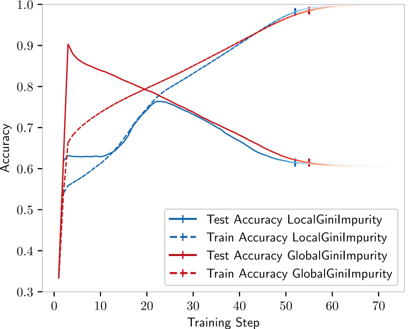
(a) No pruning (Gini impurity)

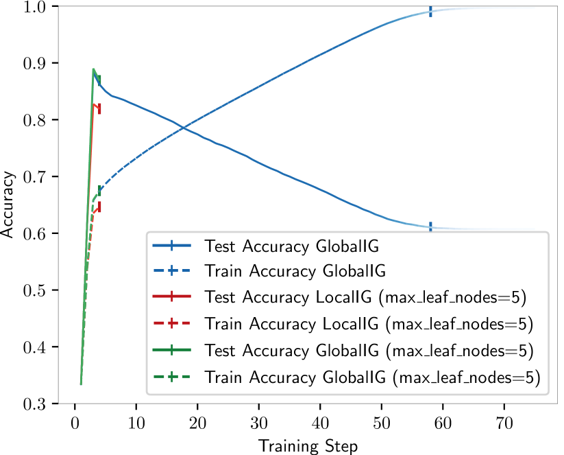
(b) Limit on the number of nodes (information gain)

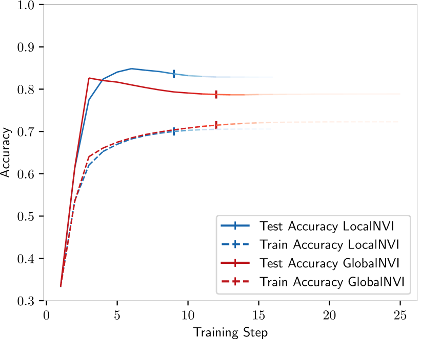
(c) Requiring a minimum of instances in each branch (normalized variation of information)

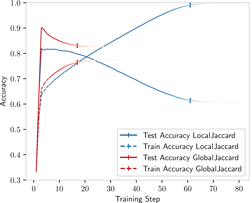
(d) No distance decay (extended Jaccard distance)

Figure 7: Classification accuracy during training on noisy data using different pruning techniques. The data was obtained by assigning random classes for 50% of the instances of the Iris dataset. The dashed line indicates the train accuracy on the noisy data, while the solid line indicates the test accuracy on the original data. The training process was repeated 1000 times and averaged. The opacity shows the percentage of unfinished trees in each step and the horizontal tick marks where the majority of trees finished training.

In Figure 7, we see average train and test accuracies of a tree during its construction, as well as the average final train and test accuracy. We discuss different pruning strategies in the following.

1. gNo pruning: The test accuracy spikes in the early training steps of the globally evaluating version. However, the tree quickly overfits and the test accuracy of both versions of the algorithm decays to around 60%. This is almost inevitable without pruning for training data with such high noise.

2. gLimit on the number of nodes: The most basic idea is to stop training after a certain number of steps, i.e., limit the number of nodes. We can stop training when the test accuracy spikes, but in practice, it is hard to estimate this point. The global approach reached a higher peak in 1, hence seems favorable for this kind of pruning. One reason for this is that local evaluation prioritizes splits improving a leaf the most, possibly ignoring a split through a leaf that would lead to many more instances being classified accurately. Another reason is that local evaluation recurses quickly into small sub-samples, where the algorithm becomes more sensitively towards noise.

3. gRequiring a minimum of instances in each branch: Other common techniques are requiring a minimum number of instances in either leaf nodes ore branches. In this example, we require a minimum of 30 instances in a leaf to perform a further split, giving splits more statistic significance. We avoid the previous problem of the local evaluation reacting sensitive towards noise. And in fact, trees with this bias perform better, whereas local evaluation outperforms global evaluation.

4. gNo distance decay: A parameterless pruning strategy is to stop training once every possible split would result in an increased distance. This works out well in our example, but there is a risk to already stop training in a local minimum.

Increasing the bias by pruning only makes sense if the specific bias is actually apparent in the data. Otherwise, we decrease the final accuracy of our classifier. In particular, this means that the success of pruning is highly dependent on the data and distance measure used.

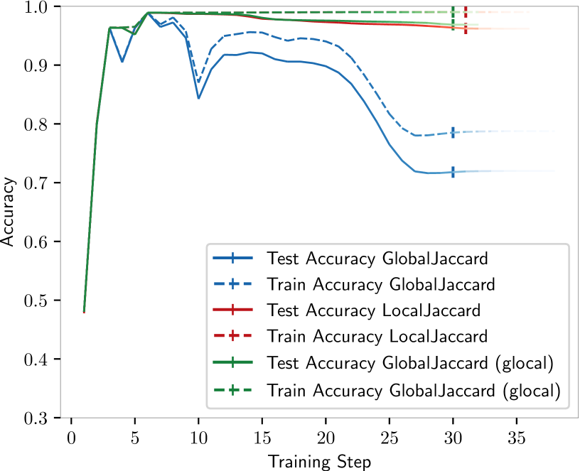
Figure 8: Train (dashed) and test (solid) accuracy during training of a glocal algorithm.

One way to make the classifier applicable to a broader class of datasets is to combine global and local evaluation. In Figure 8, we used an approach that works with global evaluation as long as that decreases the global distance to the ground truth. Otherwise, a step is performed using the original local approach. We observe that this helps to overcome the problems we had using the extended Jaccard distance in the Iris and Monks 3 datasets in Figure 4.

5 Conclusion

After introducing multiple distance measures on clusterings and their application in the ID3 algorithm, we proposed a variation of the algorithm making decisions based on global distance evaluations. We evaluated both approaches and found that using local evaluations generally results in superior accuracy over global evaluations, which often overgrow trees. However, the results are not clear cut and we concluded that the additional bias from larger trees can be useful in scenarios with small sample size or heavy noise, the latter requiring additional pruning. Finally, we also saw how the glocal approach alleviates some difficulties with global evaluation.

We conclude that there is possible application for ID3 under global evaluations, but the performance depends on the scenario on hand. Trees created in this fashion can be useful in data analysis by themselves, or as a random forest, particularly with the shown parameterless pruning strategy.

Acknowledgment: For helpful comments we are grateful to Tobias Sutter (Konstanz).

References

- [1] R. López De Mántaras. A distance-based attribute selection measure for decision tree induction. Machine Learning, 6(1):81–92, 1991.
- [2] P. M. Domingos. A unified bias-variance decomposition and its applications. In Proceedings of the 17th International Confrence on Machine Learning (ICML’2000), pages 231–238. Morgan Kaufmann, 2000.
- [3] T. R. Hancock, T. Jiang, M. Li, and J. Tromp. Lower bounds on learning decision lists and trees. Information and Computation, 126(2):114–122, 1996.
- [4] S. Kosub. A note on the triangle inequality for the Jaccard distance. Pattern Recognition Letters, 120:36–38, 2019.
- [5] T. M. Mitchell. Machine Learning. McGraw-Hill, New York, NY, 1997.
- [6] J. R. Quinlan. Induction of decision trees. Machine Learning, 1(1):81–106, 1986.
- [7] S. Wagner and D. Wagner. Comparing clusterings - an overview. Technical Report IB 2006-4, Fakultät für Informatik, Universität Karlsruhe (TH), Karlsruhe, Germany, 2007.
- [8] L. Breiman, J. H. Friedman, R. A. Olshen, C. J. Stone Classification And Regression Trees. Wadsworth, Belmont, California, 1998.
- [9] D. Dua and C. Graff, C. UCI Machine Learning Repository. Irvine, CA: University of California, School of Information and Computer Science, 2019.