Thermal fluctuations on the freeze-out surface of heavy-ion collisions
and their impact on particle correlations

Abstract

Particle momentum distributions originating from a quark-gluon plasma as produced in high-energy nuclear collisions can be influenced by thermal fluctuations in fluid dynamic fields. We study this effect by generalising the commonly used kinetic freeze-out prescription by allowing for small fluctuations around an average in fluid velocity, chemical potentials and temperature. This leads to the appearance of specific two-body momentum correlations. Combining a blast-wave parametrization of the kinetic freeze-out surface with the thermal correlation functions of an ideal resonance gas, we perform an exploratory study of angular net-charge correlations induced by thermal fluctuations around vanishing chemical potential. We note a diffusion of the near-side peak around $\Delta y=\Delta\phi=0$ induced by variances of different chemical potentials, which could be investigated experimentally.

I Introduction

The phenomenology of ultrarelativistic heavy-ion collisions is centered around the understanding of the evolution of the quark-gluon plasma (QGP) that emerges in the interaction of two nuclei at high energy Braun-Munzinger:2007edi ; Busza:2018rrf . Two decades of experiments have established an effective description of the QGP based on relativistic fluid dynamics Romatschke:2017ejr . The system reaches local thermal equilibrium over a time scale of order 1 fm/$c$ Schlichting:2019abc ; Berges:2020fwq , and it expands as a relativistic fluid for about $10$ fm/$c$ before decoupling to hadrons that eventually freely stream to the detectors.

Fluctuations on top of this picture play a major role in the phenomenology of heavy-ion collisions. They are mainly of two kinds. There are initial-state fluctuations Luzum:2013yya , originating from the fact that the structure of the colliding ions and nucleons fluctuates on an event-by-event basis. They yield, notably, a landscape of peaks and valleys in the created QGP energy density, with nontrivial implications for the subsequent fluid evolution and its signatures. There are, in addition, final-state fluctuations arising from the process of particlization of the fluid, driven by the fact that the QGP decouples to a finite number of hadrons. Of particular interest are the fluctuations of conserved quantities (e.g. baryon number and electric charge), which fluctuate locally, as well as globally within the finite phase-space coverage of the detectors. They might be sensitive to the details of the QGP-hadron transition and potentially to associated critical phenomena Cheng:2008zh ; Fukushima:2010bq ; Bzdak:2019pkr ; Bluhm:2020mpc .

Besides initial- and final-state fluctuations, thermal (or hydrodynamic) fluctuations engendered by the expansion dynamics are also present, in agreement with the dissipation-fluctuation theorem and the fact that the QGP is not a perfect fluid. These fluctuations are the focus of this manuscript. Hydrodynamic fluctuations have been studied in the context of QGP expansion since a long time ago Kapusta:2011gt ; Young:2013fka ; Ling:2013ksb ; Young:2014pka ; Murase:2015oie ; Yan:2015lfa ; Nagai:2016wyx ; Gavin:2016hmv ; Akamatsu:2016llw ; Sakai:2017rfi ; Kapusta:2017hfi ; Chattopadhyay:2017rgh ; Stephanov:2017ghc ; Singh:2018dpk ; Akamatsu:2018vjr ; An:2019osr ; Murase:2019cwc ; An:2019csj ; De:2020yyx ; Sakai:2020pjw ; Chao:2020kcf ; Sakai:2021pev . Their implementation goes typically via the addition of a noise term in the relativistic hydrodynamic equations, and their phenomenological consequences have also been investigated quantitatively.

In this paper, we study how correlation functions of hadrons emerging from the final stages of the QGP are impacted by thermal fluctuations in the fluid fields that describe the system at the intersection between a fluid and a particle description, i.e., on the so-called freeze-out surface. We ask what two-body correlations are engendered in momentum space if one relaxes the common description of the freeze-out surface with unique fluid fields and fixed freeze-out temperature, but takes thermal fluctuations in fluid velocity, chemical potentials and temperature into account.

Our goal is in a sense simpler with respect to previous works, as we shall not aim at evolving thermal fluctuations dynamically over the fluid evolution. We take the standard fluid evolution equations to describe expectation values and to be renormalized in that sense, already. However, our study will permit us to point out generic phenomenological signatures of thermal fluctuations that have not been discussed yet in the literature, and to do so in a simple analytical framework. Our analysis focuses, in particular, on the emergence of differential net-charge fluctuations, depending on transverse momentum and rapidity cuts, which may be straightforwardly measured in experiments.

This manuscript is organized as follows. In Sec. II we briefly recall the physical picture of kinetic freeze-out in heavy-ion collisions, and the formalism adopted to describe it. In Sec. III, we present our main result, namely, the derivation of a relation between two-particle correlations in momentum space arising from the QGP particlization and two-point correlation functions in the underlying fluid fields, which we achieve by allowing for small fluctuations around the average freeze-out temperature. We discuss, hence, the impact of these thermal fluctuations on fully-differential momentum-space observables typically investigated in heavy-ion collision experiments. We move on, then, to an application. In Sec. IV, we construct a model for the fluctuating kinetic freeze-out surface of heavy-ion collisions. The average hypersurface and the average yields in momentum space are modeled via a blast-wave parametrization, while thermal fluctuations on the freeze-out surface are implemented from the two-point thermal correlation functions of an ideal resonance gas. In Sec. V, we use this model to perform a numerical study of the imprints of thermal fluctuations at freeze-out. We compute the angular correlations of net electric charge and net baryon number, emphasizing the nontrivial role played by the variances of chemical potentials. Section VI is left for conclusions and an outlook on possible applications of our results.

II kinetic freeze-out surface in heavy-ion collisions

We define the kinetic freeze-out surface as the space-time hypersurface at which particle scattering ceases to be effective in maintaining local kinetic equilibrium. It is sometimes referred to as the “surface of last scattering”. As local thermal equilibrium is lost, application of fluid dynamics is no longer justified, and a description in terms of particles and their distribution functions sets in.

II.1 The Cooper-Frye prescription

To make this transition, one can view the freeze-out surface as an extended source of particles with local occupation number in phase space

$$\frac{dN_{i}}{d^{3}pd^{3}x}=\frac{1}{(2\pi)^{3}}f_{i}(x,p).$$ (1)

Here $f_{i}$ is the particle distribution function for particle species $i$, $x=(t,\mathbf{x})$ denotes the space-time coordinate on the freeze-out surface, while $p=(E,\mathbf{p})$ is the particle momentum. The Lorentz invariant single-particle distribution in momentum space, $EdN_{i}/d^{3}p$, can be obtained for a given shape of the freeze-out surface and the distribution function $f_{i}(x,p)$ from the Cooper-Frye integral Cooper:1974mv ,

$$E\frac{dN_{i}}{d^{3}p}=-\frac{1}{(2\pi)^{3}}\int\limits_{\Sigma_{f}}d\Sigma_{\mu}\,p^{\mu}f_{i}(x,p).$$ (2)

Here $d\Sigma_{\mu}$ is the freeze-out surface (dubbed $\Sigma_{f}$) element and the additional minus sign is due to our metric signature $(-,+,+,+)$ and the orientation of the hypersurface element to the future.

In the regime where the fluid description intersects with a particle description, the distribution function depends on the momentum $p^{\mu}$ of the final state particles and the position on the freeze-out surface through the underlying fluid fields,

$$f_{i}=f_{i}(p^{\mu},u^{\mu}(x),T(x),\mu_{j}(x),\pi^{\mu\nu}(x),\pi_{\mathrm{bulk}}(x)),$$ (3)

where we have introduced the fluid velocity $u^{\mu}$, the temperature $T$, the chemical potentials $\mu_{j}$, the shear stress tensor $\pi^{\mu\nu}$, and the bulk viscous pressure $\pi_{\mathrm{bulk}}$. We can now write the distribution function as an equilibrium part $f_{i,\text{eq}}$ plus a deviation from it, $\delta f_{i}$,

$$f_{i}=f_{i,\text{eq}}+\delta f_{i}.$$ (4)

The equilibrium distribution $f_{i,\text{eq}}$ can only depend on $T$, $u^{\mu}$ and $\mu_{j}$. The deviation $\delta f_{i}$ can in addition depend on $\pi^{\mu\nu}$ and $\pi_{\text{bulk}}$. For an ideal gas, where interactions are effectively unimportant, the ideal distribution function can be written as (we use $k_{B}=1$)

$$f_{i,\text{eq}}(x,p)=\frac{1}{e^{\tfrac{-p_{\mu}u^{\mu}-\sum_{j}Q^{i}_{j}\mu_{j}}{T}j}\mp 1},$$ (5)

where the minus sign is for bosons and plus sign is for fermions, while $Q^{i}_{j}$ denotes the charge of the particle species $i$ with the associated chemical potential $\mu_{j}$. The non-equilibrium part, $\delta f_{i}$, is system-dependent Teaney:2003kp ; Paquet:2015lta , and not precisely known for the quark-gluon plasma. However, in our analysis we concentrate on the equilibrium part, $f_{i,\text{eq}}$, which gives the most important contribution to the phenomena we are after.

We consider now that, in full generality, it is possible to extend the Cooper-Frye prescription to two-particle (and similarly higher order) correlation functions. The distribution function in momentum space of pairs of particle type $j$ and $k$ is, similarly to Eq. (2), given by

$$E_{p}E_{q}\frac{dN_{jk}}{d^{3}pd^{3}q}=\frac{1}{(2\pi)^{6}}\int\limits_{\Sigma_{f}}d\Sigma_{\mu}d\Sigma^{\prime}_{\nu}\,p^{\mu}q^{\nu}f_{jk}(x,x^{\prime},p,q).$$ (6)

Factorization is often assumed (molecular chaos assumption), implying that the two-particle distribution function $f_{jk}(x,x^{\prime},p,q)$ factorizes into the product of two single particle distributions, which would then also lead to a factorization of the left hand side of Eq. (6). This is, however, in conflict with the fluctuation-dissipation relation, see for example Ref. Calzetta:2008iqa . In general, we thus write

$$f_{jk}(x,x^{\prime},p,q)=f_{j}(x,p)f_{k}(x^{\prime},q)+f_{jk}^{(\text{c})}(x,x^{\prime},p,q),$$ (7)

where $f_{jk}^{(\text{c})}$ denotes the connected part of the two-particle distribution in phase space.

Let us comment on the meaning of fluctuations in the position of the freeze-out surface. What exactly determines $\Sigma_{f}$ is not precisely understood. The hypersurface is often characterized phenomenologically as the isothermal manifold where $T(x)=T_{\text{fo}}$, where $T_{\rm fo}$ is the freeze-out temperature characterizing the transition from a QGP to a gas of hadrons, which occurs around $T_{\rm fo}=156$ MeV. Allowing for thermal fluctuations, in agreement with the fluctuation-dissipation relation, implies having a fluctuating $\Sigma_{f}$. However, for any practical implementation it is more convenient to work with a fixed $\Sigma_{f}$, and let the freeze-out temperature fluctuate. We take, thus, the freeze-out to be the manifold where the background temperature is fixed, $\bar{T}(x)=T_{\text{fo}}$, and we allow for a fluctuation of the actual temperature on this manifold, $T(x)=\bar{T}(x)+\delta T(x)$. For small fluctuations, specifically to linear order in $\delta T(x)$, this is equivalent to having a fluctuating surface $\Sigma_{f}$. We follow this prescription in the remainder of this manuscript.

II.2 Symmetries of the freeze-out surface and coordinates

We are interested in particle production from high energy heavy-ion collisions in the central rapidity region Bjorken:1982qr . There are two statistical symmetries that can be used advantageously for central collisions (i.e., collisions at zero impact parameter), namely with respect to Bjorken boost and azimuthal rotations. These statistical symmetries manifest themselves in event averages and correlation functions. A coordinate choice that facilitates the use of these symmetries are the Milne coordinates. In the space of positions, they read

$$x^{0} =t=\tau\cosh(\eta)\,, x^{1}=r\cos(\varphi)$$ (8)

$$x^{2} =r\sin(\varphi)\,, x^{3}=z=\tau\sinh(\eta),$$

where we have introduced the Bjorken time, $\tau=\sqrt{t^{2}-z^{2}}$, the transverse radius $r=\sqrt{(x^{1})^{2}+(x^{2})^{2}}$, the azimuthal angle $\varphi=\arctan(x^{2}/x^{1})$, and spacetime rapidity $\eta=\mathrm{artanh}(z/t)$. Furthermore, we parametrize any curve in the $\tau-r$-plane via a parameter $\alpha$, that we may without loss of generality assume to be between 0 and 1. This implies in particular that the freeze-out surface can be written as

$$\begin{split}\tau=\tau(\alpha),\quad\quad\quad r=r(\alpha),\quad\quad\quad\alpha\in(0,1),\\ \varphi\in(0,2\pi),\quad\quad\quad\eta\in(-\infty,\infty).\end{split}$$ (9)

Bjorken boosts and azimuthal rotations correspond to

$$\begin{split}\varphi\rightarrow&\,\varphi^{\prime}=\varphi+\Delta\varphi,\\ \eta\rightarrow&\,\eta^{\prime}=\eta+\Delta\eta,\end{split}$$ (10)

and we emphasize that event-averaged profiles in central collisions are invariant under such operations. In the space of momenta, we introduce similar coordinates

$$p^{0} =E=m_{T}\cosh(y)=p^{\tau}, p^{1}=p_{T}\cos(\phi),$$ (11)

$$p^{2} =p_{T}\sin(\phi), p^{3}=m_{T}\sinh(y),$$

with transverse momentum $p_{T}=\sqrt{(p^{1})^{2}+(p^{2})^{2}}$ and transverse mass $m_{T}=\sqrt{m^{2}+p_{T}^{2}}=\sqrt{E^{2}-(p^{3})^{2}}$. The momentum space rapidity $y$ and transverse angle $\phi$ are given by $y=\mathrm{arctanh}(p^{3}/p^{0})$ and $\phi=\textrm{arctan}(p^{2}/p^{1})$, respectively.

III Background-fluctuation splitting and two-body correlations

Relativistic fluid dynamics is a theory for the expectation values (defined with respect to some density operator) of the energy momentum tensor $\bar{T}^{\mu\nu}(x)\equiv\langle T^{\mu\nu}\rangle$ and other conserved quantities such as the net-baryon number current, $\bar{N}^{\mu}(x)\equiv\langle N^{\mu}(x)\rangle$. A given energy-momentum tensor and conserved current are decomposed as

$$\begin{split}\bar{T}^{\mu\nu}=&\epsilon u^{\mu}u^{\nu}+(p+\pi_{\text{bulk}})\Delta^{\mu\nu}+\pi^{\mu\nu},\\ \bar{N}^{\mu}=&nu^{\mu}+\nu^{\mu}.\end{split}$$ (12)

Here the fluid velocity is defined as the time-like eigenvector of the energy-momentum tensor, $\bar{T}^{\mu}_{\;\;\nu}u^{\nu}=-\epsilon u^{\mu}$, with eigenvalue given by energy density, $\epsilon$. In our conventions, the fluid velocity satisfies $u^{\mu}u_{\mu}=-1$. The projector orthogonal to the fluid velocity is given by $\Delta^{\mu\nu}=g^{\mu\nu}+u^{\mu}u^{\nu}$. The coefficient in front of it is decomposed into a thermal pressure, $p(\epsilon,n)$, related to $\epsilon$ and $n$ by the thermal equilibrium equation of state, and a the bulk viscous pressure, $\pi_{\text{bulk}}$. The shear stress, $\pi^{\mu\nu}$, is a symmetric and trace-less tensor that is orthogonal to the fluid velocity, $u_{\mu}\pi^{\mu\nu}=0$. The conserved number current is parametrized by the fluid velocity $u^{\mu}$, the net particle number density, $n$, and the diffusion current, $\nu^{\mu}$, orthogonal to the fluid velocity, $\nu^{\mu}u_{\mu}=0$.

The decomposition above associates a set of fluid fields to every $\bar{T}^{\mu\nu}$ (with a time-like eigenvector) and $\bar{N}^{\mu}$, in a unique way (Landau matching). Relativistic fluid dynamic does not, in a standard setting, make any statements about fluctuations around these expectation values. Extensions in this direction are however possible.

III.1 Background-fluctution splitting

In this work we consider a central heavy-ion collision, and perform a background-fluctuation splitting

$$\begin{split}T^{\mu\nu}(\alpha,\varphi,\eta)=&\bar{T}^{\mu\nu}(\alpha)+\Delta T^{\mu\nu}(\alpha,\varphi,\eta),\\ N^{\mu}(\alpha,\varphi,\eta)=&\bar{N}^{\mu}(\alpha)+\Delta N^{\mu}(\alpha,\varphi,\eta),\end{split}$$ (13)

where the background fields are the same as in Eq. (12). As anticipated, the background is invariant under Bjorken boosts and azimuthal rotations, and depends only on $\alpha$. We can construct, then, connected two-point correlation functions of the form

$$\begin{split}\langle\Delta T^{\mu\nu}(x)\Delta T^{\rho\sigma}(x^{\prime})\rangle,\quad&\quad\quad\langle\Delta N^{\mu}(x)\Delta N^{\rho}(x^{\prime})\rangle,\\ \langle\Delta T^{\mu\nu}(x)&\Delta N^{\rho}(x^{\prime})\rangle,\end{split}$$ (14)

and note that the expectation values of the fluctuation fields vanish by construction. From the decompositions in Eq. (12), we can express the correlation functions of Eq. (14) terms of correlators $\langle\Delta\epsilon(x)\Delta\epsilon(x^{\prime})\rangle$, $\langle\Delta u^{\mu}(x)\Delta u^{\nu}(x^{\prime})\rangle$, etc., where $\Delta\epsilon(x)=\epsilon(x)-\bar{\epsilon}(x)$, and so on. Here $\bar{\epsilon}(x)$ is the energy density that follows from the tensor decomposition (Landau matching) of the expectation value field in Eq. (12). It is worth noting that one can replace the thermodynamic fluctuating variables using the equation of state. For example, in the grand canonical ensemble, the energy density, $\epsilon$, and particle number density, $n$, are functions of temperature, $T$, and chemical potential, $\mu$. Such a change of variables can be done explicitly by considering the pressure $p(T,\mu)$, and invoking standard identities

$$\epsilon=-p+T\frac{\partial p}{\partial T}+\mu\frac{\partial p}{\partial\mu},\quad\quad n=\frac{\partial p}{\partial\mu}.$$ (15)

By linearizing these relations, we can reformulate all two-point functions in terms of $\langle\Delta T(x)\Delta T(y)\rangle$, $\langle\Delta T(x)\Delta\mu(y)\rangle$, and so forth. This defines the aforementioned fluctuating temperature and chemical potential in the present context. Working with fluid velocity, temperature and chemical potentials is advantageous as they determine the equilibrium distribution function in Eq. (5).

Therefore, if we dub $\chi(x)$ any relevant fluctuation field in our description

$$\chi(x)=\left(\Delta T(x),\Delta\mu(x),\Delta u^{\mu}(x),\Delta\pi^{\mu\nu}(x),\Delta\pi_{\text{Bulk}}(x)\right),$$ (16)

we can translate fluctuations of conserved currents $T^{\mu\nu}$ and $N^{\mu}$ to two-point correlation functions $\langle\chi_{s}(x)\chi_{t}(x^{\prime})\rangle$, where $s$ and $t$ denote two different fields. We relate now these correlators to the two-body particle distribution function at freeze-out introduced in Eq. (6), and discuss the implications of such a relation on observables.

III.2 Two-particle and two-point correlation functions

Many observables can be constructed from the differential two-particle correlation function defined by

$$C_{jk}(p,q)=\biggl{\langle}E_{p}E_{q}\frac{dN_{jk}}{d^{3}pd^{3}q}\biggr{\rangle}-\biggl{\langle}E_{p}\frac{dN_{j}}{d^{3}p}\biggr{\rangle}\biggl{\langle}E_{q}\frac{dN_{k}}{d^{3}q}\biggr{\rangle}$$ (17)

where $\langle\ldots\rangle$ denotes an average over events, and $j$, $k$ denote particle types. Equation  (17) describes deviations of the pair distribution from a factorized form. In other words, it describes the relative contribution to the final particle spectra from effects beyond independent particle production. Note that, in the jargon of the hydrodynamic framework of heavy-ion collisions, independent particle production characterizes long-range flow phenomena, in which particle correlations emerge solely from fluctuations of single-particle distributions Luzum:2011mm . The feature we are after, i.e., the emergence of a genuine two-body contribution, $C_{jk}(p,q)\neq 0$, represents, thus, a non-flow phenomenon induced by thermal fluctuations at freeze-out.

The variation of the distribution function in Eq. (5) with respect to the fluctuation field can be characterized via a Taylor expansion

$$\begin{split}&f_{j}(x,p)=f_{j}(x,p){\big{|}}_{0}+\sum\limits_{n}\frac{\partial f_{j}(x,p)}{\partial\chi_{n}(x)}{\bigg{|}}_{0}\chi_{n}(x)\\ &+\frac{1}{2}\sum\limits_{mn}\frac{\partial^{2}f_{j}(x,p)}{\partial\chi_{n}(x)\partial\chi_{m}(x)}\bigg{|}_{0}\chi_{m}(x)\chi_{n}(x)+\ldots,\end{split}$$ (18)

where the index $0$ denotes evaluation on the background level, i.e. for $\chi=0$. Considering now the product $f_{j}(x,p)f_{k}(x^{\prime},q)$, taking the expectation value, and subtracting the product of expectation values, we obtain

$$\langle f_{j}(x,p)f_{k}(x^{\prime},q)\rangle-\langle f_{j}(x,p)\rangle\langle f_{k}(x^{\prime},q)\rangle=$$

$$\sum\limits_{mn}\left\{\frac{\partial f_{j}(x,p)}{\partial\chi_{m}(x)}\frac{\partial f_{k}(x^{\prime},q)}{\partial\chi_{n}(x^{\prime})}{\bigg{|}}_{0}\langle\chi_{m}(x)\chi_{n}(x^{\prime})\rangle_{\text{c}}\right\}+\ldots~{}.$$ (19)

In the notation of Eq. (7), the right hand side of Eq. (III.2) represents a contribution to the connected part of the two-particle phase-space distribution, $f^{(c)}_{jk}(x,x^{\prime},p,q)$. To leading order in the fluctuation fields, then, the freeze-out integral in Eq. (6) can be written as,

$$C_{jk}(p,q)=\frac{1}{(2\pi)^{6}} \int_{\Sigma_{f}}d\Sigma_{\mu}d\Sigma^{\prime}_{\nu}\;p^{\mu}q^{\nu}$$

$$\times\left[\sum_{mn}\frac{\partial f_{j}}{\partial\chi_{m}}\frac{\partial f_{k}}{\partial\chi_{n}}{\bigg{|}}_{0}\langle\chi_{m}(x)\chi_{n}(x^{\prime})\rangle_{\text{c}}\right].$$ (20)

This is the central result of this manuscript. It relates two-point correlation function of fluid fields on the freeze-out surface to two-body correlations in momentum space, of the form $E_{p}E_{q}\frac{dN_{\rm jk}}{d^{3}pd^{3}q}$, as introduced in Eq. (17). Before discussing the phenomenological consequences of this result, let us recast Eq. (III.2) in a form which is more suitable to characterize observables.

III.3 Azimuthal and longitudinal mode expansion

As a consequence of the statistical Bjorken and azimuthal symmetries of central collisions, the two-particle correlation function can only depend on the difference in rapidity and azimuthal angles. In other words

$$C_{jk}(p,q)=C_{jk}(p_{T},q_{T},\Delta\phi,\Delta y),$$ (21)

where $\Delta\phi=\phi_{p}-\phi_{q}$ and $\Delta y=y_{p}-y_{q}$. As often done in the analysis of particle spectra in heavy-ion collisions, we perform a Fourier decomposition of the pair distribution

$$\begin{split}C_{jk}(p_{T},q_{T};\Delta\phi,\Delta y)=&\int\frac{dk}{2\pi}\sum_{m=-\infty}^{\infty}e^{im\Delta\phi+ik\Delta y}\\ &\times c^{(m)}_{jk}(p_{T},q_{T};k),\end{split}$$ (22)

where $\Delta\phi=\phi-\phi^{\prime}$, $\Delta y=y-y^{\prime}$, $m$ and $k$ are, respectively, the azimuthal and rapidity wave numbers, and $c_{jk}^{(m)}$ is a differential Fourier coefficient in momentum space. The same can be done for the correlation functions of the freeze-out fluid fields, $\langle\chi_{s}(x)\chi_{t}(x^{\prime})\rangle_{c}$. This quantity does depend solely on relative rapidity and azimuthal angle, $\Delta\varphi=\varphi-\varphi^{\prime}$ and $\Delta\eta=\eta-\eta^{\prime}$, such that it can also be decomposed in Fourier modes as

$$\begin{split}\langle\chi_{s}(x)\chi_{t}(x^{\prime})\rangle_{c}=&\int\frac{dk}{2\pi}\sum_{\tilde{m}=-\infty}^{\infty}e^{im\Delta\varphi+ik\Delta\eta}\\ &\quad\times g^{(m)}_{st}(\tau,\tau^{\prime},r,r^{\prime};k),\end{split}$$ (23)

where $g^{(m)}_{st}(\tau,\tau^{\prime},r,r^{\prime};k)$ is now a differential Fourier coefficient in position space.

From (III.2), and using the freeze-out surface element

$$\begin{split}-d\Sigma_{\mu}p^{\mu}=r(\alpha)\tau(\alpha)&{\Big{[}}\sqrt{m_{j}^{2}+p_{T}^{2}}\cosh(\eta-y)\frac{dr}{d\alpha}\\ &-p_{T}\cos(\varphi-\phi)\frac{d\tau}{d\alpha}{\Big{]}}d\alpha d\varphi d\eta,\end{split}$$ (24)

we express the Fourier coefficients of the two-particle correlation function, $c^{(m)}_{jk}(p,q,k)$, as a function of the Fourier coefficient of the two-point functions of fluid fields, $g^{(m)}_{st}(\tau,\tau^{\prime},r,r^{\prime},k)$, on a mode-by-mode basis,

$$\begin{split}c^{(m)}_{jk}(p_{T},q_{T};k)=&\frac{1}{(2\pi)^{6}}\\ &\times\int d\alpha d\varphi d\eta\;r(\alpha)\tau(\alpha){\Big{[}}\sqrt{m_{j}^{2}+p_{T}^{2}}\cosh(\eta)r^{\prime}(\alpha)-p_{T}\cos(\varphi)\tau^{\prime}(\alpha){\Big{]}}\\ &\times\int d\alpha^{\prime}d\varphi^{\prime}d\eta^{\prime}\;r(\alpha^{\prime})\tau(\alpha^{\prime}){\Big{[}}\sqrt{m_{k}^{2}+q_{T}^{2}}\cosh(\eta^{\prime})r^{\prime}(\alpha^{\prime})-q_{T}\cos(\varphi^{\prime})\tau^{\prime}(\alpha^{\prime}){\Big{]}}\\ &\times\sum_{st}\frac{\partial f_{j}(p)}{\partial\chi_{s}}\frac{\partial f_{k}(q)}{\partial\chi_{t}}\;g^{(m)}_{st}(\tau,\tau^{\prime},r,r^{\prime};k)e^{im\Delta\varphi+ik\Delta\eta}.\end{split}$$ (25)

This relation is a consequence of symmetries. Indeed, $m$ and $k$ label different representations with respect to azimuthal rotations and Bjorken boost transformations, and such representations cannot mix at the linear level.

Note that, to derive Eq. (25), we have performed a shift in the integration variables $\eta-y\to\eta$, $\varphi-\phi\to\varphi$, and so forth. As a consequence, the combination $u_{0}^{\nu}p_{\nu}$ that enters the distribution function $f_{j}(p)$ becomes

$$u_{0}^{\nu}p_{\nu}=-\sqrt{m_{j}^{2}+p_{T}^{2}}u_{0}^{\tau}(r)\cosh(y)+p_{T}u_{0}^{r}(r)\cos(\varphi),$$ (26)

where we recall the only nonzero components of the background fluid velocity, $u_{0}^{\mu}$, are $u_{0}^{\tau}$ and $u_{0}^{r}$, which satisfy $(u_{0}^{\tau}(\alpha))^{2}-(u_{0}^{r}(\alpha))^{2}=1$.

III.4 Impact on correlation observables

III.4.1 Anisotropic non-flow coefficients

Fourier harmonics are central to the phenomenology of heavy-ion collisions. We shall not focus on them in our phenomenological study, however, it is worth showing how they emerge in our formalism. Starting from the correlation function $C_{jk}(p_{T},q_{T},\Delta\phi,\Delta y)$, we expand in a Fourier series with respect to $\Delta\phi$. This leads to

$$C_{jk}(p_{T},q_{T},\Delta\phi,\Delta y)=c^{(0)}_{jk}\{2\}(p_{T},q_{T},\Delta y)$$

$$+2\sum\limits_{m=1}^{\infty}c^{(m)}_{jk}\{2\}(p_{T},q_{T},\Delta y)\cos(m\Delta\phi).$$ (27)

The differential Fourier coefficients $c^{(m)}_{jk}\{2\}$ are then related to those appearing in Eq. (25) via

$$c^{(m)}_{jk}\{2\}(p_{T},q_{T},\Delta y)=\int\frac{dk}{2\pi}c^{(m)}_{jk}(p_{T},q_{T},k)e^{ik\Delta y},$$ (28)

which leads to the following relation,

$$c^{(m)}_{jk}\{2\}(k)=\frac{1}{(2\pi)^{6}}\int p_{T}dp_{T}\,q_{T}dq_{T}$$ (29)

$$\times\int d\alpha d\varphi d\eta\;r(\alpha)\tau(\alpha){\Big{[}}\sqrt{m_{j}^{2}+p_{T}^{2}}\cosh(\eta)r^{\prime}(\alpha)-p_{T}\cos(\varphi)\tau^{\prime}(\alpha){\Big{]}}$$

$$\times\int d\alpha^{\prime}d\varphi^{\prime}d\eta^{\prime}\;r(\alpha^{\prime})\tau(\alpha^{\prime}){\Big{[}}\sqrt{m_{k}^{2}+q_{T}^{2}}\cosh(\eta^{\prime})r^{\prime}(\alpha^{\prime})-q_{T}\cos(\varphi^{\prime})\tau^{\prime}(\alpha^{\prime}){\Big{]}}$$

$$\times\sum_{s,t}\frac{\partial f_{j}(p)}{\partial\chi_{s}}\frac{\partial f_{k}(q)}{\partial\chi_{t}}\;g^{(m)}_{st}(\tau,\tau^{\prime},r,r^{\prime};k)e^{im\Delta\varphi+ik\Delta\eta}.$$

With the inclusion of some appropriate normalization, this is nothing but a rapidity-differential version of the $p_{T}$-integrated variance of the $m$th order flow coefficient, which can be measured experimentally via 2-particle angular correlations. This result represents however the fluctuation of a non-flow coefficient, arising from thermal fluctuations on the freeze-out surface. One drawback of such an observable is that the influence of thermal fluctuations on it is hard to detect in practice. Correlations induced by thermal fluctuations are inherently of short-range nature. As such, in an experiment they are buried under a large background of short-range two-body momentum correlations from, e.g., jets and resonance decays. As we shall argue in the following, this issue may however be solved if one looks at the angular correlations of fluctuations of conserved quantities, which we can also quantify in our framework.

III.4.2 Net-charge correlations

Fluctuations of conserved quantities have been discussed in the context of high-energy nuclear physics since the early days of the heavy-ion collision program. In the grand canonical ensemble, at fixed chemical potential, one can study local fluctuations in net baryon number. The associated moments and cumulants have been proposed as potential probes of the QCD phase diagram, notably, of potential critical phenomena at the QGP-hadron transition Stephanov:1998dy . Such critical phenomena may leave an imprint in the particle distribution not only via their fluctuations at a given QGP volume and rapidity acceptance, but also within different momentum and azimuthal angle bins. Although the impact of statistical fluctuations and conservation laws in the process of particlization of the QGP have been discussed at length in the literature (see e.g. Schwarz:2017bdg ; Oliinychenko:2019zfk ; Oliinychenko:2020cmr ; Vovchenko:2021yen for recent studies), to the best of our knowledge net-charge fluctuations via a differential observable such as the two-particle correlation function in Eq. (17) have not been studied yet.

The formalism worked out in the previous section can be straightforwardly applied in such an endeavour. We consider, as an example, the event-by-event net-baryon number, $N_{B}=N_{b}-N_{\bar{b}}$, where $N_{b}$ is the number of baryons, while $N_{\bar{b}}$ is the number of anti-baryons. At freeze-out (or QGP-hadron transition), an analysis of fluctuations of the net-baryon number can be achieved by looking at the the following correlation function

$$\begin{split}&\left\langle E_{p}\frac{dN_{B}}{d^{3}p}E_{q}\frac{dN_{B}}{d^{3}q}\right\rangle=\\ &\left\langle\left(E_{p}\frac{dN_{\mathrm{b}}}{d^{3}p}-E_{p}\frac{dN_{\mathrm{\bar{b}}}}{d^{3}p}\right)\left(E_{q}\frac{dN_{\mathrm{b}}}{d^{3}q}-E_{q}\frac{dN_{\mathrm{\bar{b}}}}{d^{3}q}\right)\right\rangle.\end{split}$$ (30)

Dubbing $B_{j}$ the baryon number of hadronic species $j$, we can rewrite that expression as a weighted sum over two-particle correlation functions,

$$\left\langle E_{p}\frac{dN_{B}}{d^{3}p}E_{q}\frac{dN_{B}}{d^{3}q}\right\rangle=\sum\limits_{jk}B_{j}B_{k}\left\langle E_{p}E_{q}\frac{dN_{jk}}{d^{3}pd^{3}q}\right\rangle_{c}.$$ (31)

This can be generalized to any other conserved charges, such as electric charge, strangeness, or heavy quark numbers. The quantity in the bracket of the right-hand side of Eq. (31) can, hence, be related to the correlation functions of the thermodynamic fields on the freeze-out surface, as discussed in the previous sections. One interesting outcome of such procedure, which we shall emphasize in Sec. V, is the possibility of quantifying net-charge correlations coming from variances of the chemical potentials, $\langle\mu_{B,Q,S}~{}\mu_{B,Q,S}\rangle$, that emerge when the expectation values of the chemical potentials vanish. This opens a window to look for dynamical net-charge fluctuations at very high-energy colliders. In the next section, Sec. IV, we build a model of the fluctuating kinetic freeze-out surface that will allow us, in Sec. V, to quantify such phenomena with a numerical calculation.

IV Model of fluctuating kinetic freeze-out surface

We construct now a model of the fluctuating kinetic freeze-out surface of central heavy-ion collisions, which we will employ later on in Sec. V to study numerically the observable consequences of our findings. Our model requires three ingredients, namely, the average particle spectra (1-point functions), the fluctuating fields that determine two-particle correlations in the final state (2-point functions), and an equation of state to know how different fields are related among each other.

IV.1 One-point functions: blast wave parametrization

To keep our calculation as analytically-controlled as possible, we resort to a very simple description of the kinetic freeze-out surface. We employ the blast-wave parametrization Schnedermann:1993ws , corresponding to a freeze-out at constant proper time $\tau$. The freeze-out surface is in this case parametrized by

$$\begin{split}\tau=\tau_{\text{fo}},&\quad\quad\quad r\in[0,R_{\text{fo}}],\\ \varphi\in[0,2\pi),&\quad\quad\quad\eta\in(-\infty,\infty),\end{split}$$ (32)

along with a fluid velocity which we parametrize via the blast-wave profile

$$v^{r}_{0}(r)=\frac{u^{r}_{0}(r)}{u^{\tau}_{0}(r)}=\beta_{S}\left(\frac{r}{R_{\mathrm{fo}}}\right)^{n}.$$ (33)

In this model, then, the momentum spectrum averaged in a class of events is, for hadron species $j$ and in the Boltzmann approximation, given by (with $\alpha=r/R_{\rm fo}$)

$$\left\langle E_{p}\frac{dN_{j}}{d^{3}p}\right\rangle=\tau_{\text{fo}}R_{\text{fo}}^{2}\frac{\nu_{j}}{2\pi^{2}}\exp\left(\sum_{k}Q_{k}(j)\frac{\mu_{k,0}}{T_{\text{fo}}}\right)\sqrt{m_{k}^{2}+p_{T}^{2}}$$

$$\times\int\limits_{0}^{1}d\alpha\,\alpha\;K_{1}\left[\frac{\sqrt{m_{j}^{2}+p_{T}^{2}}u_{0}^{\tau}(\alpha)}{T_{\text{fo}}}\right]I_{0}\left[\frac{p_{T}u_{0}^{r}(\alpha)}{T_{\text{fo}}}\right].$$ (34)

In this equation, $\nu_{j}$ is the spin degeneracy, $Q_{k}(j)$ is the value of charge $k$ for species $j$, where $k=B$, $Q$, or $S$, for baryon number, electric charge or strangeness, and $\mu_{k}$ is the background chemical potential associated with charge $k$. Also, $T_{\rm fo}$ is the background temperature, $m_{j}$ is the hadron mass, and $K_{1}$ and $I_{0}$ are the modified Bessel functions. Note that the formula does not involve $\tau_{\rm fo}$ and $R_{\rm fo}$ introduced in Eq. (32), but only the product $\tau_{\rm fo}\pi R_{\rm ro}^{2}$, which we identify with a freeze-out volume per unit rapidity, $dV/dy$.

IV.2 Two-point functions: thermal correlations in an ideal gas

For the two-point correlation functions of the thermodynamic fields at freeze-out, we consider the simple case of an ideal gas. This implies, notably, that the two-point correlators are local , i.e.,

$$\langle\chi_{n}(\alpha)\chi_{m}(\alpha^{\prime})\rangle\propto\delta^{(3)}(\alpha-\alpha^{\prime}),$$ (35)

where we recall that $n$ and $m$ label two different thermodynamic fields, and that the correlation functions depend only on $\alpha$. Working within the framework of classical statistical field theory, we are able to evaluate the prefactors of Eq. (35), for any choice of the thermodynamic fields. We describe now the salient points of the derivation, and we refer to Appendix A for a detailed description of our calculations.

The starting point is a probability of fluctuations for fields $\chi$ defined on the freeze-out surface, $\Sigma$. This has some generic form

$$p[\chi]=\frac{1}{Z_{\Sigma}}e^{-I_{\Sigma}[\chi]},$$ (36)

where the partition function, $Z_{\Sigma}$, carries all the information about the correlations of $\chi$ fields, namely,

$$\begin{split}&\langle\chi_{n}(\alpha)\chi_{m}(\beta)\rangle=\\ &\frac{1}{Z_{\Sigma}[J]}\left(\frac{1}{\sqrt{h(\alpha)}}\frac{\delta}{\delta J_{n}(\alpha)}\right)\left(\frac{1}{\sqrt{h(\beta)}}\frac{\delta}{\delta J_{m}(\beta)}\right)Z_{\Sigma}[J]{\big{|}}_{J=0},\end{split}$$ (37)

where $J_{n}$ is an external source associated with the field $\chi_{n}$. Now, under a strong local equilibrium hypothesis, where all fluid cells are in thermal equilibrium and all fluctuating independently, one can show that the functional $I_{\Sigma[\chi]}$ is quadratic in the fields $\Delta T$, $\Delta\mu_{j}$, and the three independent components of $\Delta u^{\mu}$, thus yielding, somewhat unsurprisingly, a Gaussian probability distribution for their fluctuations. As a consequence, one can evaluate explicitly the partition function, $Z_{\Sigma}$, and the correlators of $\chi$ fields. The local nature of the probability functional is a consequence of the strong local equilibrium assumption, and it leads to correlations of the form

$$\langle\chi_{n}(\alpha)\chi_{m}(\alpha^{\prime})\rangle_{c}=\frac{1}{\sqrt{h(\alpha)}}\delta^{(3)}(\alpha-\alpha^{\prime})\sigma_{nm}(\alpha).$$ (38)

The matrix of variances, $\sigma_{nm}$, and its inverse can be derived analytically. For the choice $\chi_{n}=(\Delta T,\Delta\mu_{i},\Delta u^{\rho})$, it reads ($n^{\mu}$ is the vector normal to the surface element)

$$\sigma^{-1}=\begin{pmatrix}-\frac{n\cdot u}{T}\frac{\partial^{2}p}{\partial T^{2}}&-\frac{n\cdot u}{T}\frac{\partial^{2}p}{\partial T\partial\mu_{j}}&-\frac{n_{\sigma}}{T}\frac{\partial p}{\partial T}\\ -\frac{n\cdot u}{T}\frac{\partial^{2}p}{\partial T\partial\mu_{i}}&-\frac{n\cdot u}{T}\frac{\partial^{2}p}{\partial\mu_{i}\partial\mu_{j}}&-\frac{n_{\sigma}}{T}\frac{\partial p}{\partial\mu_{j}}\\ -\frac{n_{\rho}}{T}\frac{\partial p}{\partial T}&-\frac{n_{\rho}}{T}\frac{\partial p}{\partial\mu_{i}}&-\frac{n\cdot u}{T}(\epsilon+p)\Delta_{\rho\sigma}\end{pmatrix}.$$ (39)

At this stage, then, we are able to evaluate the correlators of $\chi$ fields, which can be plugged into Eq. (III.2), to yield two-body correlation functions in momentum space, $\bigl{\langle}E_{p}E_{q}\frac{dN_{ij}}{d^{3}pd^{3}q}\bigr{\rangle}$. The only missing ingredient is the equation of state, which specifies the relation between the thermodynamic fields, and which we discuss now.

IV.3 Thermodynamic equation of state

Many features of the thermodynamic equation of state describing a system at the intersection of a QGP and a gas of hadrons, as it occurs around freeze-out, are captured well by the equation of state of the free hadron resonance gas (HRG) Vovchenko:2014pka ,

$$p_{\mathrm{HRG}} =\sum_{j}\frac{d_{j}}{2\pi^{2}}\int dm\;b_{j}(m)\sum\limits_{\kappa=1}^{\infty}T^{2}m^{2}\frac{s_{B/F}^{\kappa+1}}{\kappa^{2}}$$ (40)

$$\times\exp\biggl{(}\frac{\sum\limits_{i}Q_{i}(j)\mu_{i}}{T}\kappa\biggr{)}K_{2}\left(\frac{m}{T}\kappa\right),$$

where $s_{B/F}=1$ for bosons, $s_{B/F}=-1$ fermions and $b_{j}(m)$ describes the width of the resonance $j$. For stable particles $b_{j}(m)=\delta(m-m_{j})$. Note that, in a practical implementation, the sum involving the variable $\kappa$ can be truncated after the first $\approx 5$ terms to get an excellent convergence for all hadron species.

This completes our realization of a fluctuating kinetic freeze-out surface in high-energy heavy-ion collisions. We move on, then, to a numerical application of this model.

V Numerical study

Let us make a brief recap of the approximations used in the construction of our model. As it stands, Eq. (III.2) determines the differential two-particle correlation function from correlation functions of the fluid fields in Eq. (16), which are given by Eq. (38). Our derivation is based on arguments of a thermodynamic kind, which can be used in the context of interacting theories and which follow mainly from conservation laws and entropy maximisation. We assume conservation of energy and momentum, as well as quantum numbers like baryon or electric charge. Around kinetic freeze-out, when free streaming sets in, there are however additional conservation laws due to the absence of scatterings. Therefore, we expect our formalism to give a reasonable description of correlation functions of conserved quantities like energy, momentum, and conserved charges. Correlation functions of individual identified particles, which are outside the reach of standard QCD thermodynamics, should instead be taken with a grain of salt. For this reason, in this section we focus on the correlation functions of net charges (baryon and electric charge), as discussed in Sec. III.

Concerning our implementation, for the blast-wave parametrization of the freeze-out surface we use the parameters returned by the fit of Ref. Mazeliauskas:2019ifr for Pb+Pb collisions at $\sqrt{s_{\rm NN}}=2.76$ TeV in the 0-5% centrality class, corresponding to $n=0.34$ and $\langle\beta_{T}\rangle=\frac{2\beta_{s}}{2+n}=0.66$ in Eq. (33), as well as $\frac{dV}{dy}=4273$ fm³ and $T_{\rm fo}=149$ MeV in Eq. (34). For collisions at such high energies, we set $\mu_{B}=\mu_{Q}=\mu_{S}=0$ at the background level, though we emphasize the variances of these quantities will be nonzero due to thermal fluctuations. We take into account charged pions and kaons, as well as protons and anitprotons. The masses, charges and degeneracies of these particles are taken from the PDG ParticleDataGroup:2020ssz . These are also used in the HRG equation of state.

Additionally, we evaluate the two-particle correlation function $C_{jk}(p_{T},q_{T},\Delta\phi,\Delta y)$ from its Fourier-expanded expression given in Eq. (22). This requires calculating the Fourier coefficients $g_{st}^{(m)}$ appearing in Eq. (25). With the freeze-out surface now clearly defined, these modes are given by the Fourier transform of Eq. (38) with respect to $\varphi$ and $y$, which simply yields

$$g_{st}^{(m)}(\tau,\tau^{\prime},r,r^{\prime};k)=\frac{1}{2\pi}\frac{1}{\sqrt{h(\alpha)}}\delta(\alpha-\alpha^{\prime})\sigma_{st}(\alpha),$$ (41)

where $\sigma_{st}(\alpha)$ is the same thermal correlation matrix of Eq. (39). Note that the r.h.s. of Eq. (41) is independent of $m$ and $k$, as a consequence of the correlation function with vanishing range in Eq. (38). In the following we keep working with an ideal fluid, and consider the following fluctuation fields, $\Delta T$, $\Delta\mu_{k}$ for $k=B$, $Q$, $S$, $\Delta u^{\mu}$ for three independent components, such that the matrix of variances $\sigma_{st}$ has $7\times 7$ entries.

V.1 Net-charge correlations

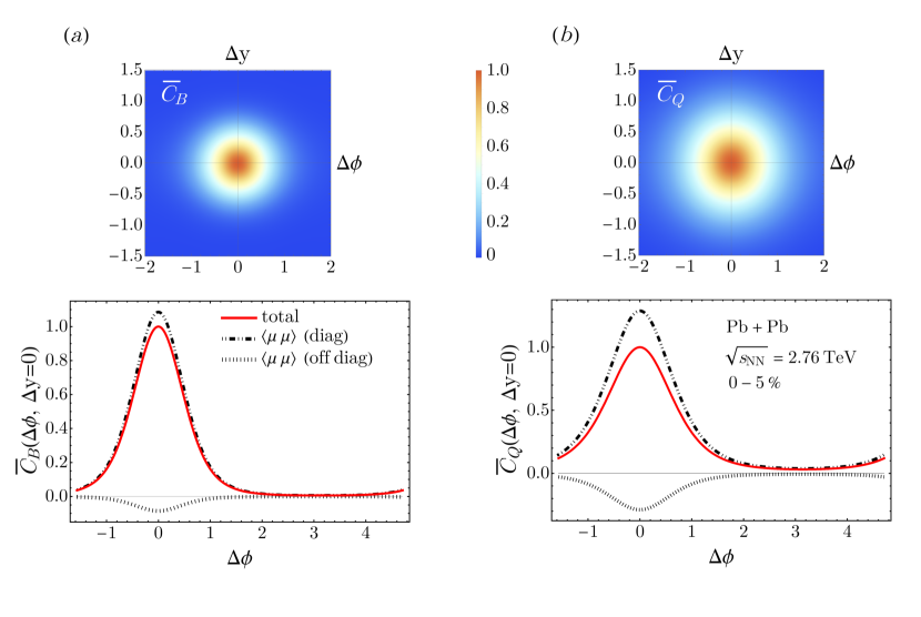
Figure 1: Differential two-particle net-charge correlation, normalized to unity at their peak, as a function of relative azimuthal angle, $\Delta\phi$, and relative momentum rapidity, $\Delta y$. (a): net-baryon correlations, $\bar{C}_{B}$. (b): net-charge correlations, $\bar{C}_{Q}$. The upper panels show two-dimensional profiles, while the lower panels are at fixed $\Delta y=0$. We note that all the contributions from field correlations that are not shown in the graphs, $\langle\chi_{s}\chi_{t}\rangle$, where both $s$ and $t$ do not represent chemical potentials, are zero.

We recall the weighted sum in Eq. (31) defining the two-particle correlation for the net-baryon number:

$$\left\langle E_{p}\frac{dN_{B}}{d^{3}p}E_{q}\frac{dN_{B}}{d^{3}q}\right\rangle=\sum\limits_{jk}B_{j}B_{k}\left\langle E_{p}E_{q}\frac{dN_{jk}}{d^{3}pd^{3}q}\right\rangle.$$ (42)

We compute this quantity from Eq. (III.2) in our framework by considering the contribution of protons and anti-protons, i.e., by taking the common assumption that net-baryon fluctuations correspond to net-proton fluctuations. We integrate Eq. (25) up to $m=10$ and $k=10$, which guarantees convergence, to exhibit the angular dependence of the two-particle correlation,

$$C_{B}(\Delta\phi,\Delta y)\equiv\left\langle E_{p}\frac{dN_{B}}{d^{3}p}E_{q}\frac{dN_{B}}{d^{3}q}\right\rangle(\Delta\phi,\Delta y).$$ (43)

For simplicity we normalize our correlation function in such a way that it is unity at $\Delta\phi=\Delta y=0$,

$$\bar{C}_{B}(\Delta\phi,\Delta y)=C_{B}(\Delta\phi,\Delta y)/C_{B}(0,0).$$ (44)

This allows us to point out generic features of the shape of the correlation function. The normalization can be chosen, then, depending on what is most convenient to measure in experiments. Normalizing the correlation function with the average net baryon charge would lead to a division by very small numbers, especially at ultrarelativistic collision energies. To avoid such issues, one possibility is, for instance, to normalize with standard deviations (which are non-vanishing), and thus construct Pearson correlation coefficients.

Our result for $\bar{C}_{B}$ is displayed in Fig. 1(a). It gives a good illustration of the kind of influence thermal fluctuations have on two-particle correlations.

The correlation is indeed short-range, and leads to a broadening of the near-side peak. The diffusion of the near-side peaks is in fact quite sizable, as the peak drops to half its maximum around the circle $\Delta y=\Delta\phi=1$. We take now a slice of the two-dimension profile corresponding to $\bar{C}_{B}(\Delta\phi,\Delta y=0)$, shown as a red solid line in the bottom panel of Fig. 1(a). Much insight can be gained by decomposing this quantity into contributions coming from different correlators of fluid fields. Since we are looking at a fluctuation of conserved charges that can only be engendered by a fluctuation in the corresponding chemical potentials, we find that the contribution to $\bar{C}_{B}(\Delta\phi,\Delta y=0)$ coming from the variances of the form $\langle\chi_{s}\chi_{t}\rangle$, where both $s$ and $t$ do not represent a chemical potential, is zero. The correlation of the net-baryon number is, thus, produced solely by diagonal and off-diagonal variances of the form $\langle\mu_{B,Q,S}\mu_{B,Q,S}\rangle$. Naturally, in our case of net-proton correlations, the contribution of $\langle\mu_{S}\mu_{S}\rangle$ does vanish, as a fluctuation in $\mu_{S}$ does not change the proton spectrum. The total peak in the bottom panel of Fig. 1(a) gets, thus, a dominant contribution from the diagonal variances $\langle\mu_{B}\mu_{B}\rangle$ and $\langle\mu_{Q}\mu_{Q}\rangle$, and a negative subleading, albeit visible contribution from the off-diagonal one, $\langle\mu_{Q}\mu_{B}\rangle$.

In Fig. 1(b), we perform the same analysis albeit focusing on the net electric charge, $\bar{C}_{Q}(\Delta\phi,\Delta y)$, which we construct from pions, kaons, protons and their antiparticles. The same features are found, though the resulting near-side peak is visibly more diffuse compared to $\bar{C}_{B}$.

We comment now on the implications of this result. One could simply take the particles collected in central Pb+Pb collisions at top Large Hadron Collider energy, and measure the correlation functions depicted in Fig. 1. The question is, hence, to which extent one should expect the experimental result to resemble our theoretical results. While care is needed, there is no obvious reason to believe the experimental results will look entirely different from ours. Within a rapidity window that is large enough to detect all of those decay products, one does not in general expect non-flow phenomena to lead to fluctuations of conserved charges. This may also be investigated by comparing the experimental results to the output of event-generators that include non-flow contributions. Resonance decays may also be added in future to our formalism by modifying the blast-wave parametrization of Eq. (34), as precisely done in Ref. Mazeliauskas:2019ifr . That said, a potential modification of the correlations measured experimentally could however come from self-correlations. Experiments construct their correlation observables from pairs of distinct particles, while this is not something that we require in our calculations. We discuss this subtle point in more depth in Sec. V.3.

V.2 Introducing a finite correlation length

We see that already the use of ultra-local thermal correlations in Eq (38) leads to a significant spread of the near-side peaks in Fig. 1. This suggests that this spread may be effectively independent of whether correlations are local or not. In this subsection, we perform a simple calculation to check this explicitly. We go beyond the ultra-local approximation by replacing the delta functions with exponential decays, characterized, in both $\alpha$, $\varphi$, and $\eta$, by correlation lengths $\xi_{\alpha}$, $\xi_{\varphi}$, $\xi_{\eta}$, respectively, while keeping the same correlation matrix $\sigma_{st}$ as prefactor. Working for convenience with the variables $(\alpha+\alpha^{\prime})/2$ and $\alpha-\alpha^{\prime}$, we have in short:

$$\langle\chi_{s}(x)\chi_{t}(x^{\prime})\rangle =\frac{1}{\sqrt{h(\frac{\alpha+\alpha^{\prime}}{2})}}\sigma_{st}\biggl{(}\frac{\alpha+\alpha^{\prime}}{2}\biggr{)}$$

$$\times\frac{1}{2\xi_{\alpha}}e^{-\tfrac{|\alpha-\alpha^{\prime}|}{\xi_{\alpha}}}\frac{1}{2\xi_{\varphi}}e^{-\tfrac{|\varphi-\varphi^{\prime}|}{\xi_{\varphi}}}\frac{1}{2\xi_{\eta}}e^{-\tfrac{|\eta-\eta^{\prime}|}{\xi_{\eta}}}.$$ (45)

In the calculation of, e.g., $C_{B}(\Delta\phi,\Delta y)$, the part that gets modified is the Fourier coefficient $g_{st}$ in Eq. (41). This requires, once again, to perform Fourier transforms with respect to $\Delta\varphi=\varphi-\varphi^{\prime}$ and $\Delta\eta=\eta-\eta^{\prime}$, i.e.,

$$\int_{-\pi}^{\pi}\frac{d\Delta\varphi}{2\pi}\,\frac{1}{2\xi_{\varphi}}e^{-\tfrac{|\Delta\varphi|}{\xi_{\varphi}}-im\Delta\varphi}\int_{-\infty}^{\infty}d\Delta\eta\frac{1}{2\xi_{\eta}}e^{-\tfrac{|\Delta\eta|}{\xi_{\eta}}-ik\Delta\eta},$$ (46)

which simply yields

$$\begin{split}g_{st}^{(m)}(\alpha,\alpha^{\prime};k)=&\frac{1}{2\pi}\frac{1}{\sqrt{h(\frac{\alpha+\alpha^{\prime}}{2})}}\sigma_{st}\left(\tfrac{\alpha+\alpha^{\prime}}{2}\right)\frac{1}{2\xi_{\alpha}}e^{\tfrac{-|\alpha-\alpha^{\prime}|}{\xi_{\alpha}}}\\ \times&\frac{1}{1+\xi_{\eta}^{2}k^{2}}\frac{1-e^{-\tfrac{\pi}{\xi_{\varphi}}}\cos(m\pi)}{1+\xi_{\varphi}^{2}m^{2}},\end{split}$$ (47)

that depends now on both $m$ and $k$.

For a numerical application, we fix $\xi_{\varphi}=0.01\pi$ and $\xi_{\eta}=0.001$, and we vary $\xi_{\alpha}$. The resulting correlation function, $\bar{C}_{B}(\Delta\phi,\Delta y=0)$, is plotted in Fig. 2. Unsurprisingly, increasing the correlation length along $\alpha$ over a wide interval does yield only a minor additional diffusion of the near-side peak. While this prescription is rather ad hoc, it suggests that the precise shape of the thermal correlators in Eq. (38) may indeed not matter much for the final result. The more crucial ingredient is the thermal correlation matrix.

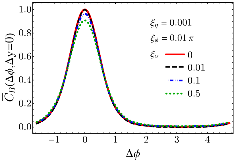
Figure 2: Same as in the lower panel of Fig. 1(a), but with varying correlation length (shown as different line styles) along the $\alpha$ direction, following Eq. (45).

V.3 Self-correlations

Before concluding, let us comment on the issue of self-correlations. Two-particle correlation functions as Eq. (17) can be estimated experimentally in two different ways. The choice is whether the two correlated particles are distinct, or whether the same particle can form a pair with itself. Typically, as done in standard flow analyses, only pairs of distinct particles are chosen, to avoid a strong bias in the resulting correlations. As it stands, the formalism developed in Secs. III and IV.2 features self-correlations. This can be seen in the limit where the thermodynamic equation of state entering the functional $I_{\Sigma[\chi]}$ in (36) is the one for an ideal gas, and non-trivial correlations are in fact of the self-correlation type.

To see this more explicitly, for a non-interacting gas of free streaming particles, one can write at $x^{0}=x^{\prime 0}$ Calzetta:2008iqa

$$\begin{split}&\langle\Delta f_{j}(x,p)\Delta f_{k}(x^{\prime},q)\rangle=\\ &\delta_{jk}(2\pi)^{3}\delta^{(3)}(\mathbf{x}-\mathbf{x}^{\prime})\delta^{(3)}(\mathbf{p}-\mathbf{q})f_{\text{eq}}(x,p)(1\pm f_{\text{eq}}(x,p)),\end{split}$$ (48)

where the upper (lower) sign is for bosons (fermions), or replace $(1\pm f_{\text{eq}})\to 1$ for Boltzmann statistics. One should understand the right-hand side of Eq. (48) as a contribution to the connected pair correlation function in phase space $f_{jk}^{(\text{c})}(x,x^{\prime},p,q)$ in Eq. (7), and, accordingly, it contributes in the freeze-out integral in Eq. (6). This is a contribution from self-correlations. On the other hand, one may take integrals over positions and momenta in Eq. (48) and obtain the second order cumulants of thermodynamic variables, such as energy or conserved particle numbers, as they follow for an ideal (quantum) gas. These arguments show in which sense our formalism reduces to self correlations in the limit of an ideal gas.

Let us stress that existing literature describing hydrodynamic fluctuations in heavy-ion collisions has also been dealing with this question, see e.g. the recent Refs. Kapusta:2017hfi ; De:2020yyx . Fluctuations induced by hydrodynamic noise are evolved in time dynamically, and self-correlations are isolated. Their impact is quantified on measurements on balance functions Pratt:2012dz , and it is indeed a significant correction. In our framework, it might also be possible to subtract self-correlations by modifying the correlation functions on the freeze-out surface. For instance, one could devise an analogue of factorial cumulants Kitazawa:2017ljq , that remove self-correlations by construction. Devising such a subtraction scheme goes beyond the scope of this work, such that our framework has self-correlations included. Future experimental measurements of the quantities proposed in Fig. 1 should probably be performed both with and without self-correlations, to assess their effect.

VI Conclusion and outlook

In this manuscript we have addressed a rather straightforward problem. Given a surface $\Sigma$ characterized by a set of fluid fields, we have studied position-space correlations among such fields induced by thermal fluctuations on $\Sigma$. Identifying $\Sigma$ with the kinetic freeze-out surface of heavy-ion collisions, we have then translated such correlations into momentum-space correlations at the particlization of such surface following the Cooper-Frye formula generalized to account for genuine two-body contributions. A straightforward application of our formulas combining a blast-wave parametrization of the average momentum yields with the thermal correlation functions of an ideal resonance gas leads to the emergence of angular net-charge correlations from thermal fluctuations at the freeze-out surface. An interesting diffusion of the near-side peak is observed, which we expect may motivate further experimental and theoretical developments.

Experimentally, the proposed non-flow correlations can be measured straightforwardly. The long-range contribution from the hydrodynamic flow can be removed from the near-side peak by fitting its shape at the away-side peak. For the correlatons of net charges, it would be interesting, in particular, to compare experimental data with the output of traditional event generators, which do not include potential effects of dynamical fluctuations. This can be done both at top LHC energy where $\mu_{B,Q,S}=0$, as well as a function of beam energy at RHIC, where our results could be generalized to include finite chemical potentials (albeit with a background freeze-out surface that is no longer boost-invariant).

On the theory side, our calculations can certainly be improved in several ways, by, e.g., adding viscous corrections at freeze-out, relaxing the strong equilibrium hypothesis, as well as implementing an equation of state allowing for a more sensible study of critical phenomena. The issue of self-correlation may also be addressed in future, possibly, by devising optimal correlation functions to eliminate them, much as done in Ref. De:2020yyx .

We deem that calculations of angular and longitudinal correlations of net-charges will represent remarkable results in themselves, whose comparison with experimental data will open a new window onto the nontrivial thermal fluctuation properties of the quark-gluon plasma.

VII Acknowledgments

We thank the members of the C06 project “Flow and fluctuations in relativistic heavy-ion collisions” within the ISOQUANT Collaborative Research Centre for useful discussion related to the topic of this work. We acknowledge useful discussions with Eduardo Grossi. This work is supported by the Deutsche Forschungsgemeinschaft (DFG, German Research Foundation) under Germany’s Excellence Strategy EXC 2181/1 - 390900948 (the Heidelberg STRUCTURES Excellence Cluster) and under 273811115 – SFB 1225 ISOQUANT as well as FL 736/3-1. This work is partially financed by the Baden-Württemberg Stiftung gGmbH.

Appendix A Thermal correlation functions of an ideal gas

We exhibit in this appendix the full derivation of the correlator $\langle\chi_{n}(\alpha)\chi_{m}(\alpha^{\prime})\rangle_{c}$ in Eq. (38), i.e.,

$$\langle\chi_{s}(\alpha)\chi_{t}(\alpha^{\prime})\rangle_{c}=\frac{1}{\sqrt{h(\alpha)}}\delta^{(3)}(\alpha-\alpha^{\prime})\sigma_{st}(\alpha),$$ (49)

where we derive as well the thermal correlation matrix, $\sigma_{st}$.

A.1 Generating functionals for statistical fluctuations on the freeze-out surface

Let us consider a three-dimensional hypersurface $\Sigma$ of four-dimensional space-time. We want to characterize statistical (e. g. thermal) fluctuations thereon. We assume that the hypersurface is parametrized by a coordinate system $\alpha^{j}$ with $j=1,2,3$. The embedding into space-time is given by the map $x^{\mu}(\alpha)$. The induced metric in the three-dimensional space is

$$h_{jk}(\alpha)=g_{\mu\nu}\left[\frac{\partial}{\partial\alpha^{j}}x^{\mu}(\alpha)\right]\left[\frac{\partial}{\partial\alpha^{k}}x^{\nu}(\alpha)\right],$$ (50)

where $g_{\mu\nu}={\rm diag}(-,+,+,+)_{\mu\nu}$. We consider now that, for a given field configuration $\chi$, the probability density of fluctuations on the freeze-out surface, $\Sigma$, can be written as a functional

$$p[\chi]=\frac{1}{Z_{\Sigma}}e^{-I_{\Sigma}[\chi]},$$ (51)

with partition function

$$Z_{\Sigma}=\int D\chi\;e^{-I_{\Sigma}[\chi]}.$$ (52)

In the last equation we have introduced the functional integral $\int D\chi=\int D\chi_{1}\cdots\int D\chi_{n}$ on the surface $\Sigma$. The partition function on the freeze-out surface can be generalized to include external sources, $J_{n}$,

$$Z_{\Sigma}[J]=\int D\chi\;\exp\left[-I_{\Sigma}[\chi]+\int d^{3}\alpha\sqrt{h}J_{n}(\alpha)\chi(\alpha)\right],$$ (53)

with $\sqrt{h}=\sqrt{\text{det}(h_{jk})}$ and the invariant hypersurface element $d^{3}\alpha\sqrt{h}$. Correlation functions are then obtained as functional derivatives of the partition function, e. g.

$$\begin{split}&\langle\chi_{n}(\alpha)\chi_{m}(\beta)\rangle=\\ &\frac{1}{Z_{\Sigma}[J]}\left(\frac{1}{\sqrt{h(\alpha)}}\frac{\delta}{\delta J_{n}(\alpha)}\right)\left(\frac{1}{\sqrt{h(\beta)}}\frac{\delta}{\delta J_{m}(\beta)}\right)Z_{\Sigma}[J]{\big{|}}_{J=0}.\end{split}$$ (54)

One may also introduce the generating functional for the connected correlation functions $W_{\Sigma}[J]=\ln Z_{\Sigma}[J]$ such that e. g.

$$\begin{split}&\langle\chi_{n}(\alpha)\chi_{m}(\beta)\rangle_{c}=\langle\chi_{n}(\alpha)\chi_{m}(\beta)\rangle-\langle\chi_{n}(\alpha)\rangle\langle\chi_{m}(\beta)\rangle\\ &=\left(\frac{1}{\sqrt{h(\alpha)}}\frac{\delta}{\delta J_{n}(\alpha)}\right)\left(\frac{1}{\sqrt{h(\beta)}}\frac{\delta}{\delta J_{m}(\beta)}\right)W[J]{\big{|}}_{J=0}.\end{split}$$ (55)

All the relevant information about connected correlations on the freeze-out surface is encoded in $W_{\Sigma}[J]$. Determining this functional is of course a very nontrivial problem, already in, or close-to, thermal equilibrium for a strongly interacting theory like QCD. For vanishing baryon number chemical potential, one can in principle hope to obtain $W_{\Sigma}[J]$ from lattice QCD calculations. However, the determination of such local correlation functions would require prohibitive “numerical statistics” compared to the determination of global correlations, such as for integrated particle numbers or charges in some volume.

A.2 Local equilibrium approximation to correlation functions

To make progress, we assume thermal equilibrium in small fluid cells. The probability for $\chi$ is then determined by a change in entropy Landau:1980mil

$$p[\chi]=\text{const}\times e^{\Delta S[\chi]},$$ (56)

which can be directly related to eq. (51),

$$I_{\Sigma}[\chi]=-\Delta S[\chi]+\text{const}~{}.$$ (57)

The additive constant is in fact irrelevant because it drops out in a calculation of correlation functions. For fluctuations of conserved quantities such as the four-momentum, $P^{\mu}$, and particle number, $N_{j}$, one can write locally

$$dS=\beta_{\nu}dP^{\nu}+\sum_{j}\alpha_{j}dN_{j},$$ (58)

with $\beta_{\nu}=u_{\nu}/T$, $T$ being the temperature, and $\alpha_{j}=\mu_{j}/T$ is the ratio of chemical potential, $\mu_{j}$, conjugate to the particle number $N_{j}$ and temperature $T$.

We split now the system into two parts - a subsystem labeled by an index $1$, and a bath labeled by $0$. We consider, then, that the change in entropy splits additively, $dS=dS_{0}+dS_{1}$, such that

$$\begin{split}dS=&dS_{0}+dS_{1}\\ =&\beta_{0,\nu}dP_{0}^{\nu}+\beta_{1,\nu}dP_{1}^{\nu}+\sum_{j}\alpha_{j,0}dN_{j,0}+\sum_{j}\alpha_{j,1}dN_{j,1},\\ =&\Delta\beta_{\nu}dP^{\nu}+\sum_{j}\Delta\alpha_{j}dN_{j}\end{split}$$ (59)

where, to obtain the last line, we have used the conservation laws $dP_{0}^{\nu}+dP_{1}^{\nu}=0$ and $dN_{j,0}+dN_{j,1}=0$, and set $\Delta\beta_{\nu}=\beta_{\nu,1}-\beta_{\nu,0}$ and $\Delta\alpha_{j}=\alpha_{j,1}-\alpha_{j,0}$. We also abbreviate $dP^{\nu}=dP^{\nu}_{1}$ and $dN_{j}=dN_{j,1}$. Now, we denote by $\Delta P^{\nu}$ and $\Delta N_{j}$ the amount of conserved quantities that are (temporarily) transmitted from the bath to the subsystem, while $\Delta\beta_{\nu}$ and $\Delta\alpha_{j}$ denote associated differences in conjugate fields. The latter are not independent of the former, but one can assume that $\Delta\beta_{\nu}$ and $\Delta\alpha_{j}$ are linear in $\Delta P^{\nu}$ and $\Delta N_{j}$, to lowest order in the variations. With this consideration, integration of Eq. (59) leads to

$$\Delta S=\frac{1}{2}\left(\Delta\beta_{\nu}\Delta P^{\nu}+\sum_{j}\Delta\alpha_{j}\Delta N_{j}\right).$$ (60)

In the next step, we assume that the above considerations hold for every small volume $d^{3}\alpha\sqrt{h}$ of the hypersurface $\Sigma$. This is a strong form of local equilibrium hypothesis, assuming that different volume elements are independent and that all correlation functions are short range. Keeping this in mind, from Eq. (57) we obtain

$$I_{\Sigma}=-\Delta S=\frac{1}{2}\int d\Sigma_{\mu}\left\{\Delta\beta_{\nu}\Delta T^{\mu\nu}+\sum_{j}\Delta\alpha_{j}\Delta N_{j}^{\mu}\right\},$$ (61)

where we have employed the surface element $d\Sigma_{\mu}=d^{3}\alpha\sqrt{h}n_{\mu}$ with future pointing normal vector $n_{\mu}$ and we have used that locally $\Delta P^{\nu}=-\int d\Sigma_{\mu}\Delta T^{\mu\nu}$ with energy-momentum tensor $T^{\mu\nu}$ and similarly $\Delta N_{j}=-\int d\Sigma_{\mu}\Delta N_{j}^{\mu}$ with number current $N_{j}^{\mu}$ (the minus signs are again due to the metric signature $(-,+,+,+)$).

The variation of the energy-momentum tensor, $\Delta T^{\mu\nu}$, and of the particle number current, $\Delta N^{\mu}$, can now be derived from their expression in the ideal fluid case considered throughout this manuscript

$$T^{\mu\nu}=\epsilon u^{\mu}u^{\nu}+p\Delta^{\mu\nu},\quad\quad\quad N_{j}^{\mu}=n_{j}u^{\mu}.$$ (62)

We choose as independent fields the three independent components of fluid velocity, $u^{\mu}$, the temperature, $T$, and the chemical potentials, $\mu_{j}$, and we consider that to linear order in $\Delta u^{\mu}$ one has $u_{\mu}\Delta u^{\mu}=0$. The linear variation in the energy momentum tensor is, consequently, given by

$$\begin{split}&\Delta T^{\mu\nu}=\left[\left(T\tfrac{\partial^{2}p}{\partial T^{2}}+\sum\limits_{i}\mu_{i}\tfrac{\partial^{2}p}{\partial T\partial\mu_{i}}\right)u^{\mu}u^{\nu}+\tfrac{\partial p}{\partial T}\Delta^{\mu\nu}\right]\Delta T\\ &+\sum\limits_{i}\left[\left(\sum_{j}\mu_{j}\tfrac{\partial^{2}p}{\partial\mu_{i}\partial\mu_{j}}+T\tfrac{\partial^{2}p}{\partial T\partial\mu_{i}}\right)u^{\mu}u^{\nu}+\tfrac{\partial p}{\partial\mu_{i}}\Delta^{\mu\nu}\right]\Delta\mu_{i}\\ &+\left[\left(T\tfrac{\partial p}{\partial T}+\sum_{i}\mu_{i}\tfrac{\partial p}{\partial\mu_{i}}\right)\left(\delta_{\rho}^{\mu}u^{\nu}+u^{\mu}\delta_{\rho}^{\nu}\right)\right]\Delta u^{\rho},\end{split}$$ (63)

while for the conserved particle currents

$$\begin{split}\Delta N^{\mu}_{i}=&\left[\tfrac{\partial^{2}p}{\partial T\partial\mu_{i}}u^{\mu}\right]\Delta T+\sum\limits_{j}\left[\tfrac{\partial^{2}p}{\partial\mu_{i}\partial\mu_{j}}u^{\mu}\right]\Delta\mu_{j}\\ &+\left[\tfrac{\partial p}{\partial\mu_{i}}\delta_{\rho}^{\mu}\right]\Delta u^{\rho}.\end{split}$$ (64)

Inserting these expression in Eq. (61) leads to a quadratic functional of the fluctuation fields

$$\begin{split}I_{\Sigma}=\frac{1}{2}\int d\Sigma_{\mu}{\Bigg{\{}}&\frac{u^{\mu}}{T}{\bigg{(}}\tfrac{\partial^{2}p}{\partial T^{2}}\Delta T^{2}+2\sum\limits_{j}\tfrac{\partial^{2}p}{\partial T\partial\mu_{j}}\Delta T\Delta\mu_{j}\\ &+\sum\limits_{i,j}\tfrac{\partial^{2}p}{\partial\mu_{i}\partial\mu_{j}}\Delta\mu_{i}\Delta\mu_{j}{\bigg{)}}\\ &+2\frac{\Delta u^{\mu}}{T}{\bigg{(}}\tfrac{\partial p}{\partial T}\Delta T+\sum_{j}\tfrac{\partial p}{\partial\mu_{j}}\Delta\mu_{j}{\bigg{)}}\\ &+\frac{u^{\mu}}{T}\left(\epsilon+p\right)\Delta_{\rho\sigma}\Delta u^{\rho}\Delta u^{\sigma}{\Bigg{\}}}.\end{split}$$ (65)

We note that Eq. (65), when used in Eq. (51), defines a Gaussian probability distribution for the fields $\Delta T$, $\Delta\mu_{j}$ and the three independent components of $\Delta u^{\mu}$. We also note that the probability functional is ultra-local in the sense that it contains no spatial derivatives of the thermodynamic fields. To relax this assumption, one would have to go beyond the strong local equilibrium assumption, resorting for example to a derivative expansion.

A.3 Thermal correlation matrix

Being Gaussian, the functional integral defining the partition function in Eq. (53) can easily be performed. Up to an irrelevant constant, one finds

$$Z_{\Sigma}[J]=\exp\left[\frac{1}{2}\int d^{3}\alpha\sqrt{h}J_{n}(\alpha)\sigma_{nm}(\alpha)J_{m}(\alpha)\right],$$ (66)

where $\sigma_{nm}(\alpha)$ is a matrix of local variances such that

$$\langle\chi_{n}(\alpha)\chi_{m}(\alpha^{\prime})\rangle_{c}=\frac{1}{\sqrt{h(\alpha)}}\delta^{(3)}(\alpha-\alpha^{\prime})\sigma_{nm}(\alpha).$$ (67)

One can in fact directly read of the inverse of $\sigma_{nm}$ from equation (65) by writing

$$I_{\Sigma}[\chi]=\frac{1}{2}\int d^{3}\alpha\sqrt{h}\,\chi_{n}(\alpha)(\sigma^{-1})_{nm}\chi_{m}(\alpha).$$ (68)

Choosing as variables $\chi_{n}=(\Delta T,\Delta\mu_{i},\Delta u^{\rho})$ and taking into account that $d\Sigma_{\mu}=d^{3}\alpha\sqrt{h}\,n_{\mu}$ with normal vector $n_{\mu}$ leads to

$$\sigma^{-1}=\begin{pmatrix}-\frac{n\cdot u}{T}\frac{\partial^{2}p}{\partial T^{2}}&-\frac{n\cdot u}{T}\frac{\partial^{2}p}{\partial T\partial\mu_{j}}&-\frac{n_{\sigma}}{T}\frac{\partial p}{\partial T}\\ -\frac{n\cdot u}{T}\frac{\partial^{2}p}{\partial T\partial\mu_{i}}&-\frac{n\cdot u}{T}\frac{\partial^{2}p}{\partial\mu_{i}\partial\mu_{j}}&-\frac{n_{\sigma}}{T}\frac{\partial p}{\partial\mu_{j}}\\ -\frac{n_{\rho}}{T}\frac{\partial p}{\partial T}&-\frac{n_{\rho}}{T}\frac{\partial p}{\partial\mu_{i}}&-\frac{n\cdot u}{T}(\epsilon+p)\Delta_{\rho\sigma}\end{pmatrix}.$$ (69)

This matrix can easily be inverted in a concrete application. Note that its entries are determined by the equation of state of the considered system.

References

- (1) P. Braun-Munzinger and J. Stachel, Nature 448, 302-309 (2007) doi:10.1038/nature06080
- (2) W. Busza, K. Rajagopal and W. van der Schee, Ann. Rev. Nucl. Part. Sci. 68, 339-376 (2018) doi:10.1146/annurev-nucl-101917-020852 [arXiv:1802.04801 [hep-ph]].
- (3) P. Romatschke and U. Romatschke, doi:10.1017/9781108651998 [arXiv:1712.05815 [nucl-th]].
- (4) S. Schlichting and D. Teaney, Ann. Rev. Nucl. Part. Sci. 69, 447-476 (2019) doi:10.1146/annurev-nucl-101918-023825 [arXiv:1908.02113 [nucl-th]].
- (5) J. Berges, M. P. Heller, A. Mazeliauskas and R. Venugopalan, Rev. Mod. Phys. 93, no.3, 035003 (2021) doi:10.1103/RevModPhys.93.035003 [arXiv:2005.12299 [hep-th]].
- (6) M. Luzum and H. Petersen, J. Phys. G 41, 063102 (2014) doi:10.1088/0954-3899/41/6/063102 [arXiv:1312.5503 [nucl-th]].
- (7) M. Cheng, P. Hegde, C. Jung, F. Karsch, O. Kaczmarek, E. Laermann, R. D. Mawhinney, C. Miao, P. Petreczky and C. Schmidt, et al. Phys. Rev. D 79, 074505 (2009) doi:10.1103/PhysRevD.79.074505 [arXiv:0811.1006 [hep-lat]].
- (8) K. Fukushima and T. Hatsuda, Rept. Prog. Phys. 74, 014001 (2011) doi:10.1088/0034-4885/74/1/014001 [arXiv:1005.4814 [hep-ph]].
- (9) A. Bzdak, S. Esumi, V. Koch, J. Liao, M. Stephanov and N. Xu, Phys. Rept. 853, 1-87 (2020) doi:10.1016/j.physrep.2020.01.005 [arXiv:1906.00936 [nucl-th]].
- (10) M. Bluhm, A. Kalweit, M. Nahrgang, M. Arslandok, P. Braun-Munzinger, S. Floerchinger, E. S. Fraga, M. Gazdzicki, C. Hartnack and C. Herold, et al. Nucl. Phys. A 1003, 122016 (2020) doi:10.1016/j.nuclphysa.2020.122016 [arXiv:2001.08831 [nucl-th]].
- (11) J. I. Kapusta, B. Muller and M. Stephanov, Phys. Rev. C 85, 054906 (2012) doi:10.1103/PhysRevC.85.054906 [arXiv:1112.6405 [nucl-th]].
- (12) C. Young, Phys. Rev. C 89, no.2, 024913 (2014) doi:10.1103/PhysRevC.89.024913 [arXiv:1306.0472 [nucl-th]].
- (13) B. Ling, T. Springer and M. Stephanov, Phys. Rev. C 89, no.6, 064901 (2014) doi:10.1103/PhysRevC.89.064901 [arXiv:1310.6036 [nucl-th]].
- (14) C. Young, J. I. Kapusta, C. Gale, S. Jeon and B. Schenke, Phys. Rev. C 91, no.4, 044901 (2015) doi:10.1103/PhysRevC.91.044901 [arXiv:1407.1077 [nucl-th]].
- (15) K. Murase, doi:10.15083/00072981
- (16) L. Yan and H. Grönqvist, JHEP 03, 121 (2016) doi:10.1007/JHEP03(2016)121 [arXiv:1511.07198 [nucl-th]].
- (17) K. Nagai, R. Kurita, K. Murase and T. Hirano, Nucl. Phys. A 956, 781-784 (2016) doi:10.1016/j.nuclphysa.2016.02.007 [arXiv:1602.00794 [nucl-th]].
- (18) S. Gavin, G. Moschelli and C. Zin, Phys. Rev. C 94, no.2, 024921 (2016) doi:10.1103/PhysRevC.94.024921 [arXiv:1606.02692 [nucl-th]].
- (19) Y. Akamatsu, A. Mazeliauskas and D. Teaney, Phys. Rev. C 95, no.1, 014909 (2017) doi:10.1103/PhysRevC.95.014909 [arXiv:1606.07742 [nucl-th]].
- (20) A. Sakai, K. Murase and T. Hirano, Nucl. Phys. A 967, 445-448 (2017) doi:10.1016/j.nuclphysa.2017.05.010
- (21) J. I. Kapusta and C. Plumberg, Phys. Rev. C 97, no.1, 014906 (2018) [erratum: Phys. Rev. C 102, no.1, 019901 (2020)] doi:10.1103/PhysRevC.97.014906 [arXiv:1710.03329 [nucl-th]].
- (22) C. Chattopadhyay, R. S. Bhalerao and S. Pal, Phys. Rev. C 97, no.5, 054902 (2018) doi:10.1103/PhysRevC.97.054902 [arXiv:1711.10759 [nucl-th]].
- (23) M. Stephanov and Y. Yin, Phys. Rev. D 98, no.3, 036006 (2018) doi:10.1103/PhysRevD.98.036006 [arXiv:1712.10305 [nucl-th]].
- (24) M. Singh, C. Shen, S. McDonald, S. Jeon and C. Gale, Nucl. Phys. A 982, 319-322 (2019) doi:10.1016/j.nuclphysa.2018.10.061 [arXiv:1807.05451 [nucl-th]].
- (25) Y. Akamatsu, D. Teaney, F. Yan and Y. Yin, Phys. Rev. C 100, no.4, 044901 (2019) doi:10.1103/PhysRevC.100.044901 [arXiv:1811.05081 [nucl-th]].
- (26) X. An, G. Basar, M. Stephanov and H. U. Yee, Phys. Rev. C 100, no.2, 024910 (2019) doi:10.1103/PhysRevC.100.024910 [arXiv:1902.09517 [hep-th]].
- (27) K. Murase, Annals Phys. 411, 167969 (2019) doi:10.1016/j.aop.2019.167969 [arXiv:1904.11217 [nucl-th]].
- (28) X. An, G. Başar, M. Stephanov and H. U. Yee, Phys. Rev. C 102, no.3, 034901 (2020) doi:10.1103/PhysRevC.102.034901 [arXiv:1912.13456 [hep-th]].
- (29) A. De, C. Plumberg and J. I. Kapusta, Phys. Rev. C 102, no.2, 024905 (2020) doi:10.1103/PhysRevC.102.024905 [arXiv:2003.04878 [nucl-th]].
- (30) A. Sakai, K. Murase and T. Hirano, Phys. Rev. C 102, no.6, 064903 (2020) doi:10.1103/PhysRevC.102.064903 [arXiv:2003.13496 [nucl-th]].
- (31) J. Chao and T. Schaefer, JHEP 01, 071 (2021) doi:10.1007/JHEP01(2021)071 [arXiv:2008.01269 [hep-th]].
- (32) A. Sakai, K. Murase and T. Hirano, [arXiv:2111.08963 [nucl-th]].
- (33) F. Cooper and G. Frye, Phys. Rev. D 10, 186 (1974) doi:10.1103/PhysRevD.10.186
- (34) D. Teaney, Phys. Rev. C 68, 034913 (2003) doi:10.1103/PhysRevC.68.034913 [arXiv:nucl-th/0301099 [nucl-th]].
- (35) J. F. Paquet, C. Shen, G. S. Denicol, M. Luzum, B. Schenke, S. Jeon and C. Gale, Phys. Rev. C 93, no.4, 044906 (2016) doi:10.1103/PhysRevC.93.044906 [arXiv:1509.06738 [hep-ph]].
- (36) E. A. Calzetta and B. L. B. Hu, doi:10.1017/CBO9780511535123
- (37) J. D. Bjorken, Phys. Rev. D 27, 140-151 (1983) doi:10.1103/PhysRevD.27.140
- (38) M. Luzum, J. Phys. G 38, 124026 (2011) doi:10.1088/0954-3899/38/12/124026 [arXiv:1107.0592 [nucl-th]].
- (39) M. A. Stephanov, K. Rajagopal and E. V. Shuryak, Phys. Rev. Lett. 81, 4816-4819 (1998) doi:10.1103/PhysRevLett.81.4816 [arXiv:hep-ph/9806219 [hep-ph]].
- (40) C. Schwarz, D. Oliinychenko, L. G. Pang, S. Ryu and H. Petersen, J. Phys. G 45, no.1, 015001 (2018) doi:10.1088/1361-6471/aa90eb [arXiv:1707.07026 [hep-ph]].
- (41) D. Oliinychenko and V. Koch, Phys. Rev. Lett. 123, no.18, 182302 (2019) doi:10.1103/PhysRevLett.123.182302 [arXiv:1902.09775 [hep-ph]].
- (42) D. Oliinychenko, S. Shi and V. Koch, Phys. Rev. C 102, no.3, 034904 (2020) doi:10.1103/PhysRevC.102.034904 [arXiv:2001.08176 [hep-ph]].
- (43) V. Vovchenko, [arXiv:2106.13775 [hep-ph]].
- (44) E. Schnedermann, J. Sollfrank and U. W. Heinz, Phys. Rev. C 48, 2462-2475 (1993) doi:10.1103/PhysRevC.48.2462 [arXiv:nucl-th/9307020 [nucl-th]].
- (45) V. Vovchenko, D. V. Anchishkin and M. I. Gorenstein, Phys. Rev. C 91, no.2, 024905 (2015) doi:10.1103/PhysRevC.91.024905 [arXiv:1412.5478 [nucl-th]].
- (46) A. Mazeliauskas and V. Vislavicius, Phys. Rev. C 101, no.1, 014910 (2020) doi:10.1103/PhysRevC.101.014910 [arXiv:1907.11059 [hep-ph]].
- (47) P. A. Zyla et al. [Particle Data Group], PTEP 2020, no.8, 083C01 (2020) doi:10.1093/ptep/ptaa104
- (48) S. Pratt, Phys. Rev. Lett. 108, 212301 (2012) doi:10.1103/PhysRevLett.108.212301 [arXiv:1203.4578 [nucl-th]].
- (49) M. Kitazawa and X. Luo, Phys. Rev. C 96, no.2, 024910 (2017) doi:10.1103/PhysRevC.96.024910 [arXiv:1704.04909 [nucl-th]].
- (50) L. D. Landau and E. M. Lifshitz, “Statistical Physics, Part 1,” ISBN: 9780750633727, Butterworth-Heinemann, Oxford, 1980
- (51) S. Floerchinger and T. Haas, Phys. Rev. E 102, no.5, 052117 (2020) doi:10.1103/PhysRevE.102.052117 [arXiv:2004.13533 [cond-mat.stat-mech]].