3D Tomographic Phase Retrieval and Unwrapping

Abstract.

This paper develops uniqueness theory for 3D phase retrieval with finite, discrete measurement data for strong phase objects and weak phase objects, including:

(i) Unique determination of (phase) projections from diffraction patterns – General measurement schemes with coded and uncoded apertures are proposed and shown to ensure unique reduction of diffraction patterns to the phase projection for a strong phase object (respectively, the projection for a weak phase object) in each direction separately without the knowledge of relative orientations and locations. (ii) Uniqueness for 3D phase unwrapping – General conditions for unique determination of a 3D strong phase object from its phase projection data are established, including, but not limited to, random tilt schemes densely sampled from a spherical triangle of vertexes in three orthogonal directions and other deterministic tilt schemes. (iii) Uniqueness for projection tomography – Unique determination of an object of $n^{3}$ voxels from generic $n$ projections or $n+1$ coded diffraction patterns is proved.

This approach of reducing 3D phase retrieval to the problem of (phase) projection tomography has the practical implication of enabling classification and alignment, when relative orientations are unknown, to be carried out in terms of (phase) projections, instead of diffraction patterns.

The applications with the measurement schemes such as single-axis tilt, conical tilt, dual-axis tilt, random conical tilt and general random tilt are discussed.

1. Introduction

Diffraction is crucial in structure determination via high-resolution X-ray and electron microscopies due to the high sensitivity of the phase contrast mechanism [46, 5, 37, 91]. Compared to real-space imaging with lenses, like that in transmission electron microscopy, lensless diffraction methods are aberration-free and have the potential to deliver equivalent resolution using fewer photons/electrons [49, 19].

Although single crystal X-ray diffraction is the most commonly used technique for 3D structure determination, the limited crystallinity of many materials often makes obtaining sufficiently large and well-ordered crystals for X-ray diffraction challenging [47]. This obstacle has inspired the development of coherent diffractive imaging for non-periodic structures.

X-ray and electron diffractions for non-periodic objects can be realized in two imaging modalities: diffraction tomography and single-particle imaging/reconstruction (Figure 1). The former involves a sizable object capable of enduring illuminations from various directions, while the latter handles multiple copies of a particle, such as a biomolecule, in different orientations [11, 92, 73, 12, 56, 3]. These two modalities are mathematically equivalent, except that in single-particle reconstruction, the uncertainty levels vary concerning the relative orientations and locations between the object and the measurement set-up and depend on the sample delivery methods [13, 98, 52, 20, 75, 86].

Since the wavelengths of X-ray and electron waves are extremely short, only intensity measurement data can be collected. To emphasize this aspect we refer to the two imaging modalities as 3D phase retrieval.

Phase retrieval is the process of estimating the phase of a wave from intensity measurements because phase information cannot be directly measured in most imaging systems. In contrast, phase unwrapping is necessary when the phase of a wave is already known but is ’wrapped’ due to its cyclical nature. The phase of a wave, typically measured modulo $2\pi$, repeats every $2\pi$ with values recorded between $-\pi$ and $\pi$, or between 0 and $2\pi$. When the actual phase exceeds this range, it ’wraps’ around, creating ambiguities in the phase data. Phase unwrapping resolves these ambiguities to recover the true phase map.

Our goal is to develop a theory of uniqueness for 3D phase retrieval with finite, discrete measurement data for both strong phase and weak phase objects. To accomplish this, we propose pairwise diffraction measurement schemes and analyze the conditions necessary for the unique determination of the phase projection for a strong phase object, and the projection for a weak phase object in each direction. For a strong phase object, the provided phase projection data contain only the wrapped phase information, so we propose a framework and tilt schemes to address the resulting 3D phase unwrapping problem. For a weak phase object, we analyze the resulting problem of projection tomography and derive explicit conditions for the unique determination of the object of $n^{3}$ voxels from $n$ projection data or $n+1$ coded diffraction patterns.

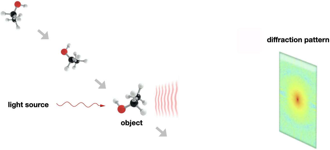
Figure 1. Serial crystallography: A stream of identical particles in various orientations scatter the incident wave with diffraction patterns measured in far field.

1.1. Forward model

Let $n(\mathbf{r})\in\mathbb{C}$ denote the complex refractive index at the point $\mathbf{r}\in\mathbb{R}^{3}$. The real and imaginary components of $n(\mathbf{r})$ describe the dispersive and absorptive aspects of the wave-matter interaction. The real part is related to electron density in the case of X-rays and Coulomb field in the case of electron waves.

Suppose that $z$ is the optical axis in which the incident plane wave $e^{{\rm i}\kappa z}$ propagates. For a quasi-monochromatic wave field $u$ such as coherent X-rays and electron waves, it is useful to write $u=e^{{\rm i}\kappa z}v$ to factor out the incident wave and focus on the modulation field (i.e. the envelope), described by $v$.

The modulation field $v$ satisfies the paraxial wave equation [76]

(1) $${\rm i}\kappa{\partial\over\partial z}v+{1\over 2}\Delta_{\perp}v+\kappa^{2}fv=0,\quad f:=(n^{2}-1)/2$$

where $\Delta_{\perp}=\nabla_{\perp}^{2},\nabla_{\perp}=(\partial_{x},\partial_{y})$, derived from the fundamental wave equation by the so called small-angle approximation (hence the term “paraxial wave”) which requires the wavelength $\lambda$ to be smaller than the maximal distance $d$ over which the fractional variation of $f$ is negligible [53].

In view of different scaling regimes involved in the set-up (Figure 1 and 2), we now break up the forward model into two components: First, a large Fresnel number regime from the entrance pupil to the exit plane; Second, a small Fresnel number regime from the exit plane to the detector plane.

For the exit wave, consider the large Fresnel number regime

(2) $$N_{\rm F}={d^{2}\over\lambda\ell}\gg 1$$

where $\ell$ is the linear size of the object. By rescaling the coordinates

$$z\longrightarrow\ell z,\quad(x,y)\longrightarrow d(x,y)$$

we non-dimensionalize (1) as

$${\rm i}{\partial\over\partial z}v+{1\over 4\pi}N^{-1}_{\rm F}\Delta_{\perp}v+\kappa\ell fv=0,$$

which has a diminishing diffraction term $\Delta_{\perp}$ under (2).

After dropping the $\Delta_{\perp}$ term, the reduced equation in terms of the original coordinates before rescaling is

$${\rm i}{\partial\over\partial z}v+\kappa fv=0,$$

which can be solved by integrating along the optical axis as

(3) $$v(\mathbf{r}) = e^{{\rm i}\kappa\psi(\mathbf{r})},$$

(4) $$\psi(x,y,z) = \int_{-\infty}^{z}f(x,y,z^{\prime})dz^{\prime}.$$

Alternatively, (3)-(4) can be derived by stationary phase analysis [53] or the high-frequency Rytov approximation [71].

The exit wave is given by $u=e^{{\rm i}\kappa z}v$ evaluated at the object’s rear boundary (say, $z=0$). At $z=+\infty$, (4) is called the ray transform, or simply the projection, of the object $f$ in the $z$ direction and (3) will be called the phase projection which equals the exit wave, up to a constant phase factor [72].

By allowing significant phase fluctuations with arbitrary $\kappa|\psi|$, (3)-(4) is an improvement over the weak-phase-object approximation

(5) $$e^{{\rm i}\kappa\psi} \approx 1+{\rm i}\kappa\psi$$

often used in cryo-electron microscopy (cryo-EM) [34, 41, 1]. Following the nomenclature in [41] and [89], we call (3)-(4) the strong-phase-object approximation, noting, however, that $f$ is a complex-valued function in general (thus $e^{{\rm i}\kappa\psi}$ not a “phase” object per se). The strong-phase-object approximation is often invoked the high-frequency forward scattering problems such as diffraction tomography and X-ray diffractive imaging (see, e.g. [36, 23, 42, 43, 93]). In view of (5), the weak-phase-object approximation is the first order Born approximation of the strong-phase-object approximation. The applicability and accuracy of the Born and Rytov approximations has been well studied [57, 80, 96, 14, 58].

However, the exit wave described by the phase projection (3) yields only the information of the projection of $f$ modulo $2\pi/\kappa$, and therein arises the problem of phase unwrapping, which is fundamentally unsolvable unless additional prior information is known (see Section 4) and poses a major road block to the implementation of diffraction tomography. The solution for phase unwrapping is critical in revealing the depth dimension of the object. In contrast, phase unwrapping problem is not present in computed tomography [71], which neglects diffraction, or , cryo-EM which operates under the weak-phase-object approximation (5).

Between the strong- and weak-phase-object approximations, there is a family of hybrid approximations which take the form

(6) $$v_{q}=\Big{(}1+{{\rm i}\kappa\psi\over q}\Big{)}^{q},\quad q\in\mathbb{R},$$

[65, 67]. Clearly, the weak-phase-object approximation corresponds to $q=1$ while $v_{q}$ tends to the phase projection (3) as $q\to\infty.$ In the hybrid approximation, the complex phase $\psi$ is given by

$$\psi_{q}={q\over{\rm i}\kappa}\left(v_{q}^{1/q}-1\right)$$

which, for $q>1$, has multiple values due to the $q$-th root of a complex number. This leads to a phase unwrapping problem similar to that for the strong-phase-object approximation. The hybrid approximation with an intermediate value of $q$ can be used to incorporate the different features of the Born and Rytov models. Although not a focus of the present work, we will further elaborate the phase unwrapping problem associated with (6) in Section 4.1.

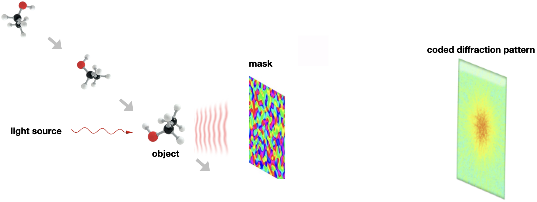
Figure 2. Serial crystallography with a coded aperture

After passing through the object and the mask $\mu$ immediately behind, the exit wave (3)-(4) becomes the masked exit wave $\mu e^{{\rm i}\kappa\psi}$ at the exit plane $z=0$ and then undergoes the free space propagation (with $n=1,f=0$) for $z>0$ described by

$${\rm i}{\partial\over\partial z}v+{1\over 2\kappa}\Delta_{\perp}v=0,\quad v(x,y,0)=\mu e^{{\rm i}\kappa\psi}.$$

The solution is given by convolution with the Fresnel kernel as

$$v(x,y,z) = {1\over{\rm i}\lambda z}\int_{\mathbb{R}^{2}}e^{{{\rm i}\kappa\over 2z}(|x-x^{\prime}|^{2}+|y-y^{\prime}|^{2})}\mu(x^{\prime},y^{\prime})e^{{\rm i}\kappa\psi(x^{\prime},y^{\prime},0)}dx^{\prime}dy^{\prime}$$

and hence, after writing out the quadratic phase term,

(7) $$u(x,y,z) = {e^{{\rm i}\kappa z}\over{\rm i}\lambda z}e^{{{\rm i}\kappa\over 2z}(x^{2}+y^{2})}\int_{\mathbb{R}^{2}}e^{-{{\rm i}\kappa\over z}(xx^{\prime}+yy^{\prime})}e^{{{\rm i}\kappa\over 2z}(|x^{\prime}|^{2}+|y^{\prime}|^{2})}\mu(x^{\prime},y^{\prime})e^{{\rm i}\kappa\psi(x^{\prime},y^{\prime},0)}dx^{\prime}dy^{\prime}.$$

Let the detector plane $z=L$ to be sufficiently far away from the exit plane $z=0$ so that the Fresnel number is small:

(8) $$N_{F}={\ell^{2}\over\lambda L}\ll 1.$$

Then the second integrand (the quadratic phase factor) in (7) is approximately 1 because the integration is carried out in the support of $\mu$ which is taken to be a square of size $\ell$ around the origin. On the other hand, the first integrand in (7) (the cross phase factor) has the effect of the Fourier transform ${\mathcal{F}}$ if the coordinates are properly rescaled to reflect the fact that the detector area is usually much larger than $\ell^{2}$.

Since only the intensities of $u$ are measured, the phase factors $e^{{\rm i}\kappa z}e^{{{\rm i}\kappa\over 2z}(x^{2}+y^{2})}$ in (7) drop out and

(9) $$|u(x,y,L)|^{2}=|v(x,y,L)|^{2}\sim|{\mathcal{F}}[\mu e^{{\rm i}\kappa\psi}]|^{2},$$

up to a scale factor $(\lambda L)^{-1}$, which can be neglected in our analysis.

Depending on the context we shall refer to either a diffraction pattern or a projection as a “snapshot”.

1.2. Contributions

This paper presents a discrete framework for analyzing discrete, finite measurement data analogous to (9) and develops a uniqueness theory for 3D phase retrieval and unwrapping.

Our main contribution in this paper is as follows:

• We introduce pairwise measurement schemes with both coded and un-coded apertures and derive precise conditions for unique determination of (i) the phase projection for strong phase objects (Theorem 3.1 & 3.2) and (ii) the projection, up to a phase factor, for weak phase objects (Theorem 3.4 & 3.5).

• We propose a framework for analyzing the phase unwrapping problem when the given data are phase projections and derive generic conditions for unique phase unwrapping (Theorem 4.1). We provide explicit tilt schemes for phase unwrapping, including, but not limited to, random tilt schemes densely sampled from a spherical triangle with vertexes in three orthogonal directions (Section 4.2.1) and other deterministic tilt schemes (Section 4.2.2)

• We show that any generic set of $n$ projections or generic set of $n+1$ coded diffraction patterns uniquely determine the object (Theorem 5.1 & 5.4).

Our numerical simulation shows that randomly initialized alternating projection algorithm with random tilt schemes can robustly reconstruct 3D objects at high noise levels (Section 6).

1.3. Outline

The rest of the paper can be outlined as follows.

In Section 2, we set up a discrete framework for tomography which is needed for the uniqueness question with finite, discrete measurements.

In Section 3, we prove that with pairwise measurement schemes

(10) $$e^{{\rm i}\kappa g_{\mathbf{t}}} = e^{{\rm i}\kappa f_{\mathbf{t}}}\quad\hbox{in the case of strong phase objects}$$

and, for a constant $\theta_{0}\in\mathbb{R}$,

(11) $$g_{\mathbf{t}} = e^{{\rm i}\theta_{0}}f_{\mathbf{t}}\quad\hbox{ in the case of weak phase objects}$$

if $f,g\in O_{n}$ produce the same diffraction patterns for $\mathbf{t}\in{\mathcal{T}}$, thus reducing 3D phase retrieval to the problem of (phase) projection tomography. In Section 3.3, we introduce pairwise measurement schemes for single-particle imaging where each particle is destroyed after one illumination.

In Section 4 we find conditions on ${\mathcal{T}}$ that ensure $g=f$ if (10) holds. This is a uniqueness theory for phase unwrapping and in Section 4.2 we propose various concrete measurement schemes that conveniently realize the uniqueness conditions.

In Section 5, we find conditions on ${\mathcal{T}}$ that ensure $g=e^{{\rm i}\theta_{0}}f$ for some constant $\theta_{0}\in\mathbb{R}$ independent of $\mathbf{t}$ if (11) holds. This is a unique theory for projection tomography.

In Section 6, we show numerically that with the proposed random tilt measurement scheme alternating projection algorithm can robustly reconstruct a 3D weak-phase object from noisy data of a similar count to that required by the uniqueness theorem.

We discuss the design of 3D tomographic phase unwrapping algorithms and applications to single-particle imaging with unknown orientations in Section 7.

2. Discrete set-up

Imagine an object defined on a cube of size $\ell$ in $\mathbb{R}^{3}$. If we want to discretize the object, what would be a proper grid spacing? Obviously, the finer the grid the higher the fidelity of the discretization. The grid system, however, would be unnecessarily large if the grid spacing is much smaller than the resolution length which is the smallest feature size resolvable by the imaging system.

In a diffraction-limited imaging system such as X-ray crystallography the resolution length is roughly $\lambda/2$. In a radiation-dose-limited system such as electron diffraction, the resolution length can be considerably larger than $\lambda/2$.

Now suppose we choose $\lambda/2$ to be the grid spacing (the voxel size). For this grid system to represent accurately the object continuum, it is necessary that the grid spacing is equal to or smaller than the maximal distance $d$ over which the fractional variation of the object is negligible. On the other hand, the underlying assumption for the paraxial wave equation (1) is exactly $\lambda\leq d$ [53]. Hence the fractional variation of the object within a voxel as well as between adjacent grid points is negligible, two desirable properties of a grid system. In other words, the grid system with spacing $\lambda/2$ gives an accurate representation of the object continuum under the assumption of the paraxial wave equation without resulting in unnecessary complexity.

We will, however, let the discrete object to take independent, arbitrary value in each voxel, except for Section 4 where we assume the so called Itoh condition that the difference in the object between two adjacent grid points is less than $\pi/\kappa$ in order to obtain uniqueness for phase unwrapping.

Let $\lambda/2$ be the unit of length and the grids (the voxels) be labelled by integer triplets $(i,j,k)$. In this length unit, the wavenumber $\kappa$ has the value $\pi$ (i.e. $\pi/\kappa=1$). The number $n$ of grid points in each dimension is about $2\ell/\lambda$ which may be large for a strong phase object.

Let $\llbracket k,l\rrbracket$ denote the integers between and including the integers $k$ and $l$. Let $O_{n}$ denote the class of discrete complex-valued objects

(12) $$O_{n}:=\{f:f(i,j,k)\in\mathbb{C},i,j,k\in\mathbb{Z}_{n}\}$$

where

(15) $$\mathbb{Z}_{n} = \left\{\begin{array}[]{lll}\llbracket-n/2,n/2-1\rrbracket&&\mbox{if $n$ is an even integer;}\\ \llbracket-(n-1)/2,(n-1)/2\rrbracket&&\mbox{if $n$ is an odd integer.}\end{array}\right.$$

To fix the idea, we consider the case of odd $n$ in the paper.

Following the framework in [4] we discretize the projection geometry given in Section 1.1.

We define three families of line segments, the $x$-lines, $y$-lines, and $z$-lines. The $x$-lines, denoted by $\ell_{(1,\alpha,\beta)}(c_{1},c_{2})$ with $|\alpha|,|\beta|<1$, are defined by

(16) $$\ell_{(1,\alpha,\beta)}(c_{1},c_{2}):\left[\begin{matrix}y\\ z\end{matrix}\right]=\left[\begin{matrix}\alpha x+c_{1}\\ \beta x+c_{2}\end{matrix}\right] c_{1},c_{2}\in\mathbb{Z}_{2n-1},\quad x\in\mathbb{Z}_{n}$$

To avoid wraparound of $x$-lines with , we can zero-pad $f$ in a larger lattice $\mathbb{Z}^{3}_{p}$ with $p\geq 2n-1.$ This is particularly important when it comes to define the ray transform by a line sum (cf. (21)-(23)) since wrap-around is unphysical.

Similarly, a $y$-line and a $z$-line are defined as

(17) $$\ell_{(\alpha,1,\beta)}(c_{1},c_{2}):\left[\begin{matrix}x\\ z\end{matrix}\right]=\left[\begin{matrix}\alpha y+c_{1}\\ \beta y+c_{2}\end{matrix}\right] c_{1},c_{2}\in\mathbb{Z}_{2n-1},\quad y\in\mathbb{Z}_{n},$$

(18) $$\ell_{(\alpha,\beta,1)}(c_{1},c_{2}):\left[\begin{matrix}x\\ y\end{matrix}\right]=\left[\begin{matrix}\alpha z+c_{1}\\ \beta z+c_{2}\end{matrix}\right] c_{1},c_{2}\in\mathbb{Z}_{2n-1},\quad z\in\mathbb{Z}_{n},$$

with $|\alpha|,|\beta|<1$.

Let $\widetilde{f}$ be the continuous interpolation of $f$ given by

(19) $$\widetilde{f}(x,y,z) = \sum_{i\in\mathbb{Z}_{n}}\sum_{j\in\mathbb{Z}_{n}}\sum_{k\in\mathbb{Z}_{n}}f(i,j,k)D_{p}(x-i)D_{p}(y-j)D_{p}(z-k),\quad x,y,z,\in\mathbb{R},$$

where $D_{p}$ is the $p$-periodic Dirichlet kernel given by

(20) $$D_{p}(t)={1\over p}\sum_{l\in\mathbb{Z}_{p}}e^{{\rm i}2\pi lt/p} = \left\{\begin{matrix}1,&t=mp,\quad m\in\mathbb{Z}\\ {\sin{(\pi t)}\over p\sin{(\pi t/p)}},&\mbox{else}.\end{matrix}\right.$$

In particular, $[D_{p}(i-j)]_{i,j\in\mathbb{Z}_{p}}$ is the $p\times p$ identity matrix. Because $D_{p}$ is a continuous $p$-periodic function, so is $\widetilde{f}$. However, we will only use the restriction of $\widetilde{f}$ to one period cell $[-(p-1)/2,(p-1)/2]^{3}$ to define the discrete projections and avoid the wraparound effect.

We define the discrete projections as the following line sums

(21) $$f_{(1,\alpha,\beta)}(c_{1},c_{2}) = \sum_{i\in\mathbb{Z}_{n}}\widetilde{f}(i,\alpha i+c_{1},\beta i+c_{2}),$$

(22) $$f_{(\alpha,1,\beta)}(c_{1},c_{2}) = \sum_{j\in\mathbb{Z}_{n}}\widetilde{f}(\alpha j+c_{1},j,\beta j+c_{2})$$

(23) $$f_{(\alpha,\beta,1)}(c_{1},c_{2}) = \sum_{k\in\mathbb{Z}_{n}}\widetilde{f}(\alpha k+c_{1},\beta k+c_{2},k)$$

with $c_{1},c_{2}\in\mathbb{Z}_{2n-1}$.

The 3D discrete Fourier transform $\widehat{f}$ of the object $f\in O_{n}$, is given by

(24) $$\widehat{f}(\xi,\eta,\zeta) = \sum_{i,j,k\in\mathbb{Z}_{n}}f(i,j,k)e^{-{\rm i}2\pi(\xi i+\eta j+\zeta k)/p}=\sum_{i,j,k\in\mathbb{Z}_{p}}f(i,j,k)e^{-{\rm i}2\pi(\xi i+\eta j+\zeta k)/p}$$

where the range of the Fourier variables $\xi,\eta,\zeta$ can be extended from the discrete interval $\mathbb{Z}_{p}$ to the continuum $[-(p-1)/2,(p-1)/2]$. Note that by definition, $\widehat{f}$ is a $p$-periodic band-limited function. The associated 1D and 2D (partial) Fourier transforms are similarly defined $p$-periodic band-limited functions.

2.1. Fourier slices and common lines

The Fourier slice theorem concerns the 2D discrete Fourier transform $\widehat{f}_{(1,\alpha,\beta)}$ defined as

(25) $$\widehat{f}_{(1,\alpha,\beta)}(\eta,\zeta) = \sum_{j,k\in\mathbb{Z}_{2n-1}}f_{(1,\alpha,\beta)}(j,k)e^{-{\rm i}2\pi(\eta j+\zeta k)/p},$$

and the 3D discrete Fourier transform given in (24).

It is straightforward, albeit somewhat tedious, to derive the discrete Fourier slice theorem which plays an important role in our analysis.

Proposition 2.1.

[4] (Discrete Fourier slice theorem) For a given family of $x$-lines $\ell_{(1,\alpha,\beta)}$ with fixed slopes $(\alpha,\beta)$ and variable intercepts $(c_{1},c_{2})$. Then the 2D discrete Fourier transform $\widehat{f}_{(1,\alpha,\beta)}$ of the $x$-projection $f_{(1,\alpha,\beta)},$ given in (21), and the 3D discrete Fourier transform $\widehat{f}$ of the object $f$ satisfy the equation

(26) $$\widehat{f}_{(1,\alpha,\beta)}(\eta,\zeta) = \widehat{f}(-\alpha\eta-\beta\zeta,\eta,\zeta),\quad\eta,\zeta\in\mathbb{Z}.$$

Likewise, we have

(27) $$\widehat{f}_{(\alpha,1,\beta)}(\xi,\zeta) = \widehat{f}(\xi,-\alpha\xi-\beta\zeta,\zeta),\quad\xi,\zeta\in\mathbb{Z};$$

(28) $$\widehat{f}_{(\alpha,\beta,1)}(\xi,\eta) = \widehat{f}(\xi,\eta,-\alpha\xi-\beta\eta).,\quad\xi,\eta\in\mathbb{Z}.$$

Remark 2.2.

For the general domain $\mathbb{R}^{2}$, it is not hard to derive the following results

(29) $$\widehat{f}_{(1,\alpha,\beta)}(\eta,\zeta) = \sum_{j,k\in\mathbb{Z}_{p}}\widehat{f}(-\alpha j-\beta k,j,k)D_{p}(\eta-j)D_{p}(\zeta-k),\quad\eta,\zeta\in\mathbb{R};$$

(30) $$\widehat{f}_{(\alpha,1,\beta)}(\xi,\zeta) = \sum_{j,k\in\mathbb{Z}_{p}}\widehat{f}(\xi,-\alpha j-\beta k,\zeta)D_{p}(\xi-j)D_{p}(\zeta-k),\quad\xi,\zeta\in\mathbb{R};$$

(31) $$\widehat{f}_{(\alpha,\beta,1)}(\xi,\eta) = \sum_{j,k\in\mathbb{Z}_{p}}\widehat{f}(j,k,-\alpha j-\beta k)D_{p}(\xi-j)D_{p}(\eta-k),\quad\eta,\xi\in\mathbb{R},$$

in the form of interpolation by the grids in the respective Fourier slices. From (20) it follows that the right hand side of (29)-(31) are Laurent polynomials of 2 trigonometric variables (e.g. $e^{{\rm i}2\pi\eta/p},e^{{\rm i}2\pi\zeta/p}$ for (29)), and that (29)-(31) reduce to (26)-(28) when the trigonometric variables are integer powers of $e^{{\rm i}2\pi/p}$.

Recalling the view of discretization espoused at the beginning of this section and returning to the original scale in the continuous setting, we note that

(32) $$\lim_{p\to\infty}pD_{p}(pt)=\delta(t),\quad t\in\mathbb{R},$$

the Dirac delta function. By (32) and rescaling the standard, continuous version of Fourier slice theorem is recovered from (29)-(31).

For ease of notation, we denote by $\mathbf{t}$ the direction of projection, $(1,\alpha,\beta),(\alpha,1,\beta)$ or $(\alpha,\beta,1)$ in the reference frame attached to the object. Let $P_{\mathbf{t}}$ denote the origin-containing (continuous) plane orthogonal to $\mathbf{t}$ in the Fourier space. The standard common line is defined by $L_{\mathbf{t},\mathbf{t}^{\prime}}:=P_{\mathbf{t}}\cap P_{\mathbf{t}^{\prime}}$ for $\mathbf{t},\mathbf{t}^{\prime}$ not parallel to each other.

By a slight abuse of notation, the common-line property implied by Proposition 2.1 can be succinctly stated as

(33) $$\widehat{f}_{\mathbf{t}}({\mathbf{k}}) = \widehat{f}_{\mathbf{t}^{\prime}}({\mathbf{k}}^{\prime}),\quad{\mathbf{k}}\in P_{\mathbf{t}}\cap\mathbb{Z}^{2},\quad{\mathbf{k}}^{\prime}\in P_{\mathbf{t}^{\prime}}\cap\mathbb{Z}^{2},$$

where ${\mathbf{k}},{\mathbf{k}}^{\prime}$ are the corresponding coordinates and may differ from each other depending on the parametrization of $P_{\mathbf{t}}$ and $P_{\mathbf{t}^{\prime}}$.

For example, let $\mathbf{t}\sim(\alpha,\beta,1)$ and $\mathbf{t}^{\prime}\sim(\alpha^{\prime},\beta^{\prime},1)$. The Fourier slices are given by

(34) $$\alpha\xi+\beta\eta+\zeta=0,\quad\alpha^{\prime}\xi+\beta^{\prime}\eta+\zeta=0,$$

with the correspondence ${\mathbf{k}}={\mathbf{k}}^{\prime}=(\xi,\eta)\in\mathbb{Z}^{2}$.

For a different configuration, let $\mathbf{t}\sim(\alpha,\beta,1)$ and $\mathbf{t}^{\prime}\sim(1,\beta^{\prime},\gamma^{\prime})$. The Fourier planes are given by

(35) $$\alpha\xi+\beta\eta+\zeta=0,\quad\xi+\beta^{\prime}\eta+\gamma^{\prime}\zeta=0,$$

with the correspondence ${\mathbf{k}}=(\xi,\eta)\in\mathbb{Z}^{2}$ and ${\mathbf{k}}^{\prime}=(\eta,\zeta)\in\mathbb{Z}^{2}$.

For non-integral points, however, the common lines are perturbed by interpolation (29)-(31). For (34) and (35), the “common lines” can be generalized respectively as the traces of the two-dimensional surfaces defined by

(36) $$L_{\mathbf{t},\mathbf{t}^{\prime}}(f) := \Big{\{}\widehat{f}_{(\alpha,\beta,1)}(\xi,\eta)=\widehat{f}_{(\alpha^{\prime},\beta^{\prime},1)}(\xi^{\prime},\eta^{\prime})\Big{\}}\subseteq\mathbb{R}^{2}\times\mathbb{R}^{2}$$

(37) $$L_{\mathbf{t},\mathbf{t}^{\prime}}(f) := \Big{\{}\widehat{f}_{(\alpha,\beta,1)}(\xi,\eta)=\widehat{f}_{(1,\beta^{\prime},\gamma^{\prime})}(\eta^{\prime},\zeta^{\prime})\Big{\}}\subseteq\mathbb{R}^{2}\times\mathbb{R}^{2}.$$

By the common line property (33), $L_{\mathbf{t},\mathbf{t}^{\prime}}$ in (36) contains the set defined by $(\xi^{\prime},\eta^{\prime})=(\xi,\eta)\in\mathbb{Z}^{2}$ while $L_{\mathbf{t},\mathbf{t}^{\prime}}$ in (37) contains the set defined by

(38) $$\eta^{\prime}=\eta,\quad\zeta^{\prime}=-\alpha\xi-\beta\eta\in\mathbb{Z},\quad(1-\alpha\gamma^{\prime})\xi=(\beta\gamma^{\prime}-\beta^{\prime})\eta,\quad(\xi,\eta)\in\mathbb{Z}^{2}.$$

By (33), $0\in L_{\mathbf{t},\mathbf{t}^{\prime}}(f)$ for any $\mathbf{t},\mathbf{t}^{\prime}$. In view of (32), the trace of $L_{\mathbf{t},\mathbf{t}^{\prime}}$ on either Fourier slice is near $P_{\mathbf{t}}\cap P_{\mathbf{t}^{\prime}}$ for sufficiently large $n$.

We shall refer to $L_{\mathbf{t},\mathbf{t}^{\prime}}(f)$ as the common set for the Fourier slices of $f$ orthogonal to $\mathbf{t},\mathbf{t}^{\prime}$. The notion of common sets will be used to formulate a technical condition for Theorem 3.2.

2.2. Diffraction pattern

Let ${\mathcal{T}}$ denote the set of directions $\mathbf{t}$ employed in the 3D diffraction measurement, which can be coded (as in Figure 2) or uncoded (as in Figure 1). To fix the idea, let $p=2n-1$ in (20).

Let the Fourier transform ${\mathcal{F}}$ of the projection $e^{{\rm i}\kappa f_{\mathbf{t}}({\mathbf{n}})}$ be written as

(39) $$F_{\mathbf{t}}(e^{-{\rm i}2\pi\mathbf{w}})=\sum_{{\mathbf{n}}\in\mathbb{Z}_{p}^{2}}e^{-{\rm i}2\pi{\mathbf{n}}\cdot\mathbf{w}}e^{{\rm i}\kappa f_{\mathbf{t}}({\mathbf{n}})},\quad\mathbf{w}\in\Big{[}-{1\over 2},{1\over 2}\Big{]}^{2}.$$

In the absence of a random mask ($\mu\equiv 1$), the intensities of the Fourier transform can be written as

(40) $$|F_{\mathbf{t}}(e^{-{\rm i}2\pi\mathbf{w}})|^{2}=\sum_{{\mathbf{n}}\in\mathbb{Z}_{2p-1}^{2}}\left\{\sum_{{\mathbf{n}}^{\prime}\in\mathbb{Z}_{p}^{2}}e^{{\rm i}\kappa f_{\mathbf{t}}({\mathbf{n}}^{\prime}+{\mathbf{n}})}e^{-{\rm i}\kappa\overline{f_{\mathbf{t}}({\mathbf{n}}^{\prime})}}\right\}e^{-{\rm i}2\pi{\mathbf{n}}\cdot\mathbf{w}},\quad\mathbf{w}\in\Big{[}-{1\over 2},{1\over 2}\Big{]}^{2},$$

which is called the uncoded diffraction pattern in the direction $\mathbf{t}$. Here and below the over-line notation means complex conjugacy. The expression in the brackets in (40) is the autocorrelation function of $e^{{\rm i}\kappa f_{\mathbf{t}}}$.

The diffraction patterns are then uniquely determined by sampling on the grid

(41) $$\mathbf{w}\in{1\over 2p-1}\mathbb{Z}_{2p-1}^{2}$$

or by Kadec’s $1/4$-theorem on any following irregular grid [97]

(42) $$\{\mathbf{w}_{jk},\,\,j,k\in\mathbb{Z}_{2p-1}:|(2p-1)\mathbf{w}_{jk}-(j,k)|<1/4\}.$$

With the regular (41) or irregular (42) sampling, the diffraction pattern contains the same information as does the autocorrelation function of $f_{\mathbf{t}}$.

3. Pairwise reduction to (phase) projection

We assume the following on the coded aperture

Mask Assumption: The mask function is given by $\mu({\mathbf{n}})=\exp[{\rm i}\phi({\mathbf{n}})]$ with independent, continuous random variables $\phi({\mathbf{n}})\in\mathbb{R}$.

Let $f^{*}_{\mathbf{t}}$ denote the projection $f_{\mathbf{t}}$ translated by some ${\mathbf{l}}_{\mathbf{t}}\in\mathbb{Z}^{2}$, i.e.

(43) $$f^{*}_{\mathbf{t}}({\mathbf{n}}):=f_{\mathbf{t}}({\mathbf{n}}+{\mathbf{l}}_{\mathbf{t}}),\quad\quad\hbox{subject to}\,\,{\hbox{\rm supp}}(f^{*}_{\mathbf{t}})\subseteq\mathbb{Z}_{n}^{2}.$$

We assume that each snapshot is taken for $f^{*}_{\mathbf{t}}$ (not $f_{\mathbf{t}}$) with a shift ${\mathbf{l}}_{\mathbf{t}}$ due to variability in sample delivery.

In Section 3.1 and 3.2, we show for two different imaging geometries how a pair of diffraction patterns can uniquely determine the respective (phase) projections.

3.1. Strong phase objects

The following theorem says that the two diffraction patterns, one coded and one uncoded, uniquely determine the underlying phase projection.

Theorem 3.1.

Let $f,g\in O_{n}$ and assume the Mask Assumption. Suppose that for any $\mathbf{t}$

(44) $$|{\mathcal{F}}(e^{{\rm i}\kappa g^{*}_{\mathbf{t}}})|^{2} = |{\mathcal{F}}(e^{{\rm i}\kappa f^{*}_{\mathbf{t}}})|^{2}$$

(45) $$|{\mathcal{F}}(\mu\odot e^{{\rm i}\kappa g^{*}_{\mathbf{t}}})|^{2} = |{\mathcal{F}}(\mu\odot e^{{\rm i}\kappa f^{*}_{\mathbf{t}}})|^{2}$$

Then $e^{{\rm i}\kappa g_{\mathbf{t}}}=e^{{\rm i}\kappa f_{\mathbf{t}}}$ almost surely.

The proof of Theorem 3.1 is given in Appendix A.

The next theorem says that the two coded diffraction patterns in two different directions uniquely determine the two corresponding phase projections.

Theorem 3.2.

Let $f,g\in O_{n}$ such that for $\mathbf{t},\mathbf{t}^{\prime}$ not parallel to each other, the intersection $C_{\mathbf{t},\mathbf{t}^{\prime}}:=L_{\mathbf{t},\mathbf{t}^{\prime}}(f)\cap L_{\mathbf{t},\mathbf{t}^{\prime}}(g)$ contains some $({\mathbf{k}},{\mathbf{k}}^{\prime})\neq 0$ such that the slope of either ${\mathbf{k}}$ or ${\mathbf{k}}^{\prime}$ is not a fraction over $\mathbb{Z}_{p}$. Let the Mask Assumption hold true. Suppose that

(46) $$|{\mathcal{F}}(\mu\odot e^{{\rm i}\kappa g^{*}_{\mathbf{t}^{\prime}}})|^{2} = |{\mathcal{F}}(\mu\odot e^{{\rm i}\kappa f^{*}_{\mathbf{t}^{\prime}}})|^{2}$$

(47) $$|{\mathcal{F}}(\mu\odot e^{{\rm i}\kappa g^{*}_{\mathbf{t}}})|^{2} = |{\mathcal{F}}(\mu\odot e^{{\rm i}\kappa f^{*}_{\mathbf{t}}})|^{2}.$$

Then $e^{{\rm i}\kappa g_{\mathbf{t}}}=e^{{\rm i}\kappa f_{\mathbf{t}}}$ and $e^{{\rm i}\kappa g_{\mathbf{t}^{\prime}}}=e^{{\rm i}\kappa f_{\mathbf{t}^{\prime}}}$ almost surely.

The proof of Theorem 3.2 is given in Appendix B.

Corollary 3.3.

If for each $\mathbf{t}\in{\mathcal{T}}$ there is a $\mathbf{t}^{\prime}\in{\mathcal{T}}$ to satisfy Theorem 3.2, then $e^{{\rm i}\kappa g_{\mathbf{t}}}=e^{{\rm i}\kappa f_{\mathbf{t}}}$ for all $\mathbf{t}\in{\mathcal{T}}$.

Note that Theorem 3.1, 3.2 and Corollary 3.3 do not hold for a uniform mask ($\mu=$ cost.) because the chiral ambiguity and the shift ambiguity are present, i.e. both $g(\cdot)=f(-\cdot)$ and $g(\cdot)=f(\cdot+{\mathbf{l}}),{\mathbf{l}}\in\mathbb{R}^{3},$ satisfy all the assumptions therein but $e^{{\rm i}\kappa g_{\mathbf{t}}}\not\equiv e^{{\rm i}\kappa f_{\mathbf{t}}}$ in general.

Analogous results can be formulated for the hybrid approximation (6) but we will omit the details here. Instead, we will present the dark-field imaging under the weak-phase-object approximation next.

3.2. Weak phase objects

Under the weak-phase-object assumption (5) the exit wave is given by

(48) $$v_{B}(x,y)=1-{{\rm i}\over 2\kappa}\int dz^{\prime}{f(x,y,z^{\prime})}.$$

The coded diffraction pattern of the exit wave is given by

(49) $$|{\mathcal{F}}(\mu\odot v_{B})|^{2} = |{\mathcal{F}}\mu|^{2}+{1\over\kappa}\Im\{{\overline{{\mathcal{F}}\mu}\cdot{\mathcal{F}}(\mu\int fdz^{\prime})}\}+{1\over 4\kappa^{2}}|{\mathcal{F}}(\mu\int fdz^{\prime})|^{2}$$

where $\Im$ denotes the imaginary part.

As (49) represents the interference pattern between the reference wave ${\mathcal{F}}(\mu)$ and the masked object wave $-{\rm i}{\mathcal{F}}(\mu\int fdz^{\prime})/(2\kappa)$, reconstruction based on the second term on the right hand side of (49) can be performed by conventional holographic techniques [63, 94, 95].

We take the diffraction patterns of the scattered waves

(50) $$|{\mathcal{F}}(\mu\odot f_{\mathbf{t}})|^{2},$$

as measurement data, which is reminiscent of dark-field imaging in light and electron microscopies where the unscattered wave (i.e. ${\mathcal{F}}\mu$) is removed from view [34, 2]. Dark-field imaging mode arises naturally in X-ray coherent diffractive imaging due to the use of a beam stop for blocking the direct beam in order to protect the detector and enhance the measurement of weakly scattered intensities.

The next two theorems are analogous to Theorem 3.1 and 3.2. A notable effect of the dark-field imaging is the appearance of an undetermined phase factor absent in Theorem 3.1 and 3.2.

Theorem 3.4.

Let $f,g\in O_{n}$ and assume the Mask Assumption. Suppose that ${\hbox{\rm supp}}(f_{\mathbf{t}})$ is not a subset of a line and that

(51) $$|{\mathcal{F}}(g^{*}_{\mathbf{t}})|^{2} = |{\mathcal{F}}(f^{*}_{\mathbf{t}})|^{2}$$

(52) $$|{\mathcal{F}}(\mu\odot g^{*}_{\mathbf{t}})|^{2} = |{\mathcal{F}}(\mu\odot f^{*}_{\mathbf{t}})|^{2}$$

Then almost surely ${g_{\mathbf{t}}}=e^{{\rm i}\theta_{\mathbf{t}}}f_{\mathbf{t}}$ for some constant $\theta_{\mathbf{t}}\in\mathbb{R}$.

The proof of Theorem 3.4 is given in Appendix C.

Theorem 3.5.

Let $f,g\in O_{n}$ and suppose that $\widehat{f}(0)\neq 0$. Let the Mask Assumption hold true. Suppose that neither ${\hbox{\rm supp}}(f_{\mathbf{t}})$ nor ${\hbox{\rm supp}}(f_{\mathbf{t}^{\prime}})$ is a subset of a line and that

(53) $$|{\mathcal{F}}(\mu\odot g^{*}_{\mathbf{t}^{\prime}})|^{2} = |{\mathcal{F}}(\mu\odot f^{*}_{\mathbf{t}^{\prime}})|^{2}$$

(54) $$|{\mathcal{F}}(\mu\odot g^{*}_{\mathbf{t}})|^{2} = |{\mathcal{F}}(\mu\odot f^{*}_{\mathbf{t}})|^{2}$$

where $\mathbf{t}$ and $\mathbf{t}^{\prime}$ are not parallel to each other. Then almost surely

(55) $$\hbox{either}\quad\left({g_{\mathbf{t}}}=e^{{\rm i}\theta_{0}}f_{\mathbf{t}}\quad\&\quad g_{\mathbf{t}^{\prime}}=e^{{\rm i}\theta_{0}}f_{\mathbf{t}^{\prime}}\right)\quad\hbox{or}\quad f^{*}_{\mathbf{t}}=f^{*}_{\mathbf{t}^{\prime}},$$

for some constant $\theta_{0}\in\mathbb{R}$ (the two in (55) may both be true).

Corollary 3.6.

Let the assumptions of Theorem 3.5 hold for any two non-parallel $\mathbf{t},\mathbf{t}^{\prime}\in{\mathcal{T}}$. Then

(56) $$\hbox{either}\quad\left({g_{\mathbf{t}}}=e^{{\rm i}\theta_{0}}f_{\mathbf{t}},\quad\forall\mathbf{t}\in{\mathcal{T}}\right)\quad\hbox{or}\quad(f^{*}_{\mathbf{t}}=f^{*}_{\mathbf{t}^{\prime}},\quad\forall\mathbf{t},\mathbf{t}^{\prime}\in{\mathcal{T}})$$

where $\theta_{0}$ is independent of $\mathbf{t}\in{\mathcal{T}}$.

Proof.

First, let us make the following observation. Suppose ${g_{\mathbf{t}}}=e^{{\rm i}\theta_{\mathbf{t}}}f_{\mathbf{t}}$ and ${g_{\mathbf{t}^{\prime}}}=e^{{\rm i}\theta_{\mathbf{t}^{\prime}}}f_{\mathbf{t}^{\prime}}$ for $\mathbf{t}\neq\mathbf{t}^{\prime}$. By Proposition 2.1 $\widehat{f}_{\mathbf{t}}(0)=\widehat{f}_{\mathbf{t}^{\prime}}(0)=\widehat{f}(0)\neq 0,$ it follows from $\widehat{g}_{\mathbf{t}}(0)=\widehat{g}_{\mathbf{t}^{\prime}}(0)$ that $\theta_{\mathbf{t}}=\theta_{\mathbf{t}^{\prime}}$.

Consequently, let ${\mathcal{T}}_{1}\subseteq{\mathcal{T}}$ be the maximum set of all $\mathbf{t}\in{\mathcal{T}}$ for which ${g_{\mathbf{t}}}=e^{{\rm i}\theta_{0}}f_{\mathbf{t}}$ for $\theta_{0}\in\mathbb{R}$ independent of $\mathbf{t}\in{\mathcal{T}}$. Note that the value of $\theta_{0}$ is arbitrary. Since ${\mathcal{T}}_{1}$ is maximal, it follows that $g_{\mathbf{t}^{\prime}}\neq e^{{\rm i}\theta_{0}}f_{\mathbf{t}^{\prime}}$ for any $\mathbf{t}^{\prime}\not\in{\mathcal{T}}_{1}$.

Suppose the first alternative in (56) is not true, i.e. ${\mathcal{T}}_{1}\neq{\mathcal{T}}$. Consider any $\mathbf{t}^{\prime}\not\in{\mathcal{T}}_{1}$ and $\mathbf{t}\in{\mathcal{T}}_{1}$. By Theorem 3.5, $f^{*}_{\mathbf{t}}=f^{*}_{\mathbf{t}^{\prime}},$ implying the second alternative in (56).

∎

3.3. Pairwise measurement for single-particle imaging

(a) Beam splitter with coded and uncoded apertures

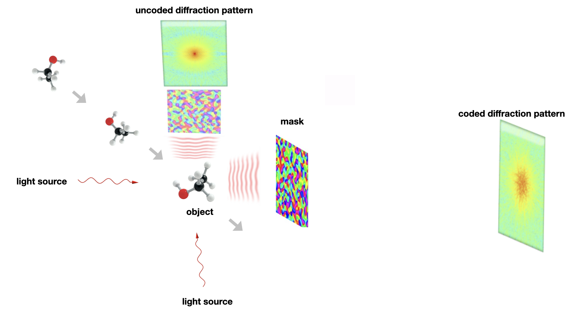
(b) Two coded apertures in a known relative orientation

Figure 3. (a) Simultaneous measurement of one coded and one uncoded diffraction patterns with a beam splitter; (b) Simultaneous illumination of the object with two coded apertures in a known relative orientation.

In this section, we introduce pairwise measurement schemes for single-particle imaging where each particle is destroyed after one illumination [10, 12, 56]. How can two diffraction patterns be measured, as assumed by Theorem 3.1, 3.2, 3.4 and 3.5, if the particle is illuminated only once?

3.3.1. Beam splitter

For Theorem 3.1 & 3.4 with a unknown $\mathbf{t}$, how can we be sure that the coded and uncoded diffraction patterns are measured in the same direction?

Consider the measurement scheme stylized in Figure 3(a) where a beam splitter is inserted behind the object and the mask placed in only one of two light paths behind the splitter. Ideally, the beam splitter produces two identical beams to facilitate two snapshots of the same exit wave. The reader is referred to [74, 59, 61, 79] for recent advances in X-ray splitters.

3.3.2. Dual illuminations

For Theorem 3.2 & 3.5 we need a physical set-up that can render a pair of diffraction patterns in two different directions. This can be achieved by simultaneous illuminations by two beams with both exit waves masked by the coded aperture as depicted in Figure 3(b). Note that the two beams need not be coherent with each other since no interference between the two is called for.

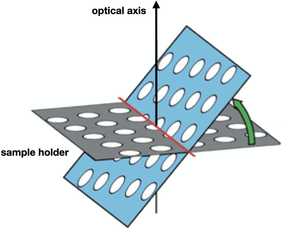
(a) Tilt geometry for sequential illuminations

Figure 4. Serial data collection implemented by the random conical tilt and orthogonal tilt in cryo-EM both of which collect pairs of measurement data in a fixed relative orientation corresponding to the angle about $50\deg$ and $90\deg$, respectively, between the two beams[34, 60].

If the particles can endure more than one dose of radiation then a fixed-target sample delivery can be implemented by the cryo-EM scheme random conical tilt (RCT) or orthogonal tilt (OT) [34, 60]. As shown in Figure 4, many identical particles are randomly located and oriented on a grid which can be precisely tilted about a tilt axis by a goniometer. With dose-fractionated beams, the diffraction patterns of the identical particles in the two orientations are measured with the coded aperture in correspondence with Figure 3(b).

Because only one exit wave is aimed at in Figure 3(a) instead of two in Figure 3(b), the exit wave reconstruction as guaranteed by Theorem 3.1 and 3.4 would be much more effective and robust than that guaranteed by Theorem 3.2 and 3.5. Indeed, the exit wave reconstruction from the two diffraction patterns collected in Figure 3(a) is equivalent to the phase retrieval problem well studied previously [28, 15, 31].

3.4. Sector constraint

The X-ray spectrum generally lies to the high-frequency side of various resonances associated with the binding of electrons so the complex refractive index can be written as

(57) $$n=1-\delta+{\rm i}\beta,\quad 0<\delta,\beta\ll 1,$$

where $\delta$ and $\beta$, respectively, describe the dispersive and absorptive aspects of the wave-matter interaction. The component $\beta$ is usually much smaller than $\delta$ which is often of the order of $10^{-5}$ for X-rays [55, 76].

By (4) and (57),

(58) $$f={1\over 2}(n^{2}-1)\approx-\delta+{\rm i}\beta$$

and hence $f$ satisfies the so called sector condition introduced in [25], i.e. the phase angle $\angle f({\mathbf{n}})$ of $f_{\mathbf{t}}({\mathbf{n}})$ for each ${\mathbf{n}}$ satisfies

(59) $$\angle f({\mathbf{n}})\in[a,b],\quad|a-b|<2\pi,$$

where $a$ and $b$ are two constants independent of ${\mathbf{n}}$. For example, for $\beta\geq 0$, $a=0$ and $b=\pi$. In particular, if $\beta\ll\delta>0$, then $a\approx\pi$ and $b=\pi$. The sector condition is a generalization of the constraint of positivity (of electron density) which is the cornerstone of the “direct methods” in X-ray crystallography [44].

In view of (32), the continuous interpolation $\widetilde{f}$ in (19) satisfies the sector condition

(60) $$\angle\widetilde{f}({\mathbf{n}})\in[\tilde{a},\tilde{b}]\quad(\tilde{a}\approx a,\,\,\tilde{b}\approx b,\,\,p\gg 1).$$

If $|\tilde{b}-\tilde{a}|\leq\pi,$ the sector (60) is a convex set and hence the discrete projections (21)-(23) also satisfy the section condition (60). However, we can not expect the phase projection $e^{{\rm i}\kappa f_{\mathbf{t}}}$ to satisfy the sector condition regardless of $|\tilde{b}-\tilde{a}|$.

The sector condition (59) enables reduction from a single coded diffraction pattern for a weak-phase object as stated below.

Theorem 3.7.

[25] Let $f\in O_{n}$ with the singleton ${\mathcal{T}}=\{\mathbf{t}\}$ for any $\mathbf{t}$ such that the sector condition (60) is convex (i.e. $|\tilde{b}-\tilde{a}|\leq\pi$). Assume the mask function $\mu({\mathbf{n}})=\exp[{\rm i}\phi({\mathbf{n}})]$ to be uniformly distributed over the unit circle. Suppose that ${\hbox{\rm supp}}(f_{\mathbf{t}})$ is not a subset of a line and that for $g\in O_{n}$, $g^{*}_{\mathbf{t}}$ produces the same coded diffraction pattern as $f^{*}_{\mathbf{t}}$. Then with probability at least

(61) $$1-n^{2}\left|{\tilde{b}-\tilde{a}\over 2\pi}\right|^{\lfloor S_{\mathbf{t}}/2\rfloor}\geq 1-n^{2}2^{-\lfloor S_{\mathbf{t}}/2\rfloor},$$

where $S_{\mathbf{t}}$ is the number of nonzero pixels of $f_{\mathbf{t}}$, we have ${g_{\mathbf{t}}}=e^{{\rm i}\theta_{\mathbf{t}}}f_{\mathbf{t}}$ for some constant $\theta_{\mathbf{t}}\in\mathbb{R}.$

If $|{\mathcal{T}}|>1$ and if the mask functions for different $\mathbf{t}\in{\mathcal{T}}$ are independently distributed, then the probability for Theorem 3.7 to hold for all $\mathbf{t}\in{\mathcal{T}}$ is at least

$$\prod_{\mathbf{t}\in{\mathcal{T}}}\left(1-n^{2}\left|{\tilde{b}-\tilde{a}\over 2\pi}\right|^{\lfloor S_{\mathbf{t}}/2\rfloor}\right).$$

For the sake of simplicity in measurement, however, let $\mu$ be the same mask for all $\mathbf{t}\in{\mathcal{T}}$. The probability for Theorem 3.7 to hold for all $\mathbf{t}\in{\mathcal{T}}$ can be roughly estimated as follows.

First note that for any two events $A$ and $B$,

(62) $$P(A\cap B)=P(A)+P(B)-P(A\cap B)\geq P(A)+P(B)-1,$$

where $P(\cdot)$ is the probability of the respective event. Let ${\mathcal{T}}=\{\mathbf{t}_{j}:j=1,...,m\}$, $E_{j}$ be the event that Theorem 3.7 to hold for $\mathbf{t}_{j}$ and $p_{j}=P(E_{j})$. By Theorem 3.7, $p_{j}\geq 1-c_{j}$ where

$$c_{j}=n^{2}\left|{\tilde{b}-\tilde{a}\over 2\pi}\right|^{\lfloor S_{\mathbf{t}_{j}}/2\rfloor},$$

and, hence by (62),

(63) $$P(E_{1}\cap E_{2})\geq p_{1}+p_{2}-1\geq 1-2c,\quad c=\max_{j}c_{j}.$$

Iterating the bound (62) inductively with $E_{j},j=1,...,m$, we obtain

$$P(\cap_{i=1}^{m}E_{i})=P(\cap_{i=1}^{m-1}E_{i}\cap E_{m})\geq 1-(m-1)c-c=1-mc.$$

Corollary 3.8.

Suppose $\widehat{f}(0)\neq 0$. Theorem 3.7 holds true for $\mathbf{t}$ with the same constant $\theta_{\mathbf{t}}=\theta_{0}\in\mathbb{R}$ independent of $\mathbf{t}$ in any ${\mathcal{T}}$ with probability at least

(64) $$1-|{\mathcal{T}}|n^{2}\left|{\tilde{b}-\tilde{a}\over 2\pi}\right|^{s/2},\quad s:=\min_{j}S_{\mathbf{t}_{j}},$$

where $s$ is the minimum sparsity (the least number of nonzero pixels) in all directions in ${\mathcal{T}}$.

Proof.

By Proposition 2.1 $\widehat{f}_{\mathbf{t}}(0)=\widehat{f}_{\mathbf{t}^{\prime}}(0)=\widehat{f}(0)\neq 0,$ it follows from $\widehat{g}_{\mathbf{t}}(0)=\widehat{g}_{\mathbf{t}^{\prime}}(0)$ that $\theta_{\mathbf{t}}=\theta_{\mathbf{t}^{\prime}}$. Namely, $g_{\mathbf{t}}=e^{{\rm i}\theta_{0}}f_{\mathbf{t}}$ for some constant $\theta_{0}$ independent of $\mathbf{t}\in{\mathcal{T}}$.

The proof is complete. ∎

The bound (64) is meaningful only if

(65) $$|{\mathcal{T}}|<n^{-2}\left|{\tilde{b}-\tilde{a}\over 2\pi}\right|^{-s/2}.$$

Usually $s$ is at least a multiple of $n$ (often ${\mathcal{O}}(n^{2})$), (65) allows nearly exponentially large number of projections. As we will see in Corollary 5.3 (ii), a far smaller number $m=n$ of projections suffices for unique determination of a weak phase object.

Note that Theorem 3.4, 3.5, 3.7, Corollary 3.3 and 3.8 do not hold for a uniform mask ($\mu=$ cost.) because the chiral ambiguity and the shift ambiguity are present, i.e. both $g(\cdot)=f(-\cdot)$ and $g(\cdot)=f(\cdot+{\mathbf{l}}),{\mathbf{l}}\in\mathbb{Z}^{3},$ satisfy all the assumptions therein but $g_{\mathbf{t}}\not\equiv e^{{\rm i}\theta_{\mathbf{t}}}f_{\mathbf{t}}$ in general.

4. Phase unwrapping

For a strong phase object, (10) naturally leads to the problem of phase unwrapping:

(66) $$g_{\mathbf{t}}({\mathbf{n}})=f_{\mathbf{t}}({\mathbf{n}})\quad\mod 2\pi/\kappa,\quad{\mathbf{n}}\in\mathbb{Z}_{p}^{2},$$

which may have infinitely many solutions. We seek conditions on ${\mathcal{T}}$ that can uniquely determine the 3D object in the sense that $g\equiv f.$

A basic approach appeals to the continuity of the projection’s dependence on the direction $\mathbf{t}$, which, in turn, is the consequence of continuous interpolation (19).

Let ${\mathcal{T}}_{\epsilon}$ denote the graph with the nodes given by $\mathbf{t}\in{\mathcal{T}}$ and the edges defined between any two nodes $\mathbf{t}_{1},\mathbf{t}_{2}\in{\mathcal{T}}$ with $|\angle\mathbf{t}_{1}\mathbf{t}_{2}|\leq\epsilon$ (such edges are called $\epsilon$-edges) where $\angle\mathbf{t}_{1}\mathbf{t}_{2}$ is the angle between $\mathbf{t}_{1}$ and $\mathbf{t}_{2}$. We call ${\mathcal{T}}$ is $\epsilon$-connected if ${\mathcal{T}}_{\epsilon}$ is a connected graph. We say that two nodes $\mathbf{t}_{1},\mathbf{t}_{2}$ are $\epsilon$-connected if there is an $\epsilon$-edge between them.

Suppose that ${\mathcal{T}}$ is $\epsilon$-connected for certain $\epsilon$ (to be determined later). The continuous dependence of $g_{\mathbf{t}},f_{\mathbf{t}}$ on $\mathbf{t}$ implies that $|g_{\mathbf{t}_{1}}-g_{\mathbf{t}_{2}}|$ and $|f_{\mathbf{t}_{1}}-f_{\mathbf{t}_{2}}|$ are arbitrarily small if $\angle\mathbf{t}_{1}\mathbf{t}_{2}$ is sufficiently small. On the other hand, $h_{\mathbf{t}_{1}}-h_{\mathbf{t}_{2}}$ is an integer multiple of $2\pi/\kappa$ where $h_{\mathbf{t}}:=g_{\mathbf{t}}-f_{\mathbf{t}}$. Then for sufficiently small $\epsilon$, $h_{\mathbf{t}}({\mathbf{n}})$ is a constant for each ${\mathbf{n}}$ and hence $g_{\mathbf{t}}-f_{\mathbf{t}}$ is independent of $\mathbf{t}$.

We can give a rough estimate for the required closeness $\epsilon$ of two adjacent projections as follows. In general, the gradient of the continuous extension $\widetilde{f}$ is ${\mathcal{O}}(1)$ and hence the gradient of $f_{\mathbf{t}}$ (being a sum of $n$ values of $f$) with respect to $\mathbf{t}$ is ${\mathcal{O}}(n)$. Consequently, $|f_{\mathbf{t}_{1}}-f_{\mathbf{t}_{2}}|$ can be made sufficiently small with $\epsilon={\mathcal{O}}(1/n)$ (with a sufficiently small constant).

As pointed out at the beginning of Section 2, if we make use of the property that the fractional variation of $f$ between adjacent grids is negligible, then the gradient of the continuous extension $\widetilde{f}$ is $o(1)$ and $|f_{\mathbf{t}_{1}}-f_{\mathbf{t}_{2}}|$ can be made sufficiently small with $\epsilon$ that may be much larger than $1/n.$

The main result of this section will need the diversity condition:

(67) $$\#\{\alpha_{l}\xi+\beta_{l}\eta:|\alpha_{l}|,|\beta_{l}|<1,\,\,l=1,\dots,n\}=n\hbox{ for each $\xi,\eta\in\mathbb{Z}_{p},$ $(\xi,\eta)\neq 0$}.$$

In other words, the difference $(\alpha_{l}-\alpha_{k},\beta_{l}-\beta_{k}),l\neq k,$ is not expressible as $Z_{p}$-fractions.

Theorem 4.1.

Let ${\mathcal{T}}$ be an $\epsilon$-connected set of directions containing any of the following three sets:

(68) $$\{(1,\alpha_{l},\beta_{l}):l=1,\dots,n\}\cup\{(0,\alpha_{0},\beta_{0}),(0,0,1)\}$$

(69) $$\{(\beta_{l},1,\alpha_{l}):l=1,\dots,n\}\cup\{(\beta_{0},0,\alpha_{0}),(1,0,0)\}$$

(70) $$\{(\alpha_{l},\beta_{l},1):l=1,\dots,n\}\cup\{(\alpha_{0},\beta_{0},0),(0,1,0)\}$$

under the assumption (67) and that $\alpha_{0}\neq 0,|\beta_{0}|<1$.

Suppose that the maximum variation of the object $f$ between two adjacent grid points is less than $\pi/\kappa$ (The 3D Itoh condition) and (10) holds for a sufficiently small $\epsilon={\mathcal{O}}(1/n)$. Then $g=f$.

Remark 4.2.

As per the discussion in Section 2, with $\lambda/2$ as the unit of length, $\pi/\kappa=1$.

The projection $f_{\mathbf{t}}$ in a direction $\mathbf{t}$, however, usually violates the 2D Itoh condition. Hence 2D phase unwrapping for $f_{\mathbf{t}}$ may not have a unique solution [54, 39].

Remark 4.3.

As shown in the following proof, the $x,y$ and $z$ axes in (68), (69) and (70), respectively, show up in the analysis because they are “privileged” w.r.t. $\mathbb{Z}_{n}^{3}$ which is not isotropic. On the other hand, due to arbitrariness in choosing the orientation of the object frame, we can always designate one of the projection directions in ${\mathcal{T}}$ as exactly one of the coordinate axes, say, (0,0,1), and discretize the object domain into $\mathbb{Z}_{n}^{3}$ accordingly.

Proof.

It suffices to consider the case that ${\mathcal{T}}$ contains the set (68).

Let (66) hold true. Then the $\epsilon$-connected schemes with sufficiently small $\epsilon$ ensure

$$h_{\mathbf{t}}({\mathbf{n}}):=g_{\mathbf{t}}({\mathbf{n}})-f_{\mathbf{t}}({\mathbf{n}})\quad\hbox{is independent of $\mathbf{t}\in{\mathcal{T}}$}.$$

Intuitively, with sufficiently diverse views in ${\mathcal{T}}$, $h:=g-f$ must be a multiple of Kronecker’s delta function as shown in the following analysis.

Let $c(\cdot,\cdot)$ be independent of $\alpha_{l},\beta_{l},$ such that

(71) $$\widehat{h}_{(1,\alpha_{l},\beta_{l})}(\eta,\zeta) = c(\eta,\zeta)$$

and hence by Fourier Slice Theorem

(72) $$\widehat{h}(-\eta,\zeta\in\mathbb{Z}\alpha_{l}\eta-\beta_{l}\zeta,\eta,\zeta) = c(\eta,\zeta),\quad\eta,\zeta\in\mathbb{Z}_{p}.$$

We want to show $c\equiv 0$.

Define the notation:

(73) $$\widehat{h}_{\eta}(m,l) = \sum_{k}h(m,k,l)e^{-2\pi{\rm i}k\eta/{p}}$$

(74) $$\widehat{h}_{\eta\zeta}(m) = \sum_{l}\widehat{h}_{\eta}(m,l)e^{-2\pi{\rm i}l\zeta/{p}}.$$

Clearly

(75) $$\widehat{h}(\xi,\eta,\zeta) = \sum_{m}\widehat{h}_{\eta\zeta}(m)e^{-2\pi{\rm i}m\xi/{p}}.$$

By the support constraint ${\hbox{\rm supp}}(h)\subseteq\mathbb{Z}_{n}^{3}$, (72) & (75) become the $n\times n$ Vandermonde system

(76) $$V\widehat{h}_{\eta\zeta}=c(\eta,\zeta)\mathbb{I}$$

with the all-one vector $\mathbb{I}$ and

(77) $$V = [V_{ij}],\quad V_{ij}=e^{-2\pi{\rm i}\xi_{i}j/{p}},\quad\xi_{i}=-\alpha_{i}\eta-\beta_{i}\zeta$$

for $\{\alpha_{i},\beta_{i}:i=1,\dots,n\}$. The Vandermonde system is nonsingular if and only if $\{\xi_{i}:i=1,\dots,n\}$ has $n$ distinct members.

Since the system (76) has a unique solution, we identify $\widehat{h}_{\eta\zeta}(\cdot)$ as

$$\widehat{h}_{\eta\zeta}(\cdot)=c(\eta,\zeta)\delta(\cdot).$$

For $m\neq 0$, $\widehat{h}_{\eta\zeta}(m)=0$ for all $\eta,\zeta\in\mathbb{Z}$ and hence $\widehat{h}_{\eta}(m,l)=0$ for all $l$ and $m\neq 0$. Likewise for (73), we select $n$ distinct values of $\eta$ to perform inversion of the Vandermonde system and obtain

(78) $$h(m,k,l)=0,\quad m\neq 0.$$

In other words, $h$ is supported on the $(y,z)$ plane. Consequently the projection of $h$ in the direction of $(0,\alpha_{0},\beta_{0}),$ with $\alpha_{0}\neq 0,$ would be part of a line segment and, hence by the assumption of $h_{\mathbf{t}}$’s independence of $\mathbf{t}\in{\mathcal{T}}$, $h_{\mathbf{t}}$ is also a line object for all $\mathbf{t}\in{\mathcal{T}}$.

That is to say, $h$ is supported on the $z$-axis. Now that $(0,0,1)\in{\mathcal{T}}$, the projection of $h$ in $(0,0,1)$ is Kronecker’s delta function $\delta$ at the origin, $h_{\mathbf{t}}$’s independence of $\mathbf{t}$ implies that for some $q\in\mathbb{Z}$,

(79) $$g({\mathbf{n}})-f({\mathbf{n}})={2\pi\over\kappa}q\delta({\mathbf{n}})$$

where $\delta$ is Kronecker’s delta function on $\mathbb{Z}^{3}$.

The ambiguity on the right hand side of (79) can be further eliminated by limiting the maximum variation of the object between two adjacent grid points to less than $\pi/\kappa$, the so called Itoh condition [54]. This can be seen as follows: If both $g$ and $f$ satisfy Itoh’s condition as well as $g({\mathbf{n}})-f({\mathbf{n}})=0$ for ${\mathbf{n}}\neq 0$, then $|g-f|<2\pi/\kappa$ at the origin, implying $q=0$ in (79). The proof is complete.

∎

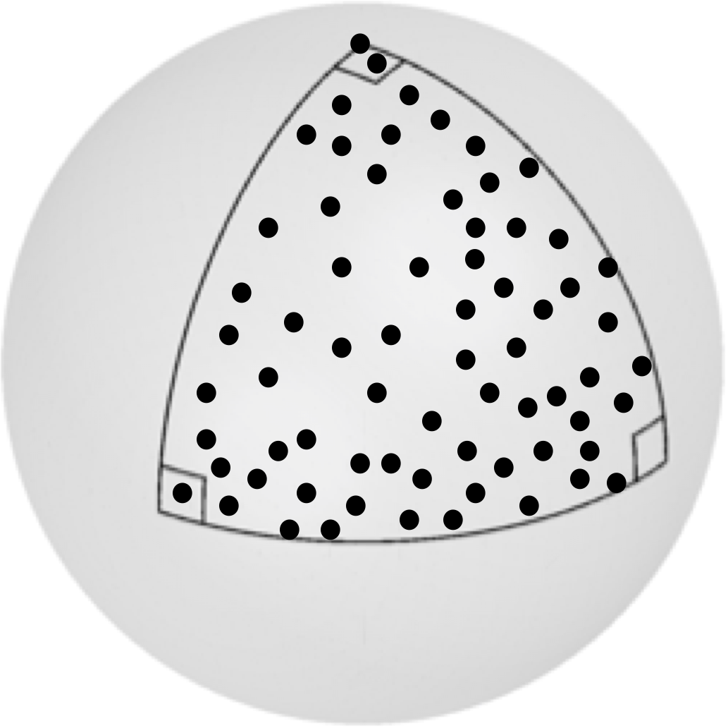
Figure 5. Unit sphere representing all directions in the object frame. A sufficiently large set of randomly selected points from the spherical triangle (or a larger one) contain the scheme (68) and satisfy the conditions in Theorem 4.1. Since $\epsilon={\mathcal{O}}(1/n)$ with a small constant, $|{\mathcal{T}}|$ is at least a large multiple of $n$.

In view of Theorem 3.1, 3.2 and 4.1, we have the following uniqueness results for 3D phase retrieval with a strong phase object.

Corollary 4.4.

Let ${\mathcal{T}}$ be a $\epsilon$-connected set of directions in Theorem 4.1 for a sufficiently small $\epsilon={\mathcal{O}}(1/n)$ satisfying (67). Consider the class of objects in $O_{n}$ with the maximum variation between two adjacent grid points less than $\pi/\kappa$.

(i) Under the setting of Theorem 3.1, the pairs of coded and uncoded diffraction patterns corresponding to $\mathbf{t}\in{\mathcal{T}}$ uniquely determine the strong phase object almost surely .

(ii) Under the setting of Corollary 3.3, the coded diffraction patterns corresponding to ${\mathcal{T}}$ uniquely determine the strong phase object almost surely.

4.1. The hybrid approximation

Let us sketch the extension of Theorem 4.1 to the hybrid approximation (6) with $q>1$ for which the phase unwrapping problem is finding conditions on ${\mathcal{T}}$ such that the relation

(80) $$\Big{(}1+{{\rm i}\kappa f_{\mathbf{t}}\over q}\Big{)}^{q}=\Big{(}1+{{\rm i}\kappa g_{\mathbf{t}}\over q}\Big{)}^{q},\quad\forall\mathbf{t}\in{\mathcal{T}},$$

for $f,g\in O_{n}$ implies $g=f$. Eq. (80) is equivalent to

(81) $$g_{\mathbf{t}}-\omega f_{\mathbf{t}}={q\over{\rm i}\kappa}(\omega-1)$$

where $\omega$ is a $q$-th root of unity.

By the above analysis an $\epsilon$-connected ${\mathcal{T}}$ with a sufficiently small $\epsilon={\mathcal{O}}(1/n)$ implies that $\omega$ in (81) is independent of $\mathbf{t}$. With a slight modification of the argument for Theorem 4.1, we arrive the conclusion that the right hand side of (81) is zero and hence $\omega=1$, implying $f=g$.

4.2. Tilt schemes for phase unwrapping

In this section, we consider a few examples as applications of Theorem 4.1 and Corollary 4.4.

4.2.1. Random tilt

We can satisfy condition (67) with overwhelming probability by randomly and independently selecting $n$ pairs of $(\alpha_{l},\beta_{l})$ that are distributed with probability density function bounded away from 0 and $\infty$ over any square contained in $[0,1]^{2}$ (see [6]).

In the case of (68) with $\alpha_{l},\beta_{l}\in[0,1)$, for instance, this random tilt series is distributed over the spherical rectangle of azimuth range $[0,\pi/4)$ and polar angle range $(\pi/4,\pi/2]$. We can enlarge the random sampling area from this spherical rectangle to the spherical triangle shown in Figure 5. If the sampling is sufficiently dense, then the whole scheme would include the direction $(0,1,\beta_{0})$, for some $\beta_{0}\in(0,1)$, and $\epsilon$-connect to $(0,0,1)$ (which is included by assumption),

More generally, the conditions of Theorem 4.1 are satisfied by any tilt series of sufficiently dense sampling from a spherical triangle with vertexes in three orthogonal directions (cf. Remark 4.3).

Random schemes arise naturally in single-particle imaging. On the other hand, deterministic tilt schemes are often employed in tomography.

4.2.2. Deterministic tilt

First, the single-axis tilting (with the conical angle $\pi/2$) is not covered by Theorem 4.1 and contains certain blindspot as exhibited in the proof, i.e. it can not completely resolve the ambiguities in phase unwrapping.

Second, certain combinations of (68), (69), (70), can be made $\epsilon$-connected (for sufficiently small $\epsilon$) in the following scheme:

$${\mathcal{T}} = \{(1,{l\over q},\alpha):l=0,\dots,q\}\cup\{({l\over q},1,\alpha):l=0,\dots,q\}$$

$$\cup\{(0,1,{l\over q}):l=0,\dots,q\}\cup\{(0,{l\over q},1):l=0,\dots,q\},\quad q\in\mathbb{N}$$

with a fixed $\alpha\in[0,1)$, where the first subset is from (68), the second and third from (69) and the fourth from (70). In the limit of $q\to\infty$, the scheme (4.2.2) has a continuous limit which can be illustrated more concretely in terms of the spherical polar coordinates as in the following example.

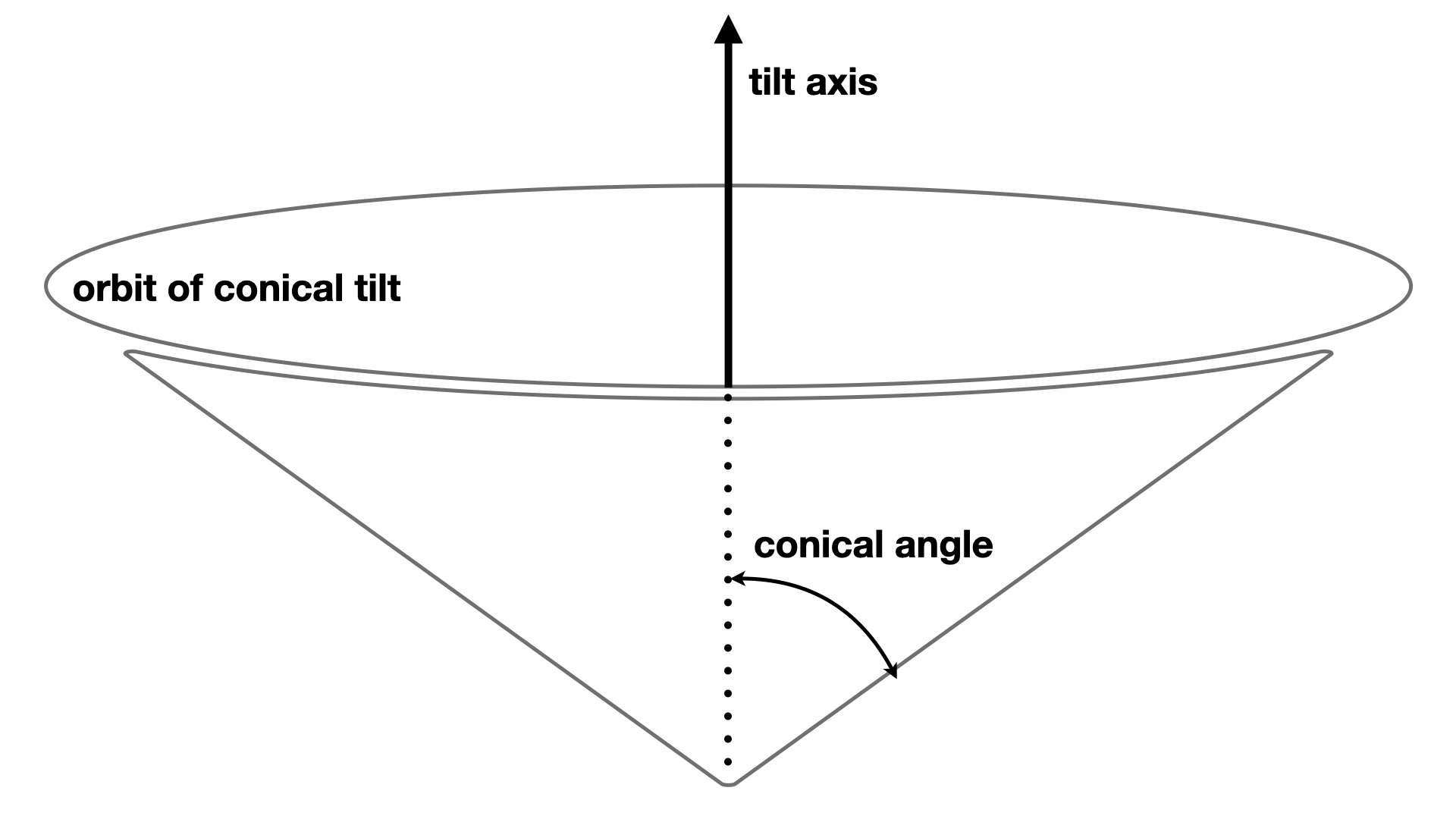
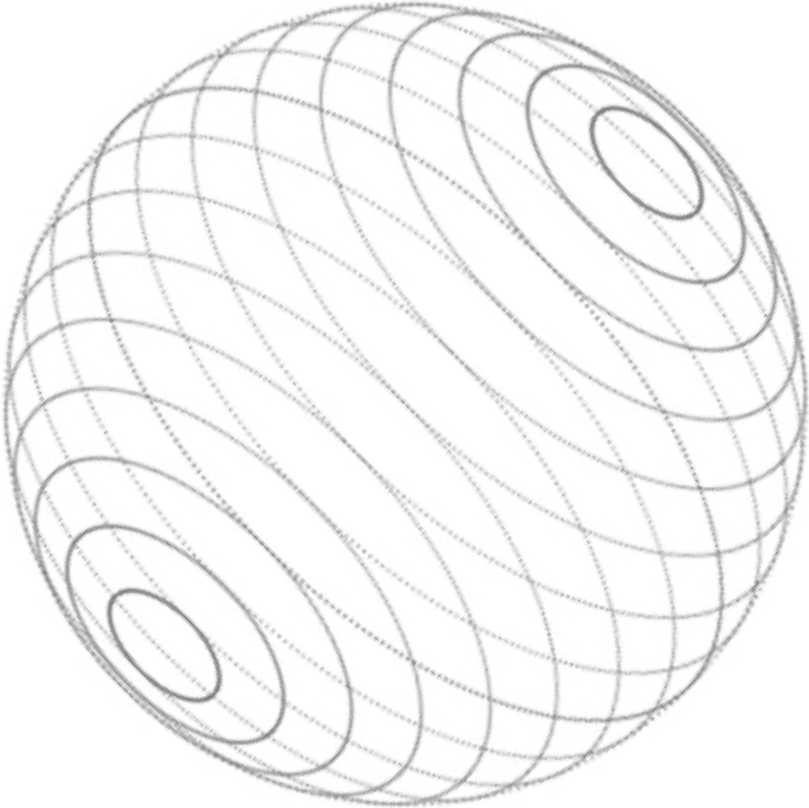
Figure 6. (a) Conical tilt geometry; (b) Conical tilt orbits of various conical angles about an axis of obliquity. A single-axis tilt orbit is a great circle, corresponding to a conical angle $\pi/2$, which can not uniquely unwrap phase.

Example 4.5.

The continuous limit of (4.2.2) consists of two circular arcs. The first arc, the limit of the first and second subsets in (4.2.2), going from $(1,0,\alpha)$ to $(1,1,\alpha)$ and to $(0,1,\alpha)$, is parametrized by the azimuthal angle $\phi_{z}\in[0,\pi/2],$ at the polar angle $\theta_{z}=\hbox{arc}\cot(\alpha)>\pi/4$ (since $\alpha\in[0,1)$) w.r.t. the polar axis $z$. The second arc, the limit of the third and fourth subsets in (4.2.2), going from $(0,1,\alpha)$ to $(0,1,1)$ and to $(0,0,1)$, is parametrized by the azimuthal angle $\phi_{x}\in[\arctan(\alpha),\pi/2],$ at the polar angle $\theta_{x}=\pi/2$ w.r.t. the polar axis $x$.

In other words, the continuous limit of (4.2.2) is an union of a conical tilting (the first arc) of range $\pi/2$ at the conical angle $\hbox{arc}\cot(\alpha)$ and an orthogonal single-axis tilting (the second arc) of range $\hbox{arc}\cot(\alpha)$.

For $\alpha=0$, the scheme is an orthogonal dual-axis tilting of a tilt range $\pi/2$ for each axis [78]. The total length of the orbit is $\pi$. $\square$.

Note that the total radiation dose is proportional to the number of projections, which is ${\mathcal{O}}(n)$ with a large constant (since $\epsilon={\mathcal{O}}(1/n)$ with a small constant), and, as $n\to\infty$, proportional to the orbit’s total length on the unit sphere.

More conveniently, instead of being split into a conical tilting and a single-axis tilting as in (4.2.2), the schemes in Theorem 4.1 can be implemented as a single conical tilting (Figure 6) which has a smooth circular orbit, instead of a broken one.

Example 4.6.

Let $(1,0,0)$ and $(0,0,1)$, respectively, be the start and the end of the orbit, with the midpoint $(0,1,0)$. Any three directions of the conical tilt uniquely determine the direction of the tilt axis, $(1,1,1),$ with the conical angle, $\arccos(1/\sqrt{3})\approx 54.7^{\circ},$ and the tilt range, $4\pi/3$. The total length of the orbit is ${4\pi\over 9}\sqrt{10-2\sqrt{3}}\approx 3.57$ which is slightly larger than the length $\pi$ in Example 4.5 for $\alpha=0$.

The conical tilt going through $(1,0,\alpha)$, $(0,1,\alpha)$ and $(0,0,1)$ can be similarly constructed. We leave the details to the interested reader. $\square$

5. Uniqueness with weak phase objects

In this section we show that for weak phase objects, much less restrictive schemes than those of Theorem 4.1 guarantee uniqueness of solution to 3D phase retrieval.

The following is the uniqueness result for discrete projection tomography.

Theorem 5.1.

Let ${\mathcal{T}}$ be any one of the following sets:

(83) $$\{(1,\alpha_{l},\beta_{l}):l=1,\dots,n\}$$

(84) $$\{(\alpha_{l},1,\beta_{l}):l=1,\dots,n\}$$

(85) $$\{(\alpha_{l},\beta_{l},1):l=1,\dots,n\}$$

under the condition (67). Suppose that $g_{\mathbf{t}}=e^{{\rm i}\theta_{0}}f_{\mathbf{t}},$ for some constant $\theta_{0}\in\mathbb{R}$, independent of $\mathbf{t}\in{\mathcal{T}}$. Then $g=e^{{\rm i}\theta_{0}}f$.

Remark 5.2.

Theorem 5.1 is the finite, discrete counterpart of the classical result that a compactly supported function is uniquely determined by the projections in any infinite set of directions ([45], proposition 7.8).

Proof.

To fix the idea, consider the case (85) for ${\mathcal{T}}$. By the discrete Fourier slice theorem, we have

(86) $$\widehat{g}(\xi,\eta,-\alpha_{l}\xi-\beta_{l}\eta) = e^{{\rm i}\theta_{0}}\widehat{f}(\xi,\eta,-\alpha_{l}\xi-\beta_{l}\eta),\quad l=1,\dots,n,\quad\xi,\eta\in\mathbb{Z}.$$

In other words, for each $\xi,\eta\in\mathbb{Z},$ the corresponding partial Fourier transforms defined in (75) satisfy

(87) $$\sum_{m\in\mathbb{Z}_{n}}(\widehat{g}_{\xi\eta}(m)-e^{{\rm i}\theta_{0}}\widehat{f}_{\xi\eta}(m))e^{-{\rm i}2\pi m(-\alpha_{l}\xi-\beta_{l}\eta)/p}=0,\quad l=1,...,n$$

in terms of the notation for partial Fourier transforms in the proof of Theorem 4.1. For each $\xi,\eta,$ (87) is a Vandermonde system which is nonsingular if and only if (67) holds. This implies that

$$\widehat{g}_{\xi\eta}(m)=e^{{\rm i}\theta_{0}}\widehat{f}_{\xi\eta}(m),\quad m\in\mathbb{Z}_{p},\quad\forall\xi,\eta\in\mathbb{Z}.$$

Therefore, $g=e^{{\rm i}\theta_{0}}f$ as asserted. ∎

It may be interesting to compare Theorem 5.1 with Crowther’s rough estimate

(88) $$N={\pi\over 2}n$$

for the number $N$ of projections needed for projection tomography with a single-axis tilting of tilt range $\pi$ ([55], eq. (8.3)).

We have the following uniqueness results for 3D phase retrieval with a weak phase object.

Corollary 5.3.

Let ${\mathcal{T}}$ be any one of the direction sets in Theorem 5.1.

• Under the setting of Theorem 3.4, the $n$ pairs of coded and uncoded diffraction patterns corresponding to ${\mathcal{T}}$ uniquely determine the weak phase object almost surely.

• Under the setting of Corollary 3.8, the $n$ coded diffraction patterns corresponding to ${\mathcal{T}}$ uniquely determine the weak phase object with high probability (for $n\gg 1$).

In contrast to Corollary 5.3 (ii), the setting of Corollary 3.6 requires an extra coded diffraction pattern to remove the isotropy ambiguity.

Theorem 5.4.

[26] Let ${\mathcal{T}}$ be any one of the following direction sets

(89) $$\{(1,\alpha_{l},\beta_{l}):l=1,\dots,n\}\cup\{(0,\alpha_{0},\beta_{0})\}$$

(90) $$\{(\alpha_{l},1,\beta_{l}):l=1,\dots,n\}\cup\{(\alpha_{0},0,\beta_{0})\}$$

(91) $$\{(\alpha_{l},\beta_{l},1):l=1,\dots,n\}\cup\{(\alpha_{0},\beta_{0},0)\}$$

under the condition (67) and $(\alpha_{0},\beta_{0})\neq(0,0)$. Then in the setting of Corollary 3.6, $g=e^{{\rm i}\theta_{0}}f$ for some constant $\theta_{0}\in\mathbb{R}$ almost surely.

Proof.

To rule out the second alternative in Corollary 3.6 that $f^{*}_{\mathbf{t}}=f^{*}_{\mathbf{t}^{\prime}},\forall\mathbf{t},\mathbf{t}^{\prime}\in{\mathcal{T}},$ define $h_{\mathbf{t}}:=f^{*}_{\mathbf{t}}$ which is independent of $\mathbf{t}\in{\mathcal{T}}$. Now applying the analysis in the proof of Theorem 4.1 to this $h_{\mathbf{t}}$ for the scheme, e.g. (89). The argument up to (78) leads to the conclusion that the projection of $h$ in the direction of $(0,\alpha_{0},\beta_{0}),$ with $\alpha_{0}\neq 0,$ is part of a line segment and hence $h_{\mathbf{t}}$ is a line object for all $\mathbf{t}\in{\mathcal{T}}$. This violates the assumption in Corollary 3.6 that no projection is part of a line. This implies that the first alternative of Corollary 3.6 holds, i.e. ${g_{\mathbf{t}}}=e^{{\rm i}\theta_{0}}f_{\mathbf{t}},\quad\forall\mathbf{t}\in{\mathcal{T}}.$ ∎

6. Noise robustness

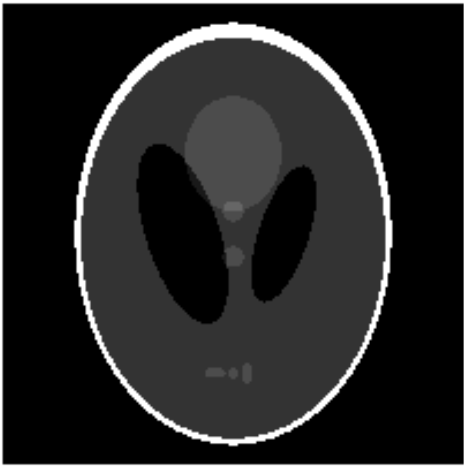
(a) 2D image

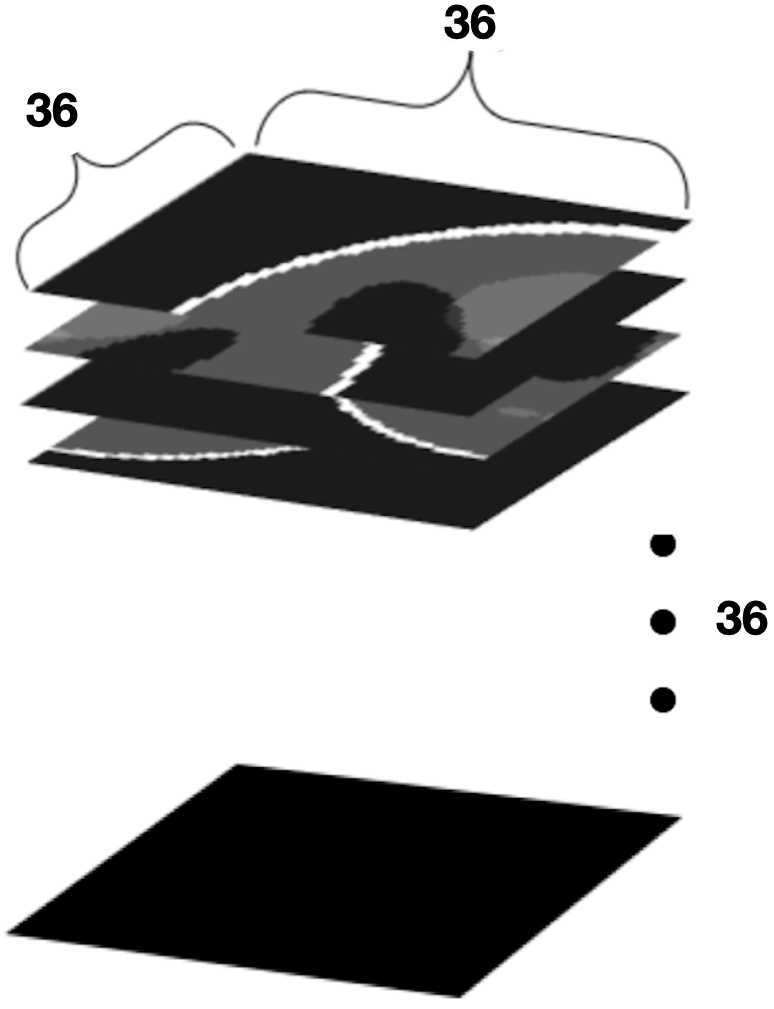
(b) 3D representation

Figure 7. $216\times 216$ image sliced and stacked unto a $36\times 36\times 36$ object.

Let us turn to the shot noise issue not addressed by the preceding uniqueness results. At present, there are few theoretical results on noise robustness in phase retrieval except for simplified models [24].

In practice, noise stability has as much to do with the reconstruction method as the information content of the given dataset. However, assessing and optimizing algorithms for 3D reconstruction from a large number of snapshots is by itself a challenging ongoing task [77]. Herein, we limit ourselves to testing the noise robustness of alternating projection [15] (also known as Error-Reduction [33] or Gerchberg-Saxton [38] algorithm) in the case of weak phase objects to avoid the phase unwrapping problem altogether.

First the ideal, noiseless detection process with a weak-phase object can be written as $b^{2}=|{\mathcal{A}}f_{*}|^{2}$ in terms of a measurement matrix ${\mathcal{A}}$ representing the process $f\stackrel{{\scriptstyle{\mathcal{A}}}}{{\longrightarrow}}(\widehat{f}_{\mathbf{t}}\star\widehat{\mu})_{\mathbf{t}\in{\mathcal{T}}}.$

In alternating projection (AP), the reconstruction procedure alternates between the object-constraint projection ${\mathcal{P}}_{1}={\mathcal{A}}{\mathcal{A}}^{\dagger}$, where $A^{\dagger}$ is the pseudo-inverse of ${\mathcal{A}}$, and the data-constrained projection ${\mathcal{P}}_{2}h=b\odot\hbox{sgn}(h),$ where $\hbox{sgn}(h)$ is the phase factor vector of $h$. AP can be represented as $({\mathcal{P}}_{1}{\mathcal{P}}_{2})^{k}f_{0},k\in\mathbb{N},$ with a random initialization $f_{0}$ [15].

Notably AP is the gradient descent with unit step size for

(92) $$\min_{u}\|b-|{\mathcal{A}}u|\|$$

which is a simplified asymptotic surrogate for maximizing the Poisson log-likelihood function [31].

6.1. Noise-to-signal ratio (NSR)

To introduce the Poisson noise into our set-up, let $\widetilde{b}^{2}$ be the Poisson random vectors with the mean $sb^{2}$ where the adjustable scale factor $s>0$ represents the overall strength of object-radiation interaction.

The noise level is measured by the noise-to-signal ratio (NSR)

(93) $$\hbox{NSR}:={\hbox{\# total average non-signal photons}\over\hbox{ \# total signal photons}}.$$

Let $z=(z_{j}):=\widetilde{b}^{2}-sb^{2}$. The total average noise photon count is proportional to

(94) $$\sum_{j}\mathbb{E}|z_{j}| \sum_{j}\sqrt{\mathbb{E}|z_{j}|^{2}}=\Big{\|}\sqrt{\hbox{var}(\widetilde{b}^{2})}\Big{\|}_{1}$$ or more conveniently

where $\|\cdot\|_{1}$ denotes the L1-norm. In other words, the NSR (93) can be conveniently calculated as

(95) NSR $$:= {\Big{\|}\sqrt{\hbox{var}(\widetilde{b}^{2})}\Big{\|}_{1}\over\|\mathbb{E}(\widetilde{b}^{2})\|_{1}}={\|{b}\|_{1}\over\sqrt{s}\|b^{2}\|_{1}}.$$

6.2. Numerical results

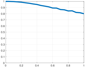
(a) $R$ vs NSR $\in$ (0,1)

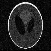
(b) NSR=0.5

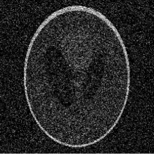
(c) NSR=1

Figure 8. Randomly initialized AP reconstruction: (a) correlation vs NSR; (b) flattened reconstruction at NSR =0.5 & (c) NSR = 1.

In our simulations, we take the mask phase $\phi$ to be an independent uniform random variable over $[0,2\pi)$ for each pixel.

We construct the real-valued 3D object from the $216\times 216$ phantom (Fig. 7 (a)) by partitioning the phantom into 36 pieces, each of which is $36\times 36$ and stacking them into a $36\times 36\times 36$ cube (Fig. 7(b)). This is to facilitate the “eye-ball” metric for qualitative evaluation of the reconstruction. For a quantitative metric, we use the absolute correlation

$$R(f,f_{*}):={|\bar{f}\cdot f_{*}|\over\|f\|\|f_{*}\|}$$

between the true object $f_{*}$ and the reconstruction $f$.

To avoid the missing cone problem in tomography [34], we use the random tilt scheme comprised of the union of (89), (90) and (91), in the form

$${\mathcal{T}} = \{\mathbf{t}_{i}=(1,\alpha_{i},\beta_{i})\}_{i=1}^{n}\cup\{\mathbf{t}_{i}=(\alpha_{i},1,\beta_{i})\}_{i=1+n}^{2n}\cup\{\mathbf{t}_{i}=(\alpha_{i},\beta_{i},1)\}_{i=2n+1}^{3n}$$

$$\hbox{with $\alpha_{i},\beta_{i},i=1,\cdots,3n,$ randomly chosen from $(-1,1)$}.$$

which has a significantly larger range of possibility than that portrayed in Figure 5. To reduce the burden of computer memory, we do not oversample the Fourier transform in our numerical simulation, i.e. $b,\widetilde{b}\in\mathbb{R}^{mp^{2}}$ with $m=3n$. Consequently, the total amount of measurement data is about $3/4$ of that assumed in Theorem 5.1.

To take advantage of the prior information that the object is real-valued, we use ${\mathcal{P}}_{1}={\mathcal{A}}\Re{\mathcal{A}}^{\dagger}$ in AP reconstruction where $\Re$ is the projection unto the real-part. As shown in Figure 8, randomly initialized AP with the data set $\eqref{tset}$ is capable of handling high levels of noise.

The convergence rate, however, can be further improved by using more sophisticated algorithms (see [31], [30] and references therein). When applicable, various sparsity priors can enhance numerical reconstruction’s robustness to noise [51, 84, 70, 8, 83]. Finally, the coded aperture itself needs not be known in advance and can be simultaneously calibrated by effective algorithms with a sufficiently large set ${\mathcal{T}}$ [27, 29].

7. Discussion and extension

While our results are primarily aimed at diffraction tomography with known orientations, the idea of reducing phase retrieval to (phase) projection tomography by pair-wise measurements (Theorem 3.1, 3.2, 3.4 and 3.5) have potential applications to single-particle imaging which typically is subject to higher level of measurement uncertainties.

Specifically the proposed measurement schemes embodied in Figure 3 enable the reconstruction of (phase) projections in various unknown orientations $\mathbf{t}$. Since it is easier to mitigate measurement uncertainties with projection data than diffraction data, the measurement uncertainties in X-ray and electron experiments with small-sized objects such as nano-crystals and macromolecules may be handled by projection-based methods (see [16, 68, 13, 75, 69]).

For example, for a weak phase object, classification and alignment can then be carried out with single-particle cryo-EM methods such as the common-line methods [21, 90, 88], the maximum-likelihood methods [87, 66] and the Bayesian methods [81, 82] based on projection data instead of diffraction patterns [50, 85, 64, 35, 40].

For a strong phase object, however, there remain several hurdles. The foremost is developing effective numerical algorithms for 3D phase unwrapping which is not as well studied as 2D phase unwrapping [39].

After the alignment of the phase projections, it is tempting to apply the 2D phase unwrapping methods and try to recover the projection from the phase projection in each direction. The projection in each direction, however, usually violate the 2D Itoh condition even when the 3D Itch condition holds. If the 2D Itoh condition fails to hold at a large number of pixels, then 2D phase unwrapping becomes more complicated, requiring additional prior information. Moreover, the unwrapped phases for different directions must be consistent with one another. Hence the 3D phase unwrapping problem should be approached with all phase projections together instead of one direction at a time.

A similar approach called ptychographic tomography has been proposed and studied numerically [23, 42, 48, 43, 62]. The difference from the present work is that in ptychography, instead of simultaneous pairwise measurements of the whole object, multiple significantly overlapped diffraction patterns are measured in each direction by sequentially shifting the aperture over different parts of the object. As a consequence, ptychographic tomography is limited to sizable objects capable of sustaining multiple intense illuminations and hence not suitable for, e.g. single particle imaging.

Appendix A Proof of Theorem 3.1

The following result is our basic tool.

Lemma A.1.

[25] Let $\mu$ be the phase mask (i.e. $\mu({\mathbf{n}})=\exp[{\rm i}\phi({\mathbf{n}})],\phi({\mathbf{n}})\in\mathbb{R},\forall{\mathbf{n}}$) with independent, continuous random variables $\phi({\mathbf{n}})\in\mathbb{R}$. If $e^{{\rm i}\kappa g_{\mathbf{t}}}\odot\nu$ produces the same diffraction pattern as $e^{{\rm i}\kappa f_{\mathbf{t}}}\odot\mu$, then for some $\mathbf{m}_{\mathbf{t}}\in\mathbb{Z}^{2},\theta_{\mathbf{t}}\in\mathbb{R}$

$$e^{{\rm i}\kappa g_{\mathbf{t}}({\mathbf{n}})}\nu({\mathbf{n}}) = \hbox{\rm either}\quad e^{{\rm i}\theta_{\mathbf{t}}}e^{{\rm i}\kappa f_{\mathbf{t}}({\mathbf{n}}+\mathbf{m}_{\mathbf{t}})}\mu({\mathbf{n}}+\mathbf{m}_{\mathbf{t}})$$

$$\quad\hbox{\rm or}\quad e^{{\rm i}\theta_{\mathbf{t}}}e^{-{\rm i}\kappa\overline{f_{\mathbf{t}}(-{\mathbf{n}}+\mathbf{m}_{\mathbf{t}})}}\overline{\mu(-{\mathbf{n}}+\mathbf{m}_{\mathbf{t}})}$$

for all ${\mathbf{n}}$.

Lemma A.1 is a special case of the more general result in [25] which is not limited to phase masks. Note that the statement holds for any real-valued continuous random variable $\phi({\mathbf{n}})$. By more advanced techniques from algebraic geometry and probability, one can relax the conditions of continuity and independence on $\phi({\mathbf{n}})$.

After taking logarithm, (A.1) becomes

$$\kappa g_{\mathbf{t}}({\mathbf{n}})-{\rm i}\ln\nu({\mathbf{n}}) = \hbox{\rm either}\quad\theta_{\mathbf{t}}+\kappa f_{\mathbf{t}}({\mathbf{n}}+\mathbf{m}_{\mathbf{t}})-{\rm i}\ln\mu({\mathbf{n}}+\mathbf{m}_{\mathbf{t}})$$

$$\quad\hbox{or}\quad\theta_{\mathbf{t}}-\kappa\overline{f_{\mathbf{t}}(-{\mathbf{n}}+\mathbf{m}_{\mathbf{t}})}-{\rm i}\ln\overline{\mu(-{\mathbf{n}}+\mathbf{m}_{\mathbf{t}})}$$

modulo $2\pi.$

If $\mu$ is completely known, i.e. $\nu=\mu$, then (A) becomes

$$\kappa g_{\mathbf{t}}({\mathbf{n}})-{\rm i}\ln\mu({\mathbf{n}}) = \hbox{\rm either}\quad\theta_{\mathbf{t}}+\kappa f_{\mathbf{t}}({\mathbf{n}}+\mathbf{m}_{\mathbf{t}})-{\rm i}\ln\mu({\mathbf{n}}+\mathbf{m}_{\mathbf{t}})$$

$$\quad\hbox{\rm or}\quad\theta_{\mathbf{t}}-\kappa\overline{f_{\mathbf{t}}(-{\mathbf{n}}+\mathbf{m}_{\mathbf{t}})}-{\rm i}\ln\overline{\mu(-{\mathbf{n}}+\mathbf{m}_{\mathbf{t}})}$$

modulo $2\pi$.

Since both diffraction patterns are from the same snapshot, we can reset the object frame so that ${\mathbf{l}}_{\mathbf{t}}=0$.

Suppose the first alternative in (A) holds with $\mathbf{m}_{\mathbf{t}}\not=0$. By (44), $e^{{\rm i}\kappa f_{\mathbf{t}}}$ and $e^{{\rm i}\kappa g_{\mathbf{t}}}$ have the same autocorrelation function and hence

$$\sum_{\mathbf{n}}e^{{\rm i}\kappa(f_{\mathbf{t}}({\mathbf{n}}+{\mathbf{k}})-\overline{f_{\mathbf{t}}({\mathbf{n}})})} = \sum_{\mathbf{n}}e^{{\rm i}\kappa(f_{\mathbf{t}}({\mathbf{n}}+\mathbf{m}_{\mathbf{t}}+{\mathbf{k}})-\overline{f_{\mathbf{t}}({\mathbf{n}}+\mathbf{m}_{\mathbf{t}})})}e^{{\rm i}(\phi({\mathbf{n}}+\mathbf{m}_{\mathbf{t}}+{\mathbf{k}})-\phi({\mathbf{n}}+{\mathbf{k}}))}e^{-{\rm i}(\phi({\mathbf{n}}+\mathbf{m}_{\mathbf{t}})-\phi({\mathbf{n}}))}$$

for all ${\mathbf{k}}$, or equivalently

$$\sum_{\mathbf{n}}e^{{\rm i}\kappa(f_{\mathbf{t}}({\mathbf{n}}+\mathbf{m}_{\mathbf{t}}+{\mathbf{k}})-\overline{f_{\mathbf{t}}({\mathbf{n}}+\mathbf{m}_{\mathbf{t}})})}$$

$$= \sum_{\mathbf{n}}e^{{\rm i}\kappa(f_{\mathbf{t}}({\mathbf{n}}+\mathbf{m}_{\mathbf{t}}+{\mathbf{k}})-\overline{f_{\mathbf{t}}({\mathbf{n}}+\mathbf{m}_{\mathbf{t}})})}e^{{\rm i}(\phi({\mathbf{n}}+\mathbf{m}_{\mathbf{t}}+{\mathbf{k}})-\phi({\mathbf{n}}+\mathbf{m}_{\mathbf{t}})-\phi({\mathbf{n}}+{\mathbf{k}})+\phi({\mathbf{n}}))}$$

by change of index, ${\mathbf{n}}\to{\mathbf{n}}+\mathbf{m}_{\mathbf{t}}$, on the left hand side of equation. Define

$$\Delta_{\mathbf{k}}f_{\mathbf{t}}({\mathbf{n}}+\mathbf{m}_{\mathbf{t}}):=f_{\mathbf{t}}({\mathbf{n}}+\mathbf{m}_{\mathbf{t}}+{\mathbf{k}})-\overline{f_{\mathbf{t}}({\mathbf{n}}+\mathbf{m}_{\mathbf{t}})}$$

and rewrite (A) as

(101) $$0 = \sum_{{\mathbf{n}}}\left[e^{{\rm i}(\phi({\mathbf{n}}+\mathbf{m}_{\mathbf{t}}+{\mathbf{k}})-\phi({\mathbf{n}}+\mathbf{m}_{\mathbf{t}})-\phi({\mathbf{n}}+{\mathbf{k}})+\phi({\mathbf{n}}))}-1\right]e^{{\rm i}\kappa\Delta_{\mathbf{k}}f_{\mathbf{t}}({\mathbf{n}}+\mathbf{m}_{\mathbf{t}})},$$

for all ${\mathbf{k}}$. We want to show that the probability of the event (101) is zero.

Let us consider those summands in (101), for any fixed ${\mathbf{k}}$, that share a common $\phi({\mathbf{l}})$, for any fixed ${\mathbf{l}}$, in the expression. Clearly, there are at most four such terms:

$$\left[e^{{\rm i}(\phi({\mathbf{l}})-\phi({\mathbf{l}}-{\mathbf{k}})-\phi({\mathbf{l}}-\mathbf{m}_{\mathbf{t}})+\phi({\mathbf{l}}-{\mathbf{k}}-\mathbf{m}_{\mathbf{t}}))}-1\right]e^{{\rm i}\kappa\Delta_{\mathbf{k}}f_{\mathbf{t}}({\mathbf{l}}-{\mathbf{k}})}$$

$$+ \left[e^{{\rm i}(\phi({\mathbf{l}}+{\mathbf{k}})-\phi({\mathbf{l}})-\phi({\mathbf{l}}+{\mathbf{k}}-\mathbf{m}_{\mathbf{t}})+\phi({\mathbf{l}}-\mathbf{m}_{\mathbf{t}}))}-1\right]e^{{\rm i}\kappa\Delta_{\mathbf{k}}f_{\mathbf{t}}({\mathbf{l}})}$$

$$+ \left[e^{{\rm i}(\phi({\mathbf{l}}+\mathbf{m}_{\mathbf{t}})-\phi({\mathbf{l}}-{\mathbf{k}}+\mathbf{m}_{\mathbf{t}})-\phi({\mathbf{l}})+\phi({\mathbf{l}}-{\mathbf{k}}))}-1\right]e^{{\rm i}\kappa\Delta_{\mathbf{k}}f_{\mathbf{t}}({\mathbf{l}}-{\mathbf{k}}+\mathbf{m}_{\mathbf{t}})}$$

$$+ \left[e^{{\rm i}(\phi({\mathbf{l}}+{\mathbf{k}}+\mathbf{m}_{\mathbf{t}})-\phi({\mathbf{l}}+\mathbf{m}_{\mathbf{t}})-\phi({\mathbf{l}}+{\mathbf{k}})+\phi({\mathbf{l}}))}-1\right]e^{{\rm i}\kappa\Delta_{\mathbf{k}}f_{\mathbf{t}}({\mathbf{l}}+\mathbf{m}_{\mathbf{t}})}.$$

Since the continuous random variable $\phi({\mathbf{l}})$ does not appear in other summands and hence is independent of them, (101) implies that (A) (and the rest of (101)) must vanish almost surely.

For ${\mathbf{k}}$ that are linearly independent of $\mathbf{m}_{\mathbf{t}}$, the four independent random variables

(103) $$\phi({\mathbf{l}}-{\mathbf{k}}-\mathbf{m}_{\mathbf{t}}),\quad\phi({\mathbf{l}}+{\mathbf{k}}-\mathbf{m}_{\mathbf{t}}),\quad\phi({\mathbf{l}}-{\mathbf{k}}+\mathbf{m}_{\mathbf{t}}),\quad\phi({\mathbf{l}}+{\mathbf{k}}+\mathbf{m}_{\mathbf{t}})$$

appear separately in exactly one summand in (A). Consequently, (A) (and hence (101)) almost surely does not vanishes for ${\mathbf{k}}$ that are linearly independent of $\mathbf{m}_{\mathbf{t}}$.

On the other hand, if ${\mathbf{k}}$ is parallel to $\mathbf{m}_{\mathbf{t}}\neq 0$, then for any

$${\mathbf{k}}\not\in\{\pm\mathbf{m}_{\mathbf{t}},\pm{1\over 2}\mathbf{m}_{\mathbf{t}},\pm 2\mathbf{m}_{\mathbf{t}}\}$$

the four terms in (103) appear separately in exactly one summand in (A). Consequently, (A) almost surely does not vanishes.

Thus whenever the first alternative in (A) holds true, we have $\mathbf{m}_{\mathbf{t}}=0$ and $e^{{\rm i}\kappa g_{\mathbf{t}}}=e^{{\rm i}\theta_{\mathbf{t}}}e^{{\rm i}\kappa f_{\mathbf{t}}}$ for some constant $\theta_{\mathbf{t}}$ independent of the grid point.

Next, we show that the second alternative in (A.1) is false. By (44), we have

$$\sum_{\mathbf{n}}e^{{\rm i}\kappa(f_{\mathbf{t}}({\mathbf{n}}+{\mathbf{k}})-\overline{f_{\mathbf{t}}({\mathbf{n}})})}$$

$$= \sum_{\mathbf{n}}e^{-{\rm i}\kappa(\overline{f_{\mathbf{t}}(-{\mathbf{n}}+\mathbf{m}_{\mathbf{t}}+{\mathbf{k}})}-f_{\mathbf{t}}(-{\mathbf{n}}+\mathbf{m}_{\mathbf{t}}))}e^{-{\rm i}(\phi(-{\mathbf{n}}+\mathbf{m}_{\mathbf{t}}+{\mathbf{k}})+\phi({\mathbf{n}}+{\mathbf{k}}))}e^{{\rm i}(\phi(-{\mathbf{n}}+\mathbf{m}_{\mathbf{t}})+\phi({\mathbf{n}}))}$$

for all ${\mathbf{k}}$, or equivalently

$$\sum_{\mathbf{n}}e^{{\rm i}\kappa(f_{\mathbf{t}}({\mathbf{n}}+\mathbf{m}_{\mathbf{t}}+{\mathbf{k}})-\overline{f_{\mathbf{t}}({\mathbf{n}}+\mathbf{m}_{\mathbf{t}})})}$$

$$= \sum_{\mathbf{n}}e^{-{\rm i}\kappa(\overline{f_{\mathbf{t}}(-{\mathbf{n}}+\mathbf{m}_{\mathbf{t}}+{\mathbf{k}})}-f_{\mathbf{t}}(-{\mathbf{n}}+\mathbf{m}_{\mathbf{t}}))}e^{-{\rm i}(\phi(-{\mathbf{n}}+\mathbf{m}_{\mathbf{t}}+{\mathbf{k}})+\phi({\mathbf{n}}+{\mathbf{k}}))}e^{{\rm i}(\phi(-{\mathbf{n}}+\mathbf{m}_{\mathbf{t}})+\phi({\mathbf{n}}))}$$

by change of index, ${\mathbf{n}}\to-{\mathbf{n}}+\mathbf{m}_{\mathbf{t}}$, on the left hand side of equation. With

$$\Delta_{\mathbf{k}}\overline{f_{\mathbf{t}}(-{\mathbf{n}}+\mathbf{m}_{\mathbf{t}})}:=\overline{f_{\mathbf{t}}(-{\mathbf{n}}+\mathbf{m}_{\mathbf{t}}+{\mathbf{k}})}-f_{\mathbf{t}}(-{\mathbf{n}}+\mathbf{m}_{\mathbf{t}})$$

we rewrite (A) as

(105) $$0 = \sum_{\mathbf{n}}\left[e^{{\rm i}(-\phi(-{\mathbf{n}}+\mathbf{m}_{\mathbf{t}}+{\mathbf{k}})+\phi(-{\mathbf{n}}+\mathbf{m}_{\mathbf{t}})-\phi({\mathbf{n}}+{\mathbf{k}})+\phi({\mathbf{n}}))}-1\right]e^{-{\rm i}\kappa\Delta_{\mathbf{k}}\overline{f_{\mathbf{t}}(-{\mathbf{n}}+\mathbf{m}_{\mathbf{t}})}}$$

for all ${\mathbf{k}}$. We want to show that the right hand side of (105) almost surely does not vanish for any ${\mathbf{k}}$.

As before, consider those summands in (105), for any fixed ${\mathbf{k}}$, that share a common $\phi({\mathbf{l}})$, for any fixed ${\mathbf{l}}$, in the expression. Clearly, there are at most four such terms:

(106) $$\left[e^{{\rm i}(-\phi({\mathbf{l}})+\phi({\mathbf{l}}+{\mathbf{k}})-\phi(-{\mathbf{l}}+\mathbf{m}_{\mathbf{t}})+\phi(-{\mathbf{l}}-{\mathbf{k}}+\mathbf{m}_{\mathbf{t}}))}-1\right]e^{-{\rm i}\kappa\Delta_{\mathbf{k}}\overline{f_{\mathbf{t}}({\mathbf{l}})}}$$

$$+\left[e^{{\rm i}(-\phi({\mathbf{l}}-{\mathbf{k}})+\phi({\mathbf{l}})-\phi(-{\mathbf{l}}+{\mathbf{k}}+\mathbf{m}_{\mathbf{t}})+\phi(-{\mathbf{l}}+\mathbf{m}_{\mathbf{t}}))}-1\right]e^{-{\rm i}\kappa\Delta_{\mathbf{k}}\overline{f_{\mathbf{t}}({\mathbf{l}}-{\mathbf{k}})}}$$

$$+\left[e^{{\rm i}(-\phi(-{\mathbf{l}}+\mathbf{m}_{\mathbf{t}})+\phi(-{\mathbf{l}}+{\mathbf{k}}+\mathbf{m}_{\mathbf{t}})-\phi({\mathbf{l}})+\phi({\mathbf{l}}-{\mathbf{k}}))}-1\right]e^{-{\rm i}\kappa\Delta_{\mathbf{k}}\overline{f_{\mathbf{t}}(-{\mathbf{l}}+\mathbf{m}_{\mathbf{t}})}}$$

$$+\left[e^{{\rm i}(-\phi(-{\mathbf{l}}-{\mathbf{k}}+\mathbf{m}_{\mathbf{t}})+\phi(-{\mathbf{l}}+\mathbf{m}_{\mathbf{t}})-\phi({\mathbf{l}}+{\mathbf{k}})+\phi({\mathbf{l}}))}-1\right]e^{-{\rm i}\kappa\Delta_{\mathbf{k}}\overline{f_{\mathbf{t}}(-{\mathbf{l}}-{\mathbf{k}}+\mathbf{m}_{\mathbf{t}})}}$$

With $\phi({\mathbf{l}})$ appearing in no other terms, (105) implies that (106) must vanish almost surely.

Some observations are in order. First, both $\phi({\mathbf{l}})$ and $\phi(-{\mathbf{l}}+\mathbf{m}_{\mathbf{t}})$ appear exactly once in each summand in (134). Second, the following pairings of the other phases

$$\{\phi({\mathbf{l}}+{\mathbf{k}}),\phi(-{\mathbf{l}}-{\mathbf{k}}+\mathbf{m}_{\mathbf{t}})\},\quad\{\phi({\mathbf{l}}-{\mathbf{k}}),\phi(-{\mathbf{l}}+{\mathbf{k}}+\mathbf{m}_{\mathbf{t}})\}$$

also appear exactly twice in (134). As long as ${\mathbf{k}}\not=0$ and $2{\mathbf{l}}\neq\mathbf{m}_{\mathbf{t}}$, these two pairs are not identical and hence

$$0 = \left[e^{{\rm i}(-\phi({\mathbf{l}})+\phi({\mathbf{l}}+{\mathbf{k}})-\phi(-{\mathbf{l}}+\mathbf{m}_{\mathbf{t}})+\phi(-{\mathbf{l}}-{\mathbf{k}}+\mathbf{m}_{\mathbf{t}}))}-1\right]e^{-{\rm i}\kappa\Delta_{\mathbf{k}}\overline{f_{\mathbf{t}}({\mathbf{l}})}}$$

$$+\overline{\left[e^{{\rm i}(\phi(-{\mathbf{l}}-{\mathbf{k}}+\mathbf{m}_{\mathbf{t}})-\phi(-{\mathbf{l}}+\mathbf{m}_{\mathbf{t}})+\phi({\mathbf{l}}+{\mathbf{k}})-\phi({\mathbf{l}}))}-1\right]}e^{-{\rm i}\kappa\Delta_{\mathbf{k}}\overline{f_{\mathbf{t}}(-{\mathbf{l}}-{\mathbf{k}}+\mathbf{m}_{\mathbf{t}})}}$$

$$0 = \left[e^{{\rm i}(-\phi({\mathbf{l}}-{\mathbf{k}})+\phi({\mathbf{l}})-\phi(-{\mathbf{l}}+{\mathbf{k}}+\mathbf{m}_{\mathbf{t}})+\phi(-{\mathbf{l}}+\mathbf{m}_{\mathbf{t}}))}-1\right]e^{-{\rm i}\kappa\Delta_{\mathbf{k}}\overline{f_{\mathbf{t}}({\mathbf{l}}-{\mathbf{k}})}}$$

$$+\overline{\left[e^{{\rm i}(\phi(-{\mathbf{l}}+\mathbf{m}_{\mathbf{t}})-\phi(-{\mathbf{l}}+{\mathbf{k}}+\mathbf{m}_{\mathbf{t}})+\phi({\mathbf{l}})-\phi({\mathbf{l}}-{\mathbf{k}}))}-1\right]}e^{-{\rm i}\kappa\Delta_{\mathbf{k}}\overline{f_{\mathbf{t}}(-{\mathbf{l}}+\mathbf{m}_{\mathbf{t}})}}$$

both of which are almost surely false because the two factors

$$\left[e^{{\rm i}(-\phi({\mathbf{l}})+\phi({\mathbf{l}}+{\mathbf{k}})-\phi(-{\mathbf{l}}+\mathbf{m}_{\mathbf{t}})+\phi(-{\mathbf{l}}-{\mathbf{k}}+\mathbf{m}_{\mathbf{t}}))}-1\right],\quad\left[e^{{\rm i}(-\phi({\mathbf{l}}-{\mathbf{k}})+\phi({\mathbf{l}})-\phi(-{\mathbf{l}}+{\mathbf{k}}+\mathbf{m}_{\mathbf{t}})+\phi(-{\mathbf{l}}+\mathbf{m}_{\mathbf{t}}))}-1\right]$$

differ with their complex conjugates in a random manner independently from $f_{\mathbf{t}}$.

Therefore, the second alternative in (A) almost surely does not hold true.

In summary, the first alternative in (A) holds with $\mathbf{m}_{\mathbf{t}}=0$, namely

$$\kappa g_{\mathbf{t}}({\mathbf{n}}) = \theta_{\mathbf{t}}+\kappa f_{\mathbf{t}}({\mathbf{n}})\quad\mod 2\pi$$

almost surely.

The actual support of the projections (21)-(23) for $0\leq\alpha,\beta\leq 1$ and odd integer $n$, for example, is contained in

(108) $$\bigcup_{i\in\mathbb{Z}_{n}}(\mathbb{Z}_{n}-\lfloor\alpha i\rfloor)\times(\mathbb{Z}_{n}-\lfloor\beta i\rfloor)$$

where $\lfloor\cdot\rfloor$ denotes the floor function. In turn, the set in (108) is a subset of

(109) $$\left\{\bigcup_{i\in\mathbb{Z}_{n}}(\mathbb{Z}_{n}-\lfloor\alpha i\rfloor)\right\}\times\left\{\bigcup_{i\in\mathbb{Z}_{n}}(\mathbb{Z}_{n}-\lfloor\beta i\rfloor)\right\} = \mathbb{Z}_{\ell_{\alpha}}\times\mathbb{Z}_{\ell_{\beta}}$$

where

(110) $$\ell_{\alpha}=2\cdot\lfloor{1\over 2}(1+|\alpha|){(n-1)}\rfloor+1,\quad\ell_{\beta}=2\cdot\lfloor{1\over 2}(1+|\beta|){(n-1)}\rfloor+1.$$

The same support constraint $\mathbb{Z}_{\ell_{\alpha}}\times\mathbb{Z}_{\ell_{\beta}}$ with (110) applies to the case with $|\alpha|,|\beta|\leq 1$ and odd integer $n$.

Now that $g_{\mathbf{t}}({\mathbf{n}})=f_{\mathbf{t}}({\mathbf{n}})=0$ for ${\mathbf{n}}\in\mathbb{Z}_{p}^{2}\setminus\mathbb{Z}_{\ell_{\alpha}}\times\mathbb{Z}_{\ell_{\beta}}$ for $\mathbf{t}=(1,\alpha,\beta)$ due to the support constraint (109)-(110), so $\theta_{\mathbf{t}}$ must be an integer multiple of $2\pi$, i.e. $e^{{\rm i}\kappa g_{\mathbf{t}}}=e^{{\rm i}\kappa f_{\mathbf{t}}}$ almost surely. The proof is complete.

Appendix B Proof of Theorem 3.2

Let

$$f^{*}_{\mathbf{t}^{\prime}}({\mathbf{n}})=f_{\mathbf{t}^{\prime}}({\mathbf{n}}+{\mathbf{l}}_{\mathbf{t}^{\prime}}), f^{*}_{\mathbf{t}}({\mathbf{n}})=f_{\mathbf{t}}({\mathbf{n}}+{\mathbf{l}}_{\mathbf{t}})$$

$$g^{*}_{\mathbf{t}^{\prime}}({\mathbf{n}})=g_{\mathbf{t}^{\prime}}({\mathbf{n}}+{\mathbf{l}}_{\mathbf{t}^{\prime}}), g^{*}_{\mathbf{t}}({\mathbf{n}})=g_{\mathbf{t}}({\mathbf{n}}+{\mathbf{l}}_{\mathbf{t}})$$

for some ${\mathbf{l}}_{\mathbf{t}^{\prime}},{\mathbf{l}}_{\mathbf{t}}$.

Suppose that the first alternative in (A) holds true for $\mathbf{t}^{\prime}$, i.e.

(111) $$\kappa g^{*}_{\mathbf{t}^{\prime}}({\mathbf{n}})-{\rm i}\ln\mu({\mathbf{n}}) = \theta_{\mathbf{t}^{\prime}}+\kappa f^{*}_{\mathbf{t}^{\prime}}({\mathbf{n}}+\mathbf{m}_{\mathbf{t}^{\prime}})-{\rm i}\ln\mu({\mathbf{n}}+\mathbf{m}_{\mathbf{t}^{\prime}})$$

modulo $2\pi$, or equivalently

(112) $$\kappa g^{*}_{\mathbf{t}^{\prime}}({\mathbf{n}})+\phi({\mathbf{n}}) = \theta_{\mathbf{t}^{\prime}}+\kappa f^{*}_{\mathbf{t}^{\prime}}({\mathbf{n}}+\mathbf{m}_{\mathbf{t}^{\prime}})+\phi({\mathbf{n}}+\mathbf{m}_{\mathbf{t}^{\prime}})+\kappa h_{\mathbf{t}^{\prime}}({\mathbf{n}}),$$

where $h_{\mathbf{t}^{\prime}}({\mathbf{n}})$ is an integer multiple of $2\pi/\kappa$ for every ${\mathbf{n}}$, implying

(113) $$\kappa\widehat{g}^{*}_{\mathbf{t}^{\prime}}({\mathbf{k}})+\widehat{\phi}({\mathbf{k}})=e^{{\rm i}2\pi\mathbf{m}_{\mathbf{t}^{\prime}}\cdot{\mathbf{k}}/p}(\kappa\widehat{f}^{*}_{\mathbf{t}^{\prime}}({\mathbf{k}})+\widehat{\phi}({\mathbf{k}}))+p^{2}\theta_{\mathbf{t}^{\prime}}D^{2}_{p}({\mathbf{k}})+\kappa\widehat{h}_{\mathbf{t}^{\prime}}({\mathbf{k}}).$$

First we show that the second alternative in (A) can not hold for $\mathbf{t}\not=\mathbf{t}^{\prime}$. Suppose otherwise, i.e.

(114) $$\kappa g^{*}_{\mathbf{t}}({\mathbf{n}})+\phi({\mathbf{n}}) = \theta_{\mathbf{t}}+\kappa\overline{f_{\mathbf{t}}(-{\mathbf{n}}+\mathbf{m}_{\mathbf{t}})}-\phi(-{\mathbf{n}}+\mathbf{m}_{\mathbf{t}})\quad\hbox{\rm mod\,\,}2\pi.$$

implying

(115) $$\kappa\widehat{g}^{*}_{\mathbf{t}}({\mathbf{k}})+\widehat{\phi}({\mathbf{k}}) = e^{-{\rm i}2\pi\mathbf{m}_{\mathbf{t}}\cdot{\mathbf{k}}/p}(\kappa\overline{\widehat{f}^{*}_{\mathbf{t}}({\mathbf{k}})}-\widehat{\phi}(-{\mathbf{k}}))+p^{2}\theta_{\mathbf{t}}D^{2}_{p}({\mathbf{k}})+\kappa\widehat{h}_{\mathbf{t}}({\mathbf{k}})$$

where $h_{\mathbf{t}}({\mathbf{n}})$ is an integer multiple of $2\pi$ for every ${\mathbf{n}}$.

Since

$$\widehat{g}_{\mathbf{t}^{\prime}}({\mathbf{k}}^{\prime})=\widehat{g}_{\mathbf{t}}({\mathbf{k}}),\quad\widehat{f}_{\mathbf{t}^{\prime}}({\mathbf{k}}^{\prime})=\widehat{f}_{\mathbf{t}}({\mathbf{k}}),\quad({\mathbf{k}},{\mathbf{k}}^{\prime})\in C_{\mathbf{t},\mathbf{t}^{\prime}},$$

we have

(116) $$\widehat{g}^{*}_{\mathbf{t}^{\prime}}({\mathbf{k}}^{\prime})e^{-{\rm i}2\pi{\mathbf{k}}^{\prime}\cdot{\mathbf{l}}_{\mathbf{t}^{\prime}}/p} = \widehat{g}^{*}_{\mathbf{t}}({\mathbf{k}})e^{-{\rm i}2\pi{\mathbf{k}}\cdot{\mathbf{l}}_{\mathbf{t}}/p}$$

(117) $$\widehat{f}^{*}_{\mathbf{t}^{\prime}}({\mathbf{k}}^{\prime})e^{-{\rm i}2\pi{\mathbf{k}}^{\prime}\cdot{\mathbf{l}}_{\mathbf{t}^{\prime}}/p} = \widehat{f}^{*}_{\mathbf{t}}({\mathbf{k}})e^{-{\rm i}2\pi{\mathbf{k}}\cdot{\mathbf{l}}_{\mathbf{t}}/p}.$$

Eq. (116), together with (113) and (115), imply that for $({\mathbf{k}},{\mathbf{k}}^{\prime})\in C_{\mathbf{t},\mathbf{t}^{\prime}}$

$$e^{-{\rm i}2\pi{\mathbf{k}}^{\prime}\cdot{\mathbf{l}}_{\mathbf{t}^{\prime}}/p}\left[e^{{\rm i}2\pi\mathbf{m}_{\mathbf{t}^{\prime}}\cdot{\mathbf{k}}^{\prime}/p}(\kappa\widehat{f}^{*}_{\mathbf{t}^{\prime}}({\mathbf{k}}^{\prime})+\widehat{\phi}({\mathbf{k}}^{\prime}))+p^{2}\theta_{\mathbf{t}^{\prime}}D^{2}_{p}({\mathbf{k}}^{\prime})+\kappa\widehat{h}_{\mathbf{t}^{\prime}}({\mathbf{k}}^{\prime})-\widehat{\phi}({\mathbf{k}}^{\prime})\right]$$

$$= e^{-{\rm i}2\pi{\mathbf{k}}\cdot{\mathbf{l}}_{\mathbf{t}}/p}\left[e^{-{\rm i}2\pi\mathbf{m}_{\mathbf{t}}\cdot{\mathbf{k}}/p}(\kappa\overline{\widehat{f}^{*}_{\mathbf{t}}({\mathbf{k}})}-\widehat{\phi}(-{\mathbf{k}}))+p^{2}\theta_{\mathbf{t}}D^{2}_{p}({\mathbf{k}})+\kappa\widehat{h}_{\mathbf{t}}({\mathbf{k}})-\widehat{\phi}({\mathbf{k}})\right],$$

and hence

$$\left[e^{{\rm i}2\pi(\mathbf{m}_{\mathbf{t}^{\prime}}-{\mathbf{l}}_{\mathbf{t}^{\prime}})\cdot{\mathbf{k}}^{\prime}/p}-e^{-{\rm i}2\pi{\mathbf{k}}^{\prime}\cdot{\mathbf{l}}_{\mathbf{t}^{\prime}}/p}\right]\widehat{\phi}({\mathbf{k}}^{\prime})+e^{-{\rm i}2\pi(\mathbf{m}_{\mathbf{t}}+{\mathbf{l}}_{\mathbf{t}})\cdot{\mathbf{k}}/p}\widehat{\phi}(-{\mathbf{k}})+e^{-{\rm i}2\pi{\mathbf{l}}_{\mathbf{t}}\cdot{\mathbf{k}}/p}\widehat{\phi}({\mathbf{k}})$$

$$= -\kappa e^{{\rm i}2\pi(\mathbf{m}_{\mathbf{t}^{\prime}}-{\mathbf{l}}_{\mathbf{t}^{\prime}})\cdot{\mathbf{k}}^{\prime}/p}\widehat{f}^{*}_{\mathbf{t}^{\prime}}({\mathbf{k}}^{\prime})+\kappa e^{-{\rm i}2\pi(\mathbf{m}_{\mathbf{t}}+{\mathbf{l}}_{\mathbf{t}})\cdot{\mathbf{k}}/p}\overline{\widehat{f}^{*}_{\mathbf{t}}({\mathbf{k}})}+\kappa e^{-{\rm i}2\pi{\mathbf{k}}\cdot{\mathbf{l}}_{\mathbf{t}}/p}\widehat{h}_{\mathbf{t}}({\mathbf{k}})$$

$$-\kappa e^{-{\rm i}2\pi{\mathbf{k}}^{\prime}\cdot{\mathbf{l}}_{\mathbf{t}^{\prime}}/p}\widehat{h}_{\mathbf{t}^{\prime}}({\mathbf{k}}^{\prime})-p^{2}e^{-{\rm i}2\pi{\mathbf{k}}^{\prime}\cdot{\mathbf{l}}_{\mathbf{t}^{\prime}}/p}\theta_{\mathbf{t}^{\prime}}D^{2}_{p}({\mathbf{k}}^{\prime})+p^{2}e^{-{\rm i}2\pi{\mathbf{k}}\cdot{\mathbf{l}}_{\mathbf{t}}/p}\theta_{\mathbf{t}}D^{2}_{p}({\mathbf{k}}).$$

The left hand side of (B) is a sum of independent, continuous random variables while the right hand side is a discrete random variable for a fixed $f$. Therefore, (B) is false almost surely.

This leaves the first alternative of (A) the only viable alternative for $\mathbf{t}$, i.e.

(119) $$\kappa g^{*}_{\mathbf{t}}({\mathbf{n}})+\phi({\mathbf{n}}) = \theta_{\mathbf{t}}+\kappa f^{*}_{\mathbf{t}}({\mathbf{n}}+\mathbf{m}_{\mathbf{t}})+\phi({\mathbf{n}}+\mathbf{m}_{\mathbf{t}})\quad\hbox{\rm mod}\,\,2\pi,$$

for some $\mathbf{m}_{\mathbf{t}}$, and hence

$${e^{{\rm i}2\pi(\mathbf{m}_{\mathbf{t}}-{\mathbf{l}}_{\mathbf{t}})\cdot{\mathbf{k}}/p}(\kappa\widehat{f}^{*}_{\mathbf{t}}({\mathbf{k}})+\widehat{\phi}({\mathbf{k}}))-e^{-{\rm i}2\pi{\mathbf{l}}_{\mathbf{t}}\cdot{\mathbf{k}}/p}\widehat{\phi}({\mathbf{k}})+p^{2}\theta_{\mathbf{t}}e^{-{\rm i}2\pi{\mathbf{k}}\cdot{\mathbf{l}}_{\mathbf{t}}/p}D^{2}_{p}({\mathbf{k}})+\kappa e^{-{\rm i}2\pi{\mathbf{k}}\cdot{\mathbf{l}}_{\mathbf{t}}/p}\widehat{h}_{\mathbf{t}}({\mathbf{k}})}$$

$$= e^{{\rm i}2\pi(\mathbf{m}_{\mathbf{t}^{\prime}}-{\mathbf{l}}_{\mathbf{t}^{\prime}})\cdot{\mathbf{k}}^{\prime}/p}(\kappa\widehat{f}^{*}_{\mathbf{t}^{\prime}}({\mathbf{k}}^{\prime})+\widehat{\phi}({\mathbf{k}}^{\prime}))-e^{-{\rm i}2\pi{\mathbf{l}}_{\mathbf{t}^{\prime}}\cdot{\mathbf{k}}^{\prime}/p}\widehat{\phi}({\mathbf{k}}^{\prime})$$

$$+p^{2}\theta_{\mathbf{t}^{\prime}}e^{-{\rm i}2\pi{\mathbf{k}}^{\prime}\cdot{\mathbf{l}}_{\mathbf{t}^{\prime}}/p}D^{2}_{p}({\mathbf{k}}^{\prime})+\kappa e^{-{\rm i}2\pi{\mathbf{k}}^{\prime}\cdot{\mathbf{l}}_{\mathbf{t}^{\prime}}/p}\widehat{h}_{\mathbf{t}^{\prime}}({\mathbf{k}}^{\prime})$$

for $({\mathbf{k}},{\mathbf{k}}^{\prime})\in C_{\mathbf{t},\mathbf{t}^{\prime}}$. Reorganizing the above equation, we have

$$(e^{{\rm i}2\pi\mathbf{m}_{\mathbf{t}}\cdot{\mathbf{k}}/p}-1)e^{-{\rm i}2\pi{\mathbf{l}}_{\mathbf{t}}\cdot{\mathbf{k}}/p}\widehat{\phi}({\mathbf{k}})+(1-e^{{\rm i}2\pi\mathbf{m}_{\mathbf{t}^{\prime}}\cdot{\mathbf{k}}^{\prime}/p})e^{-{\rm i}2\pi{\mathbf{l}}_{\mathbf{t}^{\prime}}\cdot{\mathbf{k}}^{\prime}/p}\widehat{\phi}({\mathbf{k}}^{\prime})$$

$$= e^{{\rm i}2\pi(\mathbf{m}_{\mathbf{t}^{\prime}}-{\mathbf{l}}_{\mathbf{t}^{\prime}})\cdot{\mathbf{k}}^{\prime}/p}\kappa\widehat{f}^{*}_{\mathbf{t}^{\prime}}({\mathbf{k}}^{\prime})-e^{{\rm i}2\pi(\mathbf{m}_{\mathbf{t}}-{\mathbf{l}}_{\mathbf{t}})\cdot{\mathbf{k}}/p}\kappa\widehat{f}^{*}_{\mathbf{t}}({\mathbf{k}})+p^{2}\theta_{\mathbf{t}^{\prime}}e^{-{\rm i}2\pi{\mathbf{k}}^{\prime}\cdot{\mathbf{l}}_{\mathbf{t}^{\prime}}/p}D^{2}_{p}({\mathbf{k}}^{\prime})$$

$$-p^{2}\theta_{\mathbf{t}}e^{-{\rm i}2\pi{\mathbf{k}}\cdot{\mathbf{l}}_{\mathbf{t}}/p}D^{2}_{p}({\mathbf{k}})+\kappa e^{-{\rm i}2\pi{\mathbf{k}}^{\prime}\cdot{\mathbf{l}}_{\mathbf{t}^{\prime}}/p}\widehat{h}_{\mathbf{t}^{\prime}}({\mathbf{k}}^{\prime})-\kappa e^{-{\rm i}2\pi{\mathbf{k}}\cdot{\mathbf{l}}_{\mathbf{t}}/p}\widehat{h}_{\mathbf{t}}({\mathbf{k}})$$

for $({\mathbf{k}},{\mathbf{k}}^{\prime})\in C_{\mathbf{t},\mathbf{t}^{\prime}}$. If, for some $({\mathbf{k}},{\mathbf{k}}^{\prime})\in C_{\mathbf{t},\mathbf{t}^{\prime}}$,

(121) $$(e^{{\rm i}2\pi\mathbf{m}_{\mathbf{t}}\cdot{\mathbf{k}}/p}-1)e^{-{\rm i}2\pi{\mathbf{l}}_{\mathbf{t}}\cdot{\mathbf{k}}/p}\neq 0\quad\hbox{or}\quad\quad e^{-{\rm i}2\pi{\mathbf{l}}_{\mathbf{t}^{\prime}}\cdot{\mathbf{k}}/p}(1-e^{{\rm i}2\pi\mathbf{m}_{\mathbf{t}^{\prime}}\cdot{\mathbf{k}}^{\prime}/p})\neq 0,$$

then the left hand side of (B) is a continuous random variable while the right hand side takes value in a discrete set for a given $f$. This is a contradiction with probability one, implying for all $({\mathbf{k}},{\mathbf{k}}^{\prime})\in C_{\mathbf{t},\mathbf{t}^{\prime}}$

$$(e^{{\rm i}2\pi\mathbf{m}_{\mathbf{t}}\cdot{\mathbf{k}}/p}-1)e^{-{\rm i}2\pi{\mathbf{l}}_{\mathbf{t}}\cdot{\mathbf{k}}/p}=e^{-{\rm i}2\pi{\mathbf{l}}_{\mathbf{t}^{\prime}}\cdot{\mathbf{k}}^{\prime}/p}(e^{{\rm i}2\pi\mathbf{m}_{\mathbf{t}^{\prime}}\cdot{\mathbf{k}}^{\prime}/p}-1)=0$$

and consequently,

(122) $$\mathbf{m}_{\mathbf{t}}\cdot{\mathbf{k}}=\mathbf{m}_{\mathbf{t}^{\prime}}\cdot{\mathbf{k}}^{\prime}=0\quad\mod p.$$

By assumption, some $({\mathbf{k}},{\mathbf{k}}^{\prime})\in C_{\mathbf{t},\mathbf{t}^{\prime}}$ have components whose ratio is not a fraction over $\mathbb{Z}_{p}$, (122) can not hold true for $\mathbf{m}_{\mathbf{t}},\mathbf{m}_{\mathbf{t}^{\prime}}\in\mathbb{Z}_{p}^{2}$.

By (119) and (112),

$$\kappa g^{*}_{\mathbf{t}}({\mathbf{n}}) = \theta_{\mathbf{t}}+\kappa f^{*}_{\mathbf{t}}({\mathbf{n}})\quad\hbox{\rm mod}\,\,2\pi,$$

$$\kappa g^{*}_{\mathbf{t}^{\prime}}({\mathbf{n}}) = \theta_{\mathbf{t}^{\prime}}+\kappa f^{*}_{\mathbf{t}^{\prime}}({\mathbf{n}})\quad\hbox{\rm mod}\,\,2\pi,$$

which imply, by the set-up of zero-padding, $\theta_{\mathbf{t}}=\theta_{\mathbf{t}^{\prime}}=0$ and hence

$$\kappa g^{*}_{\mathbf{t}}({\mathbf{n}})=\kappa f^{*}_{\mathbf{t}}({\mathbf{n}}), \kappa g^{*}_{\mathbf{t}^{\prime}}({\mathbf{n}})=\kappa f^{*}_{\mathbf{t}^{\prime}}({\mathbf{n}}),$$

for all ${\mathbf{n}}\in\mathbb{Z}_{p}^{2}$.

Let us rule out the remaining undesirable alternative: For all ${\mathbf{n}}\in\mathbb{Z}_{p}^{2}$,

(123) $$\kappa g^{*}_{\mathbf{t}}({\mathbf{n}})+\phi({\mathbf{n}}) = \theta_{\mathbf{t}}+\kappa\overline{f^{*}_{\mathbf{t}}(-{\mathbf{n}}+\mathbf{m}_{\mathbf{t}})}-\phi(-{\mathbf{n}}+\mathbf{m}_{\mathbf{t}})\quad\hbox{\rm mod\,\,}2\pi$$

(124) $$\kappa g^{*}_{\mathbf{t}^{\prime}}({\mathbf{n}})+\phi({\mathbf{n}}) = \theta_{\mathbf{t}^{\prime}}+\kappa\overline{f^{*}_{\mathbf{t}^{\prime}}(-{\mathbf{n}}+\mathbf{m}_{\mathbf{t}^{\prime}})}-\phi(-{\mathbf{n}}+\mathbf{m}_{\mathbf{t}^{\prime}})\quad\hbox{\rm mod\,\,}2\pi.$$

For $({\mathbf{k}},{\mathbf{k}}^{\prime})\in C_{\mathbf{t},\mathbf{t}^{\prime}},$ we have

$$e^{-{\rm i}2\pi{\mathbf{k}}^{\prime}\cdot{\mathbf{l}}_{\mathbf{t}^{\prime}}/p}\left[e^{-{\rm i}2\pi\mathbf{m}_{\mathbf{t}^{\prime}}\cdot{\mathbf{k}}^{\prime}/p}(\kappa\overline{\widehat{f}^{*}_{\mathbf{t}^{\prime}}({\mathbf{k}}^{\prime})}-\widehat{\phi}(-{\mathbf{k}}^{\prime}))+p^{2}\theta_{\mathbf{t}^{\prime}}D^{2}_{p}({\mathbf{k}}^{\prime})-\widehat{\phi}({\mathbf{k}}^{\prime})+\kappa\widehat{h}_{\mathbf{t}^{\prime}}({\mathbf{k}}^{\prime})\right]$$

$$= e^{-{\rm i}2\pi{\mathbf{k}}\cdot{\mathbf{l}}_{\mathbf{t}}/p}\left[e^{-{\rm i}2\pi\mathbf{m}_{\mathbf{t}}\cdot{\mathbf{k}}/p}(\kappa\overline{\widehat{f}^{*}_{\mathbf{t}}({\mathbf{k}})}-\widehat{\phi}(-{\mathbf{k}}))+p^{2}\theta_{\mathbf{t}}D^{2}_{p}({\mathbf{k}})-\widehat{\phi}({\mathbf{k}})+\kappa\widehat{h}_{\mathbf{t}}({\mathbf{k}})\right],$$

and hence

$$e^{-{\rm i}2\pi(\mathbf{m}_{\mathbf{t}}+{\mathbf{l}}_{\mathbf{t}})\cdot{\mathbf{k}}/p}\widehat{\phi}(-{\mathbf{k}})+e^{-{\rm i}2\pi{\mathbf{l}}_{\mathbf{t}}\cdot{\mathbf{k}}/p}\widehat{\phi}({\mathbf{k}})-e^{-{\rm i}2\pi(\mathbf{m}_{\mathbf{t}^{\prime}}+{\mathbf{l}}_{\mathbf{t}^{\prime}})\cdot{\mathbf{k}}^{\prime}/p}\widehat{\phi}(-{\mathbf{k}}^{\prime})-e^{-{\rm i}2\pi{\mathbf{l}}_{\mathbf{t}^{\prime}}\cdot{\mathbf{k}}^{\prime}/p}\widehat{\phi}({\mathbf{k}}^{\prime})$$

$$= -\kappa e^{-{\rm i}2\pi(\mathbf{m}_{\mathbf{t}^{\prime}}+{\mathbf{l}}_{\mathbf{t}^{\prime}})\cdot{\mathbf{k}}^{\prime}/p}\overline{\widehat{f}^{*}_{\mathbf{t}^{\prime}}({\mathbf{k}}^{\prime})}+\kappa e^{-{\rm i}2\pi(\mathbf{m}_{\mathbf{t}}+{\mathbf{l}}_{\mathbf{t}})\cdot{\mathbf{k}}/p}\overline{\widehat{f}^{*}_{\mathbf{t}}({\mathbf{k}})}+\kappa e^{-{\rm i}2\pi{\mathbf{k}}\cdot{\mathbf{l}}_{\mathbf{t}}/p}\widehat{h}_{\mathbf{t}}({\mathbf{k}})$$

$$-\kappa e^{-{\rm i}2\pi{\mathbf{k}}^{\prime}\cdot{\mathbf{l}}_{\mathbf{t}^{\prime}}/p}\widehat{h}_{\mathbf{t}^{\prime}}({\mathbf{k}}^{\prime})-p^{2}e^{-{\rm i}2\pi{\mathbf{k}}^{\prime}\cdot{\mathbf{l}}_{\mathbf{t}^{\prime}}/p}\theta_{\mathbf{t}^{\prime}}D^{2}_{p}({\mathbf{k}}^{\prime})+p^{2}e^{-{\rm i}2\pi{\mathbf{k}}\cdot{\mathbf{l}}_{\mathbf{t}}/p}\theta_{\mathbf{t}}D^{2}_{p}({\mathbf{k}}).$$

The left hand side is a continuous random variable while the right hand side is a discrete random variable for a fixed $f$. This is impossible and hence the undesirable alternative is ruled out. The proof is complete.

Appendix C Proof of Theorem 3.4

The proof of Theorem 3.4 is analogous to that of Theorem 3.1, except with the additional complication of possible vanishing of the object function under the Born approximation.

Similar to Lemma A.1, for the diffraction pattern given by (50) we have the following characterization.

Lemma C.1.

[25] Let $\mu=e^{{\rm i}\phi({\mathbf{n}})}$ with independent, continuous random variables $\phi({\mathbf{n}})\in\mathbb{R}$. Suppose that ${\hbox{\rm supp}}(f_{\mathbf{t}})$ is not a subset of a line and another masked object projection $\nu\odot g_{\mathbf{t}}$ produces the same diffraction pattern as $\mu\odot f_{\mathbf{t}}$. Then for some ${\mathbf{p}}$ and $\theta_{\mathbf{t}},$

$$g_{\mathbf{t}}({\mathbf{n}})\nu({\mathbf{n}}) = \hbox{\rm either}\quad e^{{\rm i}\theta_{\mathbf{t}}}f_{\mathbf{t}}({\mathbf{n}}+\mathbf{m}_{\mathbf{t}})\mu({\mathbf{n}}+\mathbf{m}_{\mathbf{t}})$$

$$\quad\hbox{\rm or}\quad e^{{\rm i}\theta_{\mathbf{t}}}\overline{f_{\mathbf{t}}(-{\mathbf{n}}+\mathbf{m}_{\mathbf{t}})}\overline{\mu(-{\mathbf{n}}+\mathbf{m}_{\mathbf{t}})}$$

for all ${\mathbf{n}}$.

If $\mu$ is completely known, then $\nu=\mu$ and (C.1) becomes

$$g_{\mathbf{t}}({\mathbf{n}})\mu({\mathbf{n}}) = \hbox{\rm either}\quad e^{{\rm i}\theta_{\mathbf{t}}}f_{\mathbf{t}}({\mathbf{n}}+\mathbf{m}_{\mathbf{t}})\mu({\mathbf{n}}+\mathbf{m}_{\mathbf{t}})$$

$$\quad\hbox{\rm or}\quad e^{{\rm i}\theta_{\mathbf{t}}}\overline{f_{\mathbf{t}}(-{\mathbf{n}}+\mathbf{m}_{\mathbf{t}})\mu(-{\mathbf{n}}+\mathbf{m}_{\mathbf{t}})}.$$

First suppose that the first alternative in (C) and we want to show that $\mathbf{m}_{\mathbf{t}}=0$, which then implies that $g_{\mathbf{t}}(\cdot)=e^{{\rm i}\theta_{\mathbf{t}}}f_{\mathbf{t}}(\cdot)$.

Equality of the uncoded diffraction (45) implies that the autocorrelation of $g_{\mathbf{t}}$ equals that of $f_{\mathbf{t}}$ and hence by (C)

$$\sum_{{\mathbf{n}}\in\mathbb{Z}_{p}^{2}}f_{\mathbf{t}}({\mathbf{n}}+{\mathbf{k}})\overline{f_{\mathbf{t}}({\mathbf{n}})} = \sum_{{\mathbf{n}}\in\mathbb{Z}_{p}^{2}}f_{\mathbf{t}}({\mathbf{n}}+{\mathbf{k}}+\mathbf{m}_{\mathbf{t}})\overline{f_{\mathbf{t}}({\mathbf{n}}+\mathbf{m}_{\mathbf{t}})}\mu({\mathbf{n}}+{\mathbf{k}}+\mathbf{m}_{\mathbf{t}})\mu({\mathbf{n}})\overline{\mu({\mathbf{n}}+{\mathbf{k}})\mu({\mathbf{n}}+\mathbf{m}_{\mathbf{t}})}$$

which, after change of index ${\mathbf{n}}\to{\mathbf{n}}+\mathbf{m}_{\mathbf{t}}$ on the left hand side, becomes

(127) $$0 = \sum_{{\mathbf{n}}\in\mathbb{Z}_{p}^{2}}f_{\mathbf{t}}({\mathbf{n}}+{\mathbf{k}}+\mathbf{m}_{\mathbf{t}})\overline{f_{\mathbf{t}}({\mathbf{n}}+\mathbf{m}_{\mathbf{t}})}\left[e^{{\rm i}(\phi({\mathbf{n}}+{\mathbf{k}}+\mathbf{m}_{\mathbf{t}})-\phi({\mathbf{n}}+\mathbf{m}_{\mathbf{t}})+\phi({\mathbf{n}})-\phi({\mathbf{n}}+{\mathbf{k}}))}-1\right]$$

for all ${\mathbf{k}}\in\mathbb{Z}_{2p-1}^{2}$. It is convenient to consider the autocorrelation function as $(2p-1)$-periodic function and endow $\mathbb{Z}_{2p-1}^{2}$ with the periodic boundary condition.

Let us consider those summands on the right side of (127), for any fixed ${\mathbf{k}}$, that share a common $\phi({\mathbf{l}})$, for any fixed ${\mathbf{l}}$. Clearly, there are at most four such terms:

$$\left[e^{{\rm i}(\phi({\mathbf{l}})-\phi({\mathbf{l}}-{\mathbf{k}})-\phi({\mathbf{l}}-\mathbf{m}_{\mathbf{t}})+\phi({\mathbf{l}}-{\mathbf{k}}-\mathbf{m}_{\mathbf{t}}))}-1\right]f_{\mathbf{t}}({\mathbf{l}})\overline{f_{\mathbf{t}}({\mathbf{l}}-{\mathbf{k}})}$$

$$+ \left[e^{{\rm i}(\phi({\mathbf{l}}+{\mathbf{k}})-\phi({\mathbf{l}})-\phi({\mathbf{l}}+{\mathbf{k}}-\mathbf{m}_{\mathbf{t}})+\phi({\mathbf{l}}-\mathbf{m}_{\mathbf{t}}))}-1\right]f_{\mathbf{t}}({\mathbf{l}}+{\mathbf{k}})\overline{f_{\mathbf{t}}({\mathbf{l}})}$$

$$+ \left[e^{{\rm i}(\phi({\mathbf{l}}+\mathbf{m}_{\mathbf{t}})-\phi({\mathbf{l}}-{\mathbf{k}}+\mathbf{m}_{\mathbf{t}})-\phi({\mathbf{l}})+\phi({\mathbf{l}}-{\mathbf{k}}))}-1\right]f_{\mathbf{t}}({\mathbf{l}}+\mathbf{m}_{\mathbf{t}})\overline{f_{\mathbf{t}}({\mathbf{l}}-{\mathbf{k}}+\mathbf{m}_{\mathbf{t}})}$$

$$+ \left[e^{{\rm i}(\phi({\mathbf{l}}+{\mathbf{k}}+\mathbf{m}_{\mathbf{t}})-\phi({\mathbf{l}}+\mathbf{m}_{\mathbf{t}})-\phi({\mathbf{l}}+{\mathbf{k}})+\phi({\mathbf{l}}))}-1\right]f_{\mathbf{t}}({\mathbf{l}}+{\mathbf{k}}+\mathbf{m}_{\mathbf{t}})\overline{f_{\mathbf{t}}({\mathbf{l}}+\mathbf{m}_{\mathbf{t}})}.$$

Since the continuous random variable $\phi({\mathbf{l}})$ does not appear in other summands and hence is independent of them, (127) implies that (C) (and the rest of (127)) vanishes almost surely.

Suppose $\mathbf{m}_{\mathbf{t}}\not=0$ and consider any ${\mathbf{k}}$ that is linearly independent of $\mathbf{m}_{\mathbf{t}}$. The four independent random variables

(129) $$\phi({\mathbf{l}}-{\mathbf{k}}-\mathbf{m}_{\mathbf{t}}),\quad\phi({\mathbf{l}}+{\mathbf{k}}-\mathbf{m}_{\mathbf{t}}),\quad\phi({\mathbf{l}}-{\mathbf{k}}+\mathbf{m}_{\mathbf{t}}),\quad\phi({\mathbf{l}}+{\mathbf{k}}+\mathbf{m}_{\mathbf{t}})$$

appear separately in exactly one summand in (C). Consequently, (C) can not vanish, unless

(130) $$f_{\mathbf{t}}({\mathbf{l}})\overline{f_{\mathbf{t}}({\mathbf{l}}-{\mathbf{k}})}=0, \overline{f_{\mathbf{t}}({\mathbf{l}})}f_{\mathbf{t}}({\mathbf{l}}+{\mathbf{k}})=0$$

(131) $$f_{\mathbf{t}}({\mathbf{l}}+\mathbf{m}_{\mathbf{t}})\overline{f_{\mathbf{t}}({\mathbf{l}}-{\mathbf{k}}+\mathbf{m}_{\mathbf{t}})}=0, \overline{f_{\mathbf{t}}({\mathbf{l}}+\mathbf{m}_{\mathbf{t}})}f_{\mathbf{t}}({\mathbf{l}}+{\mathbf{k}}+\mathbf{m}_{\mathbf{t}})=0$$

in (C).

On the other hand, if ${\mathbf{k}}$ is parallel to $\mathbf{m}_{\mathbf{t}}\neq 0$, then for any

(132) $${\mathbf{k}}\not\in\{\pm\mathbf{m}_{\mathbf{t}_{0}},\pm{1\over 2}\mathbf{m}_{\mathbf{t}_{0}},\pm 2\mathbf{m}_{\mathbf{t}_{0}}\}$$

the four terms in (129) appear separately in exactly one summand in (C). Consequently, (C) (and hence (127)) almost surely does not vanishes unless (130) and (131) hold.

Consider ${\mathbf{k}}=0$ which satisfies (132) if $\mathbf{m}_{\mathbf{t}}\neq 0$. Clearly (130)-(131) with ${\mathbf{k}}=0$ implies that $f_{\mathbf{t}}\equiv 0$, which violate the assumption that ${\hbox{\rm supp}}(f_{\mathbf{t}})$ is not a subset of a line. Thus $\mathbf{m}_{\mathbf{t}}=0$ in the first alternative in (C).

Next we prove that the second alternative in (C) is false for all $\mathbf{m}_{\mathbf{t}}$. Otherwise, by (45) we have

$$\sum_{{\mathbf{n}}\in\mathbb{Z}_{p}^{2}}f_{\mathbf{t}}({\mathbf{n}}+{\mathbf{k}})\overline{f_{\mathbf{t}}({\mathbf{n}})}$$

$$= \sum_{{\mathbf{n}}\in\mathbb{Z}_{p}^{2}}\overline{f_{\mathbf{t}}(-{\mathbf{n}}-{\mathbf{k}}+\mathbf{m}_{\mathbf{t}})}{f_{\mathbf{t}}(-{\mathbf{n}}+\mathbf{m}_{\mathbf{t}})}\overline{\mu(-{\mathbf{n}}-{\mathbf{k}}+\mathbf{m}_{\mathbf{t}})\mu({\mathbf{n}}+{\mathbf{k}})}{\mu({\mathbf{n}})\mu(-{\mathbf{n}}+\mathbf{m}_{\mathbf{t}})}$$

which, after change of index ${\mathbf{n}}\to-{\mathbf{n}}-{\mathbf{k}}+\mathbf{m}_{\mathbf{t}}$ on the left hand side, becomes

$$0 = \sum_{{\mathbf{n}}\in\mathbb{Z}_{p}^{2}}\overline{f_{\mathbf{t}}(-{\mathbf{n}}-{\mathbf{k}}+\mathbf{m}_{\mathbf{t}})}{f_{\mathbf{t}}(-{\mathbf{n}}+\mathbf{m}_{\mathbf{t}})}$$

$$\quad\quad\cdot\left[e^{{\rm i}(-\phi(-{\mathbf{n}}-{\mathbf{k}}+\mathbf{m}_{\mathbf{t}})+\phi(-{\mathbf{n}}+\mathbf{m}_{\mathbf{t}})-\phi({\mathbf{n}}+{\mathbf{k}})+\phi({\mathbf{n}}))}-1\right]$$

for all ${\mathbf{k}}\in\mathbb{Z}_{2p-1}^{2}$.

Consider those summands in (C), for any fixed ${\mathbf{k}}$, that share a common $\phi({\mathbf{l}})$, for any fixed ${\mathbf{l}}$. Clearly, there are at most four such terms:

(134) $$\left[e^{{\rm i}(-\phi({\mathbf{l}})+\phi({\mathbf{l}}+{\mathbf{k}})-\phi(-{\mathbf{l}}+\mathbf{m}_{\mathbf{t}})+\phi(-{\mathbf{l}}-{\mathbf{k}}+\mathbf{m}_{\mathbf{t}}))}-1\right]\overline{f_{\mathbf{t}}({\mathbf{l}})}f_{\mathbf{t}}({\mathbf{l}}+{\mathbf{k}})$$

$$+\left[e^{{\rm i}(-\phi({\mathbf{l}}-{\mathbf{k}})+\phi({\mathbf{l}})-\phi(-{\mathbf{l}}+{\mathbf{k}}+\mathbf{m}_{\mathbf{t}})+\phi(-{\mathbf{l}}+\mathbf{m}_{\mathbf{t}}))}-1\right]\overline{f_{\mathbf{t}}({\mathbf{l}}-{\mathbf{k}})}f_{\mathbf{t}}({\mathbf{l}})$$

$$+\left[e^{{\rm i}(-\phi(-{\mathbf{l}}+\mathbf{m}_{\mathbf{t}})+\phi(-{\mathbf{l}}+{\mathbf{k}}+\mathbf{m}_{\mathbf{t}})-\phi({\mathbf{l}})+\phi({\mathbf{l}}-{\mathbf{k}}))}-1\right]\overline{f_{\mathbf{t}}(-{\mathbf{l}}+\mathbf{m}_{\mathbf{t}})}f_{\mathbf{t}}(-{\mathbf{l}}+{\mathbf{k}}+\mathbf{m}_{\mathbf{t}})$$

$$+\left[e^{{\rm i}(-\phi(-{\mathbf{l}}-{\mathbf{k}}+\mathbf{m}_{\mathbf{t}})+\phi(-{\mathbf{l}}+\mathbf{m}_{\mathbf{t}})-\phi({\mathbf{l}}+{\mathbf{k}})+\phi({\mathbf{l}}))}-1\right]\overline{f_{\mathbf{t}}(-{\mathbf{l}}-{\mathbf{k}}+\mathbf{m}_{\mathbf{t}})}f_{\mathbf{t}}(-{\mathbf{l}}+\mathbf{m}_{\mathbf{t}})$$

which must vanish under (C).

Some observations are in order. First, both $\phi({\mathbf{l}})$ and $\phi(-{\mathbf{l}}+\mathbf{m}_{\mathbf{t}})$ appear exactly once in each summand in (134). Second, the following pairings of the other phases

(135) $$\{\phi({\mathbf{l}}+{\mathbf{k}}),\phi(-{\mathbf{l}}-{\mathbf{k}}+\mathbf{m}_{\mathbf{t}})\},\quad\{\phi({\mathbf{l}}-{\mathbf{k}}),\phi(-{\mathbf{l}}+{\mathbf{k}}+\mathbf{m}_{\mathbf{t}})\}$$

also appear exactly twice in (134). As long as

(136) $${\mathbf{k}} \not= 0$$

$$\&\quad{\mathbf{l}} \neq \mathbf{m}_{\mathbf{t}}/2,$$

the two sets in (135) are not identical and, since each contains at least one element that is independent of the other, we have

$$0 = \left[e^{{\rm i}(-\phi({\mathbf{l}})+\phi({\mathbf{l}}+{\mathbf{k}})-\phi(-{\mathbf{l}}+\mathbf{m}_{\mathbf{t}})+\phi(-{\mathbf{l}}-{\mathbf{k}}+\mathbf{m}_{\mathbf{t}}))}-1\right]\overline{f_{\mathbf{t}}({\mathbf{l}})}f_{\mathbf{t}}({\mathbf{l}}+{\mathbf{k}})$$

$$+\overline{\left[e^{{\rm i}(\phi(-{\mathbf{l}}-{\mathbf{k}}+\mathbf{m}_{\mathbf{t}})-\phi(-{\mathbf{l}}+\mathbf{m}_{\mathbf{t}})+\phi({\mathbf{l}}+{\mathbf{k}})-\phi({\mathbf{l}}))}-1\right]}\overline{f_{\mathbf{t}}(-{\mathbf{l}}-{\mathbf{k}}+\mathbf{m}_{\mathbf{t}})}f_{\mathbf{t}}(-{\mathbf{l}}+\mathbf{m}_{\mathbf{t}})$$

$$0 = \left[e^{{\rm i}(-\phi({\mathbf{l}}-{\mathbf{k}})+\phi({\mathbf{l}})-\phi(-{\mathbf{l}}+{\mathbf{k}}+\mathbf{m}_{\mathbf{t}})+\phi(-{\mathbf{l}}+\mathbf{m}_{\mathbf{t}}))}-1\right]\overline{f_{\mathbf{t}}({\mathbf{l}}-{\mathbf{k}})}f_{\mathbf{t}}({\mathbf{l}})$$

$$+\overline{\left[e^{{\rm i}(\phi(-{\mathbf{l}}+\mathbf{m}_{\mathbf{t}})-\phi(-{\mathbf{l}}+{\mathbf{k}}+\mathbf{m}_{\mathbf{t}})+\phi({\mathbf{l}})-\phi({\mathbf{l}}-{\mathbf{k}}))}-1\right]}\overline{f_{\mathbf{t}}(-{\mathbf{l}}+\mathbf{m}_{\mathbf{t}})}f_{\mathbf{t}}(-{\mathbf{l}}+{\mathbf{k}}+\mathbf{m}_{\mathbf{t}}).$$

Because the two factors

$$\left[e^{{\rm i}(-\phi({\mathbf{l}})+\phi({\mathbf{l}}+{\mathbf{k}})-\phi(-{\mathbf{l}}+\mathbf{m}_{\mathbf{t}})+\phi(-{\mathbf{l}}-{\mathbf{k}}+\mathbf{m}_{\mathbf{t}}))}-1\right],\quad\left[e^{{\rm i}(-\phi({\mathbf{l}}-{\mathbf{k}})+\phi({\mathbf{l}})-\phi(-{\mathbf{l}}+{\mathbf{k}}+\mathbf{m}_{\mathbf{t}})+\phi(-{\mathbf{l}}+\mathbf{m}_{\mathbf{t}}))}-1\right]$$

differ with their complex conjugates in a random manner independently from $f_{\mathbf{t}}$, both (C) and (C) are almost surely false unless

(139) $$\overline{f_{\mathbf{t}}({\mathbf{l}})}f_{\mathbf{t}}({\mathbf{l}}+{\mathbf{k}})=0, f_{\mathbf{t}}({\mathbf{l}})\overline{f_{\mathbf{t}}({\mathbf{l}}-{\mathbf{k}})}=0,$$

(140) $$f_{\mathbf{t}}(-{\mathbf{l}}+\mathbf{m}_{\mathbf{t}})\overline{f_{\mathbf{t}}(-{\mathbf{l}}-{\mathbf{k}}+\mathbf{m}_{\mathbf{t}})}=0, \overline{f_{\mathbf{t}}(-{\mathbf{l}}+\mathbf{m}_{\mathbf{t}})}f_{\mathbf{t}}(-{\mathbf{l}}+{\mathbf{k}}+\mathbf{m}_{\mathbf{t}})=0.$$

On the other hand, if ${\mathbf{l}}=\mathbf{m}_{\mathbf{t}}/2$ but ${\mathbf{k}}\neq 0$, then

(141) $${\mathbf{l}}+{\mathbf{k}}=-{\mathbf{l}}+{\mathbf{k}}+\mathbf{m}_{\mathbf{t}}\neq-{\mathbf{l}}-{\mathbf{k}}+\mathbf{m}_{\mathbf{t}}={\mathbf{l}}-{\mathbf{k}},$$

and hence (134) = 0 becomes

$$0 = \left[e^{{\rm i}(-2\phi({\mathbf{l}})+\phi({\mathbf{l}}+{\mathbf{k}})+\phi({\mathbf{l}}-{\mathbf{k}}))}-1\right]\overline{f_{\mathbf{t}}({\mathbf{l}})}f_{\mathbf{t}}({\mathbf{l}}+{\mathbf{k}})+\overline{\left[e^{{\rm i}(-2\phi({\mathbf{l}})+\phi({\mathbf{l}}+{\mathbf{k}})+\phi({\mathbf{l}}-{\mathbf{k}}))}-1\right]}\overline{f_{\mathbf{t}}({\mathbf{l}}-{\mathbf{k}})}f_{\mathbf{t}}({\mathbf{l}})$$

implying (139). In other words, (139) holds true for ${\mathbf{k}}\neq 0$.

Now we show that (139) for ${\mathbf{k}}\neq 0$ implies that $f_{\mathbf{t}}$ has at most one nonzero pixel.

Suppose that $f_{\mathbf{t}}({\mathbf{l}})\not=0$ for some ${\mathbf{l}}$. Then by (139), $f_{\mathbf{t}}({\mathbf{n}})=0$ for all other ${\mathbf{n}}\neq{\mathbf{l}}$, i.e. $f_{\mathbf{t}}$ is a singleton which contradicts the assumption that ${\hbox{\rm supp}}(f_{\mathbf{t}})$ is not a subset of a line.

Consequently the second alternative in (C) is false almost surely. The proof is complete.

Appendix D Proof of Theorem 3.5

The argument is a more detailed, corrected exposition of that for Theorem 5.1 in [26] where the condition $\widehat{f}(0)\neq 0$ is missing.

Recall that for $({\mathbf{k}},{\mathbf{k}}^{\prime})\in C_{\mathbf{t},\mathbf{t}^{\prime}}:=L_{\mathbf{t},\mathbf{t}^{\prime}}(f)\cap L_{\mathbf{t},\mathbf{t}^{\prime}}(g)$

$$\widehat{g}^{*}_{\mathbf{t}^{\prime}}({\mathbf{k}}^{\prime})e^{-{\rm i}2\pi{\mathbf{k}}^{\prime}\cdot{\mathbf{l}}_{\mathbf{t}^{\prime}}/p} = \widehat{g}^{*}_{\mathbf{t}}({\mathbf{k}})e^{-{\rm i}2\pi{\mathbf{k}}\cdot{\mathbf{l}}_{\mathbf{t}}/p}$$

$$\widehat{f}^{*}_{\mathbf{t}^{\prime}}({\mathbf{k}}^{\prime})e^{-{\rm i}2\pi{\mathbf{k}}^{\prime}\cdot{\mathbf{l}}_{\mathbf{t}^{\prime}}/p} = \widehat{f}^{*}_{\mathbf{t}}({\mathbf{k}})e^{-{\rm i}2\pi{\mathbf{k}}\cdot{\mathbf{l}}_{\mathbf{t}}/p}.$$

Suppose that the first alternative in (C) holds true for $\mathbf{t}^{\prime}$, i.e.

(142) $$g^{*}_{\mathbf{t}^{\prime}}({\mathbf{n}}) = e^{{\rm i}\theta_{\mathbf{t}^{\prime}}}f^{*}_{\mathbf{t}^{\prime}}({\mathbf{n}}+\mathbf{m}_{\mathbf{t}^{\prime}})\lambda_{\mathbf{t}^{\prime}}({\mathbf{n}}+\mathbf{m}_{\mathbf{t}^{\prime}})$$

with

$$\lambda_{\mathbf{t}^{\prime}}({\mathbf{n}})=\mu({\mathbf{n}})/\mu({\mathbf{n}}-\mathbf{m}_{t^{\prime}}),$$

implying

$$\widehat{g^{*}_{\mathbf{t}^{\prime}}}({\mathbf{k}}^{\prime})=e^{{\rm i}\theta_{\mathbf{t}^{\prime}}}e^{{\rm i}2\pi\mathbf{m}_{\mathbf{t}^{\prime}}\cdot{\mathbf{k}}^{\prime}/p}(\widehat{f}^{*}_{\mathbf{t}^{\prime}}\star\widehat{\lambda}_{\mathbf{t}^{\prime}})({\mathbf{k}}^{\prime})$$

where $\star$ denotes the discrete convolution over $\mathbb{Z}_{p}^{2}$.

We now prove that the second alternative in (C) can not hold for $\mathbf{t}$. Otherwise, for some $\mathbf{m}_{\mathbf{t}}$

(143) $$g^{*}_{\mathbf{t}}({\mathbf{n}}) = e^{{\rm i}\theta_{\mathbf{t}}}\overline{f^{*}_{\mathbf{t}}(-{\mathbf{n}}+\mathbf{m}_{\mathbf{t}})\nu_{\mathbf{t}}(-{\mathbf{n}}+\mathbf{m}_{\mathbf{t}})}$$

with

$$\nu_{\mathbf{t}}({\mathbf{n}})={\mu({\mathbf{n}})}/\overline{\mu(-{\mathbf{n}}+\mathbf{m}_{t})}.$$

implying

$$\widehat{g^{*}_{\mathbf{t}}}({\mathbf{k}})=\overline{(\widehat{f}^{*}_{\mathbf{t}}\star\widehat{\nu}_{\mathbf{t}})({\mathbf{k}})}e^{-{\rm i}2\pi\mathbf{m}_{\mathbf{t}}\cdot{\mathbf{k}}/p}.$$

For $({\mathbf{k}},{\mathbf{k}}^{\prime})\in C_{\mathbf{t},\mathbf{t}^{\prime}}$,

$$e^{{\rm i}\theta_{\mathbf{t}^{\prime}}}e^{{\rm i}2\pi(\mathbf{m}_{\mathbf{t}^{\prime}}-{\mathbf{l}}_{\mathbf{t}^{\prime}})\cdot{\mathbf{k}}^{\prime}/p}\widehat{f}^{*}_{\mathbf{t}^{\prime}}\star\widehat{\lambda}_{\mathbf{t}^{\prime}}({\mathbf{k}}^{\prime})e^{-{\rm i}2\pi{\mathbf{k}}^{\prime}\cdot{\mathbf{l}}_{\mathbf{t}^{\prime}}/p}=e^{{\rm i}\theta_{\mathbf{t}}}e^{-{\rm i}2\pi(\mathbf{m}_{\mathbf{t}}+{\mathbf{l}}_{\mathbf{t}})\cdot{\mathbf{k}}/p}\overline{\widehat{f}^{*}_{\mathbf{t}}\star\widehat{\nu}_{\mathbf{t}}}({\mathbf{k}}),$$

implying

$$0 = e^{{\rm i}\theta_{\mathbf{t}^{\prime}}}e^{{\rm i}2\pi(\mathbf{m}_{\mathbf{t}^{\prime}}-{\mathbf{l}}_{\mathbf{t}^{\prime}})\cdot{\mathbf{k}}^{\prime}/p}\sum_{{\mathbf{n}}\in\mathbb{Z}^{2}_{n}}e^{{\rm i}\phi({\mathbf{n}})}e^{-{\rm i}\phi({\mathbf{n}}-\mathbf{m}_{\mathbf{t}^{\prime}})}f^{*}_{\mathbf{t}^{\prime}}({\mathbf{n}})e^{-{\rm i}2\pi{\mathbf{n}}\cdot{\mathbf{k}}^{\prime}/p}$$

$$- e^{{\rm i}\theta_{\mathbf{t}}}e^{-{\rm i}2\pi(\mathbf{m}_{\mathbf{t}}+{\mathbf{l}}_{\mathbf{t}})\cdot{\mathbf{k}}/p}\sum_{{\mathbf{n}}\in\mathbb{Z}_{n}^{2}}e^{-{\rm i}\phi({\mathbf{n}})}e^{-{\rm i}\phi(-{\mathbf{n}}+\mathbf{m}_{\mathbf{t}})}\overline{f^{*}_{\mathbf{t}}({\mathbf{n}})}e^{{\rm i}2\pi{\mathbf{n}}\cdot{\mathbf{k}}/p}.$$

We now show that eq. (D) can not hold for any $\mathbf{m}_{\mathbf{t}^{\prime}},\mathbf{m}_{\mathbf{t}}$.

For fixed ${\mathbf{l}}$, only one term in (D) contains $e^{{\rm i}\phi({\mathbf{l}})}$:

$$e^{{\rm i}\theta_{\mathbf{t}^{\prime}}}e^{{\rm i}2\pi(\mathbf{m}_{\mathbf{t}^{\prime}}-{\mathbf{l}}_{\mathbf{t}^{\prime}})\cdot{\mathbf{k}}^{\prime}/p}e^{{\rm i}\phi({\mathbf{l}})}e^{-{\rm i}\phi({\mathbf{l}}-\mathbf{m}_{\mathbf{t}^{\prime}})}f^{*}_{\mathbf{t}^{\prime}}({\mathbf{l}})e^{-{\rm i}2\pi{\mathbf{l}}\cdot{\mathbf{k}}^{\prime}/p}$$

which must vanish by itself following (D) unless the random factors cancel out, i.e. $\mathbf{m}_{\mathbf{t}^{\prime}}=0$.

If $\mathbf{m}_{\mathbf{t}^{\prime}}\neq 0$ then $f^{*}_{\mathbf{t}^{\prime}}({\mathbf{l}})=0$ for all ${\mathbf{l}}$, contrary to the assumption of a non-line $f^{*}_{\mathbf{t}^{\prime}}$. On the other hand, if $\mathbf{m}_{\mathbf{t}^{\prime}}=0$, the summands of the first sum in (D) are non-random (as $e^{{\rm i}\phi({\mathbf{n}})}e^{-{\rm i}\phi({\mathbf{n}}-\mathbf{m}_{\mathbf{t}^{\prime}})}=1$) while those of the second sum are random (as $e^{-{\rm i}\phi({\mathbf{n}})}e^{-{\rm i}\phi(-{\mathbf{n}}+\mathbf{m}_{\mathbf{t}})}=e^{-{\rm i}\phi({\mathbf{n}})-{\rm i}\phi(-{\mathbf{n}})}$) for some ${\mathbf{n}}$. Consequently, both sums must vanish separately, in particular,

$$\sum_{{\mathbf{n}}\in\mathbb{Z}^{2}_{n}}f^{*}_{\mathbf{t}^{\prime}}({\mathbf{n}})e^{-{\rm i}2\pi{\mathbf{n}}\cdot{\mathbf{k}}^{\prime}/p}=\widehat{f}^{*}_{\mathbf{t}^{\prime}}({\mathbf{k}}^{\prime})=0,\quad({\mathbf{k}},{\mathbf{k}}^{\prime})\in C_{\mathbf{t},\mathbf{t}^{\prime}},$$

implying $\widehat{f}(0)=0$ which violates our assumption.

Consequently, the only viable alternative for $\mathbf{t}$ under (142) is

(145) $$g^{*}_{\mathbf{t}}({\mathbf{n}}) = e^{{\rm i}\theta_{\mathbf{t}}}f^{*}_{\mathbf{t}}({\mathbf{n}}+\mathbf{m}_{\mathbf{t}})\lambda_{\mathbf{t}}({\mathbf{n}}+\mathbf{m}_{\mathbf{t}}),\quad\forall\mathbf{t}\in{\mathcal{T}},$$

for some $\mathbf{m}_{\mathbf{t}}$.

For $({\mathbf{k}},{\mathbf{k}}^{\prime})\in C_{\mathbf{t},\mathbf{t}^{\prime}}$,

(146) $$e^{{\rm i}\theta_{\mathbf{t}}}e^{{\rm i}2\pi(\mathbf{m}_{\mathbf{t}}-{\mathbf{l}}_{\mathbf{t}})\cdot{\mathbf{k}}}\widehat{f}^{*}_{\mathbf{t}}\star\widehat{\lambda}_{\mathbf{t}}({\mathbf{k}}) = e^{{\rm i}\theta_{\mathbf{t}^{\prime}}}e^{{\rm i}2\pi(\mathbf{m}_{\mathbf{t}^{\prime}}-{\mathbf{l}}_{\mathbf{t}^{\prime}})\cdot{\mathbf{k}}^{\prime}}\widehat{f}^{*}_{\mathbf{t}^{\prime}}\star\widehat{\lambda}_{\mathbf{t}^{\prime}}({\mathbf{k}}^{\prime}),$$

implying

$$0 = e^{{\rm i}\theta_{\mathbf{t}}}e^{{\rm i}2\pi(\mathbf{m}_{\mathbf{t}}-{\mathbf{l}}_{\mathbf{t}})\cdot{\mathbf{k}}/p}\sum_{{\mathbf{n}}\in\mathbb{Z}^{2}_{n}}e^{{\rm i}\phi({\mathbf{n}})}e^{-{\rm i}\phi({\mathbf{n}}-\mathbf{m}_{\mathbf{t}})}f^{*}_{\mathbf{t}}({\mathbf{n}})e^{-{\rm i}2\pi{\mathbf{n}}\cdot{\mathbf{k}}/p}$$

$$- e^{{\rm i}\theta_{\mathbf{t}^{\prime}}}e^{{\rm i}2\pi(\mathbf{m}_{\mathbf{t}^{\prime}}-{\mathbf{l}}_{\mathbf{t}^{\prime}})\cdot{\mathbf{k}}^{\prime}/p}\sum_{{\mathbf{n}}\in\mathbb{Z}^{2}_{n}}e^{{\rm i}\phi({\mathbf{n}})}e^{-{\rm i}\phi({\mathbf{n}}-\mathbf{m}_{\mathbf{t}^{\prime}})}f^{*}_{\mathbf{t}^{\prime}}({\mathbf{n}})e^{-{\rm i}2\pi{\mathbf{n}}\cdot{\mathbf{k}}^{\prime}/p}.$$

Given ${\mathbf{l}}$, only the following two terms contain $e^{{\rm i}\phi({\mathbf{l}})}$

$$e^{{\rm i}\theta_{\mathbf{t}}}e^{{\rm i}2\pi(\mathbf{m}_{\mathbf{t}}-{\mathbf{l}}_{\mathbf{t}})\cdot{\mathbf{k}}/p}e^{{\rm i}\phi({\mathbf{l}})}e^{-{\rm i}\phi({\mathbf{l}}-\mathbf{m}_{\mathbf{t}})}f^{*}_{\mathbf{t}}({\mathbf{l}})e^{-{\rm i}2\pi{\mathbf{l}}\cdot{\mathbf{k}}/p}$$

$$- e^{{\rm i}\theta_{\mathbf{t}^{\prime}}}e^{{\rm i}2\pi(\mathbf{m}_{\mathbf{t}^{\prime}}-{\mathbf{l}}_{\mathbf{t}^{\prime}})\cdot{\mathbf{k}}^{\prime}/p}e^{{\rm i}\phi({\mathbf{l}})}e^{-{\rm i}\phi({\mathbf{l}}-\mathbf{m}_{\mathbf{t}^{\prime}})}f^{*}_{\mathbf{t}^{\prime}}({\mathbf{l}})e^{-{\rm i}2\pi{\mathbf{l}}\cdot{\mathbf{k}}^{\prime}/p}$$

which must vanish by (D) unless $\mathbf{m}_{\mathbf{t}}=0$ or $\mathbf{m}_{\mathbf{t}^{\prime}}=0$.

If $\mathbf{m}_{\mathbf{t}}=\mathbf{m}_{\mathbf{t}^{\prime}}=0,$ then $g^{*}_{\mathbf{t}}({\mathbf{n}})=e^{{\rm i}\theta_{\mathbf{t}}}f^{*}_{\mathbf{t}}({\mathbf{n}})$ and $g^{*}_{\mathbf{t}^{\prime}}({\mathbf{n}})=e^{{\rm i}\theta_{\mathbf{t}^{\prime}}}f^{*}_{\mathbf{t}^{\prime}}({\mathbf{n}})$ for all ${\mathbf{n}}$.

By Proposition 2.1 $\widehat{f}_{\mathbf{t}}(0)=\widehat{f}_{\mathbf{t}^{\prime}}(0)=\widehat{f}(0)\neq 0,$ it follows from $\widehat{g}_{\mathbf{t}}(0)=\widehat{g}_{\mathbf{t}^{\prime}}(0)$ that $\theta_{\mathbf{t}}=\theta_{\mathbf{t}^{\prime}}$.

If only one of them vanishes, say $\mathbf{m}_{\mathbf{t}}=0,\mathbf{m}_{\mathbf{t}^{\prime}}\neq 0,$ then the first sum in (D) is non-random while the second sum is random and hence both must vanish separately. In particular

$$\sum_{{\mathbf{n}}\in\mathbb{Z}^{2}_{n}}f^{*}_{\mathbf{t}}({\mathbf{n}})e^{-{\rm i}2\pi{\mathbf{n}}\cdot{\mathbf{k}}/p}=\widehat{f}^{*}_{\mathbf{t}}({\mathbf{k}})=0,\quad({\mathbf{k}},{\mathbf{k}}^{\prime})\in C_{\mathbf{t},\mathbf{t}^{\prime}}$$

implying $\widehat{f}(0)=0$ which violates our assumption.

The remaining case, $\mathbf{m}_{\mathbf{t}}\neq 0\,\,\&\,\,\mathbf{m}_{\mathbf{t}^{\prime}}\neq 0$ is further split into two sub-cases: $\mathbf{m}_{\mathbf{t}}\neq\mathbf{m}_{\mathbf{t}^{\prime}}$ and $\mathbf{m}_{\mathbf{t}}=\mathbf{m}_{\mathbf{t}^{\prime}}.$

Suppose $\mathbf{m}_{\mathbf{t}}\neq\mathbf{m}_{\mathbf{t}^{\prime}}$ and both are nonzero. Then the random factors in (D)

$$e^{{\rm i}\phi({\mathbf{n}})}e^{-{\rm i}\phi({\mathbf{n}}-\mathbf{m}_{\mathbf{t}})},\quad e^{{\rm i}\phi(\mathbf{m})}e^{-{\rm i}\phi(\mathbf{m}-\mathbf{m}_{\mathbf{t}^{\prime}})}$$

can not balance out to satisfy (D).

Consider the remaining undesirable possibility under (146): $\mathbf{m}_{\mathbf{t}}=\mathbf{m}_{\mathbf{t}^{\prime}}\neq 0.$ Let $\mathbf{m}_{0}:=\mathbf{m}_{\mathbf{t}}=\mathbf{m}_{\mathbf{t}^{\prime}}$. Then (D) becomes

$$0 = e^{{\rm i}\theta_{\mathbf{t}}}e^{{\rm i}2\pi(\mathbf{m}_{0}-{\mathbf{l}}_{\mathbf{t}})\cdot{\mathbf{k}}/p}\sum_{{\mathbf{n}}\in\mathbb{Z}^{2}_{n}}e^{{\rm i}\phi({\mathbf{n}})}e^{-{\rm i}\phi({\mathbf{n}}-\mathbf{m}_{0})}f^{*}_{\mathbf{t}}({\mathbf{n}})e^{-{\rm i}2\pi{\mathbf{n}}\cdot{\mathbf{k}}/p}$$

$$- e^{{\rm i}\theta_{\mathbf{t}^{\prime}}}e^{{\rm i}2\pi(\mathbf{m}_{0}-{\mathbf{l}}_{\mathbf{t}^{\prime}})\cdot{\mathbf{k}}^{\prime}/p}\sum_{{\mathbf{n}}\in\mathbb{Z}^{2}_{n}}e^{{\rm i}\phi({\mathbf{n}})}e^{-{\rm i}\phi({\mathbf{n}}-\mathbf{m}_{0})}f^{*}_{\mathbf{t}^{\prime}}({\mathbf{n}})e^{-{\rm i}2\pi{\mathbf{n}}\cdot{\mathbf{k}}^{\prime}/p}$$

$$= \sum_{{\mathbf{n}}\in\mathbb{Z}^{2}_{n}}e^{{\rm i}\phi({\mathbf{n}})}e^{-{\rm i}\phi({\mathbf{n}}-\mathbf{m}_{0})}\left[e^{{\rm i}\theta_{\mathbf{t}}}e^{{\rm i}2\pi(\mathbf{m}_{0}-{\mathbf{l}}_{\mathbf{t}})\cdot{\mathbf{k}}/p}f^{*}_{\mathbf{t}}({\mathbf{n}})e^{-{\rm i}2\pi{\mathbf{n}}\cdot{\mathbf{k}}/p}\right.$$

$$\hskip 85.35826pt\left.-e^{{\rm i}\theta_{\mathbf{t}^{\prime}}}e^{{\rm i}2\pi(\mathbf{m}_{0}-{\mathbf{l}}_{\mathbf{t}^{\prime}})\cdot{\mathbf{k}}^{\prime}/p}f^{*}_{\mathbf{t}^{\prime}}({\mathbf{n}})e^{-{\rm i}2\pi{\mathbf{n}}\cdot{\mathbf{k}}^{\prime}/p}\right],$$

implying

(148) $$e^{{\rm i}\theta_{\mathbf{t}}}e^{{\rm i}2\pi(\mathbf{m}_{0}-{\mathbf{l}}_{\mathbf{t}})\cdot{\mathbf{k}}/p}f^{*}_{\mathbf{t}}({\mathbf{n}})e^{-{\rm i}2\pi{\mathbf{n}}\cdot{\mathbf{k}}/p}=e^{{\rm i}\theta_{\mathbf{t}^{\prime}}}e^{{\rm i}2\pi(\mathbf{m}_{0}-{\mathbf{l}}_{\mathbf{t}^{\prime}})\cdot{\mathbf{k}}^{\prime}/p}f^{*}_{\mathbf{t}^{\prime}}({\mathbf{n}})e^{-{\rm i}2\pi{\mathbf{n}}\cdot{\mathbf{k}}^{\prime}/p},\quad\forall{\mathbf{n}},$$

for $({\mathbf{k}},{\mathbf{k}}^{\prime})\in C_{\mathbf{t},\mathbf{t}^{\prime}}$.

Rewriting (148) for $f^{*}_{\mathbf{t}}({\mathbf{n}})\neq 0$ (then $f^{*}_{\mathbf{t}^{\prime}}({\mathbf{n}})\neq 0$), we have

$$e^{{\rm i}2\pi({\mathbf{l}}_{\mathbf{t}^{\prime}}\cdot{\mathbf{k}}^{\prime}-{\mathbf{l}}_{\mathbf{t}}\cdot{\mathbf{k}})/p}e^{{\rm i}2\pi(\mathbf{m}_{0}-{\mathbf{n}})\cdot({\mathbf{k}}-{\mathbf{k}}^{\prime})/p}=e^{{\rm i}(\theta_{\mathbf{t}^{\prime}}-\theta_{\mathbf{t}})}f^{*}_{\mathbf{t}^{\prime}}({\mathbf{n}})/f^{*}_{\mathbf{t}}({\mathbf{n}})$$

whose left hand side is a linear phase factor and whose right hand side is independent of $({\mathbf{k}},{\mathbf{k}}^{\prime})\in C_{\mathbf{t},\mathbf{t}^{\prime}}$. Hence

$${\mathbf{l}}_{\mathbf{t}^{\prime}}\cdot{\mathbf{k}}^{\prime}-{\mathbf{l}}_{\mathbf{t}}\cdot{\mathbf{k}}+(\mathbf{m}_{0}-{\mathbf{n}})\cdot({\mathbf{k}}-{\mathbf{k}}^{\prime})=a\quad\mod p$$

for some constant $a\in\mathbb{R}$ for all ${\mathbf{n}}$ such that $f^{*}_{\mathbf{t}}({\mathbf{n}})f^{*}_{\mathbf{t}^{\prime}}({\mathbf{n}})\neq 0$, and consequently, by (148)

(149) $$e^{{\rm i}\theta_{\mathbf{t}}}f^{*}_{\mathbf{t}}({\mathbf{n}})=e^{{\rm i}a}e^{{\rm i}\theta_{\mathbf{t}^{\prime}}}f^{*}_{\mathbf{t}^{\prime}}({\mathbf{n}}),\quad\forall{\mathbf{n}}.$$

By the common line property, $\theta_{\mathbf{t}}=\theta_{\mathbf{t}^{\prime}}+a$ and $f^{*}_{\mathbf{t}}=f^{*}_{\mathbf{t}^{\prime}}$.

Let us turn to the last undesirable alternative:

(150) $$g^{*}_{\mathbf{t}}({\mathbf{n}})\mu({\mathbf{n}}) = e^{{\rm i}\theta_{\mathbf{t}}}\overline{f^{*}_{\mathbf{t}}(-{\mathbf{n}}+\mathbf{m}_{\mathbf{t}})\mu(-{\mathbf{n}}+\mathbf{m}_{\mathbf{t}})},$$

(151) $$g^{*}_{\mathbf{t}^{\prime}}({\mathbf{n}})\mu({\mathbf{n}}) = e^{{\rm i}\theta_{\mathbf{t}^{\prime}}}\overline{f^{*}_{\mathbf{t}^{\prime}}(-{\mathbf{n}}+\mathbf{m}_{\mathbf{t}^{\prime}})\mu(-{\mathbf{n}}+\mathbf{m}_{\mathbf{t}^{\prime}})}.$$

For $({\mathbf{k}},{\mathbf{k}}^{\prime})\in C_{\mathbf{t},\mathbf{t}^{\prime}}$,

$$e^{{\rm i}\theta_{\mathbf{t}^{\prime}}}e^{-{\rm i}2\pi(\mathbf{m}_{\mathbf{t}^{\prime}}+{\mathbf{l}}_{\mathbf{t}^{\prime}})\cdot{\mathbf{k}}^{\prime}/p}\overline{\widehat{f}^{*}_{\mathbf{t}^{\prime}}\star\widehat{\nu}_{\mathbf{t}^{\prime}}}({\mathbf{k}}^{\prime})=e^{{\rm i}\theta_{\mathbf{t}}}e^{-{\rm i}2\pi(\mathbf{m}_{\mathbf{t}}+{\mathbf{l}}_{\mathbf{t}})\cdot{\mathbf{k}}/p}\overline{\widehat{f}^{*}_{\mathbf{t}}\star\widehat{\nu}_{\mathbf{t}}}({\mathbf{k}}),$$

implying

$$0 = e^{{\rm i}\theta_{\mathbf{t}^{\prime}}}e^{-{\rm i}2\pi(\mathbf{m}_{\mathbf{t}^{\prime}}+{\mathbf{l}}_{\mathbf{t}^{\prime}})\cdot{\mathbf{k}}^{\prime}/p}\sum_{{\mathbf{n}}\in\mathbb{Z}^{2}_{n}}e^{-{\rm i}\phi({\mathbf{n}})}e^{-{\rm i}\phi(-{\mathbf{n}}+\mathbf{m}_{\mathbf{t}^{\prime}})}\overline{f^{*}_{\mathbf{t}^{\prime}}({\mathbf{n}})}e^{{\rm i}2\pi{\mathbf{n}}\cdot{\mathbf{k}}^{\prime}/p}$$

$$- e^{{\rm i}\theta_{\mathbf{t}}}e^{-{\rm i}2\pi(\mathbf{m}_{\mathbf{t}}+{\mathbf{l}}_{\mathbf{t}})\cdot{\mathbf{k}}/p}\sum_{{\mathbf{n}}\in\mathbb{Z}_{n}^{2}}e^{-{\rm i}\phi({\mathbf{n}})}e^{-{\rm i}\phi(-{\mathbf{n}}+\mathbf{m}_{\mathbf{t}})}\overline{f^{*}_{\mathbf{t}}({\mathbf{n}})}e^{{\rm i}2\pi{\mathbf{n}}\cdot{\mathbf{k}}/p}.$$

For fixed ${\mathbf{l}}$, only the following four terms contain $e^{-{\rm i}\phi({\mathbf{l}})}$

(153) $$e^{{\rm i}\theta_{\mathbf{t}^{\prime}}}e^{-{\rm i}2\pi(\mathbf{m}_{\mathbf{t}^{\prime}}+{\mathbf{l}}_{\mathbf{t}^{\prime}})\cdot{\mathbf{k}}^{\prime}/p}e^{-{\rm i}\phi({\mathbf{l}})}\left[e^{-{\rm i}\phi({\mathbf{l}}-\mathbf{m}_{\mathbf{t}^{\prime}})}\overline{f^{*}_{\mathbf{t}^{\prime}}({\mathbf{l}})}e^{{\rm i}2\pi{\mathbf{l}}\cdot{\mathbf{k}}^{\prime}/p}+e^{-{\rm i}\phi(\mathbf{m}_{\mathbf{t}^{\prime}}-{\mathbf{l}})}\overline{f^{*}_{\mathbf{t}^{\prime}}(\mathbf{m}_{\mathbf{t}^{\prime}}-{\mathbf{l}})}e^{{\rm i}(\mathbf{m}_{\mathbf{t}^{\prime}}-{\mathbf{l}})\cdot{\mathbf{k}}^{\prime}/p}\right]$$

$$-e^{{\rm i}\theta_{\mathbf{t}}}e^{-{\rm i}2\pi(\mathbf{m}_{\mathbf{t}}+{\mathbf{l}}_{\mathbf{t}})\cdot{\mathbf{k}}/p}e^{-{\rm i}\phi({\mathbf{l}})}\left[e^{-{\rm i}\phi({\mathbf{l}}-\mathbf{m}_{\mathbf{t}})}\overline{f^{*}_{\mathbf{t}}({\mathbf{l}})}e^{{\rm i}2\pi{\mathbf{l}}\cdot{\mathbf{k}}/p}+e^{-{\rm i}\phi(\mathbf{m}_{\mathbf{t}}-{\mathbf{l}})}\overline{f^{*}_{\mathbf{t}}(\mathbf{m}_{\mathbf{t}}-{\mathbf{l}})}e^{{\rm i}(\mathbf{m}_{\mathbf{t}}-{\mathbf{l}})\cdot{\mathbf{k}}/p}\right]$$

which must sum to zero by (D).

But the expression in (153) can not be zero unless $\mathbf{m}_{\mathbf{t}}=\mathbf{m}_{\mathbf{t}^{\prime}}(:=\mathbf{m}_{0})$ and the following equations hold for $({\mathbf{k}},{\mathbf{k}}^{\prime})\in C_{\mathbf{t},\mathbf{t}^{\prime}}$,

(154) $$e^{{\rm i}\theta_{\mathbf{t}^{\prime}}}e^{-{\rm i}2\pi(\mathbf{m}_{0}+{\mathbf{l}}_{\mathbf{t}^{\prime}})\cdot{\mathbf{k}}^{\prime}/p}\overline{f^{*}_{\mathbf{t}^{\prime}}({\mathbf{l}})}e^{{\rm i}2\pi{\mathbf{l}}\cdot{\mathbf{k}}^{\prime}/p} = e^{{\rm i}\theta_{\mathbf{t}}}e^{-{\rm i}2\pi(\mathbf{m}_{0}+{\mathbf{l}}_{\mathbf{t}})\cdot{\mathbf{k}}/p}\overline{f^{*}_{\mathbf{t}}({\mathbf{l}})}e^{{\rm i}2\pi{\mathbf{l}}\cdot{\mathbf{k}}/p}$$

(155) $$\quad{e^{{\rm i}\theta_{\mathbf{t}^{\prime}}}e^{-{\rm i}2\pi(\mathbf{m}_{0}+{\mathbf{l}}_{\mathbf{t}^{\prime}})\cdot{\mathbf{k}}^{\prime}/p}\overline{f^{*}_{\mathbf{t}^{\prime}}(\mathbf{m}_{0}-{\mathbf{l}})}e^{{\rm i}2\pi(\mathbf{m}_{0}-{\mathbf{l}})\cdot{\mathbf{k}}^{\prime}/p}} = e^{{\rm i}\theta_{\mathbf{t}}}e^{-{\rm i}2\pi(\mathbf{m}_{0}+{\mathbf{l}}_{\mathbf{t}})\cdot{\mathbf{k}}/p}\overline{f^{*}_{\mathbf{t}}(\mathbf{m}_{0}-{\mathbf{l}})}e^{{\rm i}2\pi(\mathbf{m}_{0}-{\mathbf{l}})\cdot{\mathbf{k}}/p}.$$

For $f^{*}_{\mathbf{t}^{\prime}}({\mathbf{l}})f^{*}_{\mathbf{t}}({\mathbf{l}})\neq 0$, (154) implies that for $({\mathbf{k}},{\mathbf{k}}^{\prime})\in C_{\mathbf{t},\mathbf{t}^{\prime}}$ and some constant $a\in\mathbb{R}$,

(156) $$a+(\mathbf{m}_{0}+{\mathbf{l}}_{\mathbf{t}^{\prime}}-{\mathbf{l}})\cdot{\mathbf{k}}^{\prime}=(\mathbf{m}_{0}+{\mathbf{l}}_{\mathbf{t}}-{\mathbf{l}})\cdot{\mathbf{k}}\quad\mod p,$$

and consequently,

(157) $$e^{-{\rm i}\theta_{\mathbf{t}^{\prime}}}e^{-{\rm i}\theta_{0}}{f^{*}_{\mathbf{t}^{\prime}}({\mathbf{l}})}=e^{-{\rm i}\theta_{\mathbf{t}}}{f^{*}_{\mathbf{t}}({\mathbf{l}})}.$$

The same analysis for (155) leads to the equivalent equation (157). By the common line property, $\theta_{\mathbf{t}}=\theta_{\mathbf{t}^{\prime}}+a$ and $f^{*}_{\mathbf{t}}=f^{*}_{\mathbf{t}^{\prime}}$.

The two undesirable ambiguities (149) and (157) is summarized by the second alternative in (55). The proof is complete.

References

[1]
J.P. Abrahams,
“The strong phase object approximation may allow extending crystallographic phases of dynamical electron diffraction patterns of 3D protein nano-crystals,” Z. Kristallogr.225 (2010) 67-76.
[2]
D.W. Andrews, A.H.C. Yu F.P. and Ottensmeyer, “ Automatic selection of
molecular images from dark field electron micrographs”. Ultramicroscopy19 (1986), 1-14.
[3]
A. Aquila and A. Barty, “Single molecular imaging using X-ray free electron lasers,” in X-ray Free Electron Lasers, (S. Boutet & P. Fromme ed.), Springer, Switzerland, 2018.
[4]
A. Averbuch & Y. Shkolnisky, “3D discrete X-ray transform,”
Appl. Comput. Harmon. Anal.17 (2004) 259-276.
[5]
A. Barty, J. Küpper, H. N. Chapman, “Molecular imaging using X-ray free-electron lasers,” Annu. Rev. Phys. Chem.64 (2013), 415-435.
[6]
R. F. Bass and K. Gröchenig, “Random sampling of bandlimited functions,” Israel J. Math177 (2010), 1-28.
[7]
P. Baum, “On the physics of ultrashort single-electron pulses for time-resolved microscopy and diffraction,”
Chem. Phys.423 (2013) 55-61.
[8]
R. Beinert and M. Quellmalz, “Total Variation-Based Reconstruction and Phase Retrieval for Diffraction Tomography,” SIAM J. Imag. Sci.15 (2022) 1373-1399.
[9]
T. Bendory, A. Bartesaghi and A. Singer, “Single-particle cryo-electron microscopy,” IEEE Sign. Proc. Mag. March 2020, 58-76.
[10]
S. Boutet & P. Fromme (ed.), X-ray Free Electron Lasers, Springer, Switzerland, 2018.
[11]
R. Bücker, P. Hogan-Lamarre, P. Mehrabi, E. C. Schulz, L. A. Bultema, Y. Gevorkov, W. Brehm, O. Yefanov, D. Oberthür, G. H. Kassier & R.J. D. Miller,
“Serial protein crystallography in an electron microscope”, Nat. Commun.11 (2020) 996.
[12]
H. N. Chapman,
“Femtosecond X-ray protein nanocrystallography,” Nature470 (2011) 73-77.
[13]
L. M. G. Chavas, L. Gumprecht and H. N. Chapman,
“Possibilities for serial femtosecond crystallography sample delivery at future light sources”,
Struct. Dyn. 2 (2015), 041709.
[14]
B. Chen and J.J. Stamnes, “Validity of diffraction tomography based on the first Born and the first Rytov approximations,” Appl. Opt. 37 (1998), 2996-3006.
[15]
P. Chen, A. Fannjiang, G. Liu, “ Phase retrieval with one or two diffraction patterns by alternating projections of the null vector,” J. Fourier Anal. Appl.24 (2018), 719-758.
[16]
J. P. J. Chen, J. C. H. Spence and R. P. Millane,
“Direct phasing in femtosecond nanocrystallography. I. Diffraction characteristics,” Acta Cryst. A70 (2014) 143-153.
[17]
Y. Cheng, “Single-particle cryo-EM – How did it get here and where will it go,” Science361 (2018) 876-880.
[18]
G. Chreifi, S. Chen, L.A. Metskas, M. Kaplan and G.J. Jensen, “Rapid tilt-series acquisition for electron cryotomography,” J. Struct. Biol.205 (2019) 163-169.
[19]
M. T. B. Clabbers and J. P. Abrahams,
“Electron diffraction and three-dimensional crystallography for structural biology,” Crystallogr. Rev.24 (2018) 176-204.
[20]
A. E. Cohen et al.
“Goniometer-based femtosecond crystallography with X-ray free electron lasers,”
Proc. Natl. Acad. Sci. USA 111 (2014) 17122-17127.
[21]
R.A. Crowther, D.J. de Rosier, and A. Klug, “The reconstruction of a three-dimensional structure from projections and its application to electron microscopy.” Proc. R. Soc. Lond. A317 (1970), 319-340.
[22]
M. Defrise, R. Clack and D. Townsend,
“Solution to the three-dimensional image reconstruction problem from two-dimensional parallel projections,”
J. Opt. Soc. Am. A10 (1995) 869-877.
[23]M. Dierolf, A. Menzel, P. Thibault, P. Schneider, C. M. Kewish, R. Wepf, O. Bunk, and F. Pfeiffer, “ Ptychographic X-ray computed tomography at the nanoscale,” Nature467 (2010), 436-439.
[24]
V. Elser, “Noise limit on reconstructing diffraction signals from random tomographs,” IEEE Trans. Inf. Theory55 (2009) 4715-4722.
[25] A. Fannjiang, “Absolute uniqueness of phase retrieval with random illumination,” Inverse Problems28 (2012), 075008.
[26]
A. Fannjiang, “Uniqueness theorems for tomographic phase retrieval with few coded diffraction patterns”, Inverse Problems38 (2022) 085008.
[27]
A. Fannjiang & P. Chen, “Blind Ptychography: uniqueness and ambiguities,” Inverse Problems36 (2020) 045005.
[28]
A. Fannjiang and W. Liao, “Phase retrieval with random phase illumination,”
J. Opt. Soc. Am. A29 (2012), 1847-1859.
[29]
A. Fannjiang and W. Liao, “Fourier phasing with phase-uncertain mask,” Inverse Problems29 (2013) 125001.
[30]
A. Fannjiang and T. Strohmer,
“ The numerics of phase retrieval,” Acta Num.29 (2020), 125-228.
[31]
A. Fannjiang and Z. Zhang, “Fixed point analysis of Douglas-Rachford Splitting for ptychography and phase retrieval,” SIAM J. Imaging Sci. 13 (2020), 609-650.
[32]
A.R. Faruqi, R. Henderson, G. McMullan, “Progress and development of direct detectors for electron cryomicroscopy,” Adv. Imaging Electron Phys.190 (2015), 103-141.
[33]
J. R. Fienup, “Phase retrieval algorithms: a comparison,” Appl. Opt.21, 2758-2769 (1982).
[34]
J. Frank, Three-Dimensional Electron Microscopy of Macromolecular Assemblies, 2nd edition, Oxford University Press, New York, 2006.
[35]
R. Fung, V. L. Shneerson, D. K. Saldin, and A. Ourmazd, “Structure
from fleeting illumination of faint spinning objects in flight,” Nature
Phys.5 (2009), 64-67.
[36]
G.Gbur and E.Wolf, “Relation between computed tomography and diffraction tomography,” J. Opt. Soc. Am. A18 (2001), 2132-2137.
[37]
M. Gemmi, E. Mugnaioli, T. E. Gorelik, U. Kolb, L. Palatinus, P. Boullay, S. Hovmöller, and J. P. Abrahams,
“3D electron diffraction: The nanocrystallography revolution,”
ACS Central Science5 (8) (2019), 1315-1329.
[38]
R.W. Gerchberg and W. O. Saxton, “A practical algorithm for the determination of the phase from image and diffraction plane pictures,” Optik 35, 237-246 (1972).
[39]
D.C. Ghiglia and M. D. Pritt, Two-Dimensional Phase Unwrapping: Theory, Algorithms and Software. New York: John Wiley and Sons; 1998.
[40]
D. Giannakis, P. Schwander, A. Ourmazd,
“The symmetries of image formation by scattering. I. Theoretical framework,” Opt. Exp.20 (2012)
12799-12826.
[41]
R.M. Glaeser, K. Downing, D. DeRosier, W. Chiu and J. Frank: Electron Crystallography of Biological Macromolecules. Oxford University
Press, 2007.
[42]M. Guizar-Sicairos, A. Diaz, M. Holler, M.S. Lucas, A. Menzel, R. A. Wepf and O. Bunk, “Phase tomography from x-ray coherent diffractive imaging projections,” Opt. Exp.19 (2011) 21345-21357.
[43]
D. Gürsoy, “Direct coupling of tomography and ptychography,” Opt. Lett.42 (2017), 3169-3172.
[44]
H. Hauptman, “The direct methods of X-ray crystallography,” Science233 (1986) 178-183.
[45]
S. Helgason, Integral Geometry and Radon Transforms, Springer, New York, 2011.
[46]
R. Henderson, “The potential and limitations of neutrons, electrons and X-rays for atomic resolution microscopy of unstained biological molecules,” Q. Rev. Biophys.28 (1995), 171-193.
[47]
J. M. Holton and K.A. Frankel,
“The minimum crystal size needed for a complete diffraction data set,”
Acta Cryst. D66 (2010) 393-408.
[48]
R. Horstmeyer, J. Chung, X. Ou, G. Zheng, and C. Yang: ”Diffraction tomography with Fourier ptychography,” Optica 3 (2016), 827-835.
[49]
X. Huang, H. Miao, J. Steinbrener, J. Nelson, D. Shapiro, A. Stewart, J. Turner and
C. Jacobsen, “Signal-to-noise and radiation exposure considerations in conventional and diffraction x-ray microscopy,” Opt. Exp.17 (2009) 13541-13553.
[50] G. Huldt, A. Szoke, and J. Hajdu, “Diffraction imaging of single particles and biomolecules,” J. Struct. Biol.144 (2003), 219-227.
[51]
S. Ikeda and H. Kono,
“Phase retrieval from single biomolecule diffraction pattern,” Opt. Exp.20 (2012) 3375-3387.
[52]
Y. Inokuma, S. Yoshioka, J. Ariyoshi, T. Arai, Y. Hitora, K. Takada, S. Matsunaga, K. Rissanen & M. Fujita,
“X-ray analysis on the nanogram to microgram scale using porous complexes,” Nature495 (2013) 461- 466.
[53]
K. Ishizuka and N. Uyeda, “A new theoretical and practical approach to the multislice method,” Acta Crystallographica A33 (1977) 740-749.
[54]
K. Itoh, “Analysis of the phase unwrapping problem,” Appl. Opt.21 (1982).
[55]
C. Jacobsen, X-ray Microscopy, Cambridge University Press, 2020.
[56]
L. C. Johansson, B. Stauch, A. Ishchenko and V. Cherezov,
“A bright future for serial femtosecond crystallography with XFELs,” Trends Biochem. Sci.42 (2017) 749-762.
[57]
J. B. Keller, “Accuracy and validity of Born and Rytov approximations,” J. Opt. Soc. Am.59 (1969) 1003-1004.
[58]
E. Kirkinis, “Renormalization group interpretation of the Born and Rytov approximations,” J. Opt. Soc. Am. A25 (2008) 2499-2508.
[59]
M. Lebugle, G. Seniutinas, F. Marschall, V.A. Guzenko, D. Grolimund and C. David,
“‘Tunable kinoform x-ray beam splitter,” Opt. Lett.42 (2017) 4327-4330.
[60]
A. Leschziner, “The orthogonal tilt reconstruction method,” Methods in Enzymology482 (2010), 237-262.
[61]
K. Li, Y. Liu, M. Seaberg, M. Chollet, T. M. Weiss, and A. Sakdinawat,
“Wavefront preserving and high efficiency diamond grating beam splitter for x-ray free electron laser,”
Opt. Exp.28 (2020), 10939-10950.
[62]
P. Li and A. Maiden, “Multi-slice ptychographic
tomography,” Scient. Rep.8 (2018) 2049-
[63]
R. Ling, W. Tahir, H.-Y. Lin, H, Lee and L. Tian,
“High-throughput intensity diffraction tomography with a computational microscope,”
Biomedical Optics Express9 (2018), 2130-2141.
[64]
N.D. Loh and V. Elser, “Reconstruction algorithms for single-particle diffraction imaging experiments,” Phys. Rev. E80 (2009) 6705.
[65]
Z.Q. Lu, “Multidimensional structure diffraction tomography for varying object orientation through generalized
scattered waves,” Inverse Problems1 (1985), 339-356.
[66]
D. Lyumkis, A.F. Brilot, D.L. Theobald and N. Grigorieff, “Likelihood-based classification of cryo-EM images using FREALIGN. ” J. Struct. Biol. 183 (2013), 377-388.
[67]
D.L. Marks, ”A family of approximations spanning the Born and Rytov scattering series.” Opt. Express14 (2006) 8837-8848.
[68]
M. Metz, R.D. Arnal, W. Brehm, H. N. Chapman, A. J. Morgan and R. P. Millane, “Macromolecular phasing using diffraction from multiple crystal forms”, Acta Cryst. A77 (2021), 19-35.
[69]
A. J. Morgan, K. Ayyer, A. Barty, J. P. J. Chen, T. Ekeberg, D. Oberthuer, T. A. White, O. Yefanova and H. N. Chapman, “Ab initio phasing of the diffraction of crystals with translational disorder,” Acta Cryst. A75 (2019), 25-40.
[70]
S. Mukherjee and C. S. Seelamantula, “Fienup algorithm with sparsity constraints: application to frequency-domain optical coherence tomography,” IEEE Trans. Sign. Proc.62 (2014) 4659-4672.
[71]
F. Natterer, The Mathematics of Computerized Tomography, SIAM, 2001.
[72]
F. Natterer and F. Wübbeling, Mathematical Methods in Image Reconstruction.
SIAM, Philadelphia, 2001.
[73]
B.L. Nannenga and T. Gonen, “The cryo-EM method microcrystal electron diffraction (MicroED)”. Nat Methods 16 (2019), 369-379.
[74]
T. Osaka, M. Yabashi, Y. Sano, K. Tono, Y. Inubushi, T. Sato, S. Matsuyama, T. Ishikawa, and K. Yamauchi, “A Bragg beam splitter for hard x-ray free-electron lasers,” Opt. Exp.21 (2013), 2823-2831.
[75]
R. L. Owen, D. Axford, D. A. Sherrell, A. Kuo, O. P. Ernst, E. C. Schulz, R. J. D. Miller, and H. M. Mueller-Werkmeister,
“Low-dose fixed-target serial synchrotron crystallography,” Acta Cryst. D Struct. Biol.73 (2017), 373-378.
[76]
D. M. Paganin, Coherent X-ray Optics, Oxford University Press, New York, 2006.
[77]
P.A. Penczek, “Three-dimensional spectral signal-to-noise ratio for a class of reconstruction algorithms. ” J. Struct. Biol.138 (2002), 34-46.
[78]
P. Penczek, M. Marko, K. Buttle and J. Frank,
“Double-tilt electron tomography,” Ultramicroscopy60 (1995) 393-410.
[79]
S. Reiche, G. Knopp, B. Pedrini, E. Prat, G. Aeppli and S. Gerber “A perfect X-ray beam splitter and its applications to time-domain interferometry and quantum optics exploiting free-electron lasers.” Proc. Natl. Acad. Sci. U.S.A. 119 (2022), e2117906119.
[80]
S. D. Rajan and G. V. Frisk, “A comparison between the Born and Rytov approximations for the inverse back-scattering problem,” Geophysics54 (1989) 864-871.
[81]
M. Samso, M.J. Palumbo, M. Radermacher, J.S. Liu and C.E. Lawrence, “A Bayesian method for classification of images from electron micrographs.” J. Struct. Biol. 138 (2002), 157-170.
[82]
S. H. W. Scheres, “ A Bayesian view on cryo-EM structure determination,”
J. Mol. Biol.415 (2012), 406-418.
[83]
P. Schniter and S. Rangan, “Compressive phase retrieval via generalized approximate message passing,”
IEEE Trans. Sign. Proc.63 (2015) 1043-1055.
[84]
Y. Shechtman, A. Beck and Y. C. Eldar, “GESPAR: Efficient phase retrieval of sparse signals,” IEEE Trans. Sign. Proc.62 (2014) 928-938.
[85]
V. L. Shneerson, A. Ourmazd and D. K. Saldin,
“Crystallography without crystals. I. The common-line method for assembling a three-dimensional diffraction volume from single-particle scattering.” Acta Cryst. A44 (2008), 303-315.
[86]
R. G. Sierra, U. Weierstall, D. Oberthuer,
M. Sugahara, E. Nango, S. Iwata, and A. Meents,
“Sample delivery techniques for serial crystallography,” in X-Ray Free Electron Lasers - A Revolution in Structural Biology, S. Boutet, P. Fromme and M. S. Hunter (eds), Springer Nature, Switzerland, 2018.
[87]
F.J. Sigworth, “A maximum-likelihood approach to single-particle image refinement,” J. Struct. Biol.122 (1998), 328-339.
[88]
A. Singer and Y. Shkolnisky,
“Three-dimensional structure determination from common lines in cryo-EM by eigenvectors and semidefinite programming,” SIAM J. Imag. Sci.4 (2011) 543-572.
[89]
J.C.H. Spence, High-Resolution Electron Microscopy, Fourth Edition, Oxford University Press, 2013.
[90]
M. van Heel, “Angular reconstitution: a posteriori assignment of projection
directions for 3D reconstruction.” Ultramicroscopy21 (1987), 111-124.
[91]
L. Waldecker, R. Bertoni, and R. Ernstorfer,
“Compact femtosecond electron diffractometer with 100 keV electron bunches
approaching the single-electron pulse duration limit,” J. Appl. Phys.117 (2015), 044903.
[92]
J. T.C. Wennmacher, C. Zaubitzer, T. Li, Y. K. Bahk, J. Wang,
J. A. van Bokhoven & T. Gruene,
“3D-structured supports create complete data sets
for electron crystallography,” Nat. Commun.10 (2019) 3316.
[93]
S. W. Wilkins, T. E. Gureyev, D. Gao, A. Pogany & A. W. Stevenson, “Phase-contrast imaging using polychromatic hard X-rays,” Nature384 (1996), 335–338.
[94]
E. Wolf, “Three-dimensional structure determination of semi-transparent objects from holographic data,” Opt. Commun.1 (1969) 153-156.
[95]
E. Wolf, “Determination of the amplitude and the phase of scattered fields by holography,” J. Opt. Soc. Am. 60 (1970) 18-20.
[97]
R. M. Young, An Introduction to Nonharmonic Fourier Series. New York: Academic, 1980.
[98]
A. Zarrine-Afsar, T. R. M. Barends, C. Müller, M. R. Fuchs, L. Lomb, I. Schlichting and R. J. D. Miller,
“Crystallography on a chip,” Acta Cryst. D68 (2012), 321-323.