Modelling of planar germanium hole qubits in electric and magnetic fields

Abstract

Hole-based spin qubits in strained planar germanium quantum wells have received considerable attention due to their favourable properties and remarkable experimental progress. The sizeable spin-orbit interaction in this structure allows for efficient electric qubit operations. However, it also couples the qubit to electrical noise. In this work we perform simulations of a heterostructure hosting these hole spin qubits. We solve the effective mass equations for a realistic heterostructure, provide a set of analytical basis wave functions, and compute the effective g-factor of the heavy-hole ground-state. Our investigations reveal a strong impact of highly excited light hole states located outside the quantum well on the g-factor. Consequently, contrary to recent predictions, we find that sweet spots in out-of-plane magnetic fields are shifted to impractically large electric fields. However, for magnetic fields close to in-plane alignment, sweet spots at low electric fields are recovered. This work will be helpful in understanding and improving coherence of germanium hole spin qubits.

Hole spins in germanium quantum dots constitute a compelling platform for quantum computation [1, 2]. Holes in germanium benefit from the strong spin-orbit interaction (SOI), absence of valley degeneracy and large heavy hole and light hole splitting [3], small in-plane effective mass [4], and the formation of ohmic contacts with metals [5, 4, 6]. These properties allowed a rapid development of planar germanium spin qubits from quantum dots [4], single and two qubit manipulation [7], singlet-triplet qubits [8], to a 2x2 qubit array [9] as well as high-fidelity operations [10], and rudimentary error correction circuits [11].

The challenge for hole spin qubits is to overcome decoherence due to charge noise coupling in via the spin-orbit interaction [12, 13, 14]. Current dephasing times are  $T_{2}^{\star}=100\,\mathrm{ns}\,$-$\,1\,\mathrm{\mu s}$, which could be extended to $T_{2}=100\,\mathrm{\mu s}$ using dynamical decoupling [10]. The possibility of extended coherence times in germanium hole qubits is studied in several theoretical works for nanowire [15, 16, 17] and planar systems [18, 19, 20]. The coherence time can be greatly extended by operating at optimal operation points, so-called sweet spots, where the qubit resonance frequency has a vanishing derivative with respect to electric fields. Interestingly, it is predicted that at such sweet spots the EDSR driving is also be the most efficient. In this work we investigate the existence of sweet spots in detail. To model the system that fits more to the experimental settings, we consider a realistic potential profile resulting from a SiGe/Ge/SiGe heterostructure [21]. We show that a large number of basis wave-functions is required for predicting the susceptibility of the g-factor to electric fields [22, 23, 24] shifting predictions for sweet spots in out-of-plane magnetic fields to unrealistic electric field values. However, we also show that sweet spots with respect to out-of-plane electric fields can exist, when the magnetic field is applied to an angle $\theta\approx\arctan(g_{\parallel}/g_{\perp})/3=0.2\,\mathrm{{}^{\circ}}$, where $g_{\parallel}$ ($g_{\perp}$) is the bare in-plane (out of plane) g-factor of the heavy hole state.

Figure 1: Schematics of a gate-defined quantum dot in a planar germanium heterostructure. The quantum dot is confined in the z-direction by the SiGe-Ge-SiGe layers and the Ge quantum well has width $d_{w}$. The in-plane confinement is created by the electrostatic gates which are located at the top of the heterostructure. Our model assumes a uniform electric field in the z-direction and a parabolic potential in the xy-direction. The potential profile along the dashed line is plotted in Fig. 2A. The illustration of the accumulated hole wave function is colored in green.

I Model

In this work we describe a single valence-band hole confined vertically in a strained $\text{SiO}_{2}/\text{Si}_{0.2}\text{Ge}_{0.8}/\text{Ge}/\text{Si}_{0.2}\text{Ge}_{0.8}$ heterostructure and planar using an electrostatic potential through metallic gates. Fig. 1 shows a sketch of the modelled device. The full Hamiltonian describing the hole reads

$$H=H_{\text{kin}}+V_{\perp}(z)+V_{\parallel}(x,y)+H_{\text{Zeeman}},$$ (1)

where $H_{\text{kin}}$ is the kinetic energy operator, $V_{\perp}(z)$ and $V_{\parallel}(x,y)$ describes the vertical and planar confinement, and $H_{\text{Zeeman}}$ describes the interaction of the spin and the magnetic field.

I.1 Effective mass theory for strained germanium

Since our quantum dot structures are large compared to the inter-atom distances and operated at low densities $\rho\sim 10^{10}\,\mathrm{cm^{-2}}$ (single hole regime), the wave-functions are localized close to the $\gamma$ point at $\boldsymbol{k}=0$. In this regime and within the effective mass approximation the kinetic energy is well-described by the $6\times 6$ Luttinger-Kohn Hamiltonian. Additionally, in germanium the split-off band is far separated in energy by $\Delta_{\text{SO}}=0.29\,\mathrm{eV}$, thus, negligible for the low-energy dynamics. This allows us to reduce our investigation to the standard $4\times 4$ Luttinger-Kohn Hamiltonian. In the basis of total angular momentum eigenstates $\ket{j,m_{j}}=\{\ket{\frac{3}{2},\frac{3}{2}},\ket{\frac{3}{2},-\frac{3}{2}},\ket{\frac{3}{2},\frac{1}{2}},\ket{\frac{3}{2},-\frac{1}{2}}\}$ the Luttinger-Kohn Hamiltonian reads

$$H_{\text{kin}}=H_{\text{LK}}=\left(\begin{array}[]{cccc}P+Q&0&S&R\\ 0&P+Q&R^{\dagger}&-S^{\dagger}\\ S^{\dagger}&R&P-Q&0\\ R^{\dagger}&-S&0&P-Q\end{array}\right).$$ (6)

The upper-left block $P+Q$ describe the kinetic energy of the $\frac{3}{2}$ heavy-hole state, the lower-right block $P-Q$ describes the kinetic energy of the $\frac{1}{2}$ light-hole state, $S$ describes the heavy-light-hole coupling with same spin, and $R$ describes the heavy-light-hole coupling with opposite spin direction. The operators are described by

$$P =\frac{\hbar^{2}}{2m_{0}}\gamma_{1}(k_{x}^{2}+k_{y}^{2}+k_{z}^{2}),$$ (7)

$$Q =\frac{\hbar^{2}}{2m_{0}}\gamma_{2}(k_{x}^{2}+k_{y}^{2}-2k_{z}^{2}),$$ (8)

$$R =\sqrt{3}\frac{\hbar^{2}}{2m_{0}}\left[-\gamma_{2}(k_{x}^{2}-k_{y}^{2})+2i\gamma_{3}k_{x}k_{y}\right],$$ (9)

$$S =\sqrt{3}\frac{\hbar^{2}}{2m_{0}}\gamma_{3}\left[(k_{x}-ik_{y})k_{z}+k_{z}(k_{x}-ik_{y})\right],$$ (10)

where $\hbar k_{\xi}=-i\hbar\partial_{\xi}$ is the momentum operator in $\xi=x,y,z$ direction, $\hbar$ the reduced Planck constant, $m_{0}$ the bare electron mass, and $\gamma_{1}=13.38\,\mathrm{}$, $\gamma_{2}=4.24\,\mathrm{}$, and $\gamma_{3}=5.69\,\mathrm{}$ the Luttinger Parameters for Ge [3]. Hamiltonian (6) also defines the vertical effective mass $m_{\perp}^{H(L)}=m_{0}/(\gamma_{1}\mp 2\gamma_{2})$ and in-plane effective mass $m_{\parallel}^{H(L)}=m_{0}/(\gamma_{1}\pm\gamma_{2})$. The spin quantization is given by the growth direction $[001]$ corresponding to out-of-plane in $z$-direction. The effect of an external magentic field is included by substituting the momentum with the generalized momentum $\boldsymbol{p}\xrightarrow{}\boldsymbol{p}+e\boldsymbol{A}$, where $\boldsymbol{A}=(2zB_{y}-yB_{z},-2zB_{x}+xB_{z})^{T}$ is the electromagnetic vector potential in the Landau gauge [25] and $e$ the electron charge.

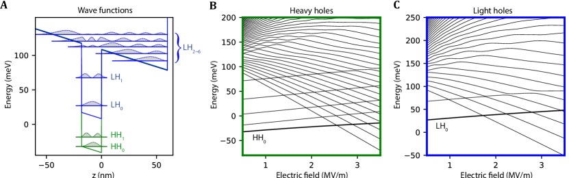
Figure 2: A, The potential of the heterostructure along the growth direction and the $\rm n^{th}$ sub-band of the heavy (light) hole levels $\rm HH_{n}$ ($\rm LH_{n}$). For this plot the electric field strength is $F_{z}=0.5\,\mathrm{MV/m}$. B, C, The energy levels of the $\rm n^{th}$ heavy hole sub-bands and the light hole sub-bands. The levels with negative slope are located in the quantum well, while levels with the a positive slope spread outside the quantum well.

The effect of strain in the Ge well in between the SiGe laysers is described by the Pikus-Bir Hamiltonian (see appendix). Assuming uniaxial strain ($\epsilon_{xy}=\epsilon_{xz}=\epsilon_{yz}=0$) the strain operators become a constant in the different materials. This allows us to describe the effect of strain and an applied electric field in the $z$-direction using the following potential

$$V_{\perp}(z)=-eF_{z}\,z-\begin{cases}0,&0<z<d_{i}\\ U_{l},&-d_{w}<z<0\\ 0,&z<-d_{w}\end{cases}.$$ (11)

Here, $d_{w}$ is the thickness of the strained-Ge quantum well, $d_{i}$ is the thickness of the $\rm Si_{0.2}Ge_{0.8}$ top layer, $F_{z}$ is the out-of-plane electric field necessary for hole accumulation, $e$ is the elementary charge, and $U_{l}$ is the band-offset of the heavy-hole ($l=\text{HH}$) and light hole ($l=\text{LH}$) for the strained Ge layer (see appendix). The SiGe/Ge/SiGe heterostructure is capped by a $\text{SiO}_{2}$ top interface which is considered to have infinite potential with appropriate boundary conditions $\Psi(z=a_{w})=0$. An illustration is shown in Fig. 2A. The in-plane confinement is modelled as a harmonic potential $V_{\parallel}(x,y)=\frac{1}{2}m_{p}\omega_{0}^{2}(x^{2}+y^{2})$. The magnetic field has a magnitude of $B=0.1\,\mathrm{T}$ for the simulations presented in this work if not mentioned explicitly. The magnetic field has an angle $\theta$ from the x-axis. The strength of the harmonic potential $m_{p}\omega^{2}_{0}=\frac{\gamma_{1}+\gamma_{2}}{m_{0}}(\frac{\hbar^{2}}{a^{4}_{0}}-\frac{e^{2}B^{2}_{z}}{4})$ with $a_{0}=50\,\mathrm{nm}$. This setting makes the in-plane heavy hole ground state wave function have a constant radius of 50 nm for different magnetic field angles.

The last term in Eq. (1) $H_{\text{Zeeman}}=2\mu_{B}\kappa\,\boldsymbol{J}\cdot\boldsymbol{B}+2\mu_{B}q(J_{x}^{3}B_{x}+J_{y}^{3}B_{y}+B_{z}^{3}B_{z})$ describes the interaction between the hole spin and the magnetic field, where $\mu_{B}=e\hbar/(2m_{0})$ is Bohr’s magneton, $\boldsymbol{B}=(B_{x},B_{z},B_{z})^{T}$ the magnetic field, $\boldsymbol{J}=(J_{x},J_{y},J_{z})^{T}$ the vector consisting of the Spin-$\frac{3}{2}$ matrices, and $\kappa=3.41\,\mathrm{}$ and $q=0.067\,\mathrm{}$ the isotropic and an-isotropic Zeeman coefficients for Ge [26].

I.2 Simulation of g-factor of the ground state

The total Hamiltonian Eq. (6) is projected on a set of basis states and then diagonalized numerically. The basis vectors in our simulations consist of product states $\Psi^{H(L)}_{H(L),j,k}(x,y,z)=\phi^{H(L)}_{j}(x,y)\psi^{H(L)}_{k}(z)$ which are given by independently solving the in-plane and out-of-plane effective mass Schroedinger equation for the heavy-hole and light-hole bands. The in-plane orbital wave functions are Fock-Darwin states labelled as $\ket{n,n_{z}}$. The z-direction sub-bands of heavy (light) holes $\rm HH_{n}$ ($\rm LH_{n}$) have the form of piece-wise Airy functions [27, 28] with Ben-Daniel–Duke boundary conditions (see appendix) $\psi_{p}(z=a)=\psi_{q}(z=a)$ and $\partial_{z}\psi_{p}(z=a)=\partial_{z}\psi_{q}(z=a)$ with $(p,q)=(\text{Si}_{0.2}\text{Ge}_{0.8},\text{Ge}),(\text{Ge},\text{Si}_{0.2}\text{Ge}_{0.8})$ and $a=0,-d_{w}$. Calculations involving higher orbital states in the realistic heterostructures are computationally expensive.

As the first attempt to simulate sweet spots in the realistic systems, we only considered the effective potentials created in the region of $\text{Si}_{0.2}\text{Ge}_{0.8}$ and Ge, while neglecting the difference of other material parameters such as the Luttinger parameters and Zeeman coefficients. Fig. 2. shows the lowest sub-band states in the heterostructure. The wave-functions of the sub-bands can be separated into states which are localized inside the quantum well, localized at the triangular potential at the surface, or delocalized between well and top-interface similar to the bonding and anti-bonding orbitals. For electric fields $F_{z}<3.5\,\mathrm{MV/m}$, there are five heavy hole states and two light hole states completely localized inside the quantum well as indicated by the spectrum in Fig. 2B and 2C. Note, that for larger electric fields first the light hole states and later the heavy states ”leak” out of the quantum well. The heavy hole ground state stays inside the quantum well for the electric field lower than $F_{z}\approx 2.5\,\mathrm{MV/m}$ which marks the upper limit of electric field in this work. We choose three heavy hole sub-band and 1 to 57 light hole sub-bands to simulate the Zeeman splittings of the heavy hole ground state, which we will justify as a sufficient set. The effective g-factor $g(F_{z})$ is then the ratio between Zeeman splitting and the magnetic field strength (set to $B=0.1\,\mathrm{T}$ in our simulations).

I.3 Simulation of the dephasing time

In order to estimate the performance of the planar hole qubits we further compute the effective dephasing times in the presence of charge noise. We model charge noise as random fluctuations of the electric field. For the electric field fluctuations we assume that the noise follows a $S(w)=A^{2}/f$ spectral density [29, 9]. To efficiently model the dynamics due to charge noise, we make two additional assumptions. First we only assume fluctuations of the electric field in z-directions and neglect in-plane fluctuations due to their vanishing impact. This is well justified in planar quantum dots due to the smooth potential landscape in $x,y$-plane from the electrostatic confinement. However, note that this assumption may break in the presence of atomistic interface steps or stray strain from metallic gates [30]. Second we assume that the noise is coupled to the qubit linearly [31]. The pure dephasing time is then given by

$$T_{2}^{\star}(F_{z})=\frac{\hbar}{A\sqrt{\log(r)}\left|\mu_{B}\frac{\partial g(F_{z})}{\partial F_{z}}B\right|}.$$ (12)

Here, $g(F_{z})$ is the effective g-factor of the ground state and bandwith $r=1.68\,\times 10^{9}$ is the ratio of the lower and higher frequency cutoff. Because of the finite numbers of basis states included in our simulations and the finite step size in electric field, the g-factor is not completely a smooth function giving rise to local variations that overshadow the general trend of $\frac{\partial g(F_{z})}{\partial F_{z}}$. Since these local variations are mostly an artifact of our simulations and our interest lies in the general trend the interpolated g-factor $g(F_{z})$ is fitted to a fourth order polynomial here. Sweets spots are defined by a vanishing linear noise coupling $\frac{\partial g(F_{z})}{\partial F_{z}}=0$. Note that a sweet spot does not give rise to infinite $T_{2}^{\star}$ but requires a more sophisticated treatment [32]. The electric field noise is estimated to be $A=3.5\,\mathrm{kV/m}$ inside the quantum well, based on the charge noise estimation [33] and the Poisson-Schrodinger simulation including metal/dielectrics gate layers and the germanium heterostructure [34].

Since the dephasing time as well as the qubit resonance frequency is strongly dependent on the magnitude of the applied magnetic field due to the strong g-factor anisotropy a comparison of $T_{2}^{\star}$ with fixed magnetic field is significantly favoring small g-factors. To provide a well motivated comparison we renormalize $T_{2}^{\star}$ to a fixed qubit frequency instead.

II Results

II.1 Out-of-plane g-factor and convergence behavior

The out-of-plane g-factor strongly depends on the electric field, as shown in Fig. 3A. The g-factor and its derivative changes significantly with the choice of the light hole states. If we only consider the states in the quantum well, the g-factor is monotonically increasing with respect to the electric field. By incorporating the highly excited light hole states (up to the $\rm 56^{th}$ excited state in this work), the g-factor changes and is monotonically decreasing with respect to electric field. The zero-derivative point, i.e. the sweet spot, is not observed in the range of electric field considered here. Applying larger electric fields would result in a ground state that is not located in the quantum well and therefore not considered. Our simulated g-factors match qualitatively with experiments using Hall-Bar measurements at low density [6, 35].

We investigate the dependence of the choice of the light hole levels in Fig. 3B. The g-factor converges slowly indicating the high energy light hole states are not negligible for the estimation of the g-factor. We remark that going beyond the current light hole states the 4-band model is insufficient to accurately describes the physics and the split-off-band (or even more bands) has to be included.

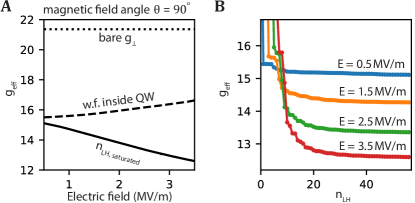
Figure 3: A, The out-of-plane g-factor as a function of electric field. The solid curve is the g-factor obtained by including $\rm n_{LH,saturated}=57$ light hole states in the simulation. The dashed curve is the g-factor obtained by simulating the light hole states located in the germanium quantum well. B, The g-factor as a function of light hole level numbers $\rm n_{LH}$. Curves in different colors are the results taken at different electric field.

II.2 In-plane g-factor

The in-plane g-factor is plotted in Fig. 4A. Compared to the out-of-plane g-factor, the in-plane g-factor is much smaller and it has weaker dependence on the electric field. The g-factor is monotonically increasing with respect to the electric field in both choice of light hole states, as shown in the dashed and solid curves in Fig. 4A. The g-factor dependence of the light hole levels is plotted in Fig. 3B. Our simulation results match the measured g-factors $g=0.2\pm 0.1\,\mathrm{}$ in devices using the same heterostructure [9], where the large spread can be attributed to non-circular confinement [8]. The slow convergence is qualitatively similar to the g-factor dependence for out-of-plane magnetic fields. In general operating planar hole qubits in in-plane magnetic field direction will result in longer coherence time than for out-of-plane magnetic fields.

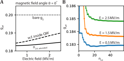
Figure 4: A, The in-plane g-factor as a function of electric field. The solid curve is the g-factor obtained by including $\rm n_{LH,saturated}=57$ light hole states in the simulation. The dashed curve is the g-factor obtained by simulating the light hole states located in the germanium quantum well. B, The g-factor as a function of light hole level numbers $\rm n_{LH}$. Curves in different colors are the results taken at different electric field.

II.3 Optimal magnetic field angle

The opposite dependence of the g-factor on electric field for in-plane and out-of-plane magnetic fields suggests that an optimal field angle exists where the g-factor is first-order insensitive to changes in the electric field. We expect the optimal magnetic field angle close to $\theta=\arctan(g_{\parallel}/g_{\perp})/3$ (see appendix). We therefore investigate the angle dependence, shown in Fig. 5A. The g-factor as a function of electric field becomes very flat for angles $\theta=\rm 0.15^{\circ}-0.20^{\circ}$. For certain magnetic field angles the Zeeman splitting becomes insensitive to electric field fluctuation over a wide range of electric fields values and thus enhancing spin coherence times. Fig. 5B shows the estimated dephasing time as a function of electric field at various magnetic field angles that form sweet spots. From the plot we find an optimal magnetic field angle of $\theta=\rm 0.2^{\circ}$ if we operate the hole spin qubit at electric field around $F_{z}=\rm 1\sim 1.5\,\mathrm{MV/m}$. The optimal field angle is decreased if we operate the qubit at lower electric field. We note that current vector magnets already satisfy the required precision. While we did not directly investigate the Rabi frequency directly at the sweet spot, off-diagonal g-factor components are maximized at this angle indicating fast qubit operations combined with long coherence times. Additionally, the ability to shift the sweet spot for different electric field allows to compensate local variation opening the possibility to a scalable architecture.

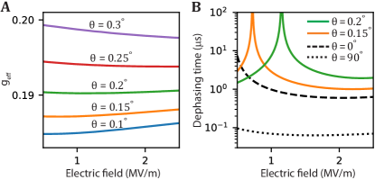
Figure 5: A, The g-factor as a function of electric field with different magnetic field angle when considering $\rm n_{LH}=57$ light hole levels. B, Dephasing time as a function of electric field at different magnetic field angle and strength. The magnetic field strength is chosen such that for each angle the Zeeman splittings are equal (2.5 GHz) at an electric field of $F_{z}=0.5\,\mathrm{MV/m}$.

III Conclusion

In conclusion, we simulated the effective g-factor of the hole spins in planar germanium heterostructures and studied its dependence on the electric field, the magnetic field orientation and the light hole level numbers. We observed that the excited light hole levels which are not confined by the quantum well have non-negligible contribution to the g-factor and its derivative with respect to the electric field. When including those light hole levels, we found a tunable sweet spot of the g-factor with respect to electric field if the magnetic field angle is close to in-plane direction. We note that recent experimental work reporting a sweet spot for holes in silicon FinFet supports the opportunity for sweet spots for holes in planar germanium [36]. Decoherence is currently a bottleneck for scaling planar germanium hole qubits [9] thus operating at (scalable) sweet spots may therefore enable the next step in advancing to larger quantum circuits.

We presented proof-of-principle simulation results by including higher levels and a realistic heterostructure potential. To make the simulation more realistic, we can incorporate the split-off bands and the spatial dependent material parameters of the heterostructures (e.g. Luttinger parameters and Zeeman coefficients) in the future. Our model can be extended to study the response of hole qubits to driving (EDSR), decoherence from time-dependent charge noise, and g-factor variability from imperfect interfaces and shear-strain.

Acknowledgements

We acknowledge helpful discussions with M. Friesen, N. Hendrickx, S. Philips, H. Tidjani, A. Tosato, L. Vandersypen, and all members of the Vanderypen, Veldhorst, and Scappucci group. C.W. M. V. acknowledge support through an ERC Starting Grant. Research was sponsored by the Army Research Office (ARO) and was accomplished under Grant No. W911NF- 17-1-0274. The views and conclusions contained in this document are those of the authors and should not be interpreted as representing the official policies, either expressed or implied, of the Army Research Office (ARO), or the U.S. Government. The U.S. Government is authorized to reproduce and distribute reprints for Government purposes notwithstanding any copyright notation herein. M.R. acknowledges support from the Netherlands Organization of Scientific Research (NWO) under Veni grant VI.Veni.212.223.

Competing interests

The authors declare no competing interests.

Data availability

Simulation software and data analysis scripts supporting this work are available at 10.5281/zenodo.6949626.

Appendix A Derivation of the vertical confinement potential from strain tensor, band offset, and electric field

The vertical confinement $V_{\perp}(z)$ of the quantum dot consists of two contributions; alignment of the Fermi-energy of the heterostructure giving rise to a band offset and strain in the quantum well. The band offset is a constant for the different materials and can be experimentally measured or theoretically computed [37]. Strain is in general a $3\times 3$ strain tensor $\epsilon$ for each band and its effect on the hole states is described by the Pikus-Birr Hamiltonian. For simplifications we only consider in this paper the effect of hydrostatic strain and uniaxial strain and ignore all shear-strain components ($\epsilon_{xy}=\epsilon_{xz}=\epsilon_{yz}=0$). Consequently, the Pikus-Bir Hamiltonian becomes diagonal in the heavy-hole and light-hole basis $\ket{j,m_{j}}=\{\ket{\frac{3}{2},\frac{3}{2}},\ket{\frac{3}{2},-\frac{3}{2}},\ket{\frac{3}{2},\frac{1}{2}},\ket{\frac{3}{2},-\frac{1}{2}}\}$

$$H_{\text{PB}}=\text{diag}(P_{\epsilon}+Q_{\epsilon},P_{\epsilon}+Q_{\epsilon},P_{\epsilon}-Q_{\epsilon},P_{\epsilon}-Q_{\epsilon})$$ (13)

with the coefficients

$$P_{\epsilon}=-a_{V}(\epsilon_{xx}+\epsilon_{yy}+\epsilon_{zz}),$$ (14)

$$Q_{\epsilon}=-\frac{b_{V}}{2}(\epsilon_{xx}+\epsilon_{yy}-2\epsilon_{zz}),$$ (15)

where $a_{V}$ and $b_{V}$ are the deformation potentials which strongly depend on the silicon concentration $x$ in the $\text{Si}_{x}\text{Ge}_{1-x}$ layer of the heterostructure. For $x=20\%$ we use $a_{V}=2.0\,\mathrm{eV}$ and $b_{V}=-2.16\,\mathrm{eV}$ [3].

Since strain is only present in the quantum well and only depends on the band $j=\frac{1}{2},\frac{3}{2}$ and not the sign of the spin we can rewrite the effect of the band offset and strain as an effective potential of the form

$$V_{\perp}(z)=-\begin{cases}0,&0<z<d_{i}\\ U_{l},&-d_{w}<z<0\\ 0,&z<-d_{w}\end{cases},$$ (16)

where $l=\text{HH},\text{LH}$ denotes the band. Note, that solely due to the uniaxial strain components the heavy and light-hole degeneracy is lifted inside the quantum well. For our simulations we use the following parameters $U_{\text{HH}}=150\,\mathrm{meV}$ and $U_{\text{LH}}=100\,\mathrm{meV}$ extracted from [37] and coincides with the values from [3]. Adding a global electric potential $-eF_{z}z$ originating from the metallic plunger gate on top we end up with expression (11) in the main text.

Appendix B Derivation of the analytical wavefunctions and numerical simulation

The total Hamiltonian Eq. (1) is projected on a set of basis states and then diagonalized numerically. The basis states for the heavy-hole (light-hole) are product states of in-plane Fock-Darwin wave functions $\phi^{H(L)}_{j}(H(L),x,y)$ and the derived wave-functions in z-direction consisting of piece-wise Airy functions

$$\Psi^{H(L)}_{{H(L)},j,k}(x,y,z)=\phi^{H(L)}_{j}(x,y)\psi^{H(L)}_{k}(z),$$ (17)

with

$$\psi^{H(L)}_{k}(z)=\begin{cases}c^{H(L)}_{k,1}Ai\left(u_{H(L)}-\epsilon^{H(L)}_{k}-z/\zeta_{0}^{H(L)}\right)+c^{H(L)}_{k,2}Bi\left(u_{H(L)}-\epsilon^{H(L)}_{k}-z/\zeta_{0}^{H(L)}\right),&0<z<d_{i}\\ c^{H(L)}_{k,3}Ai\left(-\epsilon^{H(L)}_{k}-z/\zeta_{0}^{H(L)}\right)+c^{H(L)}_{k,4}Bi\left(-\epsilon^{H(L)}_{k}-z/\zeta_{0}^{H(L)}\right),&-d_{w}<z<0\\ c^{H(L)}_{k,5}Ai\left(u_{H(L)}-\epsilon^{H(L)}_{k}-z/\zeta_{0}^{H(L)}\right),&z<-d_{w}\end{cases}.$$ (18)

Here, $Ai$ and $Bi$ are the conventional Airy functions, $\zeta_{0}^{H(L)}=(\hbar^{2}/(2m_{L(H)}eF_{z}))^{\frac{1}{3}}$ and $E_{\text{tri}}^{H(L)}=\hbar^{2}/(2m_{H(L)}\zeta_{0}^{H(L)})$ are the effective confinement length and energy of the triangular potential, ${u_{H(L)}=U_{H(L)}/E_{\text{tri}}^{H(L)}}$ is the effective potential barrier, and $\epsilon^{H(L)}_{k}=E^{H(L)}_{k}/E_{\text{tri}}^{H(L)}$ is the effective eigenenergy of the heavy hole (light hole) sub-band $k$. The weighting factors $c^{H(L)}_{k,n}$ are defined via the Ben-Daniel–Duke boundary conditions [27, 28] $\psi_{p}(z=a)=\psi_{q}(z=a)$ and $\frac{1}{m^{\star}_{p}}\partial_{z}\psi_{p}(z=a)=\frac{1}{m^{\star}_{q}}\partial_{z}\psi_{q}(z=a)$ with $(p,q)=(\text{Si}_{0.2}\text{Ge}_{0.8},\text{Ge}),(\text{Ge},\text{Si}_{0.2}\text{Ge}_{0.8})$ and $a=0,-d_{w}$. Assuming that the effective masses of the heavy hole (light hole) in SiGe is identical to the Ge effective masses, i.e. $m_{\perp,\text{Ge}}^{H(L)}=m_{\perp,\text{SiGe}}^{H(L)}$ and $m_{\parallel,\text{Ge}}^{H(L)}=m_{\parallel,\text{SiGe}}^{H(L)}$, the boundary conditions become independent of the effective mass and we arrive at the expressions in the main text. We find the eigenenergies $E^{H(L)}_{k}$ of the heavy hole (light hole) band via the boundary conditions in Eq. (11) following Ref. [28] but translate it to a computational task of finding roots of a fifth-order polynomial of the Airy functions. The roots are solved numerically using the Reduce-function in Mathematica. Afterwards we check and add missing roots using a bisection algorithm.

The in-plane orbital wave-fucntions are solution of a 2D harmonic confinement in the presence of a magnetic field. The general solutions are the Fock-Darwin states

$$\phi^{H(L)}_{j=(n,l)}(x,y)= \left(\frac{x^{2}+y^{2}}{a_{B,H(L)}}\right)^{\frac{|l|}{2}}\mathcal{L}_{n}^{|l|}\left(\frac{x^{2}+y^{2}}{a_{B,H(L)}}\right)$$

$$\times\exp(i\,l\arctan(y/x)),$$ (19)

where $\mathcal{L}_{n}^{|l|}(\xi)$ is the generalized Laguerre polynomial, $a_{B,H(L)}=$ and $j$ is ordered in terms of ascending eigenenergy.

For both heavy hole and light hole, we use a fixed number of 15 in-plane orbital wave functions. The expression and the integrals between the in-plane orbits are computed analytically. In z-direction, we consider three heavy hole sub-bands and $n_{LH}$ light hole sub-bands. We observe that the g-factors changes with $n_{LH}$ and saturates as $n_{LH}$ increases. The largest $n_{LH}$ we consider is 57. Contrarily, the number of heavy hole sub-bands has a significant smaller impact on the g-factor. The numbers of basis states are $45$ and $15n_{LH}$ for heavy hole and light hole. The total dimension of the Hamiltonian is $90+30\times n_{LH}$.

To find the electric field dependence of the g-factor, the above procedure is repeated for values of electric field in the interval $F_{z}=0.5-3.5\,\mathrm{MV/m}$, with the step size of $\Delta F_{z}=5\times 10^{-3}\,\mathrm{MV/m}$. For each electric field value we compute the z-direction sub-bands of the heavy hole and light hole, construct the basis states, compute the projected total Hamiltonian Eq. (1), diagonalize the matrix, and finally obtain the effective g-factor, the ratio of Zeeman splitting to the magnetic field strength, of the heavy hole ground state.

Appendix C Optimal magnetic field angle

The emergence of an optimal magnetic field angle can be derived from Hamiltonian (1) of the main text. While this derivation can be easily generalized to arbitrary magnetic fields we pursue a magnetic field in the $xz$-plane $\boldsymbol{B}=(B\cos(\theta),0,B\sin(\theta))^{T}$. To diagonalize the heavy-hole state sector we apply the unitary rotation $U=e^{-i\phi\sigma_{y}/2}$ with $\sigma_{z}$ being the Pauli matrix acting only on the heavy-hole space and

$$\phi=\arctan\left(\frac{4\kappa+9q}{2q}\tan(\theta)\right)=\arctan\left(\frac{g_{\perp}}{g_{\parallel}}\tan(\theta)\right).$$ (20)

Here, $\kappa$ and $q$ are the isotropic and an-isotropic Zeeman coefficients and $g_{\perp}=6\kappa+27q/2$ and $g_{\parallel}=3q$ are the out-of-plane and in-plane pure heavy hole g-factors. While the angle $\theta$ describes the rotation of the magnetic field, the angle $\phi$ describes the rotation of the heavy-hole quantization axis. Minimal variation of the g-factor is then expected to be close to $\phi=45\,\mathrm{{}^{\circ}}$ where the orbital contributions from in-plane and out-of-plane magnetic fields compensate each other due to the different slopes. From our simulations we can see that the ratio of the slopes $\frac{\partial g(F_{z})}{\partial F_{z}}$ normalized to equal qubit frequencies for $\theta=90\,\mathrm{{}^{\circ}}$ and $\theta=0\,\mathrm{{}^{\circ}}$ we end up with $\theta_{\text{opt}}\approx\arctan(g_{\parallel}/g_{\perp})/3$.

References

- Vandersypen et al. [2017] L. M. K. Vandersypen, H. Bluhm, J. S. Clarke, A. S. Dzurak, R. Ishihara, A. Morello, D. J. Reilly, L. R. Schreiber, and M. Veldhorst, Interfacing spin qubits in quantum dots and donors—hot, dense, and coherent, npj Quantum Information 3, 1 (2017).
- Scappucci et al. [2020] G. Scappucci, C. Kloeffel, F. A. Zwanenburg, D. Loss, M. Myronov, J.-J. Zhang, S. De Franceschi, G. Katsaros, and M. Veldhorst, The germanium quantum information route, Nature Reviews Materials , 1 (2020).
- Terrazos et al. [2021] L. A. Terrazos, E. Marcellina, Z. Wang, S. N. Coppersmith, M. Friesen, A. R. Hamilton, X. Hu, B. Koiller, A. L. Saraiva, D. Culcer, and R. B. Capaz, Theory of hole-spin qubits in strained germanium quantum dots, Physical Review B 103, 125201 (2021).
- Hendrickx et al. [2018] N. W. Hendrickx, D. P. Franke, A. Sammak, M. Kouwenhoven, D. Sabbagh, L. Yeoh, R. Li, M. L. V. Tagliaferri, M. Virgilio, G. Capellini, G. Scappucci, and M. Veldhorst, Gate-controlled quantum dots and superconductivity in planar germanium, Nature Communications 9, 2835 (2018).
- Watzinger et al. [2018] H. Watzinger, J. Kukučka, L. Vukušić, F. Gao, T. Wang, F. Schäffler, J.-J. Zhang, and G. Katsaros, A germanium hole spin qubit, Nature Communications 9, 3902 (2018).
- Lodari et al. [2019] M. Lodari, A. Tosato, D. Sabbagh, M. A. Schubert, G. Capellini, A. Sammak, M. Veldhorst, and G. Scappucci, Light effective hole mass in undoped Ge/SiGe quantum wells, Physical Review B 100, 041304 (2019).
- Hendrickx et al. [2020] N. W. Hendrickx, D. P. Franke, A. Sammak, G. Scappucci, and M. Veldhorst, Fast two-qubit logic with holes in germanium, Nature 577, 487 (2020).
- Jirovec et al. [2022] D. Jirovec, P. M. Mutter, A. Hofmann, A. Crippa, M. Rychetsky, D. L. Craig, J. Kukucka, F. Martins, A. Ballabio, N. Ares, D. Chrastina, G. Isella, G. Burkard, and G. Katsaros, Dynamics of Hole Singlet-Triplet Qubits with Large -Factor Differences, Physical Review Letters 128, 126803 (2022).
- Hendrickx et al. [2021] N. W. Hendrickx, W. I. L. Lawrie, M. Russ, F. van Riggelen, S. L. de Snoo, R. N. Schouten, A. Sammak, G. Scappucci, and M. Veldhorst, A four-qubit germanium quantum processor, Nature 591, 580 (2021).
- Lawrie et al. [2021] W. I. L. Lawrie, M. Russ, F. van Riggelen, N. W. Hendrickx, S. L. de Snoo, A. Sammak, G. Scappucci, and M. Veldhorst, Simultaneous driving of semiconductor spin qubits at the fault-tolerant threshold, arXiv:2109.07837 (2021).
- van Riggelen et al. [2022] F. van Riggelen, W. I. L. Lawrie, M. Russ, N. W. Hendrickx, A. Sammak, M. Rispler, B. M. Terhal, G. Scappucci, and M. Veldhorst, Phase flip code with semiconductor spin qubits, arXiv:2202.11530 (2022).
- Stano and Loss [2021] P. Stano and D. Loss, Review of performance metrics of spin qubits in gated semiconducting nanostructures, arXiv:2107.06485 (2021).
- Froning et al. [2021] F. N. M. Froning, M. J. Rančić, B. Hetényi, S. Bosco, M. K. Rehmann, A. Li, E. P. A. M. Bakkers, F. A. Zwanenburg, D. Loss, D. M. Zumbühl, and F. R. Braakman, Strong spin-orbit interaction and -factor renormalization of hole spins in Ge/Si nanowire quantum dots, Physical Review Research 3, 013081 (2021).
- Wang et al. [2022] K. Wang, G. Xu, F. Gao, H. Liu, R.-L. Ma, X. Zhang, Z. Wang, G. Cao, T. Wang, J.-J. Zhang, D. Culcer, X. Hu, H.-W. Jiang, H.-O. Li, G.-C. Guo, and G.-P. Guo, Ultrafast coherent control of a hole spin qubit in a germanium quantum dot, Nature Communications 13, 206 (2022).
- Stano et al. [2018] P. Stano, C.-H. Hsu, M. Serina, L. C. Camenzind, D. M. Zumbühl, and D. Loss, -factor of electrons in gate-defined quantum dots in a strong in-plane magnetic field, Physical Review B 98, 195314 (2018).
- Bosco et al. [2021a] S. Bosco, B. Hetényi, and D. Loss, Hole Spin Qubits in Si FinFETs with fully tunable spin-orbit coupling and Sweet Spots for Charge Noise, PRX Quantum 2, 010348 (2021a).
- Bosco and Loss [2022] S. Bosco and D. Loss, Hole spin qubits in thin curved quantum wells, arXiv:2204.08212 (2022).
- Wang et al. [2021] Z. Wang, E. Marcellina, A. R. Hamilton, J. H. Cullen, S. Rogge, J. Salfi, and D. Culcer, Optimal operation points for ultrafast, highly coherent Ge hole spin-orbit qubits, npj Quantum Information 7, 1 (2021).
- Adelsberger et al. [2022] C. Adelsberger, M. Benito, S. Bosco, J. Klinovaja, and D. Loss, Hole-spin qubits in ge nanowire quantum dots: Interplay of orbital magnetic field, strain, and growth direction, Phys. Rev. B 105, 075308 (2022).
- Bosco et al. [2021b] S. Bosco, M. Benito, C. Adelsberger, and D. Loss, Squeezed hole spin qubits in Ge quantum dots with ultrafast gates at low power, Physical Review B 104, 115425 (2021b).
- Lodari et al. [2021] M. Lodari, N. W. Hendrickx, W. I. L. Lawrie, T.-K. Hsiao, L. M. K. Vandersypen, A. Sammak, M. Veldhorst, and G. Scappucci, Low percolation density and charge noise with holes in germanium, Materials for Quantum Technology 1, 011002 (2021).
- Wimbauer et al. [1994] T. Wimbauer, K. Oettinger, A. L. Efros, B. K. Meyer, and H. Brugger, Zeeman splitting of the excitonic recombination in As/GaAs single quantum wells, Physical Review B 50, 8889 (1994).
- Del Vecchio et al. [2020] P. Del Vecchio, M. Lodari, A. Sammak, G. Scappucci, and O. Moutanabbir, Vanishing Zeeman energy in a two-dimensional hole gas, Physical Review B 102, 115304 (2020).
- Semina et al. [2021] M. A. Semina, A. A. Golovatenko, and A. V. Rodina, Influence of the spin-orbit split-off valence band on the hole factor in semiconductor nanocrystals, Physical Review B 104, 205423 (2021).
- Stano et al. [2019] P. Stano, C.-H. Hsu, L. C. Camenzind, L. Yu, D. Zumbühl, and D. Loss, Orbital effects of a strong in-plane magnetic field on a gate-defined quantum dot, Physical Review B 99, 085308 (2019).
- Winkler [2003] R. Winkler, Spin-Orbit Coupling Effects in Two-Dimensional Electron and Hole Systems (Springer Tracts in Modern Physics) (2003).
- Harrison and Valavanis [2016] P. Harrison and A. Valavanis, Quantum Wells, Wires and Dots: Theoretical and Computational Physics of Semiconductor Nanostructures, fourth edition ed. (Chichester, West Sussex, United Kingdom ; Hoboken, NJ, USA, 2016).
- Hosseinkhani and Burkard [2020] A. Hosseinkhani and G. Burkard, Electromagnetic control of valley splitting in ideal and disordered Si quantum dots, Physical Review Research 2, 043180 (2020).
- Paladino et al. [2014] E. Paladino, Y. M. Galperin, G. Falci, and B. L. Altshuler, 1/f noise: Implications for solid-state quantum information, Rev. Mod. Phys. 86, 361 (2014).
- Pateras et al. [2018] A. Pateras, J. Park, Y. Ahn, J. A. Tilka, M. V. Holt, C. Reichl, W. Wegscheider, T. A. Baart, J. P. Dehollain, U. Mukhopadhyay, L. M. K. Vandersypen, and P. G. Evans, Mesoscopic Elastic Distortions in GaAs Quantum Dot Heterostructures, Nano Letters 18, 2780 (2018).
- Ithier et al. [2005] G. Ithier, E. Collin, P. Joyez, P. J. Meeson, D. Vion, D. Esteve, F. Chiarello, A. Shnirman, Y. Makhlin, J. Schriefl, and G. Schaan, Decoherence in a superconducting quantum bit circuit, Phys. Rev. B 72, 134519 (2005).
- Makhlin and Shnirman [2004] Y. Makhlin and A. Shnirman, Dephasing of Solid-State Qubits at Optimal Points, Phys. Rev. Lett. 92, 178301 (2004).
- Xue et al. [2022] X. Xue, M. Russ, N. Samkharadze, B. Undseth, A. Sammak, G. Scappucci, and L. M. K. Vandersypen, Quantum logic with spin qubits crossing the surface code threshold, Nature 601, 343 (2022).
- Tosato et al. [2022] A. Tosato, B. Ferrari, A. Sammak, A. R. Hamilton, M. Veldhorst, M. Virgilio, and G. Scappucci, A High-Mobility Hole Bilayer in a Germanium Double Quantum Well, Advanced Quantum Technologies 5, 2100167 (2022).
- Lodari et al. [2022] M. Lodari, O. Kong, M. Rendell, A. Tosato, A. Sammak, M. Veldhorst, A. R. Hamilton, and G. Scappucci, Lightly strained germanium quantum wells with hole mobility exceeding one million, Applied Physics Letters 120, 122104 (2022).
- Piot et al. [2022] N. Piot, B. Brun, V. Schmitt, S. Zihlmann, V. P. Michal, A. Apra, J. C. Abadillo-Uriel, X. Jehl, B. Bertrand, H. Niebojewski, L. Hutin, M. Vinet, M. Urdampilleta, T. Meunier, Y.-M. Niquet, R. Maurand, and S. De Franceschi, A single hole spin with enhanced coherence in natural silicon, arXiv:2201.08637 (2022).
- Schäffler [1997] F. Schäffler, High-mobility Si and Ge structures, Semiconductor Science and Technology 12, 1515 (1997).