Unifying High- and Low-resolution Observations to Constrain the Dayside Atmosphere of KELT-20b/MASCARA-2b

Abstract

We present high-resolution dayside thermal emission observations of the exoplanet KELT-20b/MASCARA-2b using the MAROON-X spectrograph. Applying the cross-correlation method with both empirical and theoretical masks and a retrieval analysis, we confirm previous detections of Fe i emission lines and we detect Ni i for the first time in the planet (at 4.7$\sigma$ confidence). We do not see evidence for additional species in the MAROON-X data, including notably predicted thermal inversion agents TiO and VO, their atomic constituents Ti i and V i, and previously claimed species Fe ii and Cr i. We also perform a joint retrieval with existing Hubble Space Telescope/WFC3 spectroscopy and Spitzer/IRAC photometry. This allows us to place bounded constraints on the abundances of Fe i, H₂O, and CO, and to place a stringent upper limit on the TiO abundance. The results are consistent with KELT-20b having a solar to slightly super-solar composition atmosphere in terms of the bulk metal enrichment, and the carbon-to-oxygen and iron-to-oxygen ratios. However, the TiO volume mixing ratio upper limit (10^-7.6 at 99% confidence) is inconsistent with this picture, which, along with the non-detection of Ti i, points to sequestration of Ti species, possibly due to nightside condensation. The lack of TiO but the presence of a large H₂O emission feature in the WFC3 data is challenging to reconcile within the context of 1D self-consistent, radiative-convective models.

1 Introduction

Table 1: Log of the MAROON-X observations

UT Date	Exposures	Planet Phase Range	Airmass	Conditions	Seeing	Average Blue Arm SNR
2021 May 29 10:47 $\rightarrow$ 14:03	34	0.63 $\rightarrow$ 0.67	1.28 $\rightarrow$ 1.03	stable, clear	0.6″	176
2021 June 04 11:37 $\rightarrow$ 14:34	31	0.37 $\rightarrow$ 0.40	1.09 $\rightarrow$ 1.02 $\rightarrow$ 1.08	stable, clear	0.5″	196

KELT-20b/MASCARA-2b (hereafter KELT-20b for brevity) is a 1.56 $R_{\text{Jup}}$ radius exoplanet orbiting a bright ($m_{V}\sim 7.6$) A star with a 3.47 day orbital period (Lund et al., 2017; Talens et al., 2018). These parameters place it in the population of the $\sim 30$ known transiting hot Jupiters orbiting early-type stars. KELT-20b is very highly for dayside emission atmospheric follow-up due to the apparent magnitude of the host star, the size of the planet relative to the host star, and the planet’s high equilibrium temperature of $\sim$2250 K. Furthermore, the unambiguous detection of both iron (Borsa et al., 2022; Yan et al., 2022a; Johnson et al., 2022) and water (Fu et al., 2022) in the emission spectrum of this exoplanet, which is one of the coolest exoplanets with a detected thermal inversion, gives a special opportunity to unify ground-based, high-resolution and space-based, low-resolution observations of exoplanet atmospheres.

The thermal emission spectrum of KELT-20b has been previously observed with ground-based, high-resolution spectrographs by Borsa et al. (2022), Yan et al. (2022a), and Johnson et al. (2022). Using data from HARPS-N, Borsa et al. (2022) found a 6.8$\sigma$ detection of Fe i, as well as 3$\sigma$ detections of Fe ii and Cr i. The Borsa et al. (2022) detections of Fe ii and Cr i were only obtained for their post-secondary eclipse dataset and did not appear in their pre-eclipse dataset, thus suggesting the presence of chemical inhomogeneities. Yan et al. (2022a) used data from CARMENES and found Fe i at 7.5$\sigma$. Using PEPSI, Johnson et al. (2022) found Fe i in emission at 15.1$\sigma$ with non-detections of Fe ii and Cr i, among others. All the detected species in the previous works were observed in emission, which indicates a thermal inversion in KELT-20b’s atmosphere. Johnson et al. (2022) inferred upper limits on the abundances of their TiO, VO, FeH, and CaH non-detections with volume mixing ratios in the $\sim 10^{-9}-10^{-10}$ range, with the exception of FeH, for which they found at an upper limit of $3\times 10^{-7}$.

With space-based data, Fu et al. (2022) found H₂O and CO by analyzing the emission spectrum of KELT-20b derived from Hubble Space Telescope/WFC3 and Spitzer/IRAC eclipse observations. The water feature is the strongest of those in emission observed to-date with WFC3 (Mansfield et al., 2021). Fu et al. (2022) claimed that TiO is necessary to cause the deep inversion that leads to the large water emission feature. However, this requirement is in tension with the previous ground-based measurements that all failed to see TiO in KELT-20b’s thermal emission spectrum.

In this paper we present ground-based, high-resolution observations of the dayside emission from KELT-20b that were obtained using the MAROON-X instrument on the Gemini North telescope (Seifahrt et al., 2016, 2018, 2020). We aim to determine the composition of the planet’s dayside and perform a joint analysis including existing HST and Spitzer data to unify ground- and space-based results for this planet. We present our observations in §2. We describe two analyses of the data in §3 and 4 that yield the detection of the planet’s atmosphere and constraints on its properties. We contextualize our atmospheric retrieval with a comparison to atmospheric forward models in §5. We conclude with a discussion of the results in §6.

2 Observations

We used MAROON-X to obtain 4.51 hours of data (6.2 hours total observing time including overheads) of KELT-20b during a post-secondary eclipse phase on May 29 2021 and a pre-secondary eclipse phase on June 04 2021 UTC (Program ID: GN-2021A-Q119). We obtained data with both the MAROON-X “blue” (500 – 663 nm) and “red” (654 – 920 nm) channels. The two channels were observed simultaneously with 250 s exposures. Table 1 gives a log of the observations.

The data were reduced with the standard MAROON-X pipeline (Seifahrt et al., 2020). The pipeline includes detector calibration, one-dimensional spectral extraction, barycentric corrections calculated for the flux-weighted midpoint of each observation, and wavelength solutions and instrumental drift corrections based on the simultaneous Fabry-Perot etalon calibration data.

3 Detection of the Planetary Atmosphere Signal

We performed two analyses of our data to characterize KELT-20b’s dayside atmosphere. The first analysis used a cross-correlation function (CCF) technique with line-weighted binary templates following Pino et al. (2020) and Kasper et al. (2021). We used our established approach to create a time (i.e., phase) evolving spectrum containing planet lines normalized to the planet plus star continuum. We used eleven stellar templates built from observed stellar spectra (e.g., Suárez Mascareño et al., 2020) as masks for the CCF analysis. These masks correspond to F9, G2, G8, G9, K2, K6, M0, M2, M3, M4, and M5 stellar types and come from the ESPRESSO data reduction pipeline (“ESPRESSO DRS”). The mask ensemble spans the transition from ionized and neutral atoms to molecules as absorption features in stellar spectra. We used the masks in emission as analogs for the dayside of the hydrogen-dominated atmosphere of KELT-20b.

Figure 1 shows the peak signal-to-noise ratio (SNR) from the CCF analysis when combining the pre- and post-eclipse datasets and utilizing each of the masks. The SNR normalization was computed via a 3$\sigma$ background clipping method (as in Kasper et al., 2021). The high significance correlation with the earlier spectral type masks implicates neutral atomic lines, and Fe i in particular, as the dominant opacity source in KELT-20b’s atmosphere at the wavelengths probed. In comparison with the earlier-type masks applied to the blue channel, M-type masks give lower detection confidences, down to a non-detection at M5. Additionally, M-type masks do not yield a significant detection in the red channel. This indicates, in agreement with previous ground-based results, that molecules like TiO are likely not present in the planet’s atmosphere.

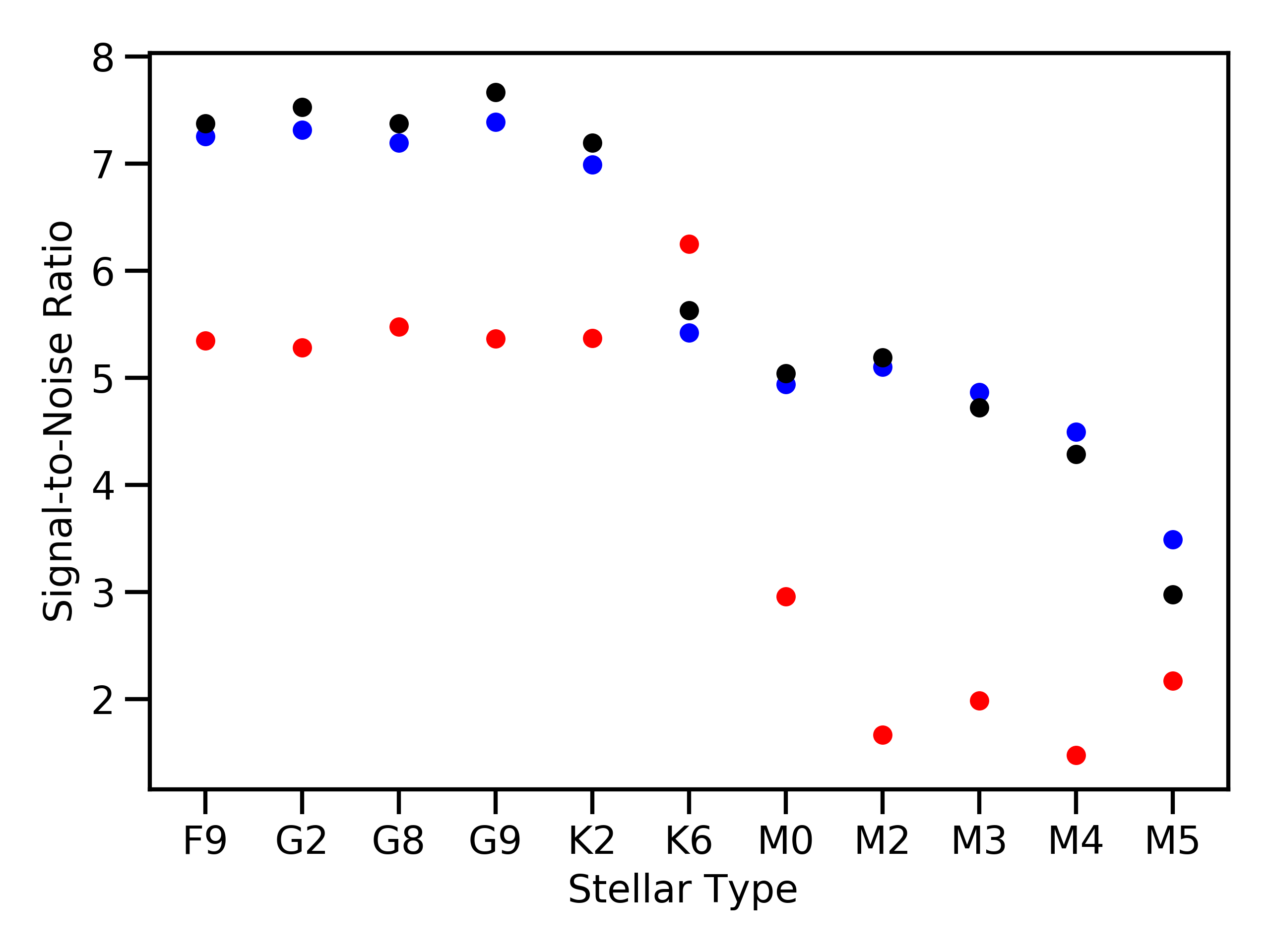
Figure 1: Detection SNR of the planetary atmospheric signal as a function of template stellar type. The responses of the red and blue channels are tracked individually by corresponding color. The combination of the two channels is shown in black.

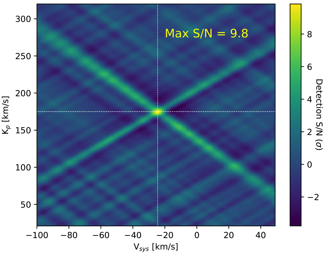
Figure 2: Map of the CCF in the planet velocity ($K_{p}$) vs. system velocity ($V_{\text{sys}}$) plane using the theoretical Fe i mask. Dotted lines correspond to the known system velocity and exoplanet orbital speed of -24.5 km s^-1 and 175 km s^-1, respectively, as in Borsa et al. (2022).

Complementary to the above analysis, we also explored the initial detectability of a variety of specific gases via data-model template cross-correlation (Kasper et al., 2021; Line et al., 2021). As in past works we removed stationary telluric and stellar features via the singular value decomposition method (we removed between 2-8 singular values and found little difference. We ultimately settled on 2 to prevent accidental removal of the planetary signal). The high-resolution template models are derived from the converged output of a KELT-20b-specific 1D radiative-convective-thermochemical equilibrium (1D-RC) model calculated using the ScCHIMERA code (Piskorz et al., 2018; Arcangeli et al., 2018; Mansfield et al., 2021; Kasper et al., 2021) assuming solar composition. The high-resolution model spectra are then convolved with a planetary rotation kernel and a Gaussian spectral response function at an R = 85,000, as appropriate for MAROON-X. We searched for CaH, Ca i and ii, CrH, Cr i, FeH, Fe i and ii, MgH, Mg i, Na i, Ni i, Si i, Ti i and ii, TiO, V i and ii, and VO.

Of all the species tested only Fe i and Ni i were found with a significant response (9.8$\sigma$ and 4.7$\sigma$, respectively). We also explored a grid of constant-with-altitude abundances for each gas (using the same converged temperature-pressure profile found above; e.g., Giacobbe et al., 2021) to ensure we did not miss any species detections due to the assumption of thermochemical equilibrium. No additional species were found in this analysis.

Figure 2 shows an SNR map for Fe i in the planet velocity (K_p) vs. system velocity (V${}_{\text{sys}}$) plane (a similar plot for Ni i can be found in the Appendix). The SNR in the map was computed via a 3-sigma background clipping method (as in Kasper et al., 2021). With the combination of pre- and post-eclipse phases we find agreement with the system velocity and planetary orbital speed. This $K_{p}$ vs. $V_{\text{sys}}$ mapping was also performed on the stellar template CCFs to ensure that the signal originated from the planet.

Table 2: Description of retrieved parameters and their prior ranges. All priors are assumed uniform between the bounds given. Variables correspond to the labeling in the corner plot shown in the Appendix.

Parameter	Description	Prior
$K_{p\text{,pre/post}}$	Keplerian velocity for	150 – 210 km s-1
	pre/post eclipse nights
$V_{\text{sys,pre/post}}$	systemic velocity	-50 – 10 km s-1
log($a_{\text{pre/post}}$)	model multiplicative	-1 – 1
	scale factor
log($\gamma_{1}$)	vis-to-IR opacity	-3 – 4
log($\kappa_{\text{IR}}$)	IR opacity	-3 – 0 (cgs)
T${}_{\text{irr}}$	irradiation temperature	1000 – 5000 K
$\Delta$log $g$	differential log-gravity	-1 – 0 (cgs)
	from max (log $g$=3.28)
H-, Fe, TiO,	log gas volume	-12 – 0
H2O, CO	mixing ratios
H*e-	log mixing ratio	-18 – 0
	hydrogen $\times$ electron
	for free-free cont.

4 Retrieval Analysis

Following Line et al. (2021) and Kasper et al. (2021), we applied the Brogi & Line (2019) cross-correlation-to-log-likelihood retrieval framework to derive abundances and the vertical temperature structure in KELT-20b’s dayside atmosphere. The CHIMERA forward model underlying the retrieval assumed constant-with-altitude abundances and used the Guillot (2010) parameterization of the temperature-pressure (T-P) profile. The retrieval parameters and their prior ranges are given in Table 2. A more detailed description of the radiative transfer method, including opacity sources, and log-likelihood implementation is given in Line et al. (2021) and Kasper et al. (2021) (with opacity sources there-in including McKemmish et al. (2019); John (1988); Grimm & Heng (2015); Grimm et al. (2021)) as well as new cross-sections utilized in this work from the EXOPLINES data base (Gharib-Nezhad et al., 2021) as sourced from the line lists for VO (McKemmish et al., 2016), H₂O (Polyansky et al., 2018), MgH (GharibNezhad et al., 2013), CrH and CaH (Bernath, 2020).

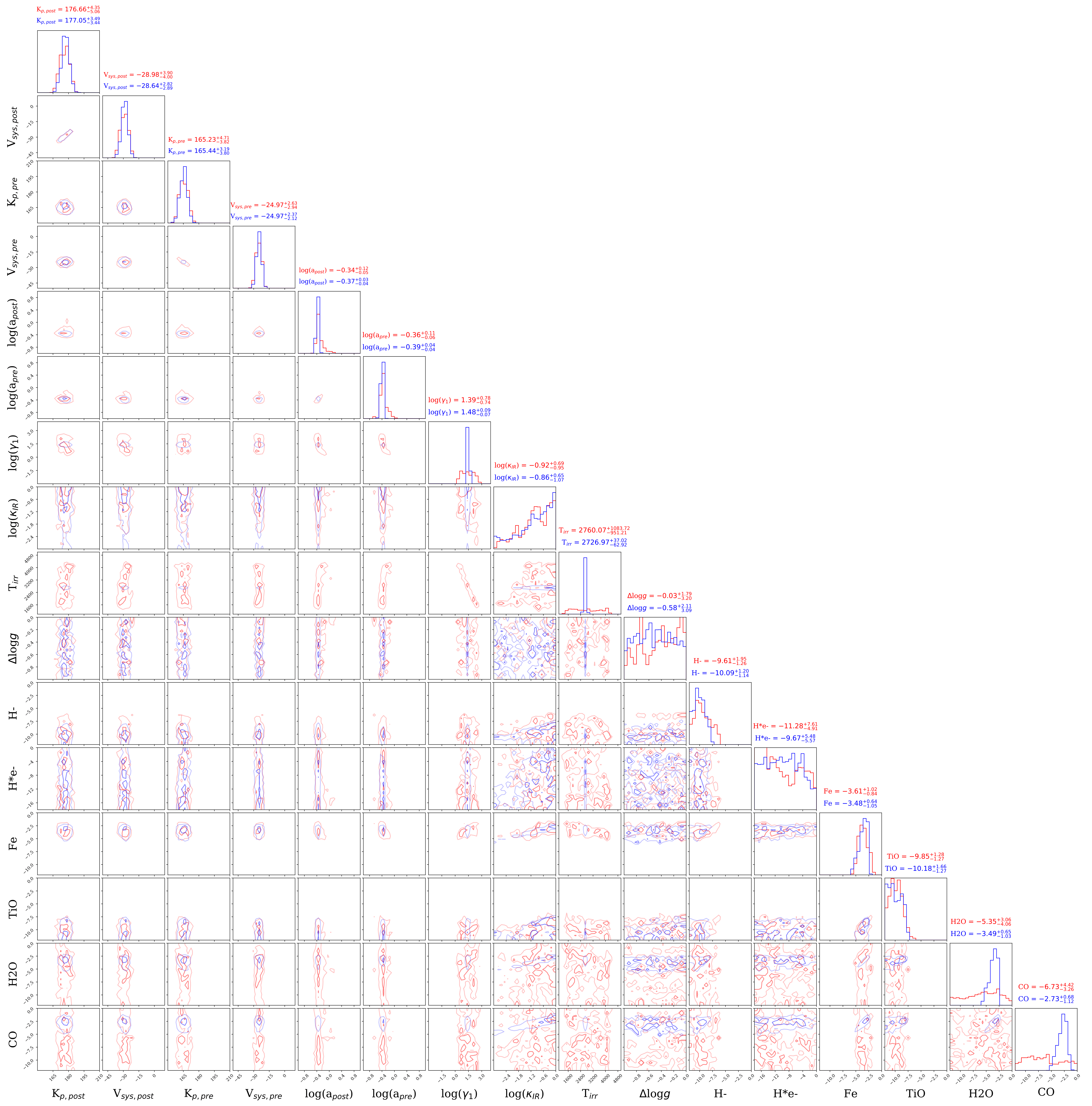
Figure 8: Full retrieval results for KELT-20b. Red indicates the retrieval on just the MAROON-X data (both channels and both nights together), and blue indicates the joint retrieval with the HST/WFC3 and Spitzer/IRAC data. The numerical values above each histogram panel are the median and 68% confidence interval. Both datasets by themselves provide sufficient evidence for the inversion. Isothermal atmospheres (i.e. log($\gamma_{1}$)=0) are strongly ruled out by the MAROON-X data alone as there is a hard edge to the log($\gamma_{1}$) in the MAROON-X Only data. There are no posterior samples below a log($\gamma_{1}$) value of 0.27 and this minimum value is excluded at $>$ 99.974%.

For our “MAROON-X only” retrieval we combined the blue and red arm MAROON-X data for both the pre- and post-eclipse observations. We also performed a joint retrieval on the combination of the MAROON-X observations and the HST/WFC3 and Spitzer/IRAC 4.5 $\mu$m observations presented in Fu et al. (2022). The joint retrieval was performed by combining the high-resolution and low-resolution likelihoods as described in Brogi & Line (2019). In all the retrievals we included H₂O, CO, TiO, Fe i, and abundance proxies for the H^- bound-free and free-free continua. The detection of Ni i occurred after we performed the retrieval analysis. Because the mass of the planet is not well constrained (upper limit of 3.5 M${}_{\text{Jup}}$, Lund et al., 2017), we also included a log $g$ free parameter that spanned a range between maximum log $g$ (3.28, cgs) and one dex below. The results are summarized in Figure 3 and the full corner plot is given in the Appendix (Figure 8). We note that in comparing the maximum log-likelihood difference between the two retrievals we found the difference as entirely due to the additional $red\chi^{2}\sim\,1$ data-points and that the MAROON-X contribution did not change in any meaningful way. This is unsurprising as there is little overlap in common parameters between the two datasets, with the exception of the T-P profile. E.g., water and CO do not present themselves in the MAROON-X data and the atomic species don’t show up in the WFC3. As relevant below, this suggests that any T-P profile information arising from the low-res contribution is fully consistent with what the MAROON-X data prefers.

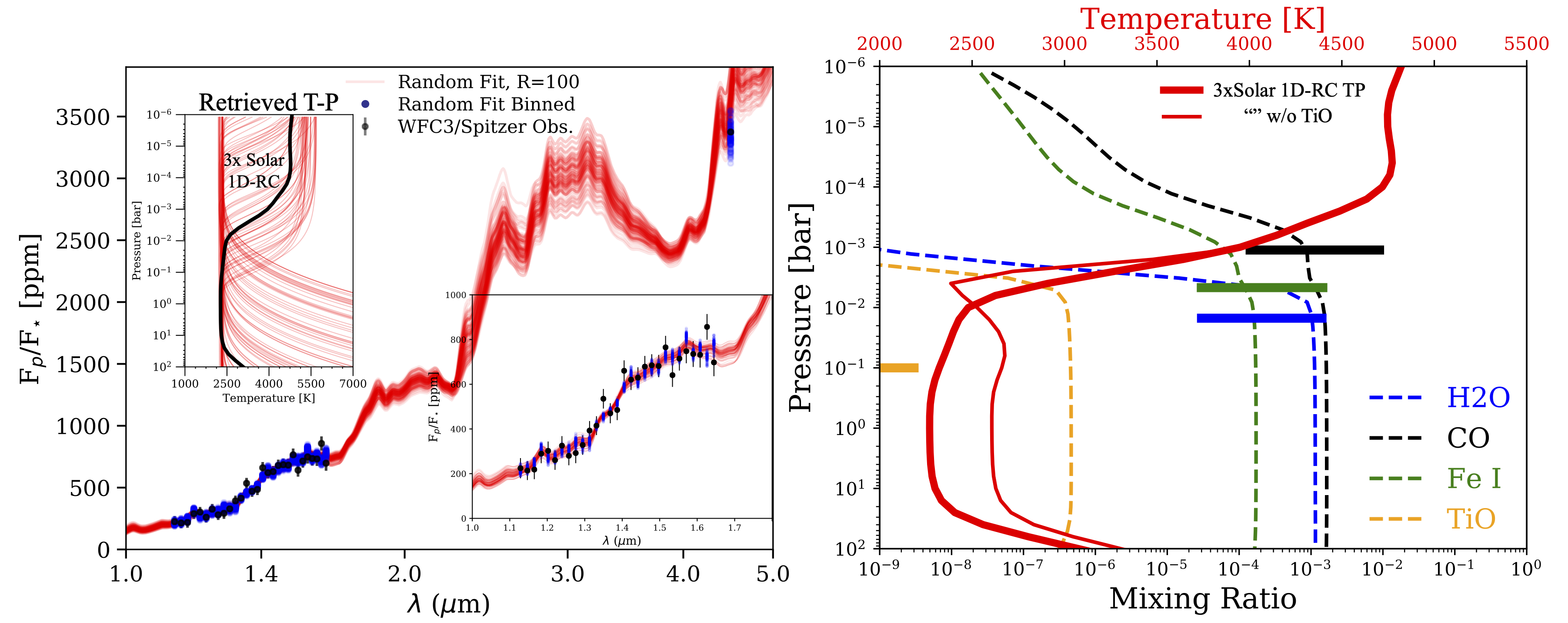
Figure 3: Summary of the joint retrieval analysis. The left panel shows the model fits to the space-based data resulting from the retrieval on the MAROON-X, HST/WFC3, and Spitzer/IRAC data. The red curves represent the spectra produced via 100 random draws from the posterior (smoothed to an R $=100$). The blue points are those same spectra binned to the WFC3 wavelengths. The smearing in the blue points illustrates the spread in the binned model spectra. The inset in the bottom right of the left panel shows a zoom in on the WFC3 data. The “Retrieved T-P” inset in the upper left shows reconstructed T-P profiles from 100 posterior draws from the combined MAROON-X, WFC3, and Spitzer (blue) observations. A $3\times$Solar 1D-RC model T-P profile from ScCHIMERA is shown in black for comparison. The right panel summarizes the retrieved abundance constraints in the context of a $3\times$solar 1D-RC model. The solid horizontal bars give the retrieved 68% confidence intervals on the chemical species. The position of the bars on the y axis (pressure axis) are at the approximate location probed by the wavelengths sensitive to those species (see Figure 9 in the appendix). The predicted thermochemical mixing ratio profiles are shown as dashed lines and the temperature profile is shown as the thick red curve (governed by the top x axis). The thinner red temperature profile is the same $3\times$solar scenario but with the opacity due to TiO/VO removed.

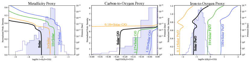
Figure 4: Comparison of retrieved elemental abundance proxies to those predicted from a battery of 1D-RC models. In each panel the histogram (scale on the left y-axis) is derived via a Monte Carlo propagation of the retrieved samples for Fe,i, H₂O, and CO into the quantity given under each x-axis (left: log(Fe i+H₂O+CO)), middle: log(CO/(H₂O+CO))), right: log(Fe i/(H₂O+CO))). The light shaded region is the 95% confidence interval for each proxy. The solid curves are the vertical abundance proxy profiles (pressure scale on the right y-axis of each panel) derived from the indicated 1D-RC models. In each panel, all elemental abundances are scaled uniformly by the indicated value relative to solar. The retrieved abundance proxy constraints are consistent with solar-composition, under the 1D-RC assumption.

The joint retrieval to all the datasets provides an excellent fit to the HST and Spitzer observations (median $\chi^{2}$ per number of data points is $\sim 0.9$, p-value=0.02). As expected from the results in the literature and the analysis in §3, the retrieval prefers a strong thermal inversion. The temperature gradient proxy parameter, log($\gamma_{1}$), is +21$\sigma$ away from zero, where a value of zero indicates an isothermal T-P profile, negative is a monotonically decreasing T-P profile, and positive is an inverted T-P profile (increasing temperature with decreasing pressure above the inversion level). The combined MAROON-X + HST and Spitzer retrieval provides a much more stringent constraint on this temperature gradient proxy than with MAROON-X alone (only 1.8$\sigma$ above zero, see blue vs. red histograms as well as additional caption details in Figure 8). We note that the pressure level at which the primary line forming temperature gradient resides is not well constrained [controlled by the log($\kappa_{IR}$) parameter] due to the lack of prior constraint on gravity and the degeneracy between metallicity and the “$\tau$=2/3” pressure level. In the top left inset on the left panel of Figure 3, this lack of constraint is apparent as the reconstructed T-P profiles invert at a continuum of pressure levels, with pressures below the inverted portion naturally becoming isothermal due to the Guillot (2010) profile parameterization employed, as it assumes a double gray formalism. The retrieved T-P profile gradient (as fully apparent in some reconstructions within the bounds of the figure) matches quite well the expectation from 1D-RC. However, this forward model includes TiO, which is seemingly absent given the data. We explore this issue more in the next section (§5).

The joint retrieval between the optical and near-to-mid IR enables constraints on both refractory (Fe) and volatile (C, O) elements. We derived bounded constraints on the abundances of Fe i, H₂O, and CO (Figure 8). The retrieved abundances are found to be in qualitative agreement with the expectations for a $\sim$3$\times$solar composition gas in thermochemical equilibrium (see the right panel of Figure 3). Inferring elemental abundance ratios from retrieved molecular abundances, especially with simplistic retrieval forward modeling assumptions, (e.g., constant-with-altitude volume mixing ratios) is not always straightforward [e.g., Sheppard et al. (2017) vs. Arcangeli et al. (2018)]. This is especially true in ultra-hot Jupiters where thermal dissociation can deplete the abundances of measurable species (e.g., Fe i, H₂O) into non-measured species (Fe ii, OH, O i). In order to place the retrieved abundances into context, we compare a series of elemental abundance proxies to a battery of, again, 1D-RC models, summarized in Figure 4.

We use the total sum of the bounded retrieved gases (Fe i+H₂O+CO) as a proxy for total metal enrichment (a.k.a, “metallicity”), the ratio, CO/(H₂O+CO) as a tracer of the carbon-to-oxygen ratio (C/O), and Fe i/(H₂O+CO) as a proxy for the iron-to-oxygen ratio (Fe/O). Figure 4 shows these secondary retrieval data-products as histograms compared to those same quantities (and their dependencies with altitude) from different composition 1D-RC models. We find that the overall metallicity (left most panel) is consistent with enrichment values $\lessapprox 30\times$solar, with a relatively loose lower bound of $\sim$0.1$\times$solar. Depending on the exact pressure level probed, the C/O (middle panel) can range anywhere between solar (C/O=0.55) to super-solar (C/O=0.85). Finally, we find the most stringent constraint on the Fe/O (right most panel). The retrieved values are largely consistent with solar, if not up to a few times solar (but below 10$\times$).

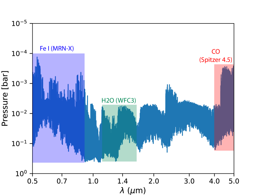
Figure 9: Pressure levels probed by the observations as dictated by the location of the $\tau=2/3$ level at each wavelength. As described in the text, the retrieval can’t precisely constrain the exact location of temperature with pressure due to the log($\kappa_{IR}$)-log$g$-metallicity degeneracy. Here, we show a representative surface from the 3$\times$solar 1D-RC model. The approximate pressure levels probed by each data-set by which species are indicated by the shaded boxes.

We can be more quantitative about the elemental abundance constraints if we make further assumptions about the pressure levels probed to correct for potential biases due to the constant-with-altitude gas mixing ratio assumption. As discussed above, we are unable to constrain the absolute pressure-level location of the base of the inversion. However, these degeneracies work out in such away that the $\tau$=2/3 level probed by the different wavelengths should always see the same temperature gradient, and largely the same abundance along a mixing ratio profile. An example of the pressure levels probed within the 3$\times$solar 1D-RC is shown in the Appendix ($\sim$0.1 bar to 0.1 mbar, see Figure 9).

Additionally, the constant-with-altitude gas mixing ratios assumed in the retrieval will be more heavily weighted towards the deeper, greater abundance layers, before molecular dissociation and atomic ionization occurs. Conveniently, our chosen elemental abundance proxies are fairly constant with pressure/altitude (within a 1D-RC) at layers deeper than the dissociation/ionization level (as also can be seen by the pressure levels probed in Figure 9). It is also true that in these deeper layers the C/O and Fe/O proxies are exact measures for those elemental ratios as Fe i, H₂O, and CO are the sole carriers of elemental Fe, O, and C (at altitudes where dissociation begins, O becomes predominately locked into OH and O i, in addition to CO, and Fe into Fe ii).

Given the above caveats and assumptions, we provide log of the abundances relative to the uniform regions of the solar composition 1D-RC model (thick black curves in each Figure 4 panel): [Fe i+H₂O+CO] = -1.28 – 1.49, [CO/(H₂O+CO)]=-0.47 – 0.19, and [Fe i/(H₂O+CO)] = -0.20 – 0.86 at 95% confidence (here “[X/Y]” is the usual bracket notation used for stellar abundances where zero is equal to solar). Taken together, the elemental abundance ratios are relatively unremarkable and largely consistent with solar-composition (perhaps a modest enhancement in the Fe/O and overall metallicity), and generally in-line with current trends (e.g. Kreidberg et al., 2014; Benneke, 2015) – any interpretation beyond that would not be supported by these data-sets.

The retrieval also provides an upper limit on the TiO volume mixing ratio of 10^-7.6 at 99% confidence. This is about one order of magnitude lower than the expectation from 3$\times$solar 1D-RC model. It has long been recognized that TiO could potentially play a major role in causing thermal inversions in hot Jupiter atmospheres (e.g., Hubeny et al., 2003; Fortney et al., 2008). However, detections of this species have been rare and not without controversy (see Prinoth et al., 2022, and references therein). KELT-20b has a strong thermal inversion, yet we and others have failed to find TiO in the emission spectrum (Yan et al., 2022a; Borsa et al., 2022; Johnson et al., 2022).

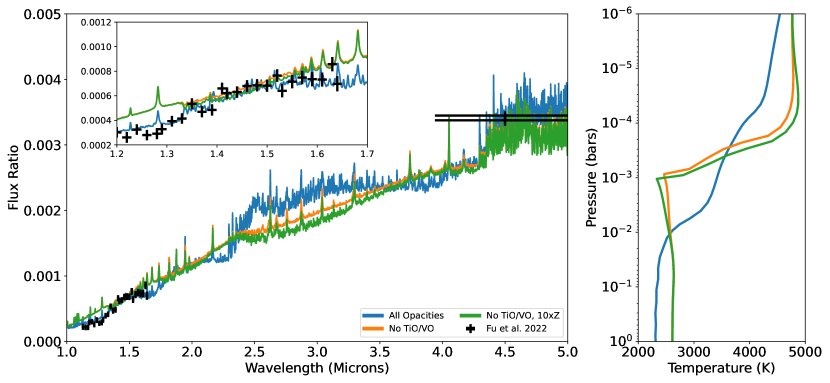
Figure 5: Secondary eclipse spectra (planet-to-star flux ratio, left) and T-P profiles (right) for KELT-20b from PHOENIX model calculations (lines) compared to the HST and Spitzer data of Fu et al. (2022, points). The inset zooms in on the HST/WFC3 data. The nominal model assuming thermochemical equilibrium for a solar composition gas is shown in blue. Models with TiO and VO opacity artificially removed are shown in orange (solar metallicity) and green ($10\times$ solar metallicity). The primary impact of this opacity is its influence on the thermal structure of the atmosphere rather than specific spectral features in the plotted region. The sharp emission lines in the spectra are a result of absorption lines expected in the stellar spectrum.

5 Radiative-Convective Equilibrium Atmosphere Models

The lack of TiO in the atmosphere of KELT-20b raises the question of what causes the strong thermal inversion. To explore this issue we modeled a number of scenarios with the PHOENIX 1D self-consistent radiative-convective equilibrium atmosphere model (Hauschildt et al., 1999; Barman et al., 2001). Our ultra-hot Jupiter model set-up was similar to those presented in Lothringer et al. (2018). We first modeled the atmosphere of KELT-20b with all available opacities, including atomic opacity from hydrogen up to uranium, continuous opacity sources like H^-, and molecular opacity, including TiO and VO. The resulting spectrum shows a qualitative match to the low-resolution HST and Spitzer observations of Fu et al. (2022), in agreement with the ScCHIMERA self-consistent models. However, we also computed a model without TiO and VO, since we do not find evidence of these species with our high-resolution observations. The results are summarized in Figure 5.

While the PHOENIX models with TiO and VO opacity artificially removed are a better match to the results of our (and others’) high-resolution observations, importantly, they do not match the low-resolution, space-based observations. This is due to the fact that without TiO and VO, the heating from the absorption of the short-wavelength stellar irradiation by species like the atomic metals is balanced by cooling by molecules like H₂O and CO. An inversion only forms at lower pressures once these latter molecules have thermally dissociated and can no longer radiatively cool the atmosphere. This means that the region that H₂O probes in the thermal emission spectrum is below the large temperature inversion and we would not expect to see H₂O in emission (see Figure 3). On the other hand, when TiO and VO are present, they can heat up the atmosphere in the region that H₂O probes, resulting in a strong H₂O emission feature. Thus, the non-detection of TiO and VO at high-resolution is in tension with the strong H₂O emission feature found by Fu et al. (2022).

Lothringer & Barman (2019) pointed out the importance of the host star spectral energy distribution in setting the thermal structure of highly irradiated planets. Fu et al. (2022) suggested that KELT-20b’s A-type host star, with its higher proportion of short-wavelength flux than the typical hot Jupiter host star, is likely responsible for the large water emission feature seen in the planet’s spectrum. Therefore, if TiO is not present to cause the thermal inversion at the deep pressures where H₂O is still intact then it could be that the models are missing opacity at the short wavelengths where the host star is particularly bright.

6 Discussion

Our detection of atomic emission lines agrees with the broad conclusions of recent publications analyzing the dayside of the ultra-Hot Jupiter KELT-20b: there is a thermal inversion in the atmosphere and neutral iron (as opposed to TiO or VO) is the dominant optical opacity source observed in the spectrum (Borsa et al., 2022; Yan et al., 2022a; Johnson et al., 2022). Additionally, for the first time with KELT-20b we search for and find Ni i (at 4.7$\sigma$ confidence).

KELT-20b is one of the coolest exoplanets known to have a thermal inversion and it has the strongest water emission feature seen in over two dozen hot Jupiter emission spectra obtained with HST/WFC3 (Fu et al., 2022). However, there have been no detections of TiO or atomic Ti in either its emission spectrum or in the many observations of its transmission spectrum (Bello-Arufe et al., 2022; Langeveld et al., 2022; Rainer et al., 2021; Nugroho et al., 2020; Stangret et al., 2020; Hoeijmakers et al., 2020; Kesseli et al., 2020; Casasayas-Barris et al., 2019). Given the presence of the other refractory species that have been detected for this planet (in addition to those described already, Na, Mg, Ca, and Cr species have also been detected in the transmission spectrum), sequestration of Ti in the unobservable parts of the atmosphere due to cold trapping seems a likely explanation (Spiegel et al., 2009; Parmentier et al., 2013). Intriguingly, models with TiO cold trapping can also fit the ensemble of WFC3 spectra (see Figure 4 in Mansfield et al., 2021). This fact combined with the rarity of TiO detections suggests that cold-trapping of Ti might be a common phenomenon in hot and ultra-hot Jupiter atmospheres. More work is needed to explore this emerging population-level trend.

Lothringer et al. (2021) have proposed that the ratio of refractory and volatile species abundances is an important tracer of planet formation. KELT-20b is one of the few planets where Fe, H₂O, and CO spectral features are present in the thermal emission spectrum. The thermal emission spectrum typically arises from deeper atmospheric layers than the transmission spectrum, which can probe such high altitudes that mass fractionation of different chemical species can be an issue, thus complicating the interpretation of abundance measurements. By exhibiting Fe, H₂O, and CO features that arise from the bulk atmosphere, KELT-20b in principle presents an important opportunity to connect Fe/O and Fe/C abundance ratios to models of giant planet formation.

We have constrained the abundances of Fe i, H₂O, and CO for KELT-20b by performing a unified retrieval on ground-based, high-resolution optical spectroscopy and space-based low-resolution infrared spectroscopy. This extends our previous work by Brogi et al. (2017), which only conditioned an analysis of high-resolution data on a low-resolution retrieval, and the work of Brogi & Line (2019), which developed our joint retrieval framework on simulated data. To our knowledge only one other such retrieval has been performed on real data before, by Gandhi et al. (2019).

Our measured Fe i, H₂O, and CO abundances and their ratios are consistent with a solar elemental Fe, C, and O under the assumption of 1D radiative-convective-thermochemical equilibrium. Further observations of KELT-20b could build on this work to determine more precise abundances of these elements as a constraint on the planet’s formation. Of particular value would be a measurement of the mass of the planet, broader wavelength space-based spectroscopy from the James Webb Space Telescope, and ground-based observations to probe the H₂O and CO lines at higher spectral resolution (e.g., Line et al., 2021; Pelletier et al., 2021; van Sluijs et al., 2022; Yan et al., 2022b; Holmberg & Madhusudhan, 2022). In addition, advances in retrieval techniques are needed to ensure that the derived abundances are also accurate. A key limitation of the current state-of-the-art retrievals applied to high-resolution spectroscopy is the predominant assumption of 1D atmospheres and constant-with-altitude abundances. Future work that incorporates variations of temperature and abundance with longitude and altitude (e.g. Gandhi et al., 2022) will be critical to ensuring valid composition inferences as we continue to push towards higher fidelity datasets.

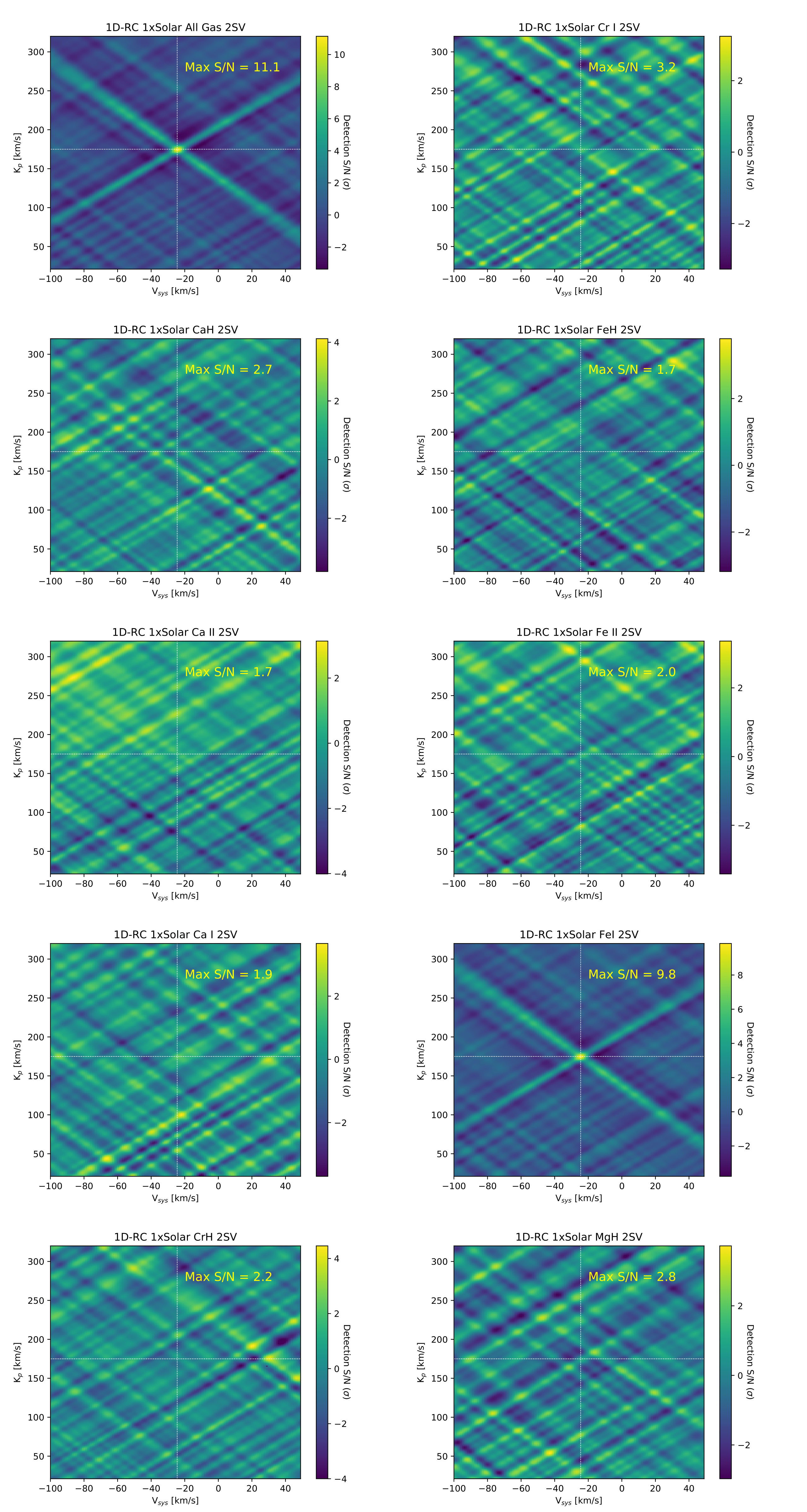
Figure 6: Maps of the CCF in the planet velocity ($K_{p}$) vs. system velocity ($V_{\text{sys}}$) plane using the combined dataset and all 1D-RC model spectra explored (as labeled above each map). Dotted lines correspond to the known system velocity and exoplanet orbital speed of -24.5 km s^-1 and 175 km s^-1, respectively, as in Borsa et al. (2022). Continued below.

Figure 7: Continuation of Fig 6

References

- Arcangeli et al. (2018) Arcangeli, J., Désert, J.-M., Line, M. R., et al. 2018, ApJ, 855, L30, doi: 10.3847/2041-8213/aab272
- Astropy Collaboration et al. (2018) Astropy Collaboration, Price-Whelan, A. M., Sipőcz, B. M., et al. 2018, AJ, 156, 123, doi: 10.3847/1538-3881/aabc4f
- Barman et al. (2001) Barman, T. S., Hauschildt, P. H., & Allard, F. 2001, ApJ, 556, 885, doi: 10.1086/321610
- Bello-Arufe et al. (2022) Bello-Arufe, A., Buchhave, L. A., Mendonça, J. M., et al. 2022, arXiv e-prints, arXiv:2203.04969. https://arxiv.org/abs/2203.04969
- Benneke (2015) Benneke, B. 2015, ArXiv e-prints: 1504.07655. https://arxiv.org/abs/1504.07655
- Bernath (2020) Bernath, P. F. 2020, J. Quant. Spec. Radiat. Transf., 240, 106687, doi: https://doi.org/10.1016/j.jqsrt.2019.106687
- Borsa et al. (2022) Borsa, F., Giacobbe, P., Bonomo, A. S., et al. 2022, arXiv e-prints, arXiv:2204.04948. https://arxiv.org/abs/2204.04948
- Brogi et al. (2017) Brogi, M., Line, M., Bean, J., Désert, J.-M., & Schwarz, H. 2017, ApJ, 839, L2, doi: 10.3847/2041-8213/aa6933
- Brogi & Line (2019) Brogi, M., & Line, M. R. 2019, AJ, 157, 114
- Casasayas-Barris et al. (2019) Casasayas-Barris, N., Pallé, E., Yan, F., et al. 2019, A&A, 628, A9, doi: 10.1051/0004-6361/201935623
- Foreman-Mackey (2016) Foreman-Mackey, D. 2016, The Journal of Open Source Software, 1, 24, doi: 10.21105/joss.00024
- Fortney et al. (2008) Fortney, J. J., Lodders, K., Marley, M. S., & Freedman, R. S. 2008, ApJ, 678, 1419, doi: 10.1086/528370
- Fu et al. (2022) Fu, G., Sing, D. K., Lothringer, J. D., et al. 2022, ApJ, 925, L3, doi: 10.3847/2041-8213/ac4968
- Gandhi et al. (2022) Gandhi, S., Kesseli, A., Snellen, I., et al. 2022, MNRAS, doi: 10.1093/mnras/stac1744
- Gandhi et al. (2019) Gandhi, S., Madhusudhan, N., Hawker, G., & Piette, A. 2019, AJ, 158, 228, doi: 10.3847/1538-3881/ab4efc
- Gharib-Nezhad et al. (2021) Gharib-Nezhad, E., Iyer, A. R., Line, M. R., et al. 2021, ApJS, 254, 34, doi: 10.3847/1538-4365/abf504
- GharibNezhad et al. (2013) GharibNezhad, E., Shayesteh, A., & Bernath, P. F. 2013, MNRAS, 432, 2043, doi: 10.1093/mnras/stt510
- Giacobbe et al. (2021) Giacobbe, P., Brogi, M., Gandhi, S., et al. 2021, Nature, 592, 205, doi: 10.1038/s41586-021-03381-x
- Grimm & Heng (2015) Grimm, S. L., & Heng, K. 2015, ApJ, 808, 182, doi: 10.1088/0004-637X/808/2/182
- Grimm et al. (2021) Grimm, S. L., Malik, M., Kitzmann, D., et al. 2021, ApJS, 253, 30, doi: 10.3847/1538-4365/abd773
- Guillot (2010) Guillot, T. 2010, A&A, 520, A27+, doi: 10.1051/0004-6361/200913396
- Harris et al. (2020) Harris, C. R., Millman, K. J., van der Walt, S. J., et al. 2020, Nature, 585, 357, doi: 10.1038/s41586-020-2649-2
- Hauschildt et al. (1999) Hauschildt, P. H., Allard, F., & Baron, E. 1999, ApJ, 512, 377, doi: 10.1086/306745
- Hoeijmakers et al. (2020) Hoeijmakers, H. J., Cabot, S. H. C., Zhao, L., et al. 2020, A&A, 641, A120, doi: 10.1051/0004-6361/202037437
- Holmberg & Madhusudhan (2022) Holmberg, M., & Madhusudhan, N. 2022, arXiv e-prints, arXiv:2206.10621. https://arxiv.org/abs/2206.10621
- Hubeny et al. (2003) Hubeny, I., Burrows, A., & Sudarsky, D. 2003, ApJ, 594, 1011, doi: 10.1086/377080
- Hunter (2007) Hunter, J. D. 2007, Computing in Science & Engineering, 9, 90, doi: 10.1109/MCSE.2007.55
- John (1988) John, T. L. 1988, A&A, 193, 189
- Johnson et al. (2022) Johnson, M. C., Wang, J., Pai Asnodkar, A., et al. 2022, arXiv e-prints, arXiv:2205.12162. https://arxiv.org/abs/2205.12162
- Kanodia & Wright (2018) Kanodia, S., & Wright, J. 2018, Research Notes of the AAS, 2, 4, doi: 10.3847/2515-5172/aaa4b7
- Kasper et al. (2021) Kasper, D., Bean, J. L., Line, M. R., et al. 2021, ApJ, 921, L18, doi: 10.3847/2041-8213/ac30e1
- Kesseli et al. (2020) Kesseli, A. Y., Snellen, I. A. G., Alonso-Floriano, F. J., Mollière, P., & Serindag, D. B. 2020, AJ, 160, 228, doi: 10.3847/1538-3881/abb59c
- Kreidberg et al. (2014) Kreidberg, L., Bean, J. L., Désert, J.-M., et al. 2014, Nature, 505, 69, doi: 10.1038/nature12888
- Langeveld et al. (2022) Langeveld, A. B., Madhusudhan, N., & Cabot, S. H. C. 2022, arXiv e-prints, arXiv:2205.01623. https://arxiv.org/abs/2205.01623
- Line et al. (2021) Line, M. R., Brogi, M., Bean, J. L., et al. 2021, Nature, 598, 580, doi: 10.1038/s41586-021-03912-6