Multipartite Nonlocality in Clifford Networks
Abstract
We adopt a resource-theoretic framework to classify different types of quantum network nonlocality in terms of operational constraints placed on the network. One type of constraint limits the parties to perform local Clifford gates on pure stabilizer states, and we show that quantum network nonlocality cannot emerge in this setting. Yet, if the constraint is relaxed to allow for mixed stabilizer states, then network nonlocality can indeed be obtained. We additionally show that bipartite entanglement is sufficient for generating all forms of quantum network nonlocality when allowing for post-selection, a property analogous to the universality of bipartite entanglement for generating all forms of multipartite entangled states.
The Gottesman-Knill Theorem is a classic result that enables a wide class of quantum algorithms to be efficiently simulated [1, 2, 3]. It says that circuits constructed using only gates belonging to the Clifford group can be efficiently simulated on a classical computer using the stabilizer formalism. It is interesting to investigate whether Clifford quantum information processing has similar limitations for other quantum information tasks and phenomena, such as the emergence of quantum nonlocality. It has already been shown [4, 5, 6, 7] that such limitations do indeed exist in specific scenarios, but the role of Clifford operations in the emergence of network nonlocality has remained relatively unexplored.
The standard Bell nonlocality scenario consists of multiple parties having access to some globally-shared entangled state, and they each select different measurements to perform on their respective subsystems [8]. In the network setting, the globally-shared entanglement is replaced by independent sources of entanglement that get distributed according to the structure of the network [9, 10, 11, 12, 13]. Examples of nonlocality in networks have recently been found that appear to be fundamentally different than the nonlocality emerging in traditional Bell scenarios [14, 15, 16, 17, 18, 19], although how to best articulate this difference is unclear.
To shed light on this question, we begin here by sketching a “top-down” framework for the general study of quantum nonlocality (or “nonclassicality”), inspired by the philosophy of quantum resource theories [20, 21]. In this framework, different classes of nonlocality naturally emerge on a quantum network after placing different restrictions on the type of states that are “free” to distribute across the network, as well as the type of local operations that the parties are free to perform. This allows us to view different notions of nonlocality proposed in the literature under a common conceptual lens. As our main result, we show later in this letter that quantum nonlocality can never be realized whenever the parties are restricted to Clifford operations and the free states are stabilizer states.
An operational framework for network nonlocality.
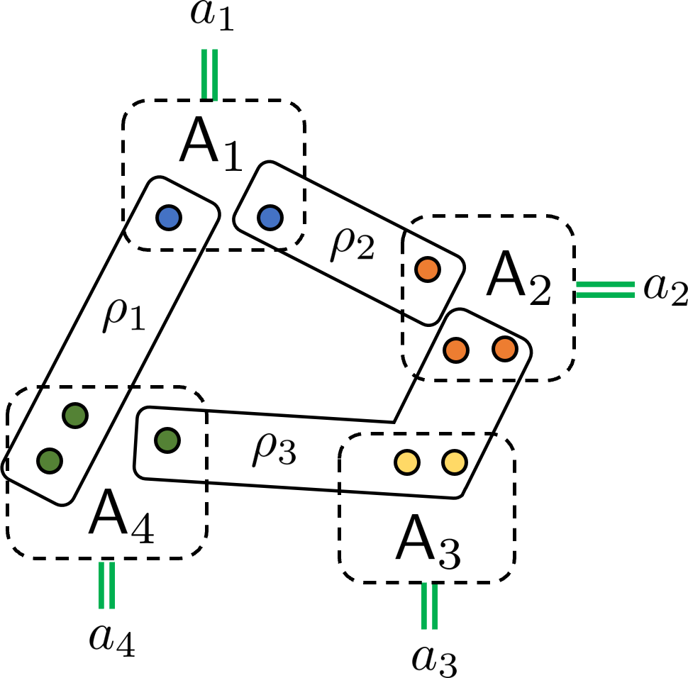
Consider an -party quantum network whose structure is defined by a hypergraph with a disjoint hyperedge set . Each vertex represents a quantum system, and each hyperedge represents an independent quantum source that generates a joint state for all systems in . The network structure also specifies which quantum systems are received locally by each party. We let denote the collection of hyperedges connected to party (see Fig. 1). In any protocol for generating network correlations, each party applies a quantum channel jointly across all its received systems, thereby connecting the previously disjoint hyperedges. The parties then measure their systems in the computational basis, and the collective output is the -tuple of measured values with probability distribution . In summary, every network correlation we consider can be generated using the following three-step procedure:
-
(i)
For each hyperedge in the network, a multipartite state is distributed across the network;
-
(ii)
Each party performs a local processing channel on the systems under its control;
-
(iii)
Each party measures its post-processed system in the computational basis and outputs the outcome .
A distribution built in this way will be called a quantum network correlation.
Since this framework is designed to study quantum nonlocality, one may want to generalize the setup and grant each party an input variable that controls the local processing performed. In this case, the generated correlation would be a conditional distribution , which is typically the object of consideration in the study of Bell nonlocality. However, in the network scenario, the distinction between correlations with inputs versus correlations without inputs is superficial. This is due to the work of Fritz [22], who showed how every correlation generated on some network with inputs can be equivalently generated on an enlarged network without inputs; essentially the local input variable of party becomes an independent variable shared between and some new party on the enlarged network. Therefore, without loss of generality, we restrict to correlations with no inputs.
With this model in place, we can now identify different classes of quantum correlations by imposing different constraints on the distributed states and the types of local maps . We begin with the set of local correlations defined with respect to a given network . A network local correlation is any distribution that can be generated using a shared classical variable for each hyperedge . If denotes the probability distribution over variable , then every local correlation has the form
| (1) |
where the sum is over each sequence of the independent random variables, , and is a local classical channel of party . If a quantum network correlation does not have this form, then it is called quantum network nonlocal. We claim that the set of local correlations is precisely those that can be generated via steps (i)–(iii) above under the constraint that each satisfies the condition
| (2) |
where is the completely dephasing map in the computational basis. This condition has previously been called resource non-activating [23], but in this work we will say that any completely-positive trace-preserving (CPTP) map satisfying Eq. (2) is classically simulatable. Indeed, any correlation generated using classically simultable maps can be simulated on the same network using purely classical resources. Since the parties measure their qubits in the computational basis after applying in step (ii), Eq. (2) says that the parties could equivalently also dephase the shared state prior to step (ii), thereby converting each into a classically correlated state , where . Conversely, any network correlation generated using classical shared randomness can also be produced using classically correlated states and CPTP maps of the form , where
| Operational constraint | Inaccessible type of network correlation |
| are classically simultable | Network nonlocality |
| are local quantum wiring maps | Genuine network nonlocality [24] |
| are classically simultable for at least one party in a given subgraph | Full network nonlocality for the given subgraph [18] |
| are Clifford gates and are pure stabilizer states | Network nonlocality |
Another type of constraint limits each to be a local quantum wiring map for party [25, 26, 24], which can be understood as a local operations and classical communication (LOCC) transformation performed on the separated systems that receives from different sources. Under this constraint, is prohibited from performing entangling measurements across the different states it receives, such as in entanglement swapping. Nevertheless, these operations are still strong enough to generate nonlocal correlations when seeded with at least one entangled state on the network. All “standard” Bell tests - such as the celebrated violations of the Clauser-Horne-Shimony-Holt (CHSH) inequality [27, 28, 29] - can be implemented under the restriction of local quantum wiring maps. In contrast, network correlations not producible by local quantum wiring maps can be defined as possessing genuine network nonlocality [24], much in the same way that quantum states not producible by LOCC are defined as possessing entanglement [30]. This definition is motivated by the fact that to produce genuine quantum network nonlocality, the parties must be able to truly leverage the network structure and stitch together the different quantum sources through non-classical local interactions.
To provide a complete account of the different notions of network nonlocality proposed in the literature, we consider one final type of correlation. For a fixed subgraph of a given network, one could require that at least one of the constituent parties performs a classically simulatable operation . Nonlocal correlations that cannot generated under this restriction are said to possess full network nonlocality with respect to the particular subgraph [18].
We now enjoin the main result of this letter to the picture. Let be any quantum network correlation built under the constraint that all are pure stabilizer states and the are Clifford gates. Then is a network local distribution. The rest of this letter will be devoted to explaining this result and its proof in more detail; technical steps are postponed to the Supplemental Material. Table 1 summarizes the different types of network correlations in the context of the operational framework outlined above.
-network nonlocality. Before specializing to Clifford networks, let us first sharpen the notion of local correlations to reflect even better the structure of the network. Let us say that a -network is any hypergraph with disjoint edge set in which every quantum source is connected to no more than parties; i.e. for all . An -party distribution that can be built using classically simulatable operations on some -network will be called -network local; otherwise it will be called quantum -network nonlocal.
It turns out that every instance of quantum -network nonlocality can be obtained from a quantum -network nonlocal correlation through post-selection.
Proposition 1.
Suppose that is a quantum -network nonlocal correlation for parties. Then there exists an -party correlation that is quantum -network nonlocal and satisfies
| (3) |
In other words, conditioned on the new parties having the all-zero output, the other parties reproduce the original distribution .
To prove this proposition one replaces every -element hyperedge with bipartite edges and then uses bipartite entanglement distributed on these edges to teleport the original state . We remark that our reduction to -network nonlocality from -network nonlocality via post-selection is specific to quantum networks, as it relies on quantum teleportation. It is an interesting question whether such a reduction can be found for general non-signaling network correlations [31, 32] or whether this is a uniquely quantum feature.
Clifford Networks. Let us now turn to the notion of Clifford quantum networks, which can be understood as distributed Clifford circuits [1]. We begin by recalling the definitions of stabilizers and stabilizer operations [33, 1, 34]. Let denote the -qubit Pauli group of operators, . Expressions like express Pauli- applied to qubit and the identity applied to all other qubits. The -qubit Clifford group consists of all unitaries that, up to an overall phase, leave invariant under conjugation,
| (4) |
The set of -qubit stabilizer states is defined as
| (5) |
Every stabilizer pure state can be uniquely identified as the eigenstate of independent commuting elements from . These operators generate a group, called a stabilizer group, that we denote by .
Consider now a -network in which each vertex represents a qubit system. The hyperedges again form a disjoint partitioning of the vertex set and each represents a multi-qubit state. Suppose that party receives a total of qubits from the various sources. Using the three-step framework introduced above, we consider correlations formed under the following restrictions:
-
(ic)
For each hyperedge , a pure stabilizer state is distributed;
-
(iic)
Each party introduces ancilla qubits, each initialized in state , and performs a Clifford unitary gate on all the qubits held locally.
Like before, step (iii) involves a measurement of each qubit in the computational basis. This generates a classical output for each party that is a sequence of bits , one for each qubit used by party in the protocol. Letting and , the joint probability distribution for all measurements is then given by
| (6) |
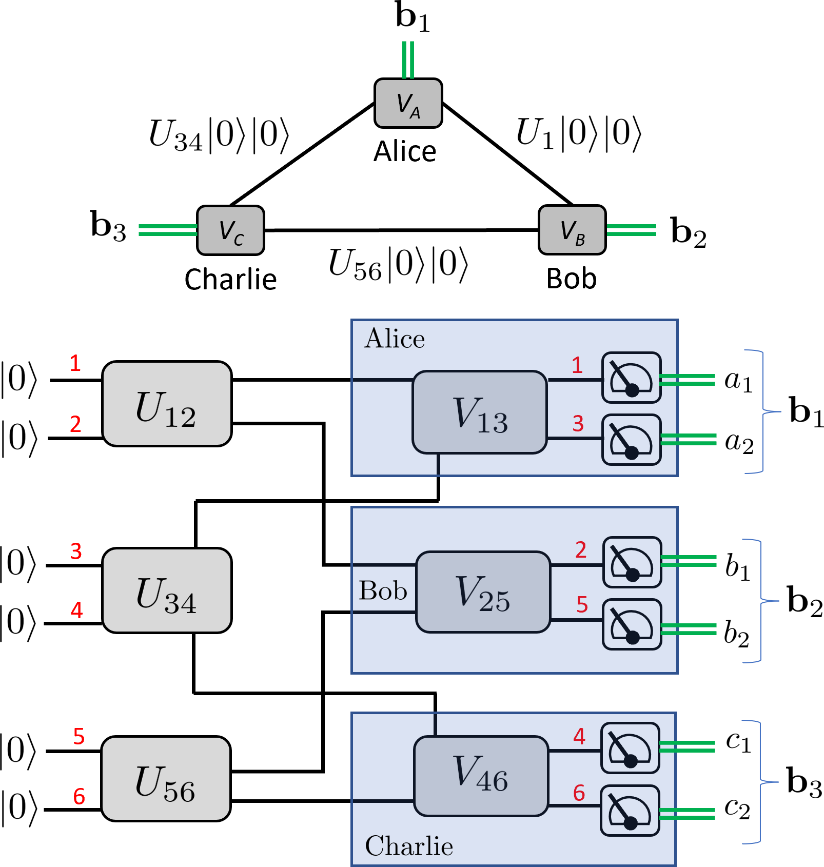
Every distribution having this form will be called a Clifford -network correlation. As an example, a triangle Clifford network is depicted in Fig. 2. Its equivalent representation as a distributed quantum circuit is also shown.
Observe that the Clifford constraint and the classical simulatable constraint are inequivalent; i.e., there are Clifford gates (such as Hadamard) whose corresponding CPTP map fails to satisfy Eq. (2) and vice-versa. Yet, on the level of network nonlocality, our result shows that Clifford operations fail to offer any non-classical advantage.
Theorem 1.
Every Clifford -network correlation is -network local.
The proof of this theorem begins by performing three simplifications. First, in Proposition 1 we established that every quantum -network nonlocal distribution can be obtained from a quantum -network nonlocal distribution via post-selection. Moreover, since teleportation is carried out using Pauli gates, the proof of Proposition 1 can be specialized to Clifford networks: if a quantum -network nonlocal distribution is generated on a Clifford -network, then there exists a quantum -network nonlocal distribution generated on a Clifford -network. Hence, to prove Theorem 1, it suffices to show that measuring Clifford -network states always leads to -network local distributions. In other words, we can restrict to just being a graph so that each is a bipartite stabilizer state. Second, recall the fact that every bipartite stabilizer state can be transformed into copies of and computational basis states using local Cliffords [35]. Third, as proved in the Supplemental Material, the use of local ancilla provides no advantage for the purpose of generating -network nonlocality. Then it suffices to consider graphs in which each node is connected to exactly one other node, the two nodes are held by different parties, and their connecting edge represents a maximally entangled state shared between them.
The next part of the proof involves constructing a local model for any graph having this structure and any choice of local stabilizer measurement. Our local model involves replacing each edge on the graph with a random variable , which is a trio of uniform independent random bits. Based on the local measurement wants to perform and the values , outputs can be generated that jointly have the correct distribution . Details of the model and a proof of its correctness are presented in the Supplemental Material. During the completion of this manuscript we became aware of a similar model independently derived by Matthew Pusey in Ref. [4], although it does not directly account for network constraints and the emergence of network nonlocality 111One feature of Pusey’s model in Ref. [4] that can also be applied here is a slight simplification of the shared classical randomness. Instead of needing a trio of random bits for each edge , it suffices to have two bits and then compute the third random bit as their product, ..
Discussion. In this letter, we have presented a unifying framework for the general study of quantum network nonlocality. We believe this framework can help clarify what types of quantum resources are needed to generate different forms of nonlocality. It also helps draw a trifold connection between nonlocality, quantum resource theories, and quantum computation, as shown in Fig. 2. When any protocol is fully decomposed as a distributed quantum circuit, we found that some non-Clifford operation is needed to generate nonlocal correlations.
The importance of non-Clifford operations is further corroborated by the purported examples of genuine network nonlocality or full network nonlocality found in the literature [14, 15, 16, 17, 18, 19]. In each of these examples some non-Clifford operation is needed to realize the nonlocality. Even more conspicuously, in the triangle network considered by Renou et al. in Ref. [14], nonlocality fails to emerge exactly when the parameters of their model coincided with a Clifford network. Our work formalizes the reason why this happens, and can thus be interpreted as a guide for what kind of resources are needed to generate network nonlocality.
One may feel that Theorem 1 is not that surprising given the Gottesman-Knill Theorem for simulating Clifford circuits. However, let us highlight two reasons why the former stands independently of the latter, despite them sharing a kindred spirit. First, the Gottesman-Knill Theorem provides a classical algorithm to correctly reproduce the outcome statistics when locally measuring a stabilizer state. However, in this algorithm, one must update the generators of the stabilizer after simulating the measurement of each qubit. This requires the communication of global information, which is forbidden in the network nonlocality model. Therefore, a completely new classical model is needed for a distributed simulation, which is what Theorem 1 provides.
Second, Theorem 1 breaks down when relaxing certain operational restrictions whereas the Gottesman-Knill Theorem does not. Specifically, suppose we relax condition (ic) by allowing for mixed stabilizer states; i.e. convex combinations of stabilizer states whose purification is no longer a stabilizer state. Remarkably, now it becomes possible to violate Theorem 1 using so-called “disguised” Bell nonlocality [13]. The construction is presented in the Supplemental Material and involves extending Mermin’s magic square game [37] to the network setting using a slight modification of Fritz’s construction. This result highlights the strong non-convexity that emerges in network nonlocality: local models can be constructed for all pure stabilizer states, but this fails to be possible when taking their mixture. It is tempting to think that the classical randomness in the mixed state could just be absorbed into the classical randomness distributed on edge . However, this does not always work since the local classical strategy for some party in simulating a Clifford network distribution might depend on which state is seeded on edge , even if is not connected on .
Similarly, one could consider relaxing condition (iic) by allowing for convex combinations of Clifford gates; i.e. with each being a Clifford. Then by a similar construction to the one used for mixed stabilizer states, it is is possible to generate nonlocality on the network. The problem is that not every Clifford channel like admits a unitary diltation that itself is Clifford, and thus Theorem 1 does not apply. In contrast, the Gottesman-Knill Theorem still provides an efficient classical simulation algorithm for quantum circuits using mixed stabilizer states and random Clifford channels [38]. Ultimately, we hope that these findings and the framework described here help pinpoint the precise conditions necessary for generating nonlocal correlations on a quantum network.
Acknowledgments – We thank Marc-Olivier Renou for discussing with us the subtleties of disguised network nonlocality. We are also grateful to Mark Howard, Jonathan Barrett, Nicolas Brunner, and Matthew Pusey for bringing several precursor works to our attention and discussing other connections between Clifford circuits and local classical models. This material is based upon work supported by the U.S. Department of Energy Office of Science National Quantum Information Science Research Centers.
References
- Gottesman [1998] D. Gottesman, The heisenberg representation of quantum computers (1998), arXiv:quant-ph/9807006 .
- Aaronson and Gottesman [2004] S. Aaronson and D. Gottesman, Improved simulation of stabilizer circuits, Phys. Rev. A 70, 052328 (2004).
- Anders and Briegel [2006] S. Anders and H. J. Briegel, Fast simulation of stabilizer circuits using a graph-state representation, Phys. Rev. A 73, 022334 (2006).
- Pusey [2010] M. Pusey, A few connections between Quantum Computation and Quantum Non-Locality, Master’s thesis, Imperial College London (2010).
- Tessier et al. [2005] T. E. Tessier, C. M. Caves, I. H. Deutsch, B. Eastin, and D. Bacon, Optimal classical-communication-assisted local model of -qubit greenberger-horne-zeilinger correlations, Phys. Rev. A 72, 032305 (2005).
- Howard and Vala [2012] M. Howard and J. Vala, Nonlocality as a benchmark for universal quantum computation in ising anyon topological quantum computers, Phys. Rev. A 85, 022304 (2012).
- Howard [2015] M. Howard, Maximum nonlocality and minimum uncertainty using magic states, Phys. Rev. A 91, 042103 (2015).
- Brunner et al. [2014] N. Brunner, D. Cavalcanti, S. Pironio, V. Scarani, and S. Wehner, Bell nonlocality, Rev. Mod. Phys. 86, 419 (2014).
- Branciard et al. [2010] C. Branciard, N. Gisin, and S. Pironio, Characterizing the nonlocal correlations created via entanglement swapping, Phys. Rev. Lett. 104, 170401 (2010).
- Bancal et al. [2011] J.-D. Bancal, N. Brunner, N. Gisin, and Y.-C. Liang, Detecting genuine multipartite quantum nonlocality: A simple approach and generalization to arbitrary dimensions, Phys. Rev. Lett. 106, 020405 (2011).
- Branciard et al. [2012] C. Branciard, D. Rosset, N. Gisin, and S. Pironio, Bilocal versus nonbilocal correlations in entanglement-swapping experiments, Phys. Rev. A 85, 032119 (2012).
- Gisin [2019] N. Gisin, Entanglement 25 years after quantum teleportation: Testing joint measurements in quantum networks, Entropy 21, 325 (2019).
- Tavakoli et al. [2022] A. Tavakoli, A. Pozas-Kerstjens, M.-X. Luo, and M.-O. Renou, Bell nonlocality in networks, Reports on Progress in Physics 85, 056001 (2022).
- Renou et al. [2019] M.-O. Renou, E. Bäumer, S. Boreiri, N. Brunner, N. Gisin, and S. Beigi, Genuine quantum nonlocality in the triangle network, Phys. Rev. Lett. 123, 140401 (2019).
- Tavakoli et al. [2021] A. Tavakoli, N. Gisin, and C. Branciard, Bilocal bell inequalities violated by the quantum elegant joint measurement, Phys. Rev. Lett. 126, 220401 (2021).
- Renou and Beigi [2022a] M.-O. Renou and S. Beigi, Network nonlocality via rigidity of token counting and color matching, Phys. Rev. A 105, 022408 (2022a).
- Renou and Beigi [2022b] M.-O. Renou and S. Beigi, Nonlocality for generic networks, Phys. Rev. Lett. 128, 060401 (2022b).
- Pozas-Kerstjens et al. [2022a] A. Pozas-Kerstjens, N. Gisin, and A. Tavakoli, Full network nonlocality, Phys. Rev. Lett. 128, 010403 (2022a).
- Pozas-Kerstjens et al. [2022b] A. Pozas-Kerstjens, N. Gisin, and M.-O. Renou, Proofs of network quantum nonlocality aided by machine learning (2022b), arXiv:2203.16543 .
- Horodecki and Oppenheim [2012] M. Horodecki and J. Oppenheim, (quantumness in the context of) resource theories, International Journal of Modern Physics B 27, 1345019 (2012).
- Chitambar and Gour [2019] E. Chitambar and G. Gour, Quantum resource theories, Rev. Mod. Phys. 91, 025001 (2019).
- Fritz [2012] T. Fritz, Beyond bell’s theorem: correlation scenarios, New Journal of Physics 14, 103001 (2012).
- Liu et al. [2017] Z.-W. Liu, X. Hu, and S. Lloyd, Resource destroying maps, Phys. Rev. Lett. 118, 060502 (2017).
- Šupić et al. [2022] I. Šupić, J.-D. Bancal, Y. Cai, and N. Brunner, Genuine network quantum nonlocality and self-testing, Phys. Rev. A 105, 022206 (2022).
- Gallego et al. [2012] R. Gallego, L. E. Würflinger, A. Acín, and M. Navascués, Operational framework for nonlocality, Phys. Rev. Lett. 109, 070401 (2012).
- de Vicente [2014] J. I. de Vicente, On nonlocality as a resource theory and nonlocality measures, Journal of Physics A: Mathematical and Theoretical 47, 424017 (2014).
- Hensen et al. [2015] B. Hensen, H. Bernien, A. E. Dréau, A. Reiserer, N. Kalb, M. S. Blok, J. Ruitenberg, R. F. L. Vermeulen, R. N. Schouten, C. Abellán, W. Amaya, V. Pruneri, M. W. Mitchell, M. Markham, D. J. Twitchen, D. Elkouss, S. Wehner, T. H. Taminiau, and R. Hanson, Loophole-free bell inequality violation using electron spins separated by 1.3 kilometres, Nature 526, 682 (2015).
- Shalm et al. [2015] L. K. Shalm, E. Meyer-Scott, B. G. Christensen, P. Bierhorst, M. A. Wayne, M. J. Stevens, T. Gerrits, S. Glancy, D. R. Hamel, M. S. Allman, K. J. Coakley, S. D. Dyer, C. Hodge, A. E. Lita, V. B. Verma, C. Lambrocco, E. Tortorici, A. L. Migdall, Y. Zhang, D. R. Kumor, W. H. Farr, F. Marsili, M. D. Shaw, J. A. Stern, C. Abellán, W. Amaya, V. Pruneri, T. Jennewein, M. W. Mitchell, P. G. Kwiat, J. C. Bienfang, R. P. Mirin, E. Knill, and S. W. Nam, Strong loophole-free test of local realism, Phys. Rev. Lett. 115, 250402 (2015).
- Giustina et al. [2015] M. Giustina, M. A. M. Versteegh, S. Wengerowsky, J. Handsteiner, A. Hochrainer, K. Phelan, F. Steinlechner, J. Kofler, J.-A. Larsson, C. Abellán, W. Amaya, V. Pruneri, M. W. Mitchell, J. Beyer, T. Gerrits, A. E. Lita, L. K. Shalm, S. W. Nam, T. Scheidl, R. Ursin, B. Wittmann, and A. Zeilinger, Significant-loophole-free test of bell’s theorem with entangled photons, Phys. Rev. Lett. 115, 250401 (2015).
- Horodecki et al. [2009] R. Horodecki, P. Horodecki, M. Horodecki, and K. Horodecki, Quantum entanglement, Rev. Mod. Phys. 81, 865 (2009).
- Gisin et al. [2020] N. Gisin, J.-D. Bancal, Y. Cai, P. Remy, A. Tavakoli, E. Z. Cruzeiro, S. Popescu, and N. Brunner, Constraints on nonlocality in networks from no-signaling and independence, Nature Communications 11, 10.1038/s41467-020-16137-4 (2020).
- Bierhorst [2021] P. Bierhorst, Ruling out bipartite nonsignaling nonlocal models for tripartite correlations, Phys. Rev. A 104, 012210 (2021).
- Gottesman [1997] D. Gottesman, Stabilizer codes and quantum error correction (1997), arXiv:quant-ph/9705052 .
- Nielsen and Chuang [2000] M. A. Nielsen and I. L. Chuang, Quantum Computation and Quantum Information (Cambridge University Press, 2000).
- Fattal et al. [2004] D. Fattal, T. S. Cubitt, Y. Yamamoto, S. Bravyi, and I. L. Chuang, Entanglement in the stabilizer formalism (2004), arXiv:quant-ph/0406168 .
- Note [1] One feature of Pusey’s model in Ref. [4] that can also be applied here is a slight simplification of the shared classical randomness. Instead of needing a trio of random bits for each edge , it suffices to have two bits and then compute the third random bit as their product, .
- Mermin [1990] N. D. Mermin, Simple unified form for the major no-hidden-variables theorems, Phys. Rev. Lett. 65, 3373 (1990).
- Veitch et al. [2014] V. Veitch, S. A. H. Mousavian, D. Gottesman, and J. Emerson, The resource theory of stabilizer quantum computation, New Journal of Physics 16, 013009 (2014).
- Note [2] Note, it is not possible for both and since .
- Cleve et al. [2004] R. Cleve, P. Hoyer, B. Toner, and J. Watrous, Consequences and limits of nonlocal strategies, in Proceedings. 19th IEEE Annual Conference on Computational Complexity, 2004. (2004) pp. 236–249.
I Supplementary Material
Here we provide more detailed proofs for some of the claims made in the main text.
II k-network nonlocality through post-selection
We begin with Proposition 1 in the main text, restated here for convenience.
Proposition.
Suppose that is a quantum -network nonlocal distribution for parties. Then there exists an -party distribution that is quantum -network nonlocal and satisfies
| (7) |
In other words, conditioned on the new parties having the all-zero output, the other parties reproduce the original distribution .
Proof.
Let be a -network nonlocal distribution built on some quantum -network . Set . For each we introduce a new party and a set of new vertices controlled locally by . Each of these vertices is connected to a single node in the original hyperedge . In other words, we replace each hyperedge of size in by disjoint bipartite edges, thereby generating a new -graph . The bipartite entanglement distributed on is sufficiently large so that the original -partite state from to all the other vertices via teleportation. In this new network, the parties perform the same local measurement as they did in , while parties perform the teleportation measurements obtaining outcomes . Since each edge in connects exactly two parties, this procedure generates a quantum -network distribution . In the teleportation measurement, let denote the outcome in which party projects onto the maximally entangled state. When all the obtain this outcome, then the post-measurement state for parties is . Hence, their conditional distribution is exactly the original,
| (8) |
Now suppose that is -network local on graph . Let denote the collection of edges in that are connected to party , and note that no more than distinct parties are connected to since is a -network. Then is equal to
| (9) |
where . We can write the conditional probability as
| (10) |
where due to the independence. By Bayes’ rule we can invert the conditional probabilities of ,
| (11) |
We have therefore constructed a classical model for generating using shared random variables of the form with distribution . Since the edges in are connected to no more than distinct parties in total, the variable is likewise shared among no more than parties. This contradicts the assumption that is -network nonlocal, and so it must be the case that is -network nonlocal. ∎
III Clifford gates without ancilla
The next lemma shows that to generate network nonlocality, it suffices to consider local Clifford gates without any ancilla.
Lemma 1.
Every Clifford -network correlation generated using local ancilla can also be generated using local classical post-processing and no local ancilla systems.
Proof.
Let be an -partite stabilizer state with stabilizer . For an arbitrary party , consider the effect when all other parties perform local Clifford gates with ancilla and then measure their qubits. When all the other parties append their local ancilla systems, the overall state has stabilizer . The application of local Cliffords will then generally mix these two sets of generators, and the new state of qubits will have stabilizer . Each qubit is then measured in the -basis.
Recalling how Pauli measurements work in the stabilizer formalism [34], if , then its outcome is determined and we can use as one of the stabilizer generators. On the other hand, if , then we can find a set of generators for such that anti-commutes with one and only of of them. The measurement outcome on qubit is equivalent to an unbiased coin flip, and we replace the anti-commuting element with , where is the measurement outcome of and . The post-measurement state thus has an updated stabilizer, and the measurement outcome on any other qubit will either be another random coin flip or it will depend on the value .
Suppose that the measurement of parties obtains the specific sequence of outcomes . The post-measurement state for system is a stabilizer state with stabilizer , in which the bit values are determined by the particular sequence . Crucially, the outcomes of the other parties only affect the factors on the generators of . Party then introduces local ancilla systems and performs a Clifford across the joint state . This will generate a transformation in the stabilizer of the form
| (12) |
Party them measures the qubits. With the and being fixed by the initial state and choice of local Cliffords for all the parties, each outcome sequence for party is obtained according to some conditional distribution . Since the values are a function of the sequence , we have
| (13) |
An equivalent protocol for party that generates the same outcome distribution with no ancilla involves measuring each of the generators directly on the state , thereby learning the sequence . The party then generates the outcome sequence by classical sampling according to the conditional distribution . Since and , this new protocol reproduces the correct global distribution. As was an arbitrary party, we can perform this modified protocol for all parties thereby removing any use of ancilla systems.
∎
IV classical model for Clifford k-network correlations
In the main text, we argued that to prove Theorem 1, it suffices to consider graphs in which each node is connected to exactly one other node, the two nodes are held by different parties, and their connecting edge represents a maximally entangled state shared between them. We denote the corresponding graph state as .
Once the state is distributed, party performs a local Clifford gate on its qubits. Then for every , the observable is measured on . Equivalently, we can define the Pauli operators and envision these as being performed directly on the network state ; the generated distribution will be the same since
Our goal is to construct a classical model that generates the distribution using the same network structure . To avoid confusion, in what follows, we will use an overline to distinguish classical random variables from hermitian operators; i.e. , etc.. The following proposition states that a collection of binary random variables can be characterized in terms of their parity checks.
Proposition 2.
Let be a collection of random variables with having value . For any subset of indices , let denote the parity of variables specified by , where the addition is taken modulo two. Then the joint pmf for the is uniquely determined by the probabilities for .
A proof of this proposition is provided below. Note that if is obtained by measuring a stabilizer state, then where , where is the random variable corresponding to measurement outcome . Hence, by Proposition 2, a classical model will correctly simulate the distribution if it yields random variables whose parity checks have the same distribution as the corresponding product Pauli observables . The form a commuting group of observables, and by properties of stabilizer measurements [34], if , if , and if .
It will be important to distinguish the elements for which from the for which 222Note, it is not possible for both and since . Let be the subgroup of the such that . An independent set of generators for can always be found, and among these generators, consider the such that . There exists an -qubit Pauli that under conjugation flips the overall sign on each of these from to , while leaving the sign of the other generators unchanged (Prop. 10.4 in [34]). Thus, for all , and if then while if then .
We now describe a classical model that reproduces these correlations. For each , let denote the set of qubit registers for which acts upon by applying a Pauli-, and similarly for and . Note that all the qubits identified in these three sets are held by the same party since is formed by applying a local unitary. The classical model is then the following:
-
(a)
For each edge , let be a trio of independent Bernoulli random variables, each being distributed uniformly over .
-
(b)
The classical output simulating the measure outcome for qubit is given by
where if and if .
Let us verify that this model correctly reproduces the distribution . As argued above, it suffices to show that for all . Observe that is generated by the disjoint pairs for every , which is the crucial property that imposes the graph structure onto this simulation. The proof of correctness is completed after two more technical steps.
Claim: iff for every the three sums , , and all vanish when taken modulo .
Proof: Let . Since is generated by for , then iff for every either (i) the product appears in , or (ii) neither nor appear (and likewise for and ). In case (i) and must both appear in an odd number of the constituent Pauli strings ; hence will always be an even sum (and likewise for and ). In case (ii), and must both appear in an even number of the constituent Pauli strings and the same conclusion holds (and likewise for the and ).
Claim: if , then ; by the definition of , this sum equals iff commutes with , and so .
Proof: First if , then using the definition of given above we will have because we have just established that is an even sum for each edge (and likewise for , and ). Second, you can directly check from the definitions that vanishes () if commutes with , and it is if anticommutes with . This is exactly what we want because if then and our model will then likewise have that . In the same way, if then and our model will likewise have that . (Remark. The whole purpose of the function is to ensure that when . If we didn’t introduce the term our model would always have when . We need a way to distinguish between the cases, and introducing along with the commuting/anti-commuting distinction does the trick.)
The previous claim covers the case when . On the other hand, if then will be a sum of at least one independent Bernoulli variable, and so . In conclusion, by Proposition 2, any Clifford -network distribution can be reproduced by this classical model, which completes the proof of Theorem 1.
Proof of Proposition 2:
Let and be probability distributions over bit strings having the same probabilities for every parity check. Proceeding by induction, assume that the proposition holds for any distributions over bit strings or fewer. Observe that the parity check on any marginal of P is also in the set of parity checks of P. Then the parity checks on the marginals of are equivalent to those of obtained by taking the same marginalization. Since and are over bit strings or fewer, our assumption implies that . That is, the probability distributions of the marginals are the same if and have the same parity checks. It remains to prove that .
Suppose . Then there exists a bit sequence such that . Without loss of generality, assume that has even parity, and . Flipping a single bit of yields another sequence with odd parity. Then is the marginalization of with respect to that bit. Then, from our assumption, . This implies . Continuing to flip one bit at a time, we get for every even-parity bit string , and for every odd-parity string . Summing all the even-parity probabilities, we get . But the sum is a parity check over all bits, which our assumption demands to be the same for and . Thus, by contradiction, we have whenever for marginals over bit strings or fewer.
The one-bit case trivially serves as a base for our induction step. We conclude that, for every , the parity check probabilities , for , uniquely determine a pmf , where is the parity of the variables specified by .
V Clifford networks with mixed states
Finally, we show that network nonlocality can be realized using mixed stabilizer states. However, we stress that our construction represents a disguised form of bipartite Bell nonlocality, as opposed to genuine network nonlocality, since it uses Fritz’s network extension [22] of the magic square game [37, 40].
Proposition 3.
Network nonlocality can be generated using mixed stabilizer states and Clifford gates.
Proof.
In a slight abuse of notation, we consider a scenario in which Alice and Bob each hold locally four systems and , respectively. Systems , , , and are each qubits, while and are two-qubit systems. Systems and are classical registers. In the magic square game, Alice and Bob share two Bell states , with . They perform local measurements specified by the following grid:
In the game, Bob is asked to make a measurement on systems described by one of these nine observables. Alice is asked to measure on systems all the observables along one of the rows or along one of the columns. Thus, Alice returns a triple of values. Notice that each row/column defines a particular “context” for Bob’s observable. Consequently, the game can be equivalently described by having Alice measure in one of six orthogonal bases, each one being a common eigenbasis to the observables along a row or column. After measuring in the given basis, she can determine the triple of values to report using her measurement outcome. For example, the observables in the second column have a common eigenbasis of . When she projects in this basis, she outputs three values of based on whether the projected state is a eigenstate of , , and , respectively. The crucial observation for the protocol we describe below is that each eigenbasis defined by a row/column in the above square is invariant under local Paulis (up to overall phases).
Consider a line network of four nodes: , , , . Between and is shared the state . Let enumerate the three rows and three columns in the grid. Then, between and is shared the mixed state
| (14) |
where is any one of the four basis elements belonging to the common eigenbasis of row/column . For instance in the example above, we could take , with denoting the second column of the grid. Likewise for Bob, let enumerate all the elements in the grid. Then, between and is shared the mixed state
| (15) |
where is the Pauli observable in cell of the grid. Alice and Bob each perform two Bell measurements across systems and , respectively. They also measure systems and , respectively, so that they know which observables they are measuring on the quantum systems. This information is correlated with parties and , respectively, since they have access to the classical registers.
For Alice, the Bell measurements will project system onto up to some Pauli errors, and likewise system gets projected onto up to Pauli errors. In the case of Alice, as noted above, the Pauli errors will just alter which one of the four basis states gets projected. Since Alice knows the basis , she can always correct these Pauli error classically. To see how this works, it is easiest to consider a concrete example. Suppose that Alice measures on register with , while her Bell measurements return an error on and a error on . The effective projection on systems is then , which is another one of the elements in basis . Hence, to correctly play the magic square game, Alice needs to only return the values corresponding to a projection; i.e. she returns . A similar correction is performed by Bob based on his outcome of the Bell measurement. In total, Alice and Bob correctly reproduce the quantum strategy of playing the magic square game, and their choices of measurements are independently correlated with separate nodes and . The generated distribution is thus quantum -network nonlocal [22]. ∎