A new parametrization of Hubble parameter in $f(Q)$ gravity

Abstract

In this paper, we examine the accelerated expansion of the Universe at late-time in the framework of $f\left(Q\right)$ gravity theory in which the non-metricity scalar $Q$ describes the gravitational interaction. To this, we propose a new parametrization of the Hubble parameter using a model-independent way and apply it to the Friedmann equations in the FLRW Universe. Then we estimate the best fit values of the model parameters by using the combined datasets of updated $H(z)$ consisting of $57$ points, the Pantheon consisting of $1048$ points, and BAO datasets consisting of six points with the Markov Chain Monte Carlo (MCMC) method. The evolution of deceleration parameter indicates a transition from the deceleration to the acceleration phase of the Universe. In addition, we investigate the behavior of statefinder analysis and Om diagnostic parameter, Further, to discuss other cosmological parameters, we consider a $f\left(Q\right)$ model, specifically, $f\left(Q\right)=Q+mQ^{n}$, where $m$ and $n$ are free parameters. Finally, we find that the model supports the present accelerating Universe, and the EoS parameter behaves like the quintessence model.

I Introduction

Recent observational data of type Ia supernovae (SNIa) [1, 2], Large Scale Structure (LSS) [3, 4], Wilkinson Microwave Anisotropy Probe (WMAP) data [5, 6, 7], Cosmic Microwave Background (CMB) [8, 9], and Baryonic Acoustic Oscillations (BAO) [10, 11] confirm that the the expansion of the Universe has entered an acceleration phase. Further, the same observational data exhibit that everything we see around us represents only $5\%$ of the total content of the Universe, and the remaining content, i.e. $95\%$ is in the form of other unknown components of matter and energy called Dark Matter (DM) and Dark Energy (DE). The results of these recent observations contradict the standard Friedmann equations in General relativity (GR), which are part of the applications of GR on a homogeneous and isotropic Universe on a large scale. Thus, GR is not the ultimate theory of gravitation as we would have thought, it may be a particular case of a more general theory.

Theoretically, to explain the current acceleration of the Universe, there are two approaches in the literature. The first approach in the framework of GR is to modify the content of the Universe by adding new components of matter and energy such as DE of a nature unknown to this day, which has a large negative pressure. The most famous cosmological constant ($\Lambda$) that Einstein introduced into his field equations in GR is the most favored candidate for DE as it fits very well observations. The idea is that the cosmological constant was originated from the vacuum energy predicted by quantum field theory [12]. However, with this well motivated candidate of DE - the cosmological constant ($\Lambda$) suffers from some problems. The major one is it’s constant equation of state. In literature, there were several dynamical models of $\Lambda$ explored in order to resolve the cosmological constant problem prior to the discovery of late-time accelerated expansion. With the discovery of cosmic acceleration, the cosmological constant introduced into the Einstein field equations (EFEs). Moreover, a slow roll scalar field (potential dominated scalar field) reduces to the case of cosmological constant. So, it is convenient to consider a scalar field, which has a dynamical equation of state - the quintessence model [13]. Other dynamical (time-varying) models of DE have been proposed such as phantom DE [14], k-essence [15], Chameleon [16], tachyon [17], and Chaplygin gas [18, 19].

The second approach to explain the current acceleration of the expansion of the Universe is to modify the Einstein-Hilbert action in GR theory. The fundamental concept in GR is the curvature imported from Riemannian geometry which is described by the Ricci scalar $R$. The modified $f(R)$ gravity is a simple modification of GR, replacing the Ricci scalar $R$ with some general function of $R$ [20]. Furthermore, there are other alternatives to GR such as the teleparallel equivalent of GR (TEGR), in which the gravitational interactions are described by the concept of torsion $T$. In GR, the Levi-Civita connection is associated with curvature, but zero torsion, while in teleparallelism, the Weitzenbock connection is associated with torsion, but zero curvature [21]. In the same way, the $f\left(T\right)$ gravity is the simplest modification of TEGR. Recently, a new theory of gravity has been proposed called the symmetric teleparallel equivalent of GR (STEGR), in which the gravitational interactions are described by the concept of non-metricity $Q$ with zero torsion and curvature [22, 23]. The non-metricity in Weyl geometry (generalization of Riemannian geometry) represents the variation of a vector length in parallel transport. In Weyl geometry, the covariant derivative of the metric tensor is not equal to zero but is determined mathematically by the non-metricity tensor i.e. $Q_{\gamma\mu\nu}=-\nabla_{\gamma}g_{\mu\nu}$ [24]. Also, the $f(Q)$ gravity is the simplest modification of STEGR. Many issues have been discussed in the framework of $f(Q)$ gravity sufficiently enough to motivate us to work under this new framework. Mandal et al. have examined the energy conditions and cosmography in $f(Q)$ gravity [25, 26], while Harko et al. investigated the coupling matter in modified $Q$ gravity by presuming a power-law function [27]. Dimakis et al. discussed quantum cosmology for a $f(Q)$ polynomial model [28], see also [29, 30].

In this work, we consider a new simple parametrization of the Hubble parameter to obtain the scenario of an accelerating Universe, with the study of the most famous model of the function $f(Q)$ in the literature [31] which contains a linear and a non-linear form of non-metricity scalar, specifically $f\left(Q\right)=Q+mQ^{n}$, where $m$ and $n$ are free parameters. The best fit values of model parameters were obtained from the recent observational datasets, which are mostly used in this topic. The Hubble datasets $H\left(z\right)$ consisting of a list of $57$ measurements that were compiled from the differential age method [33] and others, the Type Ia supernovae sample called Pantheon datasets consisting $1048$ points covering the redshift range $0.01<z<2.26$ [34], and BAO datasets consisting of six points [35]. Our analysis uses the combined of the $H(z)$, Pantheon samples and BAO datasets to constrain the cosmological model. Moreover, an MCMC (Markov Chain Monte Carlo) approach given by the emcee library will be used to estimate parameters [36].

The paper is organized as follows: In Sec. II, we present an overview of $f(Q)$ gravity theory in a flat FLRW Universe. In Sec. III we describe the cosmological parameters obtained from a new parametrization of the Hubble parameter used to get the exact solutions of the field equations. Further, we constraint the model parameters by using the combined of the $H(z)$, Pantheon samples and BAO datasets. Next, we consider a $f\left(Q\right)$ cosmological model in Sec. IV. The behavior of some cosmological parameters such as the energy density, pressure, and EoS parameter are discussed in the same section. Finally, Sec. V is dedicated to conclusions.

II Overview of $f(Q)$ gravity theory

In differential geometry, the metric tensor $g_{\mu\nu}$ is thought to be a generalization of gravitational potentials. It is mainly used to determine angles, distances and volumes, while the affine connection $\Upsilon{{}^{\gamma}}_{\mu\nu}$ has its main role in parallel transport and covariant derivatives. In the case of Weyl geometry with the presence of the non-metricity term, the general affine connection can be decomposed into the following two independent components: the Christoffel symbol ${\Gamma^{\gamma}}_{\mu\nu}$ and the disformation tensor ${L^{\gamma}}_{\mu\nu}$ as follows [24]

$$\Upsilon{{}^{\gamma}}_{\mu\nu}={\Gamma^{\gamma}}_{\mu\nu}+{L^{\gamma}}_{\mu\nu},$$ (1)

where the Christoffel symbol is related to the metric tensor $g_{\mu\nu}$ by

$${\Gamma^{\gamma}}_{\mu\nu}\equiv\frac{1}{2}g^{\gamma\sigma}\left(\partial_{\mu}g_{\sigma\nu}+\partial_{\nu}g_{\sigma\mu}-\partial_{\sigma}g_{\mu\nu}\right)$$ (2)

and the disformation tensor ${L^{\gamma}}_{\mu\nu}$ is derived from the non-metricity tensor $Q_{\gamma\mu\nu}$ as

$${L^{\gamma}}_{\mu\nu}\equiv\frac{1}{2}g^{\gamma\sigma}\left(Q_{\nu\mu\sigma}+Q_{\mu\nu\sigma}-Q_{\gamma\mu\nu}\right).$$ (3)

The non-metricity tensor $Q_{\gamma\mu\nu}$ is defined as the covariant derivative of the metric tensor with regard to the Weyl connection $\Upsilon{{}^{\gamma}}_{\mu\nu}$, i.e.

$$Q_{\gamma\mu\nu}=-\nabla_{\gamma}g_{\mu\nu},$$

and it can be obtained

$$Q_{\gamma\mu\nu}=-\partial_{\gamma}g_{\mu\nu}+g_{\nu\sigma}\Upsilon{{}^{\sigma}}_{\mu\gamma}+g_{\sigma\mu}\Upsilon{{}^{\sigma}}_{\nu\gamma}.$$ (4)

The space-time in symmetric teleparallel gravity or the so-called $f(Q)$ gravity is constructed using non-metricity and the symmetric teleparallelism condition, where torsion and curvature both vanish i.e. $T_{\mu\nu}^{\gamma}=0$ and $R_{\sigma\mu\nu}^{\rho}=0$. This condition, as mentioned in Refs. [37, 38, 39], allows to adopt a coordinate system $\left\{\xi^{\mu}\right\}$ so that the affine connection $\Upsilon_{\mu\nu}^{\gamma}$ disappears, which is the so-called coincident gauge [22]. The affine connection then has the following form in any other coordinate system $\left\{x^{\mu}\right\}$,

$$\Upsilon^{\gamma}\,_{\mu\nu}\left(x^{\mu}\right)=\frac{\partial x^{\gamma}}{\partial\xi^{\beta}}\partial_{\mu}\partial_{\nu}\xi^{\beta},$$ (5)

while in an arbitrary coordinate system, we have

$$Q_{\gamma\mu\nu}=\partial_{\gamma}g_{\mu\nu}-2\Upsilon_{\gamma(\mu}^{\lambda}g_{\nu)\lambda}.$$ (6)

Further, the following relationship can be obtained between the curvature tensors $R_{\sigma\mu\nu}^{\rho}$ and $\mathring{R}_{\sigma\mu\nu}^{\rho}$ associated to the connection $\Upsilon_{\mu\nu}^{\gamma}$ and $\Gamma_{\mu\nu}^{\gamma}$ as,

$$R_{\sigma\mu\nu}^{\rho}=\mathring{R}_{\sigma\mu\nu}^{\rho}+\mathring{\nabla}_{\mu}L_{\nu\sigma}^{\rho}-\mathring{\nabla}_{\nu}L_{\mu\sigma}^{\rho}+L_{\mu\gamma}^{\rho}L_{\nu\sigma}^{\gamma}-L_{\nu\gamma}^{\rho}L_{\mu\sigma}^{\gamma},$$ (7)

and

$$R_{\sigma\nu}=\mathring{R}_{\sigma\nu}+\frac{1}{2}\mathring{\nabla}_{\nu}Q_{\sigma}+\mathring{\nabla}_{\rho}L_{\nu\sigma}^{\rho}-\frac{1}{2}Q_{\gamma}L_{\nu\sigma}^{\gamma}-L_{\sigma\gamma}^{\rho}L_{\rho\sigma}^{\gamma},$$ (8)

$$R=\mathring{R}+\mathring{\nabla}_{\gamma}Q^{\gamma}-\mathring{\nabla}_{\gamma}\tilde{Q}^{\gamma}-\frac{1}{4}Q_{\gamma}Q^{\gamma}+\frac{1}{2}Q_{\gamma}\tilde{Q}^{\gamma}-L_{\rho\nu\gamma}L^{\gamma\rho\nu}.$$ (9)

Here $R_{\sigma\nu}$ and $R$ are, respectively, the Ricci tensor and the Ricci scalar of the Weyl space. Since the affine connexion is zero in this gauge, the curvature tensor is also zero which causes the overall geometry of space-time to be flat. Thus, the covariant derivative $\nabla_{\gamma}$ reduces to the partial derivative $\partial_{\gamma}$ i.e. $Q_{\gamma\mu\nu}=-\partial_{\gamma}g_{\mu\nu}$. It is clear from the previous discussion that the Levi-Civita connection ${\Gamma^{\gamma}}_{\mu\nu}$ can be written in terms of the disformation tensor ${L^{\gamma}}_{\mu\nu}$ as,

$${\Gamma^{\gamma}}_{\mu\nu}=-{L^{\gamma}}_{\mu\nu}.$$ (10)

The action for the gravitational interactions in symmetric teleparallel geometry is given as [22, 23]

$$S=\int\sqrt{-g}d^{4}x\left[\frac{1}{2}f(Q)+\mathcal{L}_{m}\right],$$ (11)

where $f(Q)$ is an arbitrary function of non-metricity scalar $Q$, while $g$ is the determinant of the metric tensor $g_{\mu\nu}$ and $\mathcal{L}_{m}$ is the matter Lagrangian density. This above action, along with a flat and symmetric connection constraint, determines the dynamics of the gravitational field, imposing the vanishing of the total curvature of the Weyl space-time $R_{\sigma\mu\nu}^{\rho}=0$. This constraint is imposed by including a Lagrange multiplier in the gravitational action, see [22, 37].

The trace of the non-metricity tensor $Q_{\gamma\mu\nu}$ can be written as

$$Q_{\gamma}={{Q_{\gamma}}^{\mu}}_{\mu}\,,\qquad\widetilde{Q}_{\gamma}={Q^{\mu}}_{\gamma\mu}\,.$$ (12)

It is also useful to introduce the superpotential tensor (non-metricity conjugate) given by

$$4{P^{\gamma}}_{\mu\nu}=-{Q^{\gamma}}_{\mu\nu}+2Q{{}_{(\mu\;\;\nu)}^{\;\;\;\gamma}}+Q^{\gamma}g_{\mu\nu}-\widetilde{Q}^{\gamma}g_{\mu\nu}-\delta_{\;(\mu}^{\gamma}Q_{\nu)}\,,$$ (13)

where the trace of the non-metricity tensor can be obtained as

$$Q=-Q_{\gamma\mu\nu}P^{\gamma\mu\nu}\,.$$ (14)

The symmetric teleparallel gravity field equations are obtained by varying the action $S$ with respect to the metric tensor $g_{\mu\nu}$,

$$\frac{2}{\sqrt{-g}}\nabla_{\gamma}(\sqrt{-g}f_{Q}P^{\gamma}{}_{\mu\nu})+\frac{1}{2}fg_{\mu\nu}\\ +f_{Q}(P_{\nu\rho\sigma}Q_{\mu}{}^{\rho\sigma}-2P_{\rho\sigma\mu}Q^{\rho\sigma}{}_{\nu})=-T_{\mu\nu}.$$ (15)

where the energy-momentum tensor is given by

$$T_{\mu\nu}=-\frac{2}{\sqrt{-g}}\frac{\delta(\sqrt{-g}\mathcal{L}_{m})}{\delta g^{\mu\nu}},$$ (16)

$f_{Q}={df}/{dQ}$ and $\nabla_{\mu}$ denotes the covariant derivative. By varying the action with respect to the affine connection $\Upsilon_{\mu\nu}^{\gamma}$, we find

$$\nabla^{\mu}\nabla^{\nu}\left(\sqrt{-g}\,f_{Q}\,P^{\gamma}\;_{\mu\nu}\right)=0.$$ (17)

It is important to note that Eq. (17) is only valid in the absence of hypermomentum. Also, the Bianchi identity implies that this equation is automatically satisfied once the metric equations of motion are satisfied [40].

The cosmological principle states that our Universe is homogeneous and isotropic in the large scale. The mathematical description of a homogeneous and isotropic Universe is given by the flat Friedmann-Lemaitre-Robertson-Walker (FLRW) metric. So for this metric, according to [23], coincident gauges are consistent with the Cartesian coordinate system, which indicates that in the Cartesian coordinate system, selecting $\Upsilon_{\mu\nu}^{\gamma}=0$ is a solution of $f(Q)$ theory. The FLRW metric is regarded as,

$$ds^{2}=-dt^{2}+a^{2}(t)\left[dx^{2}+dy^{2}+dz^{2}\right],$$ (18)

where $a(t)$ is the scale factor that measures the size of the expanding Universe. From now on, and unless otherwise mentioned, we will fix the coincident gauge such that the connection is trivial and the metric is just a fundamental variable.

The non-metricity scalar corresponding to the spatially flat FLRW line element is obtained as

$$Q=6H^{2},$$ (19)

where $H$ is the Hubble parameter which measures the rate of expansion of the Universe.

To obtain the modified Friedmann equations that govern the Universe when it is described by the spatially flat FLRW metric, we use the stress-energy momentum tensor most commonly used in cosmology, i.e. the stress-energy momentum tensor of perfect fluid given by

$$T_{\mu\nu}=(p+\rho)u_{\mu}u_{\nu}+pg_{\mu\nu},$$ (20)

where $p$ and $\rho$ represent the isotropic pressure and the energy density of the perfect fluid, respectively. Here, $u^{\mu}=\left(1,0,0,0\right)$ are components of the four velocities of the perfect fluid.

In view of Eq. (20) for the spatially flat FLRW metric, the symmetric teleparallel gravity field equations (15) lead to

$$3H^{2}=\frac{1}{2f_{Q}}\left(-\rho+\frac{f}{2}\right),$$ (21)

$$\dot{H}+3H^{2}+\frac{\dot{f}_{Q}}{f_{Q}}H=\frac{1}{2f_{Q}}\left(p+\frac{f}{2}\right),$$ (22)

where the dot $(\overset{.}{})$ denotes the derivative with respect to the cosmic time $t$.

Now, by eliminating the term $3H^{2}$ from the previous two equations, we get the following evolution equation for $H$,

$$\dot{H}+\frac{\dot{f}_{Q}}{f_{Q}}H=\frac{1}{2f_{Q}}\left(p+\rho\right).$$ (23)

Using the above equations, Eqs. (21) and (22), we obtain the expressions of the energy density $\rho$ and the isotropic pressure $p$, respectively as

$$\rho=\frac{f}{2}-6H^{2}f_{Q},$$ (24)

$$p=\left(\dot{H}+3H^{2}+\frac{\dot{f_{Q}}}{f_{Q}}H\right)2f_{Q}-\frac{f}{2}.$$ (25)

Again, using Eqs. (22) and (23) we can rewrite the cosmological equations similar to the standard Friedmann equations in GR, by adding the concept of an effective energy density $\rho_{eff}$ and an effective isotropic pressure $p_{eff}$ as,

$$3H^{2}=\rho_{eff}\,=-\frac{1}{2f_{Q}}\left(\rho-\frac{f}{2}\right),$$ (26)

$$2\dot{H}+3H^{2}=-p_{eff}\,=-\frac{2\dot{f_{Q}}}{f_{Q}}H+\frac{1}{2f_{Q}}\left(\rho+2p+\frac{f}{2}\right).$$ (27)

Furthermore, the gravitational action (11) is reduced to the standard Hilbert-Einstein form in the limiting case $f\left(Q\right)=-Q=-6H^{2}$. For this choice, we regain the so-called STEGR [32], and Eqs. (26) and (27) reduce to the standard Friedmann equations of GR, $3H^{2}=\rho$, and $2\dot{H}+3H^{2}=-p$, respectively.

III New parametrization of the Hubble parameter

Generally, the above system of field equations consists of only two independent equations with four unknowns, namely $\rho$, $p$, $f\left(Q\right)$, $H$. In order to study the time evolution of the Universe and some cosmological parameters. Further, from a mathematical point of view, to solve the system completely we need additional constraints. In literature, there are many physical motivations for choosing these constraints, the most famous of which is the model-independent method to study the dynamics of dark energy models [41]. The principle of this approach is to consider a parametrization of any cosmological parameters such as the Hubble parameter, deceleration parameter, and equation of state (EoS) parameter. Hence, the necessary supplementary equation has been provided. Sahni et al. [42] discussed the statefinder diagnostic by assuming a model-independent parametrization of the Hubble parameter $H\left(z\right)$. Recently, the same parametrization of $H\left(z\right)$ in modified $f(Q)$ gravity was discussed by Mandal et al. [31]. Further, several parametrizations have been investigated for the EoS parameter $\omega\left(z\right)$ such as CPL (Chevallier-Polarski-Linder), BA (Barboza-Alcaniz), LC (Low Correlation) [43], and the deceleration parameter $q\left(z\right)$, see [44, 45]. In addition to the parametrization of the deceleration parameter, there are several other schemes of parametrization of other cosmological parameters. These schemes have been extensively addressed in the literature to describe issues with cosmological investigations e.g. initial singularity problem, problem all-time decelerating expansion problem, horizon problem, Hubble tension etc. For a detailed review of the various schemes of cosmological parameterization, one may follow [46, 47]. These investigations, motivated us to work with a new parametrization of the Hubble parameter in the form

$$H\left(z\right)=H_{0}\left[\left(1-\alpha\right)+\left(1+z\right)\left(\alpha+\beta z\right)\right]^{\frac{1}{2}},$$ (28)

where $\alpha$ and $\beta$ are model parameters and can be measured using observational data, $H_{0}$ is the Hubble value at $z=0$.

The deceleration parameter is one of the cosmological parameters that play an important role in describing the state of expansion of our Universe. The cosmological models of the evolution of the Universe transit from the early deceleration phase ($q>0$) to the present accelerated phase ($q<0$) with certain values of the transition redshift $z_{t}$. Further, the observational data used in this paper showed that our current Universe entered an accelerating phase with a deceleration parameter ranging between $-1\leq q\leq 0$. The deceleration parameter is defined in terms of the Hubble parameter as

$$q\left(z\right)=-1-\frac{\overset{.}{H}}{H^{2}}.$$ (29)

In addition, using the relation between the redshift and the scale factor of the Universe $a\left(t\right)=\left(z+1\right)^{-1}$, we can define the relation between the cosmic time and redshift as

$$\frac{d}{dt}=\frac{dz}{dt}\frac{d}{dz}=-\left(z+1\right)H\left(z\right)\frac{d}{dz}.$$ (30)

Using the above equation, the Hubble parameter can be written in the form

$$\overset{.}{H}=-\left(z+1\right)H\left(z\right)\frac{dH}{dz}.$$ (31)

Now, using Eqs. (28) and (29) and with the help of Eq. (31), the deceleration parameter $q\left(z\right)$ according to our model is given by,

$$q\left(z\right)=\frac{\alpha+\beta+\alpha(-z)+\beta z-2}{2\left(\beta z^{2}+z(\alpha+\beta)+1\right)}.$$ (32)

To study the behavior of the cosmological parameters above, the next step will be to find the best fit values of the model parameters $\alpha$ and $\beta$ using the combination of the $H(z)$, Pantheon samples and BAO datasets.

III.1 Observational constraints

In the previous sections, we have briefly described the $f(Q)$ gravity and solved the field equation with a new parametrization of Hubble parameter. The considered form of $H(z)$ contains two model parameters $\alpha$ & $\beta$, which have been constrained through some observational data for further analysis. We have used some external datasets, such as observational Hubble datasets of recently compiled $57$ data points, Pantheon compilation of SNeIa data with $1048$ data points, and also the Baryonic Acoustic Oscillation datasets with six data points, to obtain the best fit values for these model parameters in order to validate our technique. In order to limit the model parameters, we have first used the scipy optimization technique from Python library to determine the global minima for the considered Hubble function in equation (28). It is apparent that the parameters’ diagonal covariance matrix entries have significant variances. The aforesaid estimations were then taken into account as means and a Gaussian prior with a fixed $\sigma=1.0$ as the dispersion was utilised for the numerical analysis using Python’s emcee package. Given this, we examined the parameter space encircling the local minima (or estimates). Below, a more in-depth analysis of the technique used with three datasets is provided. The results are shown in the contour plots (two-dimensional) with $1-\sigma$ and $2-\sigma$ errors.

III.1.1 Hz datasets

As a function of redshift, the Hubble parameter may be written as $H(z)$ $=-\frac{1}{1+z}\frac{dz}{dt}$, where $dz$ is determined from spectroscopic surveys. In contrast, determining $dt$ yields the Hubble parameter’s model-independent value. The value of the $H(z)$ at a certain redshift is frequently estimated using two methods. The differential age methodology is one, while the extraction of H(z) from the line-of-sight BAO data is another [48]-[66]. The reference [33] provides a quick summary of a list of revised datasets of $57$ points out of which $31$ points from the differential age technique and the remaining $26$ points evaluated using BAO and other methods in the redshift range of $0.07\leqslant z\leqslant 2.42$. Furthermore, we have used $H_{0}=69$ Km/s/Mpc for our analysis. The maximum likelihood analysis’s counterpart, the chi-square function, is used to determine the model parameters’ average values and is given by,

$$\chi_{H}^{2}(\alpha,\beta)=\sum\limits_{i=1}^{57}\frac{[H_{th}(z_{i},\alpha,\beta)-H_{obs}(z_{i})]^{2}}{\sigma_{H(z_{i})}^{2}},$$ (33)

where $H_{obs}$ denotes the observed value of the Hubble parameter and $H_{th}$ denotes its theorised value. The symbol $\sigma_{H(z_{i})}$ denotes the standard error in the observed value of the Hubble parameter $H(z)$. The following Table $1$ described the $57$ points of the Hubble parameter values $H(z)$ with corresponding errors $\sigma_{H}$ from differential age ($31$ points), BAO and other ($26$ points), methods.

Table-1: 57 points of Hubble ($H(z)$) datasets
31 points of $H(z)$ datasets by DA method
$z$	$H(z)$	$\sigma_{H}$	Ref.	$z$	$H(z)$	$\sigma_{H}$	Ref.
$0.070$	$69$	$19.6$	[48]	$0.4783$	$80$	$99$	[52]
$0.90$	$69$	$12$	[49]	$0.480$	$97$	$62$	[48]
$0.120$	$68.6$	$26.2$	[48]	$0.593$	$104$	$13$	[50]
$0.170$	$83$	$8$	[49]	$0.6797$	$92$	$8$	[50]
$0.1791$	$75$	$4$	[50]	$0.7812$	$105$	$12$	[50]
$0.1993$	$75$	$5$	[50]	$0.8754$	$125$	$17$	[50]
$0.200$	$72.9$	$29.6$	[51]	$0.880$	$90$	$40$	[48]
$0.270$	$77$	$14$	[49]	$0.900$	$117$	$23$	[49]
$0.280$	$88.8$	$36.6$	[51]	$1.037$	$154$	$20$	[50]
$0.3519$	$83$	$14$	[50]	$1.300$	$168$	$17$	[49]
$0.3802$	$83$	$13.5$	[52]	$1.363$	$160$	$33.6$	[54]
$0.400$	$95$	$17$	[49]	$1.430$	$177$	$18$	[49]
$0.4004$	$77$	$10.2$	[52]	$1.530$	$140$	$14$	[49]
$0.4247$	$87.1$	$11.2$	[52]	$1.750$	$202$	$40$	[49]
$0.4497$	$92.8$	$12.9$	[52]	$1.965$	$186.5$	$50.4$	[54]
$0.470$	$89$	$34$	[53]
26 points of $H(z)$ datasets from BAO & other method
$z$	$H(z)$	$\sigma_{H}$	Ref.	$z$	$H(z)$	$\sigma_{H}$	Ref.
$0.24$	$79.69$	$2.99$	[55]	$0.52$	$94.35$	$2.64$	[57]
$0.30$	$81.7$	$6.22$	[56]	$0.56$	$93.34$	$2.3$	[57]
$0.31$	$78.18$	$4.74$	[57]	$0.57$	$87.6$	$7.8$	[61]
$0.34$	$83.8$	$3.66$	[55]	$0.57$	$96.8$	$3.4$	[62]
$0.35$	$82.7$	$9.1$	[58]	$0.59$	$98.48$	$3.18$	[57]
$0.36$	$79.94$	$3.38$	[57]	$0.60$	$87.9$	$6.1$	[60]
$0.38$	$81.5$	$1.9$	[59]	$0.61$	$97.3$	$2.1$	[59]
$0.40$	$82.04$	$2.03$	[57]	$0.64$	$98.82$	$2.98$	[57]
$0.43$	$86.45$	$3.97$	[55]	$0.73$	$97.3$	$7.0$	[60]
$0.44$	$82.6$	$7.8$	[60]	$2.30$	$224$	$8.6$	[63]
$0.44$	$84.81$	$1.83$	[57]	$2.33$	$224$	$8$	[64]
$0.48$	$87.79$	$2.03$	[57]	$2.34$	$222$	$8.5$	[65]
$0.51$	$90.4$	$1.9$	[59]	$2.36$	$226$	$9.3$	[66]

III.1.2 Pantheon datasets

The recent supernovae type Ia dataset, with $1048$ data points, the pantheon sample [67] is used here for stronger constraints of the model parameters. The sample is the spectroscopically verified SNe Ia data points, which spans the redshift range $0.01<z<2.26$. These informational points provide an estimate of the distance moduli $\mu_{i}=\mu_{i}^{obs}$ in the redshift range $0<z_{i}\leq 1.41$. To determine which value of the distance modulus fits our model parameters of the generated model best, we compare the theoretical $\mu_{i}^{th}$ value and observed $\mu_{i}^{obs}$ value. The distance moduli are the logarithms $\mu_{i}^{th}=\mu(D_{L})=m-M=5\log_{10}(D_{L})+\mu_{0}$, where $m$ and $M$ stand for apparent and absolute magnitudes, respectively, and $\mu_{0}=5\log\left(H_{0}^{-1}/Mpc\right)+25$ is the marginalised nuisance parameter. The luminosity distance is seen as being,

$$D_{l}(z) = \frac{c(1+z)}{H_{0}}S_{k}\left(H_{0}\int_{0}^{z}\frac{1}{H(z^{\ast})}dz^{\ast}\right),$$

$$\text{where }S_{k}(x) = \left\{\begin{array}[]{c}\sinh(x\sqrt{\Omega_{k}})/\Omega_{k}\text{, }\Omega_{k}>0\\ x\text{, \ \ \ \ \ \ \ \ \ \ \ \ \ \ \ \ \ \ \ \ \ \ \ }\Omega_{k}=0\\ \sin x\sqrt{\left|\Omega_{k}\right|})/\left|\Omega_{k}\right|\text{, }\Omega_{k}<0\end{array}\right.$$

Here, $\Omega_{k}=0$ (flat space-time). To quantify the discrepancy between the SN Ia observational data and our model’s predictions, we calculated distance $D_{l}(z)$ and the chi square function $\chi_{SN}^{2}$. For the Pantheon datasets, the $\chi_{SN}^{2}$ function is assumed to be,

$$\chi_{SN}^{2}(\mu_{0},\alpha,\beta)=\sum\limits_{i=1}^{1048}\frac{[\mu^{th}(\mu_{0},z_{i},\alpha,\beta)-\mu^{obs}(z_{i})]^{2}}{\sigma_{\mu(z_{i})}^{2}},$$ (35)

$\sigma_{\mu(z_{i})}^{2}$ being the standard error in the observed value.

III.1.3 BAO datasets

The early Universe is the subject of the analysis of baryonic acoustic oscillations (BAO). Thompson scattering establishes a strong bond between baryons and photons in the early cosmos, causing them to act as a single fluid that defies gravity and oscillates instead due to the intense pressure of photons. The characteristic scale of BAO can be found by looking at the sound horizon $r_{s}$ at the photon decoupling epoch $z_{\ast}$, and is provided by the relation,

$$r_{s}(z_{\ast})=\frac{c}{\sqrt{3}}\int_{0}^{\frac{1}{1+z_{\ast}}}\frac{da}{a^{2}H(a)\sqrt{1+(3\Omega_{0b}/4\Omega_{0\gamma})a}},$$

where the quantities $\Omega_{0b}$ and $\Omega_{0\gamma}$ stand for the baryon and photon densities, respectively, at the present time. Additionally, the sound horizon scale can be used to derive the functions of redshift $z$ for the angular diameter distance $D_{A}$ and $H$ (Hubble expansion rate). Here, $d_{A}(z)$ is the co-moving angular diameter distance related to $H(z)$ and is related as $d_{A}(z)=\int_{0}^{z}\frac{dz^{\prime}}{H(z^{\prime})}$. It is used to calculate the measured angular separation of the BAO ($\triangle\theta$), where $\triangle\theta=\frac{r_{s}}{d_{A}(z)}$ in the 2 point correlation function of the galaxy distribution on the sky and the measured redshift separation of the BAO ($\triangle z$), where $\triangle z=H(z)r_{s}$. In this work, BAO datasets of $d_{A}(z_{\ast})/D_{V}(z_{BAO})$ are taken from the references [10, 11, 68, 69, 70, 71] and the photon decoupling redshift ($z_{\ast}$) is considered, $z_{\ast}\approx 1091$. Also, the term $D_{V}(z)$ defined by $D_{V}(z)=\left(d_{A}(z)^{2}z/H(z)\right)^{1/3}$ is the dilation scale. For this analysis, we have used the data as considered in [71], which is described in the Table $2$.

Table-2: The values of $d_{A}(z_{\ast})/D_{V}(z_{BAO})$ for different values of $z_{BAO}$
$z_{BAO}$	$0.106$	$0.2$	$0.35$	$0.44$	$0.6$	$0.73$
$\frac{d_{A}(z_{\ast})}{D_{V}(z_{BAO})}$	$30.95\pm 1.46$	$17.55\pm 0.60$	$10.11\pm 0.37$	$8.44\pm 0.67$	$6.69\pm 0.33$	$5.45\pm 0.31$

Now, the chi-square function for the BAO is given by [71],

$$\chi_{BAO}^{2}=X^{T}C^{-1}X\,,$$ (36)

where

$$X=\left(\begin{array}[]{c}\frac{d_{A}(z_{\star})}{D_{V}(0.106)}-30.95\\ \frac{d_{A}(z_{\star})}{D_{V}(0.2)}-17.55\\ \frac{d_{A}(z_{\star})}{D_{V}(0.35)}-10.11\\ \frac{d_{A}(z_{\star})}{D_{V}(0.44)}-8.44\\ \frac{d_{A}(z_{\star})}{D_{V}(0.6)}-6.69\\ \frac{d_{A}(z_{\star})}{D_{V}(0.73)}-5.45\end{array}\right)\,,$$

and the inverse covariance matrix $C^{-1}$, which is defined in the ref. [71] is given by,

$$C^{-1}=\left(\begin{array}[]{cccccc}0.48435&-0.101383&-0.164945&-0.0305703&-0.097874&-0.106738\\ -0.101383&3.2882&-2.45497&-0.0787898&-0.252254&-0.2751\\ -0.164945&-2.454987&9.55916&-0.128187&-0.410404&-0.447574\\ -0.0305703&-0.0787898&-0.128187&2.78728&-2.75632&1.16437\\ -0.097874&-0.252254&-0.410404&-2.75632&14.9245&-7.32441\\ -0.106738&-0.2751&-0.447574&1.16437&-7.32441&14.5022\end{array}\right)\,$$

With the above set up, we have found the best fit values of the model parameters for the combined Hubble, Pantheon and BAO datasets as $\alpha=0.191_{-0.093}^{+0.093}$, $\beta=1.21_{-0.13}^{+0.13}$. The result is shown in Fig. 1 as a two dimensional contour plots with $1-\sigma$ and $2-\sigma$ errors.

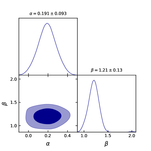
Figure 1: The $1-\sigma$ and $2-\sigma$ likelihood contours for the model parameters using $H(z)$+Pantheon+BAO datasets.

Additionally, we observed our derived model has nice fit to the aforementioned Hubble and Pantheon datasets. The error bars for the considered datasets and the $\Lambda$CDM model (with $\Omega_{\Lambda 0}=0.7$ and $\Omega_{m0}=0.3$) are also plotted along with our model for comparison. This is displayed in Fig. 2 and 3 respectively,

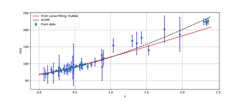
Figure 2: The figure shows the error bar plot of the considered $57$ points of Hubble datasets together with the fitting of Hubble function $H(z)$ vs. redshift $z$ for our obtained model (red line) compared with that of standard $\Lambda$CDM model (black dashed line).

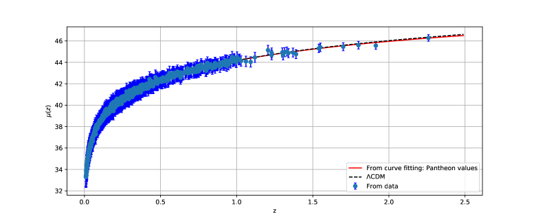
Figure 3: The figure shows the error bar plot of the considered $1048$ points of the Pantheon compilation SNe Ia datasets together with the fitting of function $\mu(z)$ vs. redshift $z$ for our obtained model (red line) compared with that of standard $\Lambda$CDM model (black dashed line).

III.2 Evolution of the $q(z)$ and phase transition

The evolution of the deceleration parameter corresponding to the constrained values of the model parameters is shown in Fig. 4. It is clear from this figure that the cosmological model contains a transition from the phase of deceleration to acceleration. The transition redshift corresponding to the values of the model parameters constrained by the combined Hubble, Pantheon and BAO datasets is $z_{t}=0.6857$. Moreover, the present value of the deceleration parameter is $q_{0}=-0.3092$. Now, we are now fully equipped with all theoretical formulas as well as numerical values of the model parameters and can discuss the physical dynamics of the model. So, the next section is dedicated to the physical dynamics of the other important cosmological parameters.

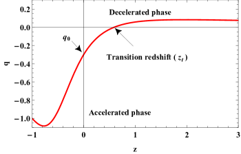
Figure 4: The graphical behavior of the deceleration parameter with the constraint values from $H(z)$+Pantheon+BAO datasets.

III.3 Statefinder analysis

As mentioned above, the deceleration parameter plays a key role in knowing the nature of the expansion of the Universe. But as more and more models are presented for DE, the deceleration parameter no longer tells us enough about the nature of the cosmological model, because DE models have the same current value of this parameter. For this reason, it has become necessary to propose new parameters to distinguish between DE models. Sahni et al. proposed a new geometrical diagnostic parameters which are dimensionless and known as statefinder parameters $\left(r,s\right)$ [42, 76]. The statefinder parameters are defined as

$$r=\frac{\overset{...}{a}}{aH^{3}},$$ (37)

$$s=\frac{\left(r-1\right)}{3\left(q-\frac{1}{2}\right)}.$$ (38)

The parameter $r$ can be rewritten as

$$r=2q^{2}+q-\frac{\overset{.}{q}}{H}.$$ (39)

For different values of the statefinder pair $\left(r,s\right)$, the various DE models known in the literature can be represented as follows

• $\Lambda$CDM model corresponds to ($r=1,s=0$),

• Chaplygin Gas (CG) model corresponds to ($r>1,s<0$),

• Quintessence model corresponds to ($r<1,s>0$),

For our cosmological model, the statefinder pair can be obtained as

$$r\left(z\right)=\frac{1-\alpha}{\beta z^{2}+z(\alpha+\beta)+1},$$ (40)

$$s\left(z\right)=\frac{2(z+1)(\alpha+\beta z)}{3\beta\left(z^{2}-1\right)+\alpha(6z-3)+9}.$$ (41)

Fig. 5 represents the $r-s$ plane by considering parameters constrained by the combined Hubble, Pantheon and BAO datasets. This plot shows that our model initially approaches the quintessence model ($r<1,s>0$). In the later epoch, it reaches the CG model ($r>1,s<0$) and finally it reaches to the fixed point of $\Lambda$CDM model ($r=1,s=0$) of the Universe.

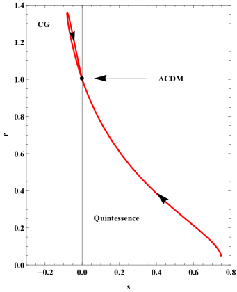
Figure 5: The graphical behavior of the statefinder parameters with the constraint values from $H(z)$+Pantheon+BAO datasets.

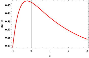
Figure 6: The graphical behavior of the Om diagnostic parameter with the constraint values from $H(z)$+Pantheon+BAO datasets.

III.4 Om diagnostics

The Om diagnostic is another very useful tool to classify the different cosmological models of DE created from the Hubble parameter [77]. It is the simplest diagnostic because it is a function of the Hubble parameter i.e. it uses only the first-order derivative of the scale factor of the Universe. In a spatially flat Universe, the Om diagnostic is defined as

$$Om\left(z\right)=\frac{E^{2}\left(z\right)-1}{\left(1+z\right)^{3}-1},$$ (42)

where $E\left(z\right)=\frac{H\left(z\right)}{H_{0}}$ and $H_{0}$ is the current Hubble constant. This tool allows us to know the dynamical nature of DE models from the slope of $Om(z)$, for a negative slope, the model behaves as quintessence while a positive slope represents a phantom behavior of the model. Lastly, the constant behavior of $Om(z)$ refers to the $\Lambda$CDM model. The Om diagnostic parameter for our model is

$$Om\left(z\right)=\frac{\alpha+\beta+\beta z}{z^{2}+3z+3}.$$ (43)

From Fig. 6, it is clear that the Om diagnostic parameter corresponding to the values of the model parameters constrained by the combined Hubble, Pantheon and BAO datasets has a negative slope at first, which indicates the quintessence type behavior, while in the future it becomes a positive slope which indicates the phantom scenario.

IV Cosmological $f\left(Q\right)$ model

In this section, we are going to discuss a cosmological models in $f(Q)$ gravity using a new parametrization of the Hubble parameter proposed in the previous section with the values of the model parameters constrained by the combined Hubble, Pantheon and BAO datasets. At this stage, the equation of state (EoS) parameter is used to classify the different phases in the expansion of the Universe i.e. from the decelerating phase to the accelerating phase and is defined as $\omega=\frac{p}{\rho}$, where $p$ is the isotropic pressure and $\rho$ is the energy density of the Universe. The simplest candidate for DE in GR is the cosmological constant $\Lambda$, for which $\omega_{\Lambda}=-1$. The value $\omega<-\frac{1}{3}$ is required for a cosmic acceleration. For other dynamical models of DE such as quintessence, $-1<\omega<-\frac{1}{3}$ and phantom regime, $\omega<-1$.

For our proposed parametrization of Hubble parameter, we assume a power-law functional form of non-metricity i.e. [25],

$$f\left(Q\right)=Q+mQ^{n},$$ (44)

where $m$ and $n$ are the free model parameters. For this specific choice of the function, by using Eqs. (24) and (25), the energy density of the Universe and the isotropic pressure can be obtained in the form

$$\rho=\frac{1}{2}\left(m\left(-6^{n}\right)(2n-1)\left(H^{2}\right)^{n}-6H^{2}\right),$$ (45)

and

$$p=\frac{2\overset{.}{H}\left(m6^{n}n(2n-1)\left(H^{2}\right)^{n}+6H^{2}\right)+3H^{2}\left(m6^{n}(2n-1)\left(H^{2}\right)^{n}+6H^{2}\right)}{6H^{2}}.$$ (46)

From Fig. 7, we can observe that the energy density of the Universe is an increasing function of redshift $z$ (or a decreasing function of cosmic time $t$) and remains positive as the Universe expands for all the three values of $n$. It begins with a positive value and gradually decreases to zero, as expected. Also, Fig. 8 shows that the isotropic pressure is an increasing function of redshift for all the three values of $n$, which starts with positive values at early times, i.e. at large $z$, and in the late and present time, the pressure becomes negative with small values close to zero. According to the observations, the negative pressure is caused by exotic matter such as dark energy in the context of accelerated expansion of the Universe. Fig. 9 depicts the behavior of the EoS parameter vs redshift using the power-law functional form of non-metricity for various values of $n$. It is clear that the model begins from a matter-dominated era ($\omega=0$) in early time, traverses the quintessence model ($-1<\omega<-\frac{1}{3}$) in the present, and then approaches the $\Lambda$CDM region ($\omega=-1$) at $z=-1$. For $n=1.5$, the EoS parameter exhibits quintessence-like behavior at the current epoch, thus both $q$ and $\omega$ give the same behaviour. Further, the present value of the EoS parameter corresponding to the combined Hubble, Pantheon, and BAO datasets and for different values of $n$ supports an accelerating phase in this scenario. Finally, it is possible to see that the behavior of the EoS parameter in our model corresponds to the models presented in the literature [29, 30, 31].

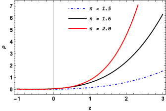
Figure 7: The graphical behavior of the energy density with the constraint values from $H(z)$+Pantheon+BAO datasets and different values for $n$.

Figure 8: The graphical behavior of the isotropic pressure with the constraint values from $H(z)$+Pantheon+BAO datasets and different values for $n$.

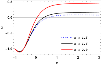
Figure 9: The graphical behavior of the EoS parameter with the constraint values from $H(z)$+Pantheon+BAO datasets and different values for $n$.

V Conclusions

In this paper, we investigated the accelerated expansion of the Universe in the framework of $f\left(Q\right)$ gravity theory in which the non-metricity scalar $Q$ describes the gravitational interaction. To find the exact solutions to the field equations in the FLRW Universe, we proposed a new parametrization of the Hubble parameter, specifically, $H\left(z\right)=H_{0}\left[\left(1-\alpha\right)+\left(1+z\right)\left(\alpha+\beta z\right)\right]^{\frac{1}{2}}$ where $\alpha$ and $\beta$ are free model parameters, $H_{0}$ represents the present value of the Hubble parameter. Further, we obtained the best fit values of the model parameters by using the combined Hubble $H\left(z\right)$, Pantheon and BAO datasets as $\alpha=0.191_{-0.093}^{+0.093}$, $\beta=1.21_{-0.13}^{+0.13}$. In addition, we have investigated the behavior of deceleration parameter, statefinder analysis and Om diagnostic parameter for the constrained values of model parameters. The evolution of the deceleration parameter in Fig. 4 indicates that our cosmological contains a transition from decelerated to accelerated phase. The transition redshift corresponding to the values of the model parameters constrained by the combined Hubble, Pantheon and BAO datasets is $z_{t}=0.6857$. Moreover, the present value of the deceleration parameter is $q_{0}=-0.3092$. Further, Fig 5 represents the $r-s$ evolution trajectories of the model which initially approaches the quintessence model. In the later epoch, it reaches the CG model and finally it reaches to the fixed point of $\Lambda$CDM model of the Universe. The Om diagnostic parameter has a negative slope at first, which indicates the quintessence type behavior, while in the future it becomes a positive slope which indicates the phantom scenario. Next, to discuss the behavior of other cosmological parameters, we considered a $f(Q)$ model of the non-metricity scalar, specifically, $f\left(Q\right)=Q+mQ^{n}$, where $m$ and $n$ are free parameters. From Fig. 7 we observed that the energy density is positive values and increasing function of redshift. This represents the expansion of the Universe. The variation of the isotropic pressure is presented in Fig. 8. From the figure, we observed that the isotropic pressure is negative at present and later times. From EoS parameter (see Fig. 9) we observed that $f(Q)$ model exhibits quintessence-like behavior at the current epoch. Finally, we conclude that the model supports the current accelerating Universe.

Data availability There are no new data associated with this article.

Declaration of competing interest The authors declare that they have no known competing financial interests or personal relationships that could have appeared to influence the work reported in this paper.

- [1] A.G. Riess et al., Astron. J. 116, 1009 (1998).
- [2] S. Perlmutter et al., Astrophys. J. 517, 565 (1999).
- [3] T. Koivisto, D.F. Mota, Phys. Rev. D 73, 083502 (2006).
- [4] S.F. Daniel, Phys. Rev. D 77, 103513 (2008).
- [5] C.L. Bennett et al., Astrophys. J. Suppl. 148, 119-134 (2003).
- [6] D.N. Spergel et al., [WMAP Collaboration], Astrophys. J. Suppl. 148, 175 (2003).
- [7] G. Hinshaw et al., Astrophys. J. Suppl. 208, 19 (2013).
- [8] R.R. Caldwell, M. Doran, Phys. Rev. D 69, 103517 (2004).
- [9] Z.Y. Huang et al., JCAP 0605, 013 (2006).
- [10] D.J. Eisenstein et al., Astrophys. J. 633, 560 (2005).
- [11] W.J. Percival at el., Mon. Not. R. Astron. Soc. 401, 2148 (2010).
- [12] S.Weinberg, Rev. Mod. Phys. 61, 1 (1989).
- [13] B. Ratra and P.J.E. Peebles, Phys. Rev. D 37, 3406 (1998).
- [14] M. Sami and A. Toporensky, Mod. Phys. Lett. A 19, 1509 (2004).
- [15] C. Armendariz-Picon et al., Phys. Rev. Lett. 85, 4438 (2000).
- [16] J. Khoury and A. Weltman, Phys. Rev. Lett. 93, 171104 (2004).
- [17] T. Padmanabhan, Phys. Rev. D 66, 021301 (2002).
- [18] M. C. Bento et al., Phys. Rev. D 66, 043507 (2002).
- [19] R. Zarrouki and M. Bennai, Phys. Rev. D 82, 123506 (2010).
- [20] S. Capozziello et al., Phys. Rev. D 76, 104019 (2007).
- [21] M. Koussour and M. Bennai, Class. Quantum Gravity 39, 105001 (2022).
- [22] J. B. Jimenez et al., Phys. Rev. D 98, 044048 (2018).
- [23] J. B. Jimenez et al., Phys. Rev. D 101, 103507 (2020).
- [24] Y. Xu et al., Eur. Phys. J. C 79, 8 (2019).
- [25] S. Mandal et al., Phys. Rev. D 102, 024057 (2020).
- [26] S. Mandal et al., Phys. Rev. D 102, 124029 (2020).
- [27] T. Harko et al., Phys. Rev. D 98, 084043 (2018).
- [28] N. Dimakis et al., Class. Quantum Grav. 38, 225003 (2021).
- [29] M. Koussour et al., J. High Energy Astrophys, 35, 43-51 (2022).
- [30] M. Koussour et al., Phys. Dark Universe 36, 101051 (2022).
- [31] S. Mandal et al., Universe 8, 4 (2022).
- [32] R. Lazkoz et al., Phys. Rev. D 100, 104027 (2019).
- [33] G. S. Sharov et al., Mon. Not. R. Astron. Soc. 466, 3497 (2017).
- [34] D.M. Scolnic et al., Astrophys. J. 859, 101 (2018).
- [35] C. Blake et al., Mon. Not. Roy. Astron. Soc. 418, 1707 (2011).
- [36] D. F. Mackey et al., Publ. Astron. Soc. Pac. 125, 306 (2013).
- [37] J. B. Jimenez, L. Heisenberg, and T. S. Koivisto, J. Cosmol. Astropart. Phys. 2018, 08 (2018).
- [38] L. Heisenberg, Phys. Rep. 796, 1-113 (2019).
- [39] J. B. Jimenez, L. Heisenberg, and T. S. Koivisto, Universe 5, 7 (2019).
- [40] L. Heisenberg, M. Hohmann, and S. Kuhn, arXiv preprint arXiv:2212.14324 (2022).
- [41] A. Shafieloo et al., Phys. Rev. D 87, 2 (2013).
- [42] V. Sahni, T. D. Saini, A. A. Starobinsky, U. Alam, JETP Lett. 77, 201 (2003).
- [43] C. Escamilla-Rivera and A. Najera, J. Cosmol. Astropart. Phys. 2022, 03 (2022).
- [44] N. Banerjee, S. Das, Gen. Relativ. Gravit. 37, 1695 (2005).
- [45] J. V. Cunha and J. A. S. Lima, Mon. Not. Roy. Astr. Soc. 390, 210 (2008).
- [46] S. K. J. Pacif et al., Int. J. Geom. Meth. Mod. Phys. 14, 7 (2017).
- [47] S. K. J. S. K. J. Pacif, Eur. Phys. J. Plus135, 10 (2020).
- [48] D. Stern et al., J. Cosmol. Astropart. Phys., 02 008 (2010).
- [49] J. Simon, L. Verde, R. Jimenez, Phys. Rev. D 71 123001 (2005).
- [50] M. Moresco et al., J. Cosmol. Astropart. Phys., 08 006 (2012).
- [51] C. Zhang et al., Research in Astron. and Astrop., 14 1221 (2014).
- [52] M. Moresco et al., J. Cosmol. Astropart. Phys., 05 014 (2016).
- [53] A. L. Ratsimbazafy et al., Mon. Not. Roy. Astron. Soc.,467 3239 (2017).
- [54] M. Moresco, Mon. Not. Roy. Astron. Soc. Lett., 450 L16 (2015).
- [55] E. Gaztaaga et al., Mon. Not. Roy. Astron. Soc., 399 1663 (2009).
- [56] A. Oka et al., Mon. Not. Roy. Astron. Soc., 439 2515 (2014).
- [57] Y. Wang et al., Mon. Not. Roy. Astron. Soc., 469 3762 (2017).
- [58] C. H. Chuang, Y. Wang, Mon. Not. Roy. Astron. Soc., 435 255 (2013).
- [59] S. Alam et al., Mon. Not. Roy. Astron. Soc., 470 2617 (2017).
- [60] C. Blake et al., Mon. Not. Roy. Astron. Soc., 425 405 (2012).
- [61] C. H. Chuang et al., Mon. Not. Roy. Astron. Soc., 433 3559 (2013).
- [62] L. Anderson et al., Mon. Not. Roy. Astron. Soc., 441 24 (2014).
- [63] N. G. Busca et al., Astron. Astrophys., 552 A96 (2013).
- [64] J. E. Bautista et al., Astron. Astrophys., 603 A12 (2017).
- [65] T. Delubac et al., Astron. Astrophys., 574 A59 (2015).
- [66] A. Font-Ribera et al., J. Cosmol. Astropart. Phys., 05 027 (2014).
- [67] D. M. Scolnic et al., Astrophys. J., 859 101 (2018).
- [68] C. Blake et al., Mon. Not. Roy. Astron. Soc., 418 1707 (2011).
- [69] F. Beutler et al., Mon. Not. Roy. Astron. Soc., 416, 3017 (2011).
- [70] N. Jarosik et al., Astrophys. J. Suppl., 192 14 (2011).
- [71] R. Giostri et al., J. Cosm. Astropart. Phys., 03 027 (2012).
- [72] M. Chevallier, D. Polarski, Int. J. Mod. Phys. D 10, 213 (2001).
- [73] S. Del Campo et al., Phys. Rev. D 86, 083509 (2012).
- [74] S. Joan , Phys. Rev. D 71 (2005) 255-262. [arXiv:1209.0210]
- [75] J. E. Bautista et al., Astron. Astrophys. 603 (2017) A12.
- [76] U. Alam et al., Mon. Not. R. Astron. Soc. 344, 1057 (2003).
- [77] V. Sahni, A. Shafieloo, and A. A. Starobinsky, Phys. Rev. D 78, 103502 (2008).
- [78] E. M. Barboza Jr and J. S. Alcaniz, Phys. Lett. B 666, 5 (2008).
- [79] H. Wei et al., J. Cosmol. Astropart. Phys. 2014, 01 (2014).