Equilibrium and non-equilibrium dynamics of a hole in a bilayer antiferromagnet

Abstract

The dynamics of charge carriers in lattices of quantum spins is a long standing and fundamental problem. Recently, a new generation of quantum simulation experiments based on atoms in optical lattices has emerged that gives unprecedented insights into the detailed spatial and temporal dynamics of this problem, which compliments earlier results from condensed matter experiments. Focusing on observables accessible in these new experiments, we explore here the equilibrium as well as non-equilibrium dynamics of a mobile hole in two coupled antiferromagnetic spin lattices. Using a self-consistent Born approximation, we calculate the spectral properties of the hole in the bilayer and extract the energy bands of the quasiparticles, corresponding to magnetic polarons that are either symmetric or anti-symmetric under layer exchange. These two kinds of polarons are degenerate at certain momenta due to the antiferromagnetic symmetry, and we, furthermore, examine how the momentum of the ground state polaron depends on the interlayer coupling strength. The long time dynamics of a hole initially created in one layer is shown to be characterised by oscillations between the two layers with a frequency given by the energy difference between the symmetric and the anti-symmetric polaron. We finally demonstrate that the expansion velocity of a hole initially created at a given lattice site is governed by the ballistic motion of polarons. It moreover depends non-monotonically on the interlayer coupling, eventually increasing as a quantum phase transition to a disordered state is approached.

I Introduction

The motion of charge carriers in doped antiferromagnetic (AF) layers is a key problem in quantum many-body physics that has been studied intensely since the discovery of high temperature superconductivity. In the cuprates Keimer et al. (2015) as well as in other strongly correlated two-dimensional (2D) materials such as the pnictides Wen and Li (2011), organic layers Wosnitza (2012), and twisted bilayer graphene Cao et al. (2018), pairing exists close to the magnetically ordered phase. The competition between hole motion and AF order, therefore, provides important clues for the physics of these unconventional superconductors Dagotto (1994); Lee et al. (2006). For small hole doping, the hole dynamics is described by the ubiquitous $t$-$J$ model, which is able to quantitatively explain photoemission experiments from insulating cuprates when treated within the so-called self-consistent Born approximation (SCBA) Damascelli et al. (2003). The dressing of the hole by magnetic frustration in its vicinity leads to the formation of quasiparticles coined magnetic polarons Schmitt-Rink et al. (1988); Shraiman and Siggia (1988); Kane et al. (1989); Martinez and Horsch (1991); Liu and Manousakis (1991), which play a key role for understanding the properties of doped AF layers. It is well-known that the SCBA yields an accurate description of the equilibrium properties of the magnetic polaron Martinez and Horsch (1991); Liu and Manousakis (1991); Marsiglio et al. (1991); Chernyshev and Leung (1999); Diamantis and Manousakis (2021), and recently this was shown to hold for the non-equilibrium properties as well Nielsen et al. (2022). Since the unit cell of some cuprates can have two or more CuO₂ planes, magnetic polarons have also been studied in multi-layer systems Nazarenko and Dagotto (1996); Yin and Gong (1997, 1998). Such systems are also interesting because they exhibit a quantum phase transition between long range AF order and a disordered state of spin singlets across the layers Hida (1992); Sandvik and Scalapino (1994); Scalettar et al. (1994); Millis and Monien (1994); Sandvik et al. (1995); Chubukov and Morr (1995).

Mobile charge carriers in two-dimensional (2D) quantum AF magnets has recently received renewed interest due to a novel generation of experiments using ultracold atoms in optical lattices Carlström et al. (2016); Kanász-Nagy et al. (2017); Grusdt et al. (2018a, b); Nielsen et al. (2021, 2022). These experiments provide an essentially perfect realization of the Fermi-Hubbard model and combined with their single site resolution imaging, they represent a powerful quantum simulator for exploring the interplay between charge carriers and magnetic order in doped AFs Chiu et al. (2019); Brown et al. (2019); Koepsell et al. (2019); Ji et al. (2021); Koepsell et al. (2021). Recently, also bilayer Gall et al. (2021) and ladder geometries Hirthe et al. (2022) have been realised with optical lattices.

Figure 1: A hole in an AF bilayer. The blue and red balls represent fermions with spin up and down respectively, and the green circle the hole. Reading from left to right, we see the hole propagating in the AF background, destroying the AF order around it. The delocalization of the hole and the AF order are, therefore, two competing dynamics of the system.

Here, we explore a single mobile hole in a bilayer system consisting of two square lattices of spins with AF order. We analyze the spectral properties of the hole as a function of the system parameters using a diagrammatic approach based on the SCBA, and we discuss the properties of the two kinds of magnetic polarons existing in the system, which are either symmetric or antisymmetric under layer exchange. Focusing on observables that are accessible in the new optical lattice experiments, we show that these polarons give rise to intriguing non-equilibrium effects of the hole such as oscillations between the two layers, and a long time expansion velocity that first decreases and then increases with the interlayer coupling as the spins approach a quantum phase transition to a disordered state.

II Model

We consider a single mobile hole in an antiferromagnetic (AF) bilayer formed by two square lattices as illustrated in Fig. 1. The dynamics of the hole is described by the $t$-$J$ model with the Hamiltonian

$$\hat{H}=\hat{H}_{t}+\hat{H}_{J}$$ (1)

where

$$\hat{H}_{t}=-t\sum_{l,\langle{\bf i},{\bf j}\rangle,\sigma}\tilde{c}^{\dagger}_{l,{\bf i},\sigma}\tilde{c}_{l,{\bf j},\sigma}-t_{\perp}\sum_{{\bf i},\sigma}\tilde{c}^{\dagger}_{1,{\bf i},\sigma}\tilde{c}_{2,{\bf j},\sigma}+\text{h.c.}$$ (2)

and

$$\hat{H}_{J}= \ J\sum_{l,\langle{\bf i},{\bf j}\rangle}\left[\hat{\mathbf{S}}_{l,{\bf i}}\cdot\hat{\mathbf{S}}_{l,{\bf j}}-\frac{1}{4}\hat{n}_{l,{\bf i}}n_{l,{\bf j}}\right]+$$

$$\ J_{\perp}\sum_{{\bf i}}\left[\hat{\mathbf{S}}_{1,{\bf i}}\cdot\hat{\mathbf{S}}_{2,{\bf i}}-\frac{1}{4}\hat{n}_{1,{\bf i}}\hat{n}_{2,{\bf i}}\right]$$ (3)

Here, $\tilde{c}^{\dagger}_{l,{\bf i},\sigma}=\hat{c}^{\dagger}_{l,{\bf i},\sigma}(1-\hat{n}_{l,{\bf i},\bar{\sigma}})$ where $\hat{c}^{\dagger}_{l,{\bf i},\sigma}$creates a fermion in layer $l=1,2$ at site $\mathbf{i}$ with spin $\sigma=\uparrow,\downarrow$. The factor $1-\hat{n}_{l,{\bf i},\bar{\sigma}}$ with $\hat{n}_{l,{\bf i},\bar{\sigma}}=\hat{c}^{\dagger}_{l,{\bf i},\bar{\sigma}}\hat{c}_{l,{\bf i},\bar{\sigma}}$ and $\bar{\sigma}$ the opposite spin of $\sigma$ ensures that no site is doubly occupied. The matrix elements for inter- and intralayer hopping are $t$ and $t_{\perp}$, and the AF coupling between neighbouring spins within the same layer and in different layers is $J>0$ and $J_{\perp}>0$ respectively. Also, the spin $1/2$ operators are given in terms of the fermions via the Schwinger representation

$$\hat{{\bf S}}_{l,\bf i}=\frac{1}{2}\sum_{\sigma,\sigma^{\prime}}\hat{c}^{\dagger}_{l,{\bf i},\sigma}\boldsymbol{\sigma}_{\sigma\sigma^{\prime}}\hat{c}_{l,{\bf i},\sigma^{\prime}},$$ (4)

with $\boldsymbol{\sigma}=(\sigma_{x},\sigma_{y},\sigma_{z})$ a vector of Pauli matrices. Taking $J=4t^{2}/U$ and $J_{\perp}=4t_{\perp}^{2}/U$, the $t$-$J$ model provides an effective low-energy description of the Fermi-Hubbard model with strong onsite repulsion $U\gg t$  Chao et al. (1977); Reischl et al. (2004), but it can also be regarded as an independent model in itself. One can for instance realize models with $J_{\perp}\neq 4t_{\perp}^{2}/U$ using atoms in optical lattices Grusdt et al. (2018a); Koepsell et al. (2020) as well as using Rydberg atoms in optical tweezers Browaeys and Lahaye (2020).

II.1 Slave-fermion representation

To describe the motion of a single hole in the bilayer, we perform a Holstein-Primakoff transformation generalized to the case where a hole is present Kane et al. (1989); Martinez and Horsch (1991); Liu and Manousakis (1991); Schmitt-Rink et al. (1988); Nielsen et al. (2021). Due to the AF order, we can for each layer define two sublattices A and B where the spins will predominantly point up in sublattice A and down in B. A site in sublattice A in layer 1 is adjacent to a site in sublattice B in layer 2 and vice versa, see Fig. 1. For sublattice A, the spin operators are expressed as $\hat{S}^{z}_{l,{\mathbf{i}}}=(1-\hat{h}^{\dagger}_{l,{\mathbf{i}}}\hat{h}_{l,{\mathbf{i}}})/2-\hat{s}^{\dagger}_{l,{\mathbf{i}}}\hat{s}_{l,{\mathbf{i}}}$ and $\hat{S}_{l,{\mathbf{i}}}^{-}=\hat{S}^{x}_{l,{\mathbf{i}}}-i\hat{S}^{y}_{l,{\mathbf{i}}}=\hat{s}^{\dagger}_{l,{\mathbf{i}}}(1-\hat{s}^{\dagger}_{l,{\mathbf{i}}}\hat{s}_{l,{\mathbf{i}}}-\hat{h}^{\dagger}_{l,{\mathbf{i}}}\hat{h}_{l,{\mathbf{i}}})^{1/2}$, and the creation operators are $\tilde{c}_{i,{\downarrow}}=\hat{h}^{\dagger}_{l,{\mathbf{i}}}\hat{s}_{l,{\mathbf{i}}}$ and $\tilde{c}_{i,{\uparrow}}=\hat{h}^{\dagger}_{l,{\mathbf{i}}}(1-\hat{s}^{\dagger}_{l,{\mathbf{i}}}\hat{s}_{l,{\mathbf{i}}}-\hat{h}^{\dagger}_{l,{\mathbf{i}}}\hat{h}_{l,{\mathbf{i}}})^{1/2}$. Here, $\hat{h}^{\dagger}_{l,{\mathbf{i}}}$ is a fermionic creation operator of a hole and $\hat{s}^{\dagger}_{l,{\mathbf{i}}}$ is a bosonic creation operator of a spin-fluctuation. The square root $(1-\hat{s}^{\dagger}_{l,{\mathbf{i}}}\hat{s}_{l,{\mathbf{i}}}-\hat{h}^{\dagger}_{l,{\mathbf{i}}}\hat{h}_{l,{\mathbf{i}}})^{1/2}$ give a combined hardcore constraint for both spin excitations and holes. Operators on sublattice B take similar form Nielsen et al. (2021).

Applying this so-called slave-fermion representation to the spin part of the Hamiltonian given by Eq. (3) and keeping only linear terms yields after diagonalization

$$\hat{H}_{J}=E_{0}+\sum_{{\bf k},\mu=\pm}\omega_{\mu,{\bf k}}\hat{b}^{\dagger}_{\mu,{\bf k}}\hat{b}_{\mu,{\bf k}}.$$ (5)

Here, $E_{0}=-{J_{\perp}}(2N-1)/{2}-{Jz}(2N-1)/{2}+\sum_{\textbf{k},\mu=\pm}\omega_{\mathbf{k},\mu}/2$ is the ground state energy with $N$ the number of lattice sites in each plane, and

$$\omega_{\pm,{\bf k}}= \ \frac{1}{2}\sqrt{\left(Jz+J_{\perp}\right)^{2}-(Jz\gamma_{{\bf k}}\pm J_{\perp})^{2}}$$ (6)

is the spin wave spectrum, with the structure factor $\gamma_{{\bf k}}=\sum_{{\boldsymbol{\delta}}}{\rm e}^{i{\bf k}\cdot{\boldsymbol{\delta}}}/z=(\cos{k_{x}}+\cos{k_{y}})/2$. Here, $z=4$ is the coordination number and ${\boldsymbol{\delta}}$ are the nearest neighbor sites, while the crystal momentum ${{\bf k}}$ is in the first Brillouin zone (BZ) of the square lattice Nazarenko and Dagotto (1996); Yin and Gong (1997, 1998). We take the lattice constant to be unity throughout. The bilayer has two spin wave branches $\mu=\pm$, which are connected to the spin fluctuation operators by a unitary and a Bogoliubov transformation

$$\begin{bmatrix}\hat{s}_{1,{\bf k}}\\ \hat{s}^{\dagger}_{1,-{\bf k}}\\ \hat{s}_{2,{\bf k}}\\ \hat{s}^{\dagger}_{2,-{\bf k}}\end{bmatrix}=\frac{1}{\sqrt{2}}\begin{bmatrix}\mathds{1}&-\mathds{1}\\ \mathds{1}&\mathds{1}\end{bmatrix}\begin{bmatrix}U_{+,{\bf k}}&0\\ 0&U_{-,{\bf k}}\end{bmatrix}\begin{bmatrix}\hat{b}_{+,{\bf k}}\\ \hat{b}^{\dagger}_{+,-{\bf k}}\\ \hat{b}_{-,{\bf k}}\\ \hat{b}^{\dagger}_{-,-{\bf k}}\end{bmatrix}.$$ (7)

Here, $\mathds{1}=\begin{bmatrix}1&0\\ 0&1\end{bmatrix}$ and $U_{\pm,{\bf k}}=\begin{bmatrix}u_{\pm,{\bf k}}&-v_{\pm,{\bf k}}\\ -v_{\pm,{\bf k}}&u_{\pm,{\bf k}}\end{bmatrix}$ with the coherence factors

$$u_{\pm,{\bf k}} =\sqrt{\frac{1}{2}\left(\frac{zJ+J_{\perp}}{2\omega_{\pm,{\bf k}}}+1\right)}$$

$$v_{\pm,{\bf k}} ={\rm sgn}\left[zJ\gamma_{\bf k}\pm J_{\perp}\right]\sqrt{\frac{1}{2}\left(\frac{zJ+J_{\perp}}{2\omega_{\pm,{\bf k}}}-1\right)}.$$ (8)

Operators in momentum space are connected to operators in real space via the usual discrete Fourier transform $\hat{s}_{l,{{\bf k}}}=\sum_{\mathbf{i}}\hat{s}_{l,{\mathbf{i}}}\exp(-i{{\bf k}}\cdot{\mathbf{i}})/\sqrt{N}$. The full details of the diagonalization of $\hat{H}_{J}$ can be found in Appendix A. Figure 2 shows the spin wave dispersion for the two branches taking $J_{\perp}/J=0.25$. At low momenta, the $\mu=+$ branch corresponds to spin waves in the two planes being in-phase giving a Goldstone mode for ${\bf k}\rightarrow 0$. This is reversed close to ${\bf p}=(\pi,\pi)$ where the $\mu=-$ mode corresponds to the spin waves in the two planes being in-phase. More generally, we have $\omega_{+,{\bf k}+\mathbf{Q}}=\omega_{-,{\bf k}}$ where $\mathbf{Q}=(\pi,\pi)$ is the AF ordering vector, so that the full spin wave spectrum displays the expected symmetry from the AF order.

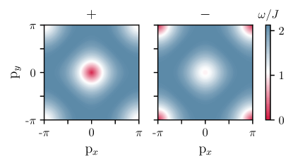
Figure 2: Spin wave dispersion. The left and right panel show the spin wave dispersion given by Eq. (6) for the $\mu=+$ and $\mu=-$ branches respectively with $J_{\perp}/J=0.25$.

Likewise, using the slave fermion representation for $\hat{H}_{t}$ yields

$$\hat{H}_{t}= \sum_{{\bf k},{\bf p},l}\hat{h}_{l,{\bf p}+{\bf k}}^{\dagger}\hat{h}_{l,{\bf p}}[g_{+}({\bf p},{\bf k})\hat{b}^{\dagger}_{+,-{\bf k}}+(-1)^{l}g_{-}({\bf p},{\bf k})\hat{b}^{\dagger}_{-,-{\bf k}}]$$

$$+\sum_{{\bf k},{\bf p}}\hat{h}_{2,{\bf p}+{\bf k}}^{\dagger}\hat{h}_{1,{\bf p}}[f_{+}({\bf k})(\hat{b}_{+,{\bf k}}+\hat{b}^{\dagger}_{+,-{\bf k}})$$

$$+f_{-}({\bf k})(\hat{b}_{-,{\bf k}}-\hat{b}^{\dagger}_{-,-{\bf k}})]+\text{h.c.}.$$ (9)

Here

$$g_{\pm}({\bf p},{\bf k})=\frac{zt}{\sqrt{2N}}\left[u_{\pm,{\bf k}}\gamma_{{\bf p}+{\bf k}}-v_{\pm,{\bf k}}\gamma_{\bf p}\right]$$ (10)

is the vertex describing the scattering between a hole and a spin wave where the hole remains in a given layer, and

$$f_{\pm}({\bf k})=\frac{t_{\perp}}{\sqrt{2N}}\left[u_{\pm,{\bf k}}\mp v_{\pm,{\bf k}}\right]$$ (11)

is the scattering vertex when the hole jumps from one layer to the other. Equation (9) quantitatively describes how the motion of the hole distorts the AF order by the emission of spin waves. The inter-layer vertices $f_{\pm}({\bf k})$ vanish when $t_{\perp}=0$ and the Hamiltonian then simplifies to two copies of a single layer as expected. The interaction vertices satisfy the symmetries

$$g_{\pm}({\bf p},{\bf k}+{\bf Q}) =-g_{\mp}({\bf p},{\bf k}),\;g_{\pm}({\bf p}+{\bf Q},{\bf k})=-g_{\pm}({\bf p},{\bf k})$$

$$f_{\pm}({\bf k}+{\bf Q}) =f_{\mp}({\bf k})$$ (12)

due to the underlying AF order.

III Symmetric and anti-symmetric polarons

The competition between the hole motion and the magnetic order leads to the formation of quasiparticles where the hole is surrounded by a cloud of reduced AF order Schmitt-Rink et al. (1988); Shraiman and Siggia (1988); Kane et al. (1989); Martinez and Horsch (1991); Liu and Manousakis (1991). These quasiparticles, named magnetic polarons, play a central role for the equilibrium as well as non-equilibrium properties of the system. The bilayer symmetry $\hat{c}_{1,{\bf i}}\leftrightarrow\hat{c}_{2,{\bf i}}$ of Eq. (1), means that the polaron states can be divided into those symmetric and antisymmetric under layer exchange. The wave function for the polarons can be expressed as a series of terms with an increasing number of spin waves on top of the AF ground state, i.e.

$$|\Psi_{\mathbf{p}}^{\pm}\rangle= \ \sqrt{\frac{Z_{\mathbf{p}}^{\pm}}{2}}(\hat{h}^{\dagger}_{1,\mathbf{p}}\pm\hat{h}^{\dagger}_{2,\mathbf{p}})|\text{AF}\rangle+$$

$$\ \sum_{{\mathbf{k}},\mu,l}\phi^{\pm}_{l,\mu}({\mathbf{p}},\mathbf{k})\hat{h}^{\dagger}_{l,{\mathbf{p}}+{\mathbf{k}}}\hat{b}^{\dagger}_{\mu,-{\mathbf{k}}}|\text{AF}\rangle\ldots.$$ (13)

Here, $|\text{AF}\rangle$ is the AF ground state defined by $\hat{b}_{\mu,{\mathbf{k}}}|\text{AF}\rangle=0$, $Z_{\mathbf{p}}^{\pm}$ is the quasiparticle residue, and $\phi^{\pm}_{l,\mu}({\mathbf{p}},\mathbf{k})$ is the coefficient for the term involving a hole with momentum ${\mathbf{p}}+\mathbf{k}$ in layer $l$ and a spin wave in branch $\mu$ with momentum $-\mathbf{k}$. For a single layer, one has developed diagrammatic rules for constructing the wave function corresponding to the SCBA, which was used to calculate terms including up to three spin waves Reiter (1994); Ramšak and Horsch (1998); Ramsak and Horsch (1993). Recently, this has been extended to infinite order in the number of spin waves by deriving a set of Dyson like equations Nielsen et al. (2021).

IV Self-consistent Born approximation

We use the self-consistent Born approximation (SCBA) Schmitt-Rink et al. (1988); Kane et al. (1989) generalized to the case of a bilayer to analyze the properties of the hole Nazarenko and Dagotto (1996); Yin and Gong (1997, 1998). For a single layer, the SCBA is known to yield quantitatively accurate results for the equilibrium properties of the hole Martinez and Horsch (1991); Liu and Manousakis (1991); Marsiglio et al. (1991); Liu and Manousakis (1992); Chernyshev and Leung (1999); Diamantis and Manousakis (2021), and recently this has been shown to hold for the non-equilibrium dynamics as well Nielsen et al. (2022).

The layer degree of freedom gives rise to a $2\times 2$ matrix structure for the equilibrium Green’s function for the hole, which we define as

$$G_{lm}({\bf p},\tau)=-\braket{T_{\tau}\left[\hat{h}_{l,{\bf p}}(\tau)\hat{h}^{\dagger}_{m,{\bf p}}(0)\right]},$$ (14)

where $T$ is time ordering in imaginary time $\tau$. We have $G_{11}({\bf p},\tau)=G_{22}({\bf p},\tau)\equiv G_{\rm d}({\bf p},\tau)$ and $G_{12}({\bf p},\tau)=G_{21}({\bf p},\tau)\equiv G_{\rm o}({\bf p},\tau)$ due to the layer symmetry. The Dyson equation reads in frequency space

$$G(p)=\mathds{1}_{2}G_{0}(p)+G_{0}(p)\Sigma(p)G(p),$$ (15)

where $p=({\bf p},i\omega_{p})$ with $i\omega_{p}$ a fermionic Matsubara frequency. The non-interacting hole Green’s function is $G_{0}(p)=1/i\omega_{p}$ independent of the crystal momentum since there is no kinetic energy term for the hole in $\hat{H}_{t}$ given Eq. (9). The self-energy matrix is

$$\Sigma(p)=\begin{bmatrix}\Sigma_{\rm d}(p)&\Sigma_{\rm o}(p)\\ \Sigma_{\rm o}(p)&\Sigma_{\rm d}(p)\end{bmatrix}.$$ (16)

From Eq. (15) we find

$$G_{\rm d}(p)=\frac{i\omega_{p}-\Sigma_{\rm d}(p)}{[i\omega_{p}-\Sigma_{\rm d}(p)]^{2}-\Sigma_{\rm o}(p)^{2}}$$

$$G_{\rm o}(p)=\frac{\Sigma_{\rm o}(p)}{[i\omega_{p}-\Sigma_{\rm d}(p)]^{2}-\Sigma_{\rm o}(p)^{2}}.$$ (17)

To proceed with the calculation of these self-energies, we now invoke our essential approximation scheme, i.e. the self-consistent Born approximation (SCBA). Diagrammatically, the SCBA corresponds to the inclusion of all rainbow diagrams, as shown in Fig. 3. By using the symmetries in Eq. (12) and the expressions for the Green’s functions Eq. (17), the self-energies can for zero temperature be written in a compact matrix form as

$$\Sigma({\bf p},\omega)=2\sum_{{\bf k}}V^{2}_{+}({\bf p},{\bf k})G({\bf p}+{\bf k},\omega-\omega_{+,{\bf k}}),$$ (18)

where

$$V_{+}({\bf p},{\bf k})=\begin{bmatrix}g_{+}({\bf p},{\bf k})&f_{+}({\bf k})\\ f_{+}({\bf k})&g_{+}({\bf p},{\bf k})\end{bmatrix},$$ (19)

and the factor of $2$ reflects that the two spin wave branches contribute equally to the self-energies. Here, we have performed the usual analytical continuation $i\omega_{p}\to\omega+i0_{+}$ to get the retarded Green’s functions. The structure of Eq. (18) for the self-energy is the same as for a single layer Kane et al. (1989); Martinez and Horsch (1991) with the vertex functions replaced by matrices. Equations (17)-(18) constitute our self-consistent equations, which we solve iteratively starting from $\Sigma=0$.

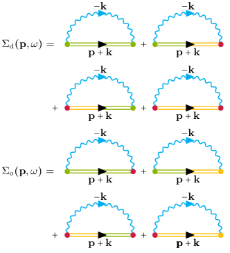
Figure 3: SCBA diagrams. Feynman diagrams included in the calculation of $\Sigma_{\text{d}}$ and $\Sigma_{\text{o}}$. The green color is associated with layer $l=1$ and yellow with $l=2$. Green and yellow vertices are associated with the intra-layer interactions, i.e. the hole continuous to propagate in the same layer after the interaction. The red vertex is associated with interactions where the hole jumps from one layer to the other. The propagators containing two colors represent $G_{\text{o}}$.

V Equilibrium properties

We now analyze the equilibrium properties of mobile holes in the bilayer. While this problem has been explored by several authors, we focus on aspects important for the new generation of optical lattice experiments. The analysis in this section also lays the foundation for the understanding non-equilibrium dynamics described in Sec. VI.

We calculate the hole spectral functions ${A}_{\rm d/\rm o}({\bf p},\omega)=-2\text{Im}[G_{\rm d/\rm o}({\bf p},\omega)]$ by solving (17)-(18) numerically for a pair of $28\times 28$ lattices. The diagonal spectral function ${A}_{\rm d}({\bf p},\omega)$ is associated with the motion of a hole within a given layer whereas the off-diagonal spectral function ${A}_{\rm o}({\bf p},\omega)$ is associated with the hole starting in one layer and ending up in the other. Using the interlayer hopping matrix element $t$ as an energy unit, we have three free parameters: $J/t$, $J_{\perp}/t$, and $t_{\perp}/t$. To be specific and to reduce parameter space, we vary $J/t$ and $t_{\perp}/t$ keeping $J_{\perp}=4t_{\perp}^{2}/U=(t_{\perp}/t)^{2}J$ inspired by the connection to the Hubbard model.

Figure 4(a) shows the hole spectral functions for the momentum ${\bf p}={\bf Q}/2=(\pi/2,\pi/2)$, $J/t=0.3$, and two different values of $t_{\perp}/t$.

Figure 4: Hole spectral functions. Panel $\mathrm{(a)}$ shows the spectral functions for ${\bf p}=(\pi/2,\pi/2)$ with $J/t=0.3$ and $t_{\perp}/t=0$ (dashed) as well as $t_{\perp}/t=1$ (solid). The quasiparticle peaks at $\omega/t\simeq-2.3$ and $\omega/t\simeq-2.5$ for $t_{\perp}/t=0$ and $t_{\perp}/t=1$ respectively give the energy of the magnetic polaron. As expected, the off-diagonal spectral function vanishes for $t_{\perp}=0$ and it also vanishes for $t_{\perp}/t=1$ due to the AF order. Panel $\mathrm{(b)}$ shows the spectral functions for ${\bf p}=(0,0)$ where both the diagonal and off-diagonal parts are non-zero and have the same poles.

Consider first the case of a vanishing interlayer hopping $t_{\perp}/t=0$, which corresponds to the two layers being decoupled so that ${A}_{\rm o}=0$. The diagonal spectral function ${A}_{\rm d}$ exhibits a clear quasiparticle peak at $\omega/t\simeq-2.3$ in agreement with previous results for a single layer magnetic polaron Nielsen et al. (2021). This polaron is one of four degenerate ground states with momenta ${\bf p}=(\pm\pi/2,\pm\pi/2)$ for each layer. The broad peaks at higher energies in Fig. 4(a) can be interpreted as damped string excitations of the magnetic polaron Nielsen et al. (2022).

Consider next the case $t_{\perp}/t=1$. The diagonal spectral function ${A}_{\rm d}$ in Fig. 4(a) shows that the energy of the magnetic polaron is now lowered to $\omega/t\simeq-2.5$ due to the coupling between the two layers. Remarkably, the off-diagonal spectral function remains strictly zero even though there is now tunneling between the two layers. To understand this, one can use the symmetries in Eq. (12) together with $\omega_{+,{\bf k}+\mathbf{Q}}=\omega_{-,{\bf k}}$ to show

$$G_{\rm{d}}(\mathbf{p}+\mathbf{Q},\omega) =G_{\rm{d}}(\mathbf{p},\omega)$$

$$G_{\rm{o}}(\mathbf{p}+\mathbf{Q},\omega) =-G_{\rm{o}}(\mathbf{p},\omega).$$ (20)

It follows from Eq. (20) together with the inversion symmetry that indeed $G_{\rm{o}}(\mathbf{Q}/2,\omega)=0$. In fact, one can show that $G_{\rm o}({\bf{p}},\omega)=0$ for all momenta along the edges of the magnetic BZ defined by $|k_{x}|+|k_{y}|=\pi$ Yin and Gong (1998). The symmetry given by Eq. (20) can also be inferred from a semi-classical picture. Assume the hole is initially created in sublattice $\rm{A}$ in layer 1. It will then create magnetic frustration, i.e. aligned spins, when it jumps to layer 2. As can be seen in Fig. 1, these aligned spins can be repaired by the $\hat{S}^{+}\hat{S}^{-}$ terms in Eq. (3) only when the hole resides in sublattice $\rm{A}$ in layer 2, i.e. when it has performed an even number of jumps. Hence, $G_{\rm o}({\bf r}\in B,\omega)=0$ which in momentum space translates to

$$G_{\rm o}({\bf p}+{\bf Q},\omega)=\sum_{{\bf r}\in{\rm A}}\frac{e^{i{\bf Q}\cdot{\bf r}}}{\sqrt{N}}e^{i{\bf p}\cdot{\bf r}}G_{\rm o}({\bf r},\omega)=-G_{\rm o}({\bf p},\omega),$$ (21)

where ${\bf r}\in{\rm A}$ indicates sublattice A in the opposite layer of where the hole was created.

From $G_{\rm o}({\mathbf{Q}}/2,\omega)=0$ it follows that the splitting between the symmetric and anti-symmetric polarons in Eq. (13) vanish and there are two degenerate polaron states. Thus, one can for momentum ${\mathbf{Q}}/2$ rotate to polaron eigenstates where the bare hole is exclusively in one layer, say $1$, so that $|\Psi_{\mathbf{p}}\rangle=\sqrt{Z_{\mathbf{p}}}\hat{h}^{\dagger}_{1,\mathbf{p}}|\text{AF}\rangle+\ldots$, irrespective of the value of $t_{\perp}/t$. For $t_{\perp}/t>0$, the hole can of course jump into the other layer but this will always result in spin waves in the system.

The degeneracy of the symmetric and antisymmetic polarons is broken when the momentum is not on the edge of the magnetic BZ and $t_{\perp}\neq 0$. This can be seen in Fig. 4(b), which shows the spectral functions for ${\bf p}=\bf{0}$, $J/t=0.3$, and $t_{\perp}/t=1$. The off-diagonal spectral function ${A}_{\rm o}$ is now non-zero due to the coupling between the two layers. Equivalently, there is an energy splitting between the symmetric and anti-symmetric polarons, and the spectral functions have two peaks at the polaron energies $\omega=\epsilon^{\pm}_{\mathbf{p}}$ with strengths $Z^{\pm}_{\mathbf{p}}$ for ${A}_{\rm d}$ and $\pm Z^{\pm}_{\mathbf{p}}$ for ${A}_{\rm o}$ as can be seen in Fig. 4(b). As a consistency and accuracy check, we find that the numerics reproduce the sum rule $\int_{-\infty}^{\infty}{A}_{\rm d}({\mathbf{p}},\omega)=2\pi$ with a deviation less than $1\%$ and $\int_{-\infty}^{\infty}{A}_{\rm o}({\mathbf{p}},\omega)=0$ with a deviation $|\int_{-\infty}^{\infty}{A}_{\rm o}({\mathbf{p}},\omega)|<0.01$, see Appendix B for details. In Fig. 5, we plot the spectral functions as a function of frequency $\omega$ along the diagonal ${\bf p}={(\mathrm{p}_{x},\mathrm{p}_{x})}$ in the BZ for $J/t=0.3$ and different values of the interlayer hopping $t_{\perp}$. These plots clearly show the two quasiparticle branches corresponding to symmetric and anti-symmetric polarons, which are degenerate at ${\mathbf{p}}={\mathbf{Q}}/2$. We also see how the momentum of the ground state becomes different from ${\mathbf{Q}}/2$ with increasing interlayer hopping. This is illustrated further in Fig. 6(a)-(c), which show the polaron spectrum in the BZ for $J/t=0.3$ and different values of $t_{\perp}$. The momentum of the ground state indicated by yellow dots gradually move away from ${\mathbf{Q}}/2$ with increasing interlayer hopping. The mirror symmetry around the boundary of the magnetic BZ then gives rise to eight minima of the polaron energy. Eventually, the minimum settles at $\mathbf{p=0}$ (and $\mathbf{Q}$). The momentum of the ground state is plotted in Fig. 6(d) as function of $t_{\perp}/t$ showing that it moves away from $\mathbf{p=Q}/2$ for $t_{\perp}/t\approx 0.3$ for $J/t=0.3$ and $J/t=1$ for $J/t=0.01$. Such a change of the ground state momentum from ${\mathbf{Q}}/2$ to $\mathbf{0}$ was also predicted using a variational approach Vojta and Becker (1999).

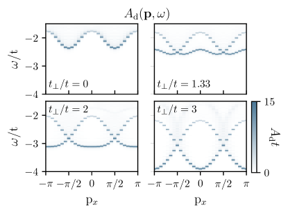
Figure 5: Polaron energy bands. The polaron energy bands along the diagonal ${\bf p}=(\mathrm{p}_{x},\mathrm{p}_{x})$ for $J/t=0.3$ and different values of $t_{\perp}$. This shows the splitting of the symmetric and anti-symmetric polaron energies when $t_{\perp}\neq 0$ except for $\mathbf{p}=\mathbf{Q}/2$ where the two states are degenerate. The momentum of the ground state also moves from $\mathbf{Q}$ to ${\mathbf{0}}$ with increasing $t_{\perp}$.

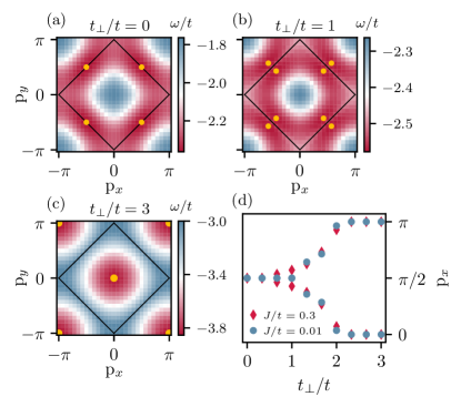
Figure 6: Magnetic polaron dispersion. Panel (a)-(c) show the energy of the magnetic polaron in the BZ for $J/t=0.3$ and $t_{\perp}/t=0,1,3$. The yellow dots indicate the minima and the black square the edge of the magnetic BZ given by $|{\mathrm{p}}_{x}|+|{\mathrm{p}}_{y}|=\pi$. Panel (d) shows the momentum $\mathbf{p}=(\mathrm{p}_{x},\mathrm{p}_{x})$ of the ground state as a function of $t_{\perp}/t$ for $J/t=0.01$ and $J/t=0.3$. Note that the mirror symmetry around the boundary of the magnetic BZ gives rise to several degenerate minima of the polaron energy.

VI Non-equilibrium dynamics

Having explored the fundamental equilibrium properties of a hole in the AF bilayer, we now turn to the non-equilibrium dynamics, which can be probed with unprecedented resolution in a new generation of optical lattice experiments Chiu et al. (2019); Brown et al. (2019); Koepsell et al. (2019); Ji et al. (2021); Koepsell et al. (2021); Gall et al. (2021); Hirthe et al. (2022).

We imagine a hole created at a given lattice site and analyze its subsequent dynamics. The key object to calculate for this kind of experiment is the Green’s function $G_{lm}^{>}({\mathbf{p}},\tau)=-i\langle\hat{h}_{l,{\mathbf{p}}}(\tau)\hat{h}^{\dagger}_{m,{\mathbf{p}}}(0)\rangle$, which gives the overlap between an initial state corresponding to a hole with momentum ${\mathbf{p}}$ in layer $m$ at time $0$, and a state where the hole is in layer $l$ at time $\tau$, which should not be confused with the imaginary time. This, hereby, gives access to the full dynamics of the lowest order coefficient in the many-body wave function Nielsen et al. (2022). While one in general needs a formalism such as Keldysh Green’s functions to calculate non-equilibrium many-body physics, it turns out that we can obtain the hole dynamics from our SCBA calculation by analytic continuation. The reason is that for a single hole, we have $iG^{>}_{ll}({\bf p},\omega)={A}_{\rm d}({\bf p},\omega)$ and $iG^{>}_{l\neq m}({\bf p},\omega)={A}_{\rm o}({\bf p},\omega)$ Skou et al. (2021); Bruus and Flensberg (2004). Hence, we can obtain the real time dynamics by Fourier transforming the spectral functions $\mathrm{A_{{\rm d}/{\rm o}}}(\mathbf{p},\omega)$.

VI.1 Interlayer oscillations

As we saw above, the spectral function in general consists of two quasiparticle peaks and a many-body continuum. In analogy with what has been observed for a mobile impurity atoms in atomic gases Nielsen et al. (2019); Skou et al. (2021), the continuum eventually decoheres so that the long time dynamics is governed by polaron formation. As a result, the real-time Green’s function approaches

$$iG^{>}_{\text{d}/\text{o}}({\bf p},\tau)\to\frac{1}{2}\left(Z^{+}_{{\bf p}}e^{-i\varepsilon^{+}_{{\bf p}}\tau}\pm Z^{-}_{{\bf p}}e^{-i\varepsilon^{-}_{{\bf p}}\tau}\right)$$ (22)

for long times, $\tau\gg 1/t$. Hence,

$$|G^{>}_{\text{d}}({\bf p},\tau)| =\frac{Z^{+}_{{\bf p}}}{2}\sqrt{1+\left(\frac{Z^{-}_{{\bf p}}}{Z^{+}_{{\bf p}}}\right)^{2}+2\frac{Z^{-}_{{\bf p}}}{Z^{+}_{{\bf p}}}\cos{(\Delta\varepsilon_{{\bf p}}\tau)}}$$

$$|G^{>}_{\text{o}}({\bf p},\tau)| =\frac{Z^{+}_{{\bf p}}}{2}\sqrt{1+\left(\frac{Z^{-}_{{\bf p}}}{Z^{+}_{{\bf p}}}\right)^{2}-2\frac{Z^{-}_{{\bf p}}}{Z^{+}_{{\bf p}}}\cos{(\Delta\varepsilon_{{\bf p}}\tau)}},$$ (23)

with $\Delta\varepsilon_{{\bf p}}=\varepsilon^{+}_{{\bf p}}-\varepsilon^{-}_{{\bf p}}$ the energy difference between the symmetric and anti-symmetric polaron.

In Fig. 7, we plot the hole dynamics as described by $|G^{>}_{\text{d}}({\bf p},\tau)|$ and $|G^{>}_{\text{o}}({\bf p},\tau)|$ for different momenta ${\mathbf{p}}={(\mathrm{p}_{x},\mathrm{p}_{x})}$ along the BZ diagonal, taking $J/t=0.3$, $t_{\perp}/t=0.5$(a) and $t_{\perp}/t=1.5$(b).

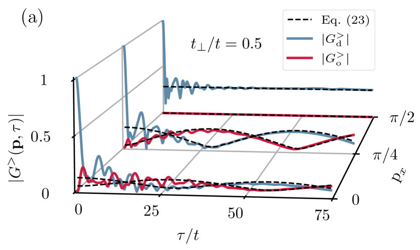
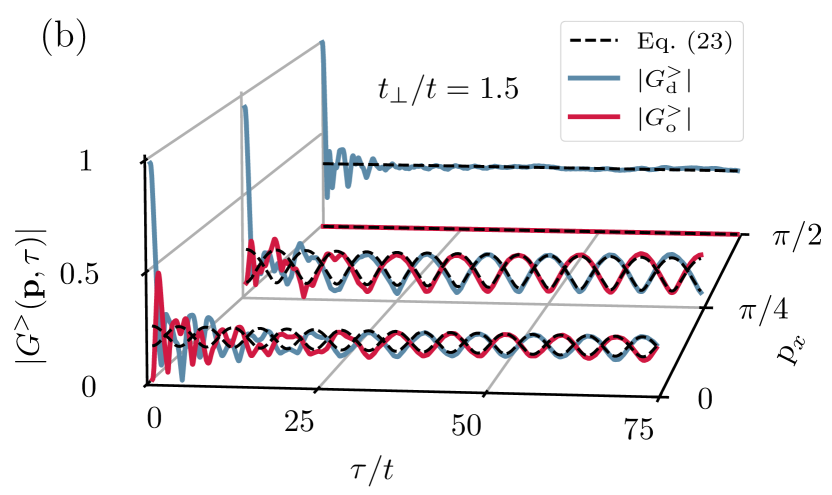
Figure 7: Hole oscillating between the layers. The diagonal and off-diagonal hole Green’s functions $G^{>}_{\rm d/o}({\bf p},\tau)$as a function of time for different momenta ${\mathbf{p}}=({\rm p}_{x},{\rm p}_{x})$. The long time prediction given by Eq. (23) is plotted as a dashed line.

Initially, $|G^{>}_{\text{d}}({\bf p},\tau)|$ decreases from unity simply reflecting that the hole starts to generate spin waves. On the other hand, $|G^{>}_{\text{o}}({\bf p},\tau)|$ increases from zero because the hole created in a given layer jumps to the other layer, except for ${\mathbf{p}}=(\pi/2,\pi/2)$ where it remains zero. The short time dynamics is, therefore, faster for $t_{\perp}/t=1.5$ than for $t_{\perp}/t=0.5$ as can be seen by comparing Figs. 7(a) and (b). At later times, the population of the hole is clearly seen to oscillate between the two layers, which is very accurately described by Eq. (23), confirming that the many-body continuum indeed decoheres for long times $\tau\gg t$. Physically, these oscillations arise from the fact that a hole initially localized in one layer corresponds to an equal superposition of the symmetric and anti-symmetric polaron. As time evolves, this results in a beating with a frequency given by their energy difference. The oscillations are faster for $t_{\perp}/t=1.5$ than for $t_{\perp}/t=0.5$, since a stronger coupling between the planes results in a larger energy splitting between the two polarons. There are, however, no oscillations for ${\mathbf{p}}={\mathbf{Q}}/2$ where the symmetric and anti-symmetric polarons are degenerate and the bare hole somewhat counterintuitively remains in one layer for all times. As discussed above, this is because the symmetric and anti-symmetric polarons are degenerate for ${\mathbf{p}}={\mathbf{Q}}/2$ so that a polaron eigenstate can be formed with the bare hole exclusively in one layer, while its presence in the other layer is always accompanied by spin waves. The excellent agreement between Eq. (23) and the numerics also illustrates that the dynamics of the bare hole and the polaron is strongly entangled, since Eq. (23) arises from only considering the polaron states whereas the Green’s functions give the dynamics of the bare hole.

Experimentally, this intriguing interlayer dynamics of the hole is most easily measured for the ${\mathbf{p}}=0$ case, since it corresponds to the hole initially being created with uniform density and no relative phase over one layer. The excited spin waves will change these oscillations, but using the form of the wave function in Eq. (13) shows that the oscillation frequency persists.

VI.2 Site resolved dynamics

In a recent optical lattice experiment, the motion of a hole initially created at a given lattice site was observed with single site resolution in a one AF layer Ji et al. (2021). Inspired by this impressive experiment, we now explore the hole dynamics in real space via the Green’s functions $G^{>}_{\text{d}}({\bf r},\tau)$ and $G^{>}_{\text{o}}({\bf r},\tau)$ obtained by Fourier transforming from momentum space. They give the overlap between an initial state with a hole created at the origin at time $0$, and a state where the hole is removed in the same/different layer at position ${\bf r}$ and time $\tau$.

In Fig. 8 we plot $|G^{>}_{\text{d}}({\bf r},\tau)|$ and $|G^{>}_{\text{o}}({\bf r},\tau)|$ for $J/t=0.3$ $t_{\perp}/t=0.67$, and $\tau/t=20$. One clearly sees how the hole has spread out, creating checkerboard patterns. These patterns are caused by the fact that the hole must jump an even number of times before the $\hat{{S}}^{+}_{l,\bf i}\hat{{S}}^{-}_{l,\bf j}$ terms in Eq. (3) can repair the magnetic frustration as discussed in Sec. V, and they are, therefore, inverted with respect to each other in the two layers. Figure 8, furthermore, shows that the expansion of the hole is faster along the diagonal directions. This is because the hole motion for long times is determined by the ballistic expansion of magnetic polarons Nielsen et al. (2022) as we will discuss further in Sec. VI.3. Since the polaron dispersion is steepest along the diagonals as can be seen in Fig. 6, this results in a faster expansion along those directions.

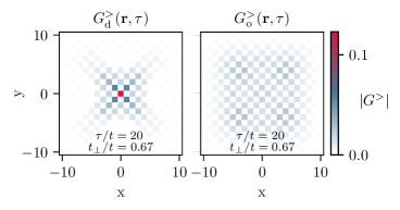
Figure 8: Real space hole dynamics. The diagonal and off-diagonal hole Green’s functions in real space for $t_{\perp}/t=0.67$, $J/t=0.3$ at time $\tau/t=20$.

We remind the reader that $G^{>}_{\text{d}/\text{o}}({\bf p},\tau)$ describes the dynamics of a bare hole in the sense that it gives the overlap between hole states separated by the time $\tau$ with no spin waves present. Hence, it does not give information regarding the overlap with final states describing the simultaneous presence of a hole and spin waves such as those connected to the origin by an odd number of jumps. As such, the checkerboard patterns shown in Fig. 8 is an artefact of projecting out these states. Nevertheless, the Green’s functions reflect the hole dynamics, since a bare hole is strongly entangled with the polarons. We discuss this point further in the next section.

VI.3 Order to disorder quantum phase transition

It is well-known that in the absence of a hole, the bilayer system undergoes a quantum phase transition with increasing $t_{\perp}/t$ from the ordered AF state to a disordered state, where neighbouring spins in the two layers form spin singlets Chubukov and Morr (1995); Scalettar et al. (1994); Millis and Monien (1994). Quantum Monte-Carlo calculations and series expansions yield the critical value $J_{\perp}/J\sim 2.5$ for this transition Hida (1992); Sandvik and Scalapino (1994); Sandvik et al. (1995), corresponding to $t_{\perp}/t=1.58$ when $J_{\perp}/J=t_{\perp}^{2}/t^{2}$. The presence of a single hole will not affect this phase transition, whereas the phase transition does affect the hole dynamics as we will now explore.

In Fig. 9, we plot the sublattice magnetization as a function of $t_{\perp}/t$ calculated within linear spin wave theory as

$$|\langle{S}^{z}\rangle|=\frac{1}{2}-\frac{1}{2N}\sum_{\mathbf{k}}\left(v_{\mathbf{k},+}^{2}+v_{\mathbf{k},-}^{2}\right).$$ (24)

The magnetization first increases with $t_{\perp}/t$ reaching a maximum at $t_{\perp}/t=0.82$ after which it decreases until magnetic order is lost at $t_{\perp}/t=3.67$ in agreement with Ref. Chubukov and Morr (1995). Linear spin wave theory thus captures the qualitative physics of the phase transition with the AF order going to zero, but as usual for a mean-field theory, it overestimates the transition point due to the omission of longitudinal spin fluctuations Chubukov and Morr (1995).

Figure 9: Magnetization and hole velocity. The sublattice magnetization given by Eq. (24) (black), and the final rms velocity of the hole (red). The magnetization shown is scaled such that unity corresponds to perfect AF alignment.

To explore the effects of this phase transition on the hole dynamics, we plot in Fig. 10 the diagonal and off-diagonal real space Green’s functions for $\tau/t=16$ and $\tau/t=22$. This shows that the hole delocalizes slower for $t_{\perp}/t=1$ compared to $t_{\perp}/t=0$. Physically, this is because the AF order is larger at $t_{\perp}/t=1$, see Fig. 9, making it energetically more costly for the hole to move. Increasing the interlayer coupling further, we see that the hole delocalizes faster for $t_{\perp}/t=3$. This non-monotonic behaviour of the hole expansion velocity is consistent with the magnetic order, which first increases with increasing interlayer coupling before it vanishes at the phase transition.

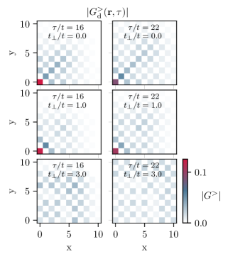
Figure 10: Hole expansion for different interlayer couplings. The real space diagonal hole Green’s function for $J/t=0.3$, $t_{\perp}/t=0,1,3$, and $\tau/t=15,22$.

To quantify this, we consider the rms distance of the bare hole from origin defined by

$$d_{\mathrm{rms}}(\tau)=\sqrt{\frac{\sum_{{\bf r}}r^{2}\left(|G^{>}_{\rm d}({\bf r},\tau)|^{2}+|G^{>}_{\rm o}({\bf r},\tau)|^{2}\right)}{\sum_{{\bf r}}\left(|G^{>}_{\rm d}({\bf r},\tau)|^{2}+|G^{>}_{\rm o}({\bf r},\tau)|^{2}\right)}}.$$ (25)

The normalization takes care of the fact that the likelihood of finding a bare hole is less than unity for $\tau>0$ where spin waves are present. Indeed, we have $\sum_{{\bf r}}(|G^{>}_{\rm d}({\bf r},\tau)|^{2}+|G^{>}_{\rm o}({\bf r},\tau)|^{2})\rightarrow\sum_{\bf{p}}(({Z^{+}_{\bf{p}}})^{2}+({Z^{-}_{\bf{p}}})^{2})/2N$ for $\tau/t\rightarrow\infty$ when the many-body continuum has decohered.

In Fig. 11, we plot $d_{\mathrm{rms}}(\tau)$ for $J/t=0.3$ and $t_{\perp}/t=0,1,2,3$. After an initial rapid expansion and oscillations, the hole starts moving with a constant velocity. This long time dynamics of the hole is governed by ballistic expansion of magnetic polarons, which have been formed after the initial creation of a bare hole. Indeed, it has recently been shown using a time-dependent wave function within the SCBA that the long time expansion of a hole initially created at a given site in a single layer is determined by the formation and ballistic motion of magnetic polarons Nielsen et al. (2022). Here, we find $v_{\text{rms}}=\dot{d}_{\text{rms}}=0.213t$ for the expansion velocity of the bare hole at long times in the case of the two layers completely decoupled with $t_{\perp}/t=0$. This is very close to value $v_{\mathrm{rms}}=0.215t$ found for the final expansion velocity of magnetic polarons for a single layer Nielsen et al. (2022). The agreement explicitly demonstrates that the motion of the bare hole discussed in this paper closely follows the motion of magnetic polarons for long times, which can be understood from the fact that the hole is closely entangled with the polaron for long times.

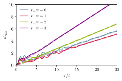
Figure 11: rms distance of the hole. The rms distance given by Eq. 25 for $J/t=0.3$ and $t_{\perp}/t=0,1,2,3$. The final expansion velocities are in Fig. 9 are found from the slopes of the asymptotic dashed lines.

Figure 11, furthermore, shows that the hole expands slower for $t_{\perp}/t=1$ as compared to $t_{\perp}/t=0$, and that the expansion velocity then increases again with $t_{\perp}/t=3$, consistent with Fig. 10. This is illustrated further in Fig. 9 where the final expansion velocity after the magnetic polaron has formed is plotted as a function of $t_{\perp}/t$. The expansion velocity depends non-monotonically on $t_{\perp}/t=0$, directly reflecting the behaviour of the magnetic order also shown in Fig. 9. From this we conclude that the approach to the order-to-disorder phase transition of the bilayer system with increasing interlayer coupling can be detected as an increase in the hole expansion velocity as the transition point is approached from the AF phase, reflecting the decrease in the magnetic energy cost of hole hopping.

It should be noted that while our theory does not contain the singlet correlations across the layers giving rise to the disordered phase, we believe our results are qualitatively reliable. In particular, the increase in the expansion velocity as the phase transition is approached inside the AF phase is a robust result, since a decreasing magnetic order means less energy cost for hole hopping, which physically must be expected to lead to a higher velocity. Also, our theory agrees qualitatively with a variational calculation interpolating between the ordered AF state and a disordered singlet product state regarding the influence of the interlayer coupling on the polaron spectrum Vojta and Becker (1999). In this paper, the momentum of the ground state was also predicted to move from ${\mathbf{Q}}/2$ to ${\mathbf{0}}$ with increasing interlayer coupling $J_{\perp}$ in agreement with our findings shown in Fig. 6. Band structures similar to what we show in Fig. 5 were also reported. So even though our analysis for the phase transition is quantitatively unreliable, we expect the main finding, i.e. the speed up of the hole, to be qualitatively correct.

VII Conclusions

We investigated the equilibrium and non-equilibrium properties of a hole in an AF bilayer using a diagrammatic approach based on the SCBA. The spectral properties of the hole were shown to exhibit two quasiparticle peaks corresponding to magnetic polarons that are either symmetric or anti-symmetric under layer exchange. We calculated the energy bands of these two kinds of polarons in the BZ and showed that they are degenerate at certain momenta due to the underlying AF symmetry. The momentum of the ground state polaron was, furthermore, shown to move to the origin of the BZ with increasing interlayer coupling. We then demonstrated that a hole initially created in one layer, oscillates between the two layers with a frequency determined by the energy difference between the symmetric and the anti-symmetric polaron. Finally, we analyzed how the asymptotic expansion velocity of a hole initially created at a given lattice site is governed by the ballistic motion of polarons, and that it first decreases and then increases as a function of the interlayer coupling, reflecting that a quantum phase transition to a disordered state of the spins is approached.

We have largely focuzed on observables that are accessible in experiments based on cold atoms in optical lattices. In particular, their single site resolution and the ability to perform quench experiments where a hole is abruptly released from a given lattice site Chiu et al. (2019); Brown et al. (2019); Koepsell et al. (2019); Ji et al. (2021); Koepsell et al. (2021), combined with the recent creation of a bilayer system Gall et al. (2021), show that optical lattices provide a promising platform to observe the effects discussed above.

Interesting future research directions include calculating the time-dependent wave function of a hole initially created at a given lattice in the bilayer using the SCBA. This has recently been achieved for a single layer Nielsen et al. (2022) and would give access to the full non-equilibrium dynamics of the hole. Another intriguing question concerns the properties of a hole in the disordered phase for large interlayer coupling, where neighbouring spins in the two layers form singlets. Finally, an important problem concerns the role of temperature, since optical lattice experiments invariably are performed at a non-zero temperature.

Acknowledgments.- This work has been supported by the Danish National Research Foundation through the Center of Excellence ”CCQ” (Grant agreement no.: DNRF156), as well as the Carlsberg Foundation through a Carlsberg Internationalisation Fellowship. We thank T. Pohl for useful comments and discussions.

Appendix A Diagonalization of $\hat{H}_{J}$

In this appendix, we will elaborate on the steps taken in diagonalizing $\hat{H}_{J}$, Eq. (3). Using the mappings described in Section II and neglecting the hardcore constraint we find

$$\hat{H}_{J}= \ \hat{H}^{int}_{J}+\frac{J}{2}\sum_{\langle{\bf i}{\bf j}\rangle,l}\Big{[}\hat{s}^{\dagger}_{l,{\bf i}}\hat{s}_{l,{\bf i}}+\hat{s}^{\dagger}_{l,{\bf j}}\hat{s}_{l,{\bf j}}$$

$$+\alpha\left(\hat{s}_{l,{\bf i}}\hat{s}_{l,{\bf j}}+\hat{s}^{\dagger}_{l,{\bf j}}\hat{s}^{\dagger}_{l,{\bf i}}\right)\Big{]}-\frac{Jz}{2}\left(N-1\right)$$

$$+\frac{J_{\perp}}{2}\sum_{i}\Big{[}\hat{s}^{\dagger}_{l,{\bf i}}\hat{s}_{l,{\bf i}}+\hat{s}^{\dagger}_{\bar{l},{\bf i}}\hat{s}_{\bar{l},{\bf i}}$$

$$+\alpha_{\perp}\left(\hat{s}_{l,{\bf i}}\hat{s}_{\bar{l},{\bf i}}+\hat{s}^{\dagger}_{\bar{l},{\bf i}}\hat{s}^{\dagger}_{l,{\bf i}}\right)\Big{]}-\frac{J_{\perp}}{2}\left(N-1\right),$$ (26)

where $\hat{H}^{int}_{J}$ contains the non-linear terms which are neglected. $\alpha$ and $\alpha_{\perp}$ describe possible intra and inter layer anisotropy respectively. They are set equal to unity in the main text for the sake of clarity, but they can easily be considered. Defining the Fourier transform in the standard way

$$\hat{s}_{l,{\bf i}}=\frac{1}{\sqrt{N}}\sum_{\textbf{k}}e^{i\textbf{k}\cdot{\bf i}}\hat{s}_{l,\textbf{k}},$$ (27)

the Hamiltonian in momentum space can be written as

$$\hat{H}^{int}_{J}=E_{0}+\frac{1}{4}\sum_{\textbf{k}}$$

$$\begin{bmatrix}\hat{s}^{\dagger}_{1,\textbf{k}}&\hat{s}_{1,-\textbf{k}}&\hat{s}^{\dagger}_{2,\textbf{k}}&\hat{s}_{2,-\textbf{k}}\end{bmatrix}\begin{bmatrix}\mathcal{H}_{\rm d}&\mathcal{H}_{\rm o}\\ \mathcal{H}_{\rm o}&\mathcal{H}_{\rm d}\end{bmatrix}\begin{bmatrix}\hat{s}_{1,\textbf{k}}\\ \hat{s}^{\dagger}_{1,-\textbf{k}}\\ \hat{s}_{2,\textbf{k}}\\ \hat{s}^{\dagger}_{2,-\textbf{k}}\end{bmatrix}$$

with

$$\mathcal{H}_{\rm d} =\begin{bmatrix}Jz+J_{\perp}&\alpha Jz\gamma_{\textbf{k}}\\ \alpha Jz\gamma_{\textbf{k}}&Jz+J_{\perp}\end{bmatrix}$$

$$\mathcal{H}_{\rm o} =\begin{bmatrix}0&\alpha_{\perp}J_{\perp}\\ \alpha_{\perp}J_{\perp}&0\end{bmatrix}.$$ (29)

To diagonalize a Hamiltoninan of this kind, it is practical to get it on a block diagonal form first by performing a unitary transformation. In the block diagonal form, one can then utilize the canonical Bogoliubov transformation for each block individually. To do so, we realize

$$\frac{1}{2}\begin{bmatrix}\mathds{1}_{2}&\mathds{1}_{2}\\ -\mathds{1}_{2}&\mathds{1}_{2}\end{bmatrix}\begin{bmatrix}\mathcal{H}_{\rm d}&\mathcal{H}_{\rm o}\\ \mathcal{H}_{\rm o}&\mathcal{H}_{\rm d}\end{bmatrix}\begin{bmatrix}\mathds{1}_{2}&-\mathds{1}_{2}\\ \mathds{1}_{2}&\mathds{1}_{2}\end{bmatrix}=$$

$$\begin{bmatrix}\mathcal{H}_{\rm d}+\mathcal{H}_{\rm o}&0\\ 0&\mathcal{H}_{\rm d}-\mathcal{H}_{\rm o}\end{bmatrix},$$ (30)

such that by defining

$$\begin{bmatrix}\hat{s}_{1,{\bf k}}\\ \hat{s}^{\dagger}_{1,-{\bf k}}\\ \hat{s}_{2,{\bf k}}\\ \hat{s}^{\dagger}_{2,-{\bf k}}\end{bmatrix}=\frac{1}{\sqrt{2}}\begin{bmatrix}\mathds{1}_{2}&-\mathds{1}_{2}\\ \mathds{1}_{2}&\mathds{1}_{2}\end{bmatrix}\begin{bmatrix}U_{+,{\bf k}}&0\\ 0&U_{-,{\bf k}}\end{bmatrix}\begin{bmatrix}\hat{b}_{+,{\bf k}}\\ \hat{b}^{\dagger}_{+,-{\bf k}}\\ \hat{b}_{-,{\bf k}}\\ \hat{b}^{\dagger}_{-,-{\bf k}}\end{bmatrix}.$$ (31)

and choosing

$$U_{\pm,{\bf k}}=\begin{bmatrix}u_{\pm,{\bf k}}&-v_{\pm,{\bf k}}\\ -v_{\pm,{\bf k}}&u_{\pm,{\bf k}}\end{bmatrix}$$ (32)

with the coherence factors given by

$$u_{\pm,{\bf k}} =\sqrt{\frac{1}{2}\left(\frac{zJ+J_{\perp}}{2\omega_{\pm,{\bf k}}}+1\right)},$$

$$v_{\pm,{\bf k}} ={\rm sgn}\left[\alpha zJ\gamma_{\bf k}\pm\alpha_{\perp}J_{\perp}\right]\sqrt{\frac{1}{2}\left(\frac{zJ+J_{\perp}}{2\omega_{\pm,{\bf k}}}-1\right)}$$ (33)

the Hamiltonian becomes diagonal

$$\hat{H}_{J}\simeq E_{0}+\sum_{{\bf k},\mu=\pm}\omega_{\mu,{\bf k}}\hat{b}^{\dagger}_{\mu,{\bf k}}\hat{b}_{\mu,{\bf k}},$$ (34)

with the dispersion relations

$$\omega_{\pm,{\bf k}}=\frac{1}{2}\sqrt{\left(Jz+J_{\perp}\right)^{2}-\left(\alpha Jz\gamma_{{\bf k}}\pm\alpha_{\perp}J_{\perp}\right)^{2}}.$$ (35)

Appendix B Sum rule for $A_{{\rm o}}$

By following the same approach as presented in Bruus and Flensberg (2004) it is shown that

$$\int_{-\infty}^{\infty}\frac{\text{d}\omega}{2\pi}{A}_{\rm o}({\bf p},\omega)=0.$$ (36)

From the definition of the off-diagonal spectral function

$$\int_{-\infty}^{\infty}\frac{\text{d}\omega}{2\pi}{A}_{\rm o}({\bf p},\omega) =-\int_{-\infty}^{\infty}\frac{\text{d}\omega}{2\pi}2\text{Im}[G^{R}_{\rm o}({\bf p},\omega)].$$ (37)

As shown in Bruus and Flensberg (2004) for the diagonal part, one can by using the Lehmann representation state the imaginary part of the retarded Green’s function as

$$2\text{Im}[G^{R}_{\rm o}({\bf p},\omega)]= -\frac{2\pi}{Z}\sum_{n,n^{\prime}}\bra{n}\hat{h}_{2,{\bf p}}\ket{n^{\prime}}\bra{n^{\prime}}\hat{h}_{1,{\bf p}}^{\dagger}\ket{n}$$

$$\left(e^{-\beta\rm{E_{n}}}+e^{-\beta\rm{E_{n^{\prime}}}}\right)\delta(\omega+\rm{E_{n}}-\rm{E_{n^{\prime}}}),$$ (38)

where $Z$ is a normalization constant defined such that $\left\langle...\right\rangle=\sum_{n}\bra{n}e^{-\beta\mathrm{\hat{H}}}...\ket{n}/Z$, and the summation runs over all states with no holes present. Inserting this expression into Eq. (37) we find

$$\int_{-\infty}^{\infty}\frac{\text{d}\omega}{2\pi}{A}_{\rm o}({\bf p},\omega)= \ \frac{1}{Z}\sum_{n,n^{\prime}}\bra{n}\hat{h}_{{\bf p},2}\ket{n^{\prime}}\bra{n^{\prime}}\hat{h}_{{\bf p},1}^{\dagger}\ket{n}$$

$$\ \left(e^{-\beta\rm{E_{n}}}+e^{-\beta\rm{E_{n^{\prime}}}}\right)$$

$$= \ \frac{1}{Z}\sum_{n,n^{\prime}}\Big{(}\bra{n}\hat{h}_{2,{\bf p}}\ket{n^{\prime}}\bra{n^{\prime}}\hat{h}_{1,{\bf p}}^{\dagger}\ket{n}e^{-\beta\rm{E_{n}}}$$

$$\ +\bra{n^{\prime}}\hat{h}_{1,{\bf p}}^{\dagger}\ket{n}\bra{n}\hat{h}_{2,{\bf p}}\ket{n^{\prime}}e^{-\beta\rm{E_{n^{\prime}}}}\Big{)}$$

$$= \ \frac{1}{Z}\sum_{n}\Big{(}\bra{n}\hat{h}_{2,{\bf p}}\hat{h}_{1,{\bf p}}^{\dagger}\ket{n}e^{-\beta\rm{E_{n}}}$$

$$\ +\bra{n}\hat{h}_{1,{\bf p}}^{\dagger}\hat{h}_{2,{\bf p}}\ket{n}e^{-\beta\rm{E_{n}}}\Big{)}$$

$$= \ \left\langle\hat{h}_{2,{\bf p}}\hat{h}_{1,{\bf p}}^{\dagger}+\hat{h}_{1,{\bf p}}^{\dagger}\hat{h}_{2,{\bf p}}\right\rangle$$

$$= \ 0.$$ (39)

References

- Keimer et al. (2015) B. Keimer, S. A. Kivelson, M. R. Norman, S. Uchida, and J. Zaanen, “From quantum matter to high-temperature superconductivity in copper oxides,” Nature 518, 179–186 (2015).
- Wen and Li (2011) Hai-Hu Wen and Shiliang Li, “Materials and novel superconductivity in iron pnictide superconductors,” Annual Review of Condensed Matter Physics 2, 121–140 (2011), https://doi.org/10.1146/annurev-conmatphys-062910-140518 .
- Wosnitza (2012) Jochen Wosnitza, “Superconductivity in layered organic metals,” Crystals 2, 248–265 (2012).
- Cao et al. (2018) Yuan Cao, Valla Fatemi, Shiang Fang, Kenji Watanabe, Takashi Taniguchi, Efthimios Kaxiras, and Pablo Jarillo-Herrero, “Unconventional superconductivity in magic-angle graphene superlattices,” Nature 556, 43–50 (2018).
- Dagotto (1994) Elbio Dagotto, “Correlated electrons in high-temperature superconductors,” Rev. Mod. Phys. 66, 763–840 (1994).
- Lee et al. (2006) Patrick A. Lee, Naoto Nagaosa, and Xiao-Gang Wen, “Doping a mott insulator: Physics of high-temperature superconductivity,” Rev. Mod. Phys. 78, 17–85 (2006).
- Damascelli et al. (2003) Andrea Damascelli, Zahid Hussain, and Zhi-Xun Shen, “Angle-resolved photoemission studies of the cuprate superconductors,” Rev. Mod. Phys. 75, 473–541 (2003).
- Schmitt-Rink et al. (1988) S. Schmitt-Rink, C. M. Varma, and A. E. Ruckenstein, “Spectral Function of Holes in a Quantum Antiferromagnet,” Physical Review Letters 60, 2793–2796 (1988).
- Shraiman and Siggia (1988) Boris I. Shraiman and Eric D. Siggia, “Mobile Vacancies in a Quantum Heisenberg Antiferromagnet,” Physical Review Letters 61, 467–470 (1988).
- Kane et al. (1989) C. L. Kane, P. A. Lee, and N. Read, “Motion of a single hole in a quantum antiferromagnet,” Physical Review B 39, 6880–6897 (1989).
- Martinez and Horsch (1991) Gerardo Martinez and Peter Horsch, “Spin polarons in the t - J model,” Physical Review B 44, 317–331 (1991).
- Liu and Manousakis (1991) Zhiping Liu and Efstratios Manousakis, “Spectral function of a hole in the t - J model,” Physical Review B 44, 2414–2417 (1991).
- Marsiglio et al. (1991) Frank Marsiglio, Andrei E. Ruckenstein, Stefan Schmitt-Rink, and Chandra M. Varma, “Spectral function of a single hole in a two-dimensional quantum antiferromagnet,” Physical Review B 43, 10882–10889 (1991).
- Chernyshev and Leung (1999) A. L. Chernyshev and P. W. Leung, “Holes in the t - J z model: A diagrammatic study,” Physical Review B 60, 1592–1606 (1999).
- Diamantis and Manousakis (2021) Nikolaos G Diamantis and Efstratios Manousakis, “Dynamics of string-like states of a hole in a quantum antiferromagnet: a diagrammatic monte carlo simulation,” New Journal of Physics 23, 123005 (2021).
- Nielsen et al. (2022) K. Knakkergaard Nielsen, T. Pohl, and G. M. Bruun, “Non-equilibrium hole dynamics in antiferromagnets: Damped strings and polarons,” arXiv:2203.04789v1 [cond-mat.quant-gas] (2022), 10.48550/arXiv.2203.04789, arXiv:2203.04789v1 [cond-mat.quant-gas] .
- Nazarenko and Dagotto (1996) Alexander Nazarenko and Elbio Dagotto, “Hole dispersion and symmetry of the superconducting order parameter for underdoped CuO 2 bilayers and the three-dimensional antiferromagnets,” Physical Review B 54, 13158–13166 (1996).
- Yin and Gong (1997) Wei-Guo Yin and Chang-De Gong, “Quasiparticle bands in the realistic bilayer cuprates,” Physical Review B 56, 2843–2846 (1997).
- Yin and Gong (1998) Wei-Guo Yin and Chang-De Gong, “Quasiparticle bands and superconductivity for the multiple-layer and three-dimensional superlattice t - J models,” Physical Review B 57, 11743–11751 (1998).
- Hida (1992) Kazuo Hida, “Quantum disordered state without frustration in the double layer heisenberg antiferromagnet –dimer expansion and projector monte carlo study–,” Journal of the Physical Society of Japan 61, 1013–1018 (1992), https://doi.org/10.1143/JPSJ.61.1013 .
- Sandvik and Scalapino (1994) A. W. Sandvik and D. J. Scalapino, “Order-disorder transition in a two-layer quantum antiferromagnet,” Phys. Rev. Lett. 72, 2777–2780 (1994).
- Scalettar et al. (1994) Richard T. Scalettar, Joel W. Cannon, Douglas J. Scalapino, and Robert L. Sugar, “Magnetic and pairing correlations in coupled Hubbard planes,” Physical Review B 50, 13419–13427 (1994).
- Millis and Monien (1994) A. J. Millis and H. Monien, “Spin gaps and bilayer coupling in YBa 2 Cu 3 O 7 - and YBa 2 Cu 4 O 8,” Physical Review B 50, 16606–16622 (1994).
- Sandvik et al. (1995) Anders W. Sandvik, Andrey V. Chubukov, and Subir Sachdev, “Quantum critical behavior in a two-layer antiferromagnet,” Phys. Rev. B 51, 16483–16486 (1995).
- Chubukov and Morr (1995) Andrey V. Chubukov and Dirk K. Morr, “Phase transition, longitudinal spin fluctuations, and scaling in a two-layer antiferromagnet,” Physical Review B 52, 3521–3532 (1995).
- Carlström et al. (2016) Johan Carlström, Nikolay Prokof’ev, and Boris Svistunov, “Quantum walk in degenerate spin environments,” Phys. Rev. Lett. 116, 247202 (2016).
- Kanász-Nagy et al. (2017) Márton Kanász-Nagy, Izabella Lovas, Fabian Grusdt, Daniel Greif, Markus Greiner, and Eugene A. Demler, “Quantum correlations at infinite temperature: The dynamical nagaoka effect,” Phys. Rev. B 96, 014303 (2017).
- Grusdt et al. (2018a) Fabian Grusdt, Zheng Zhu, Tao Shi, and Eugene Demler, “Meson formation in mixed-dimensional t-J models,” SciPost Physics 5, 057 (2018a).
- Grusdt et al. (2018b) F. Grusdt, M. Kánasz-Nagy, A. Bohrdt, C. S. Chiu, G. Ji, M. Greiner, D. Greif, and E. Demler, “Parton theory of magnetic polarons: Mesonic resonances and signatures in dynamics,” Phys. Rev. X 8, 011046 (2018b).
- Nielsen et al. (2021) K. K. Nielsen, M. A. Bastarrachea-Magnani, T. Pohl, and G. M. Bruun, “Spatial structure of magnetic polarons in strongly interacting antiferromagnets,” Physical Review B 104, 155136 (2021).
- Chiu et al. (2019) Christie S. Chiu, Geoffrey Ji, Annabelle Bohrdt, Muqing Xu, Michael Knap, Eugene Demler, Fabian Grusdt, Markus Greiner, and Daniel Greif, “String patterns in the doped hubbard model,” Science 365, 251–256 (2019), https://www.science.org/doi/pdf/10.1126/science.aav3587 .
- Brown et al. (2019) Peter T. Brown, Debayan Mitra, Elmer Guardado-Sanchez, Reza Nourafkan, Alexis Reymbaut, Charles-David Hébert, Simon Bergeron, A.-M. S. Tremblay, Jure Kokalj, David A. Huse, Peter Schauß, and Waseem S. Bakr, “Bad metallic transport in a cold atom fermi-hubbard system,” Science 363, 379–382 (2019), https://www.science.org/doi/pdf/10.1126/science.aat4134 .
- Koepsell et al. (2019) Joannis Koepsell, Jayadev Vijayan, Pimonpan Sompet, Fabian Grusdt, Timon A. Hilker, Eugene Demler, Guillaume Salomon, Immanuel Bloch, and Christian Gross, “Imaging magnetic polarons in the doped fermi–hubbard model,” Nature 572, 358–362 (2019).
- Ji et al. (2021) Geoffrey Ji, Muqing Xu, Lev Haldar Kendrick, Christie S. Chiu, Justus C. Brüggenjürgen, Daniel Greif, Annabelle Bohrdt, Fabian Grusdt, Eugene Demler, Martin Lebrat, and Markus Greiner, “Coupling a mobile hole to an antiferromagnetic spin background: Transient dynamics of a magnetic polaron,” Phys. Rev. X 11, 021022 (2021).
- Koepsell et al. (2021) Joannis Koepsell, Dominik Bourgund, Pimonpan Sompet, Sarah Hirthe, Annabelle Bohrdt, Yao Wang, Fabian Grusdt, Eugene Demler, Guillaume Salomon, Christian Gross, and Immanuel Bloch, “Microscopic evolution of doped mott insulators from polaronic metal to fermi liquid,” Science 374, 82–86 (2021), https://www.science.org/doi/pdf/10.1126/science.abe7165 .
- Gall et al. (2021) Marcell Gall, Nicola Wurz, Jens Samland, Chun Fai Chan, and Michael Köhl, “Competing magnetic orders in a bilayer Hubbard model with ultracold atoms,” Nature 589, 40–43 (2021).
- Hirthe et al. (2022) Sarah Hirthe, Thomas Chalopin, Dominik Bourgund, Petar Bojović, Annabelle Bohrdt, Eugene Demler, Fabian Grusdt, Immanuel Bloch, and Timon A. Hilker, “Magnetically mediated hole pairing in fermionic ladders of ultracold atoms,” (2022).
- Chao et al. (1977) K A Chao, J Spalek, and A M Oles, “Kinetic exchange interaction in a narrow s-band,” Journal of Physics C: Solid State Physics 10, L271–L276 (1977).
- Reischl et al. (2004) Alexander Reischl, Erwin Müller-Hartmann, and Götz S. Uhrig, “Systematic mapping of the Hubbard model to the generalized t - J model,” Physical Review B 70, 245124 (2004).
- Koepsell et al. (2020) Joannis Koepsell, Sarah Hirthe, Dominik Bourgund, Pimonpan Sompet, Jayadev Vijayan, Guillaume Salomon, Christian Gross, and Immanuel Bloch, “Robust Bilayer Charge Pumping for Spin- and Density-Resolved Quantum Gas Microscopy,” Physical Review Letters 125, 010403 (2020).
- Browaeys and Lahaye (2020) Antoine Browaeys and Thierry Lahaye, “Many-body physics with individually controlled rydberg atoms,” Nature Physics 16, 132–142 (2020).
- Reiter (1994) George F. Reiter, “Self-consistent wave function for magnetic polarons in the t - J model,” Physical Review B 49, 1536–1539 (1994).
- Ramšak and Horsch (1998) A. Ramšak and P. Horsch, “Spatial structure of spin polarons in the t - J model,” Physical Review B 57, 4308–4320 (1998).
- Ramsak and Horsch (1993) A Ramsak and P Horsch, “Spin polarons in the t-J model: Shape and backflow,” Physical Review B 48, 4 (1993).
- Liu and Manousakis (1992) Zhiping Liu and Efstratios Manousakis, “Dynamical properties of a hole in a Heisenberg antiferromagnet,” Physical Review B 45, 2425–2437 (1992).
- Vojta and Becker (1999) Matthias Vojta and Klaus W. Becker, “Doped bilayer antiferromagnets: Hole dynamics on both sides of a magnetic ordering transition,” Physical Review B 60, 15201–15213 (1999).
- Skou et al. (2021) Magnus G. Skou, Thomas G. Skov, Nils B. Jørgensen, Kristian K. Nielsen, Arturo Camacho-Guardian, Thomas Pohl, Georg M. Bruun, and Jan J. Arlt, “Non-equilibrium quantum dynamics and formation of the Bose polaron,” Nature Physics 17, 731–735 (2021).
- Bruus and Flensberg (2004) Henrik Bruus and Karsten Flensberg, Many-Body Quantum Theory in Condensed Matter Physics: An Introduction, Oxford Graduate Texts (Oxford University Press, Oxford ; New York, 2004).
- Nielsen et al. (2019) K Knakkergaard Nielsen, L A Peña Ardila, G M Bruun, and T Pohl, “Critical slowdown of non-equilibrium polaron dynamics,” New Journal of Physics 21, 043014 (2019).