The first catalogue of spectroscopically confirmed red nuggets
at z$\sim$0.7 from the VIPERS survey

Abstract

Context. ’Red nuggets’ are a rare population of passive compact massive galaxies thought to be the first massive galaxies that formed in the Universe. First found at $z\sim 3$, they are even less abundant at lower redshifts, and it is believed that with time they mostly transformed through mergers into today’s giant ellipticals. Those red nuggets which managed to escape this fate can serve as unique laboratories to study the early evolution of massive galaxies.

Aims. In this paper, we aim to make use of the unprecedented statistical power of the VIMOS Public Extragalactic Redshift Survey to build the largest up-to-date catalogue of spectroscopically confirmed red nuggets at the intermediate redshift $0.5<z<1.0$.

Methods. Starting from a catalogue of nearly 90 000 VIPERS galaxies we select sources with stellar masses $M_{star}>8\times 10^{10}$ $\rm{M}_{\odot}$ and effective radii $R_{\mathrm{e}}<1.5$ kpc. Among them, we select red, passive galaxies with old stellar population based on colour–colour NUVrK diagram, star formation rate values, and verification of their optical spectra.

Results. Verifying the influence of the limit of the source compactness on the selection, we found that the sample size can vary even up to two orders of magnitude, depending on the chosen criterion. Using one of the most restrictive criteria with additional checks on their spectra and passiveness, we spectroscopically identified only 77 previously unknown red nuggets. The resultant catalogue of 77 red nuggets is the largest such catalogue built based on the uniform set of selection criteria above the local Universe. Number density calculated on the final sample of 77 VIPERS passive red nuggets per comoving Mpc³ increases from 4.7$\times 10^{-6}$ at $z\sim 0.61$ to $9.8\times 10^{-6}$ at $z\sim 0.95$, which is higher than values estimated in the local Universe, and lower than the ones found at $z>2$. It fills the gap at intermediate redshift.

Conclusions. A catalogue of red nuggets presented in this paper is a golden sample for future studies of this rare population of objects at intermediate redshift. Besides covering a unique redshift range and careful selection of galaxies, the catalogue is spectroscopically identified.

1 Introduction

Morphological classification of galaxies splits them into two main groups, early and late types (Hubble 1926). The early-type galaxies (ETGs) are spheroidal objects with smooth brightness distributions, low star formation (SF) rates, and stellar content dominated by evolved stars. The late-type galaxies are at the opposite side of Hubble’s tuning fork diagram: those are mostly spiral galaxies and contain both young and evolved stars (Kennicutt 1998).

It has been shown that the most massive ETGs in the local Universe differ significantly from their counterparts at high redshifts ($z>2$). These high-redshift ETGs are extremely compact, a few times smaller in size than their local counterparts Daddi et al. (2005); Trujillo et al. (2007); Damjanov et al. (2009); van der Wel et al. (2014). According to the so-called two-phase formation scenario, during the initial phase dominated by numerous wet mergers between gas-rich galaxies and characterized by high star formation rate (SFR), progenitors of ETGs increase their stellar mass rapidly, even up to $M_{star}\sim 10^{11}$ M_⊙, but remain compact in size (Oser et al. 2010). Subsequently, star formation in these compact and massive objects quenches quickly, and the galaxies become passive, compact, and massive. At this stage, those are referred to as a ‘red nuggets’. In the second, final phase, red nuggets undergo dry mergers with other gas-poor galaxies which results in the increase of their size and their transformation in giant elliptical galaxies (van Dokkum et al. 2010). This two-phase scenario has been confirmed observationally (Barro et al. 2013; Zibetti et al. 2020), and is predicted by theoretical models and numerical simulations (Naab et al. 2009; Zolotov et al. 2015; Flores-Freitas et al. 2021).

Due to the stochastic nature of mergers, some red nuggets skip the second phase of the two-phase scenario and end as so-called ‘relics’ (Ferré-Mateu et al. 2017). Red nuggets (relics) provide a unique opportunity to study stellar populations that remained relatively unaltered for billions of years. Yet, direct observational studies of red nuggets have been cursory so far due to their high-redshift and the lack of sufficient angular resolution. Moreover, the probability of finding the relics in the local Universe is very low, as most of them already merged. The high-resolution cosmological simulations predict that the fraction of $z\sim 2$ red nuggets that evolve into local Universe relics is less than 15% (Quilis & Trujillo 2013; Wellons et al. 2016; Furlong et al. 2017). These predictions vary depending on the exact description of physical processes influencing the galaxy evolution, in particular stellar winds or Active Galaxy Nuclei (AGN) feedback, in the simulations.

Despite numerous observational studies dedicated to identifying relics at the lowest redshifts, $z\leq 0.2$, their estimated number densities differ by a few orders of magnitude between different samples (Trujillo et al. 2009; Taylor et al. 2010; Valentinuzzi et al. 2010; Poggianti et al. 2013; Saulder et al. 2015; Tortora et al. 2016; Ferré-Mateu et al. 2017; Scognamiglio et al. 2020). A likely reason for these differences is different selection criteria for compact sources applied by the authors. At redshifts from $0.2$ to $0.5$, there are studies that showed similar number densities of relics or ultracompact massive galaxies (hereafter UCMGs), reporting many of these kinds of objects in systematic wide-field surveys (Tortora et al. 2016; Charbonnier et al. 2017; Buitrago et al. 2018; Scognamiglio et al. 2020). However, the quantitive comparison of the number densities is not straightforward due to different selection compactness criteria. Finally, at redshifts from $0.5$ to $3$, limited angular resolution and a lack of systematic wide-field spectroscopic surveys hinder the detection of passive UCMGs (Barro et al. 2013; van der Wel et al. 2014; van Dokkum et al. 2015).

In the presented paper, we explore the galaxy sample from the VIMOS Public Extragalactic Redshift Survey (VIPERS, Scodeggio et al. 2018), which is a spectroscopic survey of about 90 000 galaxies at redshift $0.4<z<1.2$, to spectroscopically identify new red nuggets at intermediate redshift. The availability of spectra provides a major improvement over most previous observational studies of red nuggets since it allows to confirm and precisely measure their redshifts, critical for estimating physical quantities of galaxies. Moreover, our intermediate redshift sample offers a unique opportunity to bridge the gap between high-redshift red nuggets and their local counterparts.

The paper is organized as follows. In Section 2, we present the VIPERS survey and observational data which are relevant for this work, in particular effective radii and stellar masses. We also describe the initial sample selection criteria used for further analysis. This section is followed by Sec. 3, with a discussion about our spectral energy distribution fitting procedure and reestimating stellar masses. The final selection of red nuggets, including compactness discrepancy and passiveness criteria is presented in Sec. 4. In Sec. 5 the properties of red nuggets are shown. Finally, discussion and comparison with other results are provided in Section 6, which is followed by a summary in Section 7.

Throughout the paper, we assume the $\Lambda$CDM cosmological model with $H_{0}=70\rm{kms}^{-1}\rm{Mpc}^{-1}$, $\Omega_{m}=0.3$ and $\Omega_{\Lambda}=0.7$.

2 Data

The VIMOS Public Extragalactic Redshift Survey (hereafter VIPERS) is a completed ESO Large Program, which was designed to investigate the spatial distribution of galaxies over the $z$~1 Universe (Scodeggio et al. 2018). It extends over an area of 23.5 deg² and has provided a catalogue of spectroscopic redshifts for nearly 90 000 galaxies. Spectroscopic targets were selected within the W1 and W4 fields of the Canada-France-Hawaii Telescope Legacy Survey Wide (CFHTLS-Wide) to a limit of $i$ ¡ 22.5 mag, with a simple and robust ($r-i$) vs ($u-g$) colour–colour pre-selection to effectively remove galaxies at $z$ ¡ 0.5. The spectra were observed using the VIMOS spectrograph (Le Fèvre et al. 2003) with the LR Red grism, providing a wavelength coverage of 5 500-9 500 Å with a resolution R $\simeq$ 220. Taking into account volume and sampling, VIPERS may be considered as the intermediate redshift ($z\sim 0.7$) equivalent of state-of-the-art local surveys ($z$¡0.2), such as the 2dF Galaxy Redshift Survey (2dFGRS; Colless et al. 2001) and Sloan Digital Sky Survey (SDSS; York et al. 2000; Ahumada et al. 2020).

The quality of the VIPERS redshift measurement is quantified at the time of validation by attributing a redshift flag ($z_{flag}$). The $z_{flag}$ ranges from a value of 4, indicating ¿99% of confidence that the redshift measurement is secure, to 0, corresponding to no redshift estimate. In the following analysis, we consider only objects whose redshift measurement quality was larger than 95%: $z_{flag}\in\{3,4,23,24\}$ (Garilli et al. 2014; Scodeggio et al. 2018), where 23 and 24 stand for $>$95% confidence of the measured spectroscopic redshift for serendipitous targets. A detailed description of the survey is given by Guzzo et al. (2014) and Scodeggio et al. (2018) and the specification of the pipeline used for data reduction with the quality flag system are described by Garilli et al. (2014).

In the following analysis, in particular in number density estimations, we used also spectroscopic success rate (SSR) and target sampling rate (TSR). Both parameters provide information about the completeness of the VIPERS parent catalogue (more details can be found in Sec. 1 of Scodeggio et al. 2018). The SSR is the fraction of detected galaxy targets with a reliable spectroscopic redshift measurement and all the spectroscopic targets. Only $\sim$45% of available targets were assigned a slit. For this reason, TSR is defined as the fraction of candidate galaxies for which spectrum has been acquired. For detailed description, we refer to Garilli et al. (2014).

The VIPERS spectroscopic data are accompanied by a wealth of ancillary information. In particular, in this work, we make use of the multi-wavelength photometric catalogue (see Sec. 2.1) and physical parameters derived via spectral energy distribution (hereafter SED) fitting by Moutard et al. (2016a) (see Sec. 2.2), as well as morphological parameters derived by Krywult et al. (2017) (see Sec. 2.3).

2.1 Photometric data

Photometric data for this analysis has been taken from the VIPERS database (Moutard et al. 2016b) providing multi-wavelength observations from the ultraviolet (hereafter UV) to the infrared (IR) wavelengths. The catalogue combines CFHTLS T0007-based photometric measurements in u, g, r, i, y (the filter i broke in 2006 and it was replaced by a similar, but not identical filter, called iy), and z filters with GALEX FUV and NUV, and the CFHT WIRCam K_s-band observations, complemented by VISTA K photometry from the VIDEO survey (Jarvis et al. 2013). In addition to the NIR and UV photometry, the catalogue provides the MIR photometry in the W1 field with Spitzer/IRAC channels (3.6, 4.5, 5.8 and 8.0 $\mu m$) and MIPS filters (24, 70, and 160 $\mu$m) from the Spitzer WIDE-area Infrared Extragalactic Survey (SWIRE). The VIPERS fields were also covered by NASA’s Wide-field Infrared Survey Explorer (WISE; Wright et al. 2010) passbands W1, W2, W3, and W4 with effective wavelengths 3.4, 4.6, 12.1, and 22.5 $\mu$m, respectively. Table 1 shows the photometric bands used for our data with its centered wavelength.

Table 1: Summary of available photometric data in each band used for the SED fitting. The third column, $\lambda_{mean}$, is the centre of the specific filter band given in $\mu$m. The last column, N_gal, provides the number of detections among the sample of 6 961 UCMG candidates.

Telescope/	Filter	$\lambda_{mean}$	Ngal
Instrument		($\mu$m)
GALEX	FUV	220.155	2 348
	NUV	220.234	2 352
CFHT/MegaCam	u	220.369	6 793
	g	220.482	6 960
	r	220.643	6 955
	i	220.772	5 689
	z	220.900	6 958
	iy	220.769	1 272
CFHT/Wircam	Ks	222.150	2 476
VISTA	Kvideo	222.158	6 445
WISE	W1	223.353	4 499
	W2	224.603	4 499
	W3	211.561	4 499
	W4	222.088	4 499
Spitzer/IRAC	I1	223.557	1 299
	I2	224.505	1 334
	I3	225.739	2 411
	I4	227.927	2 118
Spitzer/MIPS	24$\mu$m	223.843	2 219
	70$\mu$m	272.555	2 217
	160$\mu$m	157.000	2 224

2.2 Stellar mass

Stellar masses, $M_{star}$, for VIPERS galaxies used in the initial sample selection have been derived by Moutard et al. (2016a) using the stellar population synthesis models of Bruzual & Charlot (2003) with Le Phare (Arnouts et al. 1999; Ilbert et al. 2006). Through the procedure of modelling, authors followed Ilbert et al. (2013). Values of stellar masses correspond to the median of the stellar mass probability distribution marginalised over all other fitted parameters. It should be noted, that those stellar masses do not have uncertainties, which have an important impact on our further analysis. For details see Moutard et al. (2016a).

2.3 Effective radii and morphological parameters

The radial surface brightness profiles of the galaxies can be modelled by a Sérsic profile (Sérsic 1963; Sersic 1968):

$$I(r)=I_{e}\exp{\left(-b_{n}\left[\left(\frac{r}{R_{e}}\right)^{1/n}-1\right]\right)},$$ (1)

where $R_{e}$ is the radius enclosing half of the total light of the galaxy, $I_{e}$ is the mean surface brightness at $R_{e}$ and $n$ is the Sérsic index. The coefficient $b_{n}$ depends on the value of $n$ and is defined in such a way that $R_{e}$ encloses half of the total light (Graham & Driver 2005).

A single component 2D Sérsic profile fitting was done by Krywult et al. (2017) on the CFHTLS i-band images of the VIPERS galaxies using GALFIT (Peng et al. 2002). Since GALFIT performs an elliptical isophotal fitting, it provides the semi-major axis ($a_{e}$) corresponding to the $R_{e}$ and an axis ratio ($b/a$) for a galaxy. Therefore, in the following analysis, we use the circularised half-light radius ($R_{e}=a_{e}\sqrt{b/a}$), to compare our results with other studies.

The goodness of the fit is measured by reduced $\chi^{2}$ and we refer to it as $\chi^{2}_{GALFIT}$. The accuracy of structural parameters was derived from simulated galaxies on CFHTLS images, returning the uncertainties in effective radii measurements at the level of 4.4$\%$ for 68$\%$ of VIPERS sample, and at the level of 12$\%$ for 95$\%$ of VIPERS sample. A detailed description of VIPERS morphological parameters can be found in Krywult et al. (2017).

2.4 Initial sample selection

The VIPERS survey contains spectroscopic observations of 91 507 sources, including stars and active galactic nuclei. Aiming at building a VIPERS red nuggets sample we started from the selection of an initial pure sample.

2.4.1 Secure redshift measurements and redshift range

Firstly, we selected 54 252 objects with secure redshift measurements with a confidence level higher than 95% (with $z_{flag}\in$ {3, 4, 23, 24}, see Garilli et al. 2014, for details). In the next step, we selected our sample based on the redshift range. Narrowing the redshift range to $0.5\leq z\leq 1$ due to the colour completeness of VIPERS survey (Fritz et al. 2014) further reduced the sample to 44 145 galaxies.

2.4.2 Effective radii quality

Following, we restricted this sample to 36 635 sources, for which $R_{e}$ uncertainties were derived. The absence of uncertainties in $R_{e}$ indicates a problem in the convergence of the fitting procedure (for details see Krywult et al. 2017) and such objects are not suitable for this analysis. We furthermore only considered sources with values of $\chi_{GALFIT}^{2}$ smaller than 1.2. Moreover, following Krywult et al. (2017), we also removed the galaxies with a Sérsic index $n<0.2$, as the estimated morphological properties for such sources may be unreliable. The last criterion to select our pure sample is the reliability of $R_{e}$ measurements with relative errors $<$100%. Finally, it gave us 36 157 sources (hereafter pure sample).

2.4.3 Stellar mass and compactness

In the next step, we performed further selection from the pure sample by taking into account physical properties of observed objects, namely stellar masses, $M_{star}$ and effective radii, $R_{e}$, which are already available (see Sec.2.2 and Sec.2.3). The most important criteria to find the UCMGs is compactness, but the ambiguity in the literature is strong (see Tab.3). All of these criteria are based on the position of selected objects in the $R_{e}$ vs $M_{star}$ diagram. The chosen threshold crucially affects the number of galaxies in the selected sample. In order to maximize our sample of potential UCMGs, we first applied the most liberal threshold proposed by Damjanov et al. 2015, which original equation is shown in Table 3. As we do not have information about uncertainties of given stellar masses, we slightly modified the Damjanov et al. (2015) criterion by adding 0.1 dex to $R_{e}$:

$$(\log(R_{e})+5.74-0.1)/\log(M_{star}/\rm{M}_{\odot})<0.568.$$ (2)

This was necessary to ensure that we do not remove any probable UCMGs from further analysis due to inaccurate stellar-mass estimates from Le Phare (Arnouts et al. 1999; Ilbert et al. 2006). This additional arbitrary change of 0.1 dex results in 2 571 galaxies added to the final analysis. It corresponds to the $\sim$58% increase in the number of analyzed galaxies compared to the original Damjanov et al. (2014) criterion. While our 0.1 dex is arbitrary, as described in the following sections we found no red nuggets candidates in the $M_{star}$ – $R_{e}$ space between the original Damjanov et al. (2014) criterion, and the one enlarged by 0.1 dex. This serves as an additional sanity check, that no UCMGs are hiding above Damjanov et al. (2014) selection. This criterion narrows down the initial sample to 6 961 galaxies (hereafter UCMG candidates). The summary of all performed cuts until this point, their order and impact on the sample are presented in Table 2.

2.4.4 Pure initial sample

The distribution of the VIPERS pure sample in the $M_{star}$–$R_{e}$ plane is shown in Fig. 1. The orange dashed line represents the cut defined by Eq. 2. The original limit from Damjanov et al. (2015) is plotted with a magenta dash-dotted line. The blue solid line shows one of the most conservative criteria for compactness found in the literature (Trujillo et al. 2009) and red points show our final catalogue of 77 VIPERS red nuggets (details in Sec. 4).

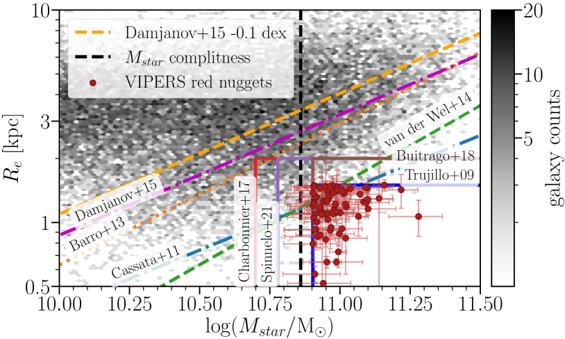
Figure 1: Stellar mass vs effective radius distribution of 36 157 galaxies within the pure sample. The magenta dash-dotted line represents the initial Damjanov et al. (2015) cut for massive compact sources, the blue solid line indicates one of the most restrictive criteria proposed by Trujillo et al. (2009), and the orange dashed line visualises the cut adopted in this work to select 6 961 UCMG candidates. The red points with error bars represent our final sample of 77 VIPERS red nuggets. The black dashed line shows the stellar mass completeness in the VIPERS catalogue. With other lines different compactness criteria are marked: blue dot-dashed line – ultracompact Cassata et al. (2011); orange dotted line – Barro et al. (2013); green dashed line – ultracompact van der Wel et al. (2014); red solid line – Charbonnier et al. (2017); brown solid line – Buitrago et al. (2018); violet solid line – Spiniello et al. (2021).

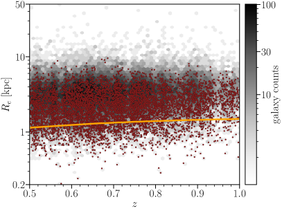
Figure 2: Distribution of effective radius as a function of redshift for 36 157 galaxies from VIPERS pure sample is shown in grey. The orange line represents the VIPERS’ seeing-detection limit. The UCMG candidates are marked with red circles.

The orange solid line in Figure 2 represents the seeing-detection limit. The CFHTLS $i$ images used by Krywult et al. (2017) have a pixel scale of 0.186^′′. The mean seeing, defined by the Full Width at Half Maximum (FWHM) of stellar sources, depends on the CFHTLS filter. According to Goranova, Y. et al. (2009) it is equal 0.64^′′ for i/iy-band. The angular size limit is transformed into physical units of $R_{e}$ as a function of redshift, which is shown as an orange solid line in Fig. 2. A vast majority of both pure sample (33 810, $\sim$93.5%), and UCMG candidates (5 673, $\sim$81%) have sizes larger than the pixel size. We decided not to remove sources lying below the seeing-detection limit by default, but in the next steps of our analysis, we verified their properties more carefully (see Sec. 4).

Table 2: Summary of initial cuts performed to select firstly pure sample, and then UCMG candidates.

Cut	Sample size
VIPERS database	91 507
$z_{flag}\in\{3,4,23,24\}$	54 252
Redshift range $0.5\leq z\leq 1$	44 145
$R_{e}$ uncertainties and relative errors $<$ 100%	36 157
UCMG candidates (based on Equation 2)	06 961

3 Stellar mass re-estimation

We decided to recalculate stellar masses of UCMG candidates as a part of the quality check. As the stellar mass is one of the two parameters which characterises compact sources, it is obligatory to take into account the goodness of the fit and uncertainties, which were not derived so far for VIPERS galaxies. For this purpose, we used the state-of-art SED fitting tool called Code Investigating GALaxy Emission (CIGALE; Boquien et al. 2019). We used CIGALE, as it models the SED of galaxies by conserving the energy balance between the dust-absorbed stellar emission and its re-emission in the IR. The capabilities of this SED fitting tool have already been verified on VIPERS observations (i.e., Rałowski et al. 2020; Vietri et al. 2021; Turner et al. 2021; Pistis et al. 2022, Figueira et al., in prep.). Previous works have estimated stellar masses, SFRs, and AGN fractions of VIPERS’ observed galaxies, and have shown consistency between each other. Moreover, we checked the stellar masses and absolute magnitudes obtained from CIGALE and Le Phare (Arnouts et al. 1999; Ilbert et al. 2006) and found homogeneous results, which suggest that our SED fitting procedure is independent on the SED fitting methodology. In this analysis, we assumed a delayed star formation history, Bruzual & Charlot (2003) single stellar population models with the initial mass function (IMF) given by Chabrier (2003), Charlot & Fall (2000) attenuation law and the dust emission models of Dale et al. (2014) to build a grid of models.

In the case of stellar mass estimation, the used attenuation curve plays a significant role (on average leading to disparities of a factor of two, Małek et al. 2018; Buat et al. 2019). For that reason we decided to test two very well know attenuation laws: modified attenuation laws of Charlot & Fall (2000), and Calzetti et al. (2000). As the VIPERS sample lacks reliable IR data we decided to use Calzetti et al. (2000) law. Here, we want to stress that the stellar mass obtained with Charlot & Fall (2000) recipe is systematically higher by $\sim$ 0.1 dex than Calzetti et al. (2000). A more detailed description can be found in the App. A. Moreover, we suspect that the amount of dust in galaxies we are looking for is rather low and therefore we do not expect to find a huge difference between both methods. Nevertheless, in our SED fitting approach, for the dust attenuation model, we used a wide range of parameters, allowing us to construct and fit templates similar to normal-star forming galaxies with a significant amount of dust. The final input parameters used in SED fitting with CIGALE are presented in Table 5. A detailed description of each module can be found in Małek et al. (2018) and Boquien et al. (2019).

CIGALE estimates the physical properties of galaxies by evaluating a generated grid of models on data to minimise the likelihood distribution. The quality of the fit is expressed by the reduced value of the $\chi^{2}$ parameter. The physical properties and their uncertainties are estimated as the likelihood-weighted means and standard deviations. The mean goodness of the fit in UCMG candidates sample, assuming input as shown in Tab.5, is $\chi^{2}\simeq 0.8$, and the mean uncertainties of stellar masses are at the level of 19%. Hereafter, every time the stellar masses of UCMG candidates is mentioned, we refer to $M_{star}$ obtained by our SED fitting.

Table 3: Report of the compactness formulae and redshift ranges of sources presented in the literature. The number of UCMG candidates according to each criterion is given in the fourth column. The last column provides sample size of UCMG candidates, which meet the compactness criterion and the mass completeness, above $\log(M_{star}/\rm{M}_{\odot})\geq 10.86$ (Davidzon et al. 2016). Two works (Cassata et al. 2013; van der Wel et al. 2014) applied two different criteria, and we refer to them as a ‘compact’ and ‘ultracompact’ for less and more restrictive, respectively.

Reference	Redshift	Formula	Number of sources	Mass complete
Damjanov et al. (2015)	0.24 - 0.66	(log($R_{e}$) + 5.74)/log(M) ¡ 0.568	4 347	1 664
Cassata et al. (2011) – compact	1.20 - 3.00	(log($R_{e}$) + 5.5)/log(M) ¡ 0.54	3 139	1 115
Barro et al. (2013)	1.40 - 3.00	log(M/$R_{e}^{1.5}$) ¿ 10.3	3 083	1 370
van der Wel et al. (2014) – compact	0.00 - 3.00	$R_{e}$/(M/1011)0.75 ¡ 2.5 kpc	1 801	0 914
Charbonnier et al. (2017)	0.20 - 0.60	log(M) ¿ 5 $\times$ 1010, $R_{e}$ ¡ 2 kpc	1 061	0 372
Spiniello et al. (2021)	0.10 - 0.50	log(M) ¿ 6 $\times$ 1010, $R_{e}$ ¡ 2 kpc	2 693	0 372
Buitrago et al. (2018)	0.02 - 0.30	log(M) ¿ 8 $\times$ 1010, $R_{e}$ ¡ 2 kpc	2 277	0 277
Cassata et al. (2011) – ultracompact	1.20 - 3.00	(log($R_{e}$) + 5.8)/log(M) ¡ 0.54	2 250	0 082
van der Wel et al. (2014) – ultracompact	0.00 - 3.00	$R_{e}$/(M/1011)0.75 ¡ 1.5 kpc	2 241	0 134
Trujillo et al. (2009)	0.00 - 0.20	log(M) ¿ 8 $\times$ 1010, $R_{e}$ ¡ 1.5 kpc	22 86	0 086

4 Final selection of red nugget sample

In this section, we present the final criteria used to select the population of VIPERS red nuggets from our sample of 6 961 UCMG candidates. In particular, we considered different definitions of compactness given by the limits in size, $R_{e}$, and stellar mass, $M_{star}$, followed by restricting the sample to red, passive galaxies based on their colours and star formation rate (hereafter SFR).

4.1 Compactness

The criterion used to select UCMGs, in particular the threshold for stellar mass and effective radius, has a great influence on the size and properties of the selected sample. Several different studies defined the class of massive compact galaxies based on various selection criteria (e.g Trujillo et al. 2009; Damjanov et al. 2015; Charbonnier et al. 2017). To make a reliable comparison with literature, we adopt different definitions following selections that other authors have used. The list of criteria applied to select massive and compact galaxies is given in Table 3. Different criteria can change the number of UCMGs by a factor of $\sim$50. In particular, using the least conservative criterion proposed by Damjanov et al. (2015), we end up with 4 347 UCMGs, while the criterion of Charbonnier et al. (2017) defined in the same redshift range, results in 1 061 galaxies. In our VIPERS red nuggets catalogue we included only sources, which meet one of the most restrictive criteria given by authors. We used criterion proposed by Trujillo et al. (2009): $M_{star}>8\times 10^{10}$ ($\log(M_{star}/\rm{M}_{\odot})\gtrsim 10.9$) and $R_{e}>1.5$ kpc, which limits the sample to only 86 objects (hereafter VIPERS UCMGs).

We performed a test, we found that if applying compactness and stellar mass completeness cuts together, the Cassata et al. (2011) criterion gives fewer sources above the stellar mass completeness threshold (82 red nuggets candidates versus 86 from Trujillo et al. (2009) criterion). However, we wanted to focus on truly compact objects, thus we used the Trujillo et al. (2009) criterion, which is very strict in the $R_{e}$. Moreover Trujillo et al. (2009) criterion is easiest to perform as it has two separates cuts for stellar mass and effective radius. I allows to control not only the compactness cuts, but also it is easy to compare with mass completeness.

The Trujillo et al. (2009) criterion was used in the literature to select UCMGs up to $z\sim 0.5$ (Tortora et al. 2016; Scognamiglio et al. 2020). Although, this work aims to select UCMGs at the intermediate redshift range ($0.5<z<1.0$), we do not expect significant changes to the selection criterion. We assume that if UCMGs survive from $z>3$ to the local Universe, $z<1$, then their main physical properties such as $R_{e}$ and $M_{star}$ do not change significantly. This implies that they evolved relatively unaltered, without mergers or influence of other galaxies. For that reason, we can use the same compactness criterion for UCMGs from $z\sim 2$ to $z\sim 0$.

According to Davidzon et al. (2016), applying a cut in stellar mass assures stellar mass completeness in the VIPERS sample up to $z=0.9$ ($\log(M_{star}/\rm{M}_{\odot})\geq 10.86$). We calculated the stellar mass threshold above which passive galaxies can be considered complete in stellar mass in the redshift range 0.9–1.0. We have found, using the Pozzetti et al. (2010) method, which was also used in Davidzon et al. (2016), the stellar mass threshold at the limit of ${\log}(M_{star}/\rm{M}_{\odot})=11.03$. However, taking into account the low number of known red nuggets in the intermediate redshift, we decided to enlarge our analysis using the same cut in mass, ${\log}(M_{star}/\rm{M}_{\odot})=10.86$, up to redshift 1, even with possible incompleteness bias for the most distant sources. In this step of our selection, we also took into account the seeing-size limit. As we mentioned before, the majority of UCMG candidates (5 673, $\sim$81%) are larger than the size of pixel, but $\sim$73% (63 galaxies) of VIPERS UCMGs have sizes measurements below seeing-defined limit (see Fig. 2). After visual inspection of a sample of 86 VIPERS UCMGs we found that images of all selected galaxies show compact and elliptical galaxy profiles with no signs of spiral arms or other morphological disturbances, and we decided to use all of them in our further analysis.

4.2 Passiveness

To select red and passive galaxies, we performed multistage selection based on the colours, emission lines, and final visual inspection.

4.2.1 NUVrK diagram

The primary criterion to select red sources used in our work is their position on the colour–colour diagram. In our work, we used the NUVrK diagram, which is a tool to select a complete and pure sample of red passive galaxies, as this combination of colours allows to break dust-SFR degeneracy (Arnouts et al. 2013). It is widely used by the VIPERS team, see for example: Fritz et al. (2014), Davidzon et al. (2016), Moutard et al. (2016b, 2018), Gargiulo et al. (2017), Siudek et al. (2018a, b), Turner et al. (2021). The NUVrK diagram is shown in Fig 3. All points (red and green) show the positions of 86 VIPERS UCMGs. The orange line shows the boundary between red and blue galaxies derived by Moutard et al. (2016b) obtained for the VIPERS survey. As one can clearly see, seven galaxies lie below the limit, even while taking into account uncertainties. Those seven galaxies are marked with green crosses and have been removed from our sample for the next steps (79 objects left).

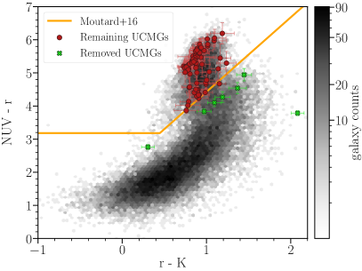
Figure 3: NUVrK diagram. The distribution of 36 157 galaxies (pure sample) is shown in the background. The orange line shows the limit for red galaxies adapted from Moutard et al. (2016b). The red and the green points represent our VIPERS UCMGs sample. Sources marked with green crosses are considered as blue (active) and have been removed from our sample.

4.2.2 Visual inspection of VIPERS spectra

To verify the passiveness of the selected 79 red UCMGs, we checked their spectra obtained by VIPERS. We performed a detailed visual inspection of every object in the sample, searching for characteristic features which indicate star-forming activity, such as oxygen emission lines (Kennicutt 1992), lack of CaII absorption lines or low Balmer break value (hereafter D4000; Bruzual A. 1983; Haines et al. 2017). Figure 4 shows examples of possibly active (top panel) and passive (bottom panel) galaxies in our sample of VIPERS UCMGs. The major differences are: the presence of a strong O[II] emission line, the lack of the CaII absorption lines and a weak D4000 in the active spectrum (top panel). In our sample of 79 UCMGs, we found two objects which likely show active galaxy features. At this point, we left 77 UCMGs which we consider as red nugget candidates.

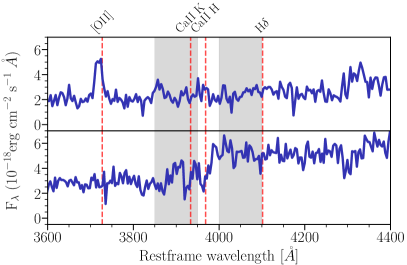
Figure 4: Exemplary spectra of galaxies. The upper panel shows a possible star-forming galaxy while the bottom panel shows a likely passive galaxy. With red dashed lines we marked from left: [OII] emision line(3727.5 Å), calcium K (3933.7 Å), calcium H (3968.5 Å), H$\delta$ (4101.7 Å). The grey shadings correspond to regions used for D4000 calculation (Balogh et al. 1999)

4.2.3 Sanity check

As a final sanity check of passiveness of the selected sample of 77 passive UCMGs, we examined the stellar mass – SFR relation, known also as the main sequence (hereafter MS). Figure 5 shows the SFR as a function of the stellar mass of our 6 961 galaxies which belong to the UCMG candidates. Red circles and pink triangles represent the sample of 77 VIPERS red nuggets candidates, and green crosses show the galaxies, which have been removed from our sample in previous steps. The orange solid line shows the limit for passive objects used by Salim et al. (2018), defined as specific SFR (SFR over stellar mass) equal to $10^{-11}$ $\rm{yr}^{-1}$. The blue solid line shows the MS of star-forming galaxies derived by Schreiber et al. (2015). Here we plotted the MS at redshift $z\simeq 0.83$, which is the median redshift, of the sample of 86 VIPERS UCMGs. In addition to that, the blue shaded region shows the range where $\log(\rm{SFR}/\rm{SFR}_{\rm{MS}})<\log(4)\sim 0.6\rm{\leavevmode\nobreak\ dex}$. It is a widely used limit to select both starbursting and passive galaxies from the main sequence relation (eg: Elbaz et al. 2018; Buat et al. 2019; Donevski et al. 2020). We found only three sources which were not removed in previous steps above the Salim et al. (2018) passiveness limit, but considering uncertainties in estimating both the SFR and stellar mass, as well the passive nature of their spectra, we decided to keep them in the sample. Taking into account the uncertainties, none of the 77 UCMGs is considered a MS galaxy. For those reasons, we decided to not remove any additional sources. Finally, we established a sample of confirmed VIPERS red nuggets containing 77 sources.

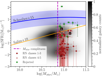
Figure 5: Relation of SFR vs stellar mass. In the smoothed background the sample of 6 961 UCMG candidates is shown. Points represent our red and green 86 UCMGs. Red circles and pink triangles indicate VIPERS red nuggets (RN), while green crosses correspond to the UCMGs, which we considered as active. The orange line shows the limit for passive galaxies (Salim et al. 2018). The blue line shows the main sequence of galaxies according to Schreiber et al. (2015). The magenta dashed line shows the mass completeness at redshift $z=$ 0.9 for passive galaxies equal to $\log(M_{star}/M_{\odot})\sim 10.86$ according to Davidzon et al. (2016). The three sources with relative errors higher than 45% are marked with black squares.

5 Final catalogue of VIPERS red nuggets - properties

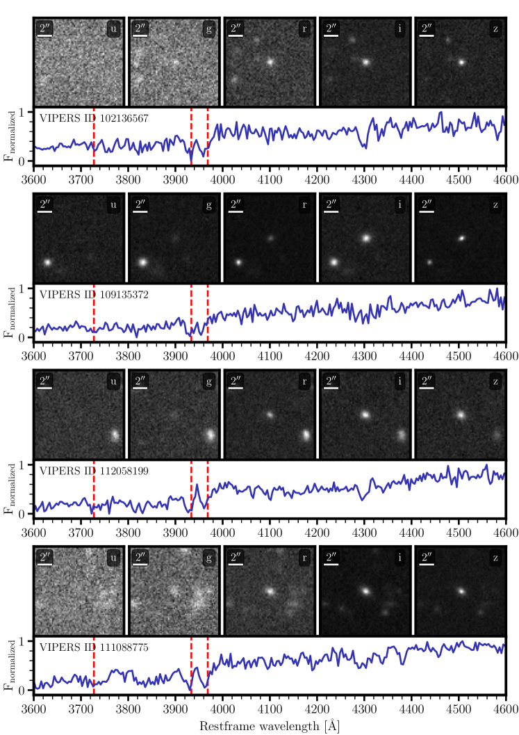
Figure 10: Examples of red nuggets in our catalogue. For every galaxy we show images in the u, g, r, i, and z bands from the CFHT survey, and normalized spectra with wavelength of oxygen [OII] emission line (3727.5 Å), calcium CaII K (3933.7 Å) and H (3968.5 Å) absorption lines marked.

In Table 3 we listed the number of selected UCMGs corresponding to different compactness definitions from the literature. Within the VIPERS red nuggets catalogue we only considered the sample obtained using one of the most restrictive criteria for compactness, with $M_{star}>8\times 10^{10}$ M_⊙ and $R_{e}<1.5$ kpc (Trujillo et al. 2009), resulting in 86 UCMGs. We then selected the 77 VIPERS red nuggets based on the NUVrK criterion, visual inspection of their spectra and additional sanity checks (see Sec. 4.2). Figure 10 shows four examples of selected red nuggets. We present not only the images in the u, g, r, i, and z bands from the CFHT survey, but also the normalized spectra with marked oxygen [OII] (3727.5 Å), calcium CaII K (3933.7 Å) and CaII H (3968.5 Å) lines. The VIPERS red nuggets catalogue is publicly available and reported in Appendix C. In the catalogue, we list VIPERS IDs and positions in the sky, as well as all important parameters used in analysis such as: redshifts, effective radii, stellar masses and colours.

One characteristic that sets this study of red nuggets apart from other works is the unique redshift range over a wide-field systematic survey. In addition to that, our sample is already spectroscopically confirmed, which is an improvement in comparison with studies based only on photometry. This means that we present the largest catalogue of spectroscopically identified red nuggets beyond the local Universe. In comparison, there is only 14 confirmed quiescent compact galaxies within the Baryon Oscillation Spectroscopic Survey (BOSS) at redshift $0.2<z<0.6$ (Damjanov et al. 2014) and about $\sim$20 found by Charbonnier et al. (2017) in the CFHT equatorial SDSS Stripe 82, also at redshift range $0.2<z<0.6$.

Within our final catalogue of red nuggets 96% of all galaxies (74 sources) have relative errors of $R_{e}$ lower than 45%. The remaining three red nuggets with the relative errors of $R_{e}$ equal to 99%, 62% and 61% included in our sample are highlighted in Table C with underlined IDs and $R_{e}$ values, and in Fig. 5 with black squares.

5.1 Comparison with VIPERS’ results of unsupervised classification

We performed a cross-match of our 77 red nuggets with detailed classification done by Siudek et al. (2018b). In this paper, the authors classified 52 114 VIPERS galaxies with the highest confidence ($>90\%$) of redshift measurements into 12 classes using the unsupervised machine learning algorithm, Fisher Expectation-Maximization (FEM; Bouveyron & Brunet 2012). All subclasses found by Siudek et al. (2018b) mirror substructures in the bimodal colour distribution of galaxies, distinguishing subpopulations of passive (red), intermediate (green) and active (blue) galaxies and an additional class of broad-line AGNs. In the following section, the definition of the red, green and blue galaxy populations relies on FEM classification:

• red (subclasses 1–3),

• green (subclasses 4–6),

• blue (subclasses 7–11).

The reliability of those three classes was checked in Siudek et al. (2018b) via colour-colour method, spectral features like emission line distributions and the spectral continuum, and morphological parameters like Sérsic index, stellar mass and SFR. We refer to Siudek et al. (2018a, b, 2022) for a detailed description of the VIPERS classification. In this paper, we verify if VIPERS’ red nuggets are preferably found in one of the red subclasses.

Our sample of 77 VIPERS red nuggets contains 72 red-class galaxies (subclasses 1–3) marked in Fig. 5 as red circles, and five galaxies which belong to subclasses 4–5, green classes, represented in Fig. 5 with pink triangles. All five green galaxies lie closer to the main sequence relation than the rest of the red nuggets, which additionally supports the reliability of FEM classification from Siudek et al. (2018b). A histogram of red nuggets’ classes is also presented in Fig. 7. We did not find galaxies from the blue classes which supports our classification of passive, massive compact objects. Almost 65% (49 out of 77) red nuggets are found in the subclass 1, which gathers massive, and small red galaxies (see Tab. 1 and Sec. 5.3 in Siudek et al. 2022) This confirms the usefulness of applying unsupervised machine-learning algorithms to automatically find ‘peculiar’galaxy subclasses (Siudek et al. 2018a, b, 2022).

5.2 The D4000 distribution of intermediate-$z$ red nuggets

The strength of the 4000 Å spectral break (hereafter D4000, defined as in Balogh et al. 1999) is one of the main and direct characteristics of the star formation history of galaxies. Its correlation with young and evolved stellar populations makes this spectral index suitable as a passiveness indicator (i.e. Kauffmann et al. 2003a, b; Siudek et al. 2017; Haines et al. 2017).

Figure 6 shows D4000 – $z$ (top panel) and $M_{star}$ – $z$ (bottom panel) relations, where grey points represent 77 red nuggets, the red squares are median values calculated for four redshift bins defined for similar number of objects (see Tab. 4). The red lines show the linear fit to the median values. In addition to that, the orange dashed line indicates D4000 = 1.55 – the passiveness boundary found by Kauffmann et al. (2003a) for the local Universe based on the SDSS survey. Taking into account uncertainties of D4000 measurements, six galaxies lie below the Kauffmann et al. (2003a) limit. Two of those galaxies have $z\sim 0.73$, while four are located at the end of our redshift range, at $z>0.85$, where we can expect to see a younger population than in the local Universe.

Considering the median values in redshift bins, there is no significant D4000–$z$ dependence for the presented sample, and the median value of D4000 for red nuggets in the redshift range 0.5-1.0 stays constant at the level 1.66$\pm$0.05 indicating passiveness of the sample. The bottom panel of Fig. 6 shows the $M_{star}$–$z$ relation for the sample of 77 red nuggets. We found no clear dependence of the stellar mass on redshift. However, the highest redshift bin may be biased by non negligible incompleteness.

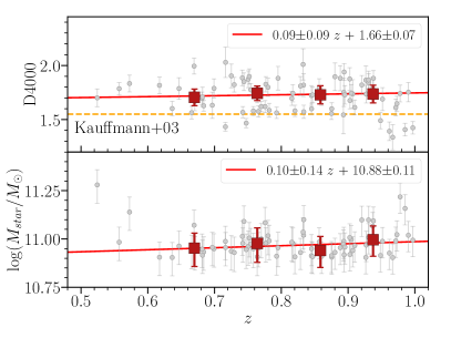
Figure 6: Relation of D4000 vs $z$ in the top panel and $M_{star}$ vs $z$ in the bottom panel. Grey points represent 77 red nuggets and the red squares represent the median value in every redshift bin (see Tab. 4), and the red line is the best linear fit. The dashed orange line represents D4000 equals 1.55, which is considered a passiveness limit derived by Kauffmann et al. (2003a) in the local Universe.

6 Discussion and results

6.1 Influence of compactness criteria on sample size

All compactness criteria found in literature are functions of $R_{e}$ and $M_{star}$. The discrepancy of those criteria is shown in Tab. 3. Unfortunately, we can not compare samples sizes of UCMGs found by different criteria, as not all of them are mass complete. For this reason, we additionally limit the criteria by cutting all galaxies with stellar masses below the completeness limit. In the VIPERS survey, the number of sources considered as compact and complete in stellar mass found here varies between 1 664, while using the Damjanov et al. (2015) criterion, and 82 with Cassata et al. (2011) ultracompact criterion. We thus see that the choice of compactness criterion can influence the sample size by up to a factor of $\sim$20.

6.2 Evolution of number densities

In order to derive number densities, we divided all red nuggets into four redshift bins containing a roughly equal number of galaxies per bin: 0.50–0.72, 0.72–0.82, 0.82–0.9 and 0.90–1.00 (see Table 4). Taking into account that our sources are not evenly distributed in redshift (see Fig. 7) our bins are not uniform. We then calculated weighted number of sources based on TSR and SSR of the parent sample:

$$\rm{N_{w}}=\sum_{i}^{\rm{N}}(\rm{TSR}_{i}\cdot\rm{SSR}_{i})^{-1},$$ (3)

(for details see Garilli et al. 2014). Finally, we normalized our bins to the comoving volume corresponding to the VIPERS observed area and calculated the number density per cubic comoving Mpc. The results are presented in Table 4 and in Figure 8.

Table 4: Overview of the four redshift bins and the summary of all four bins. The second column shows the number of sources in each bin, and the third one presents the weighted number of sources, which takes into account the TSR and SSR. In the last column, we show the number density per comoving cubic Mpc.

Redshift range	N	Nw	Number density [$\rm{Mpc}^{-3}$]
$0.50\leq z\leq 0.72$	16	39.25	$4.74\times 10^{-6}$
$0.72<z\leq 0.82$	21	56.75	$1.14\times 10^{-5}$
$0.82<z\leq 0.90$	18	55.64	$1.23\times 10^{-5}$
$0.90<z\leq 1.00$	22	61.05	$9.82\times 10^{-6}$
$0.50\leq z\leq 1.00$	77	212.69	$8.86\times 10^{-6}$

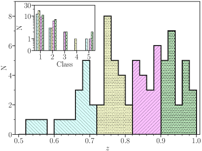
Figure 7: Distribution of VIPERS red nuggets in redshift (big histogram) and in FEM classes (smaller one). Different colours correspond to our bins.

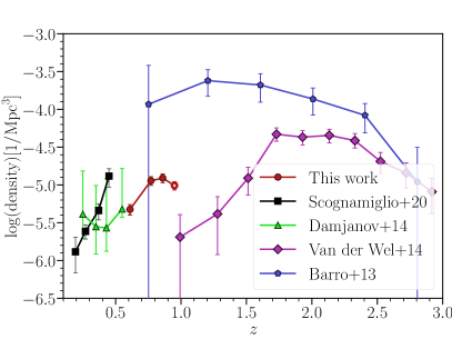
Figure 8: Number density per comoving cubic Mpc vs redshift. The red points show results from this work, the green ones show the quiescent compact galaxies found by Damjanov et al. (2014), the black ones show the compact galaxies found by Scognamiglio et al. (2020), the violet ones show ultracompact ETGs analysed by van der Wel et al. (2014) and the blue ones present the quiescent compact galaxies found by Barro et al. (2013).

Figure 8 shows number densities (see Tab. 4) as a function of redshift. Number densities of VIPERS red nuggets calculated in the first three redshift bins are marked with the full redcircles, while the results from the redshift bin 0.9–1.0 which can be biased by the mass incompleteness, is shown as a red open circle. We stressed that due to the mass incompleteness presented number density for this redshift bin should be considered as a lower limit. Presented uncertainties of the number counts take into account fluctuations due to the Poisson noise.

We compared our results with the number densities of quiescent compact galaxies found by Damjanov et al. (2014) in the Baryon Oscillation Spectroscopic Survey, which are marked with green triangles. In addition to that, we also plotted the number densities of ultracompact massive galaxies found in the Kilo Degree Survey by Scognamiglio et al. (2020). Those results are shown as black squares. As we do not expect to find in this sample a statistically significant number of star-forming massive compact objects (for example in our initial sample of 86 UCMGs only $\sim$10% were considered as not passive), it is reasonable to compare those two groups. At higher redshifts, we present passive ultracompact galaxies found in the CANDELS field by van der Wel et al. (2014) marked with purple diamonds (found with the ultracompact criterion, see Tab. 3). Moreover, we also show the quiescent compact sources found in the GOODS-S and UDS fields of CANDELS by Barro et al. (2013) with blue pentagons. None of the high-redshift studies provide explicit number densities, and an online tool was used to extract their corresponding values directly from plots.

Figure 8 shows that our results are in overall agreement with the lower-redshift studies, to within an order of magnitude. However, the trends found by Scognamiglio et al. (2020) and Damjanov et al. (2014) are slightly different, as those samples were selected using a slightly different approach: (1) Damjanov et al. (2014) selected objects with effective radius smaller than $R_{e}<2$ kpc (in our work $R_{e}<1.5$ kpc) while the cut on stellar mass is the same as the one used in this work ($M_{star}<8\times 10^{10}$). Moreover, the resulting numbers from Damjanov et al. (2014) are considered as the lower limits for number density due to sample incompleteness. (2) Scognamiglio et al. (2020) performed a statistical correction, taking into account false positives and false negatives. For the first three bins (redshift lower than 0.4), this correction does not change the number density values significantly (uncorrected results are still inside error bars). However, the uncorrected value of the last bin is lower by around twice the error value. In Figure 8 we show only corrected number densities. The criteria used for selecting compact sources are exactly the same as the ones we used ($M_{star}<8\times 10^{10}$ and $R_{e}<1.5$ kpc). However, the authors do not discuss the subject of passiveness.

To summarize, Figure 8 shows that, our results match the ones presented in Damjanov et al. (2014). Similarly, the results obtained by Scognamiglio et al. (2020), except the number density at $z\sim$0.45, match smoothly with our results. However, as mentioned before, the uncorrected value of the last point is $\sim$0.3 dex lower.

On the other hand, at high-redshifts, the differences are significant. However, both van der Wel et al. (2014) and Barro et al. (2013) used radically different, less conservative, compactness criteria from those used in this work. In addition to that, we cannot straightforwardly compare the number of VIPERS UCMGs selected using the same criteria due to the mass completeness. For this reason, here only the mass complete sample sizes are discussed (see Tab. 3). Considering only mass complete samples of UCMGs, we find that the Trujillo et al. (2009) criterion (our fiducial choice throughout this work) yields roughly 1.5 and 14 times fewer compact sources than the Barro et al. (2013) and van der Wel et al. (2014) criteria, respectively. Comparing the number density presented by Barro et al. (2013) at $z\sim$0.75 to the number density of the VIPERS red nuggets at $z\sim$0.63, we find the former to be $\sim$20 times larger. As the ratio of number densities is similar to our inferred ratio of the number of sources found with the different criteria, we conclude that our results are consistent with those of Barro et al. (2013). Nevertheless, the number density of VIPERS red nuggets at $z\sim$0.95 is roughly 5 times larger than the number density reported by van der Wel et al. (2014) at z$\sim$1. The cause of this disagreement is unclear.

7 Summary

We have shown that the sample size of UCMGs in the uniform spectroscopic VIPERS survey is strongly dependent on the compactness criterion, and comparing the different criteria is not straightforward. Our catalogue of 77 VIPERS red nuggets significantly increases the number of known sources. The brand new catalogue of red nuggets presented here is a solid framework for future studies. Very restricted selection cut (based on $R_{e}$, $M_{star}$ and passiveness indicators) provides a pure sample of intermediate-redshift red nuggets. The evolution of the number density of red nuggets and relics over cosmic time is still an open issue. The results presented here provide a next step to understanding the evolution of red nuggets. We were able to trace the number densities of red nuggets with a comparable statistical significance to the one found at lower redshifts (Charbonnier et al. 2017; Scognamiglio et al. 2020). The detailed analysis of their physical properties to reveal their nature is left for future work and their environmental properties are discussed in Siudek et al. in prep.

Appendix A Attenuation

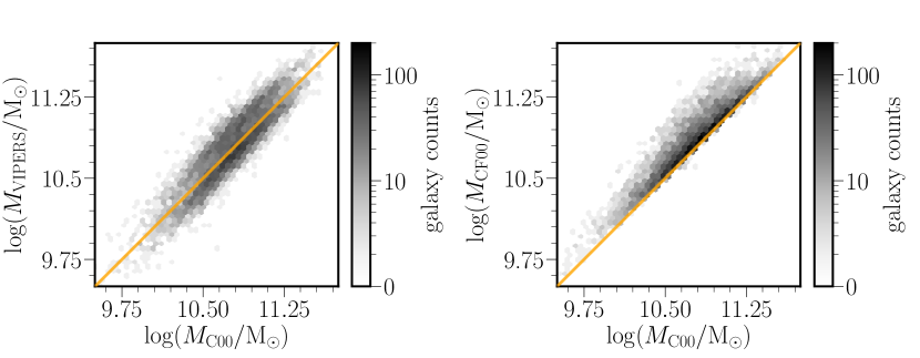
Figure 9: The left panel shows comparison of stellar masses calculated via CIGALE with Calzetti et al. (2000) attenuation law, $M_{\rm{C00}}$, with those calculated by the VIPERS team using Le Phare tool (Arnouts et al. 1999; Ilbert et al. 2006), $M_{\rm VIPERS}$ for 36 157 galaxies in the pure sample. The right panel shows comparison of stellar masses calculated with CIGALE using Calzetti et al. (2000) and Charlot & Fall (2000) $M_{\rm CF00}$ attenuation laws for the same pure sample of galaxies. On both plots one to one relation was marked with an orange line.

Table 5: Input parameters used in SED fitting with CIGALE.

Parameter	Values
Delayed star formation history
e-folding time of the main stellar population model (Myr)	100, 300, 500, 1500
Age of the main stellar population	300, 500, 800, 1000, 2500,
in the galaxy (Myr)	3500, 4500, 6000, 7000
e-folding time of the late starburst population model (Myr)	10000
Age of the late burst (Myr)	10
Mass fraction of the late burst population	0
Normalise the SFH to produce one solar mass	True
Stellar population synthesis Bruzual & Charlot (2003)
Initial mass function	Chabrier (2003)
Metalicity	0.02
Age of the separation between the young and the old star populations (Myr)	10
Dust emission Dale et al.2014
AGN fraction	0
$\alpha$ slope	2.0
Dust attenuation Charlot & Fall (2000)
V-band attenuation in the interstellar medium	0.0, 0.05, 0.1, 0.2, 0.4, 0.75,
	1.0, 1.5, 1.75, 2.0, 2.2, 2.5, 3.0
$\mu$	0.8
Power law slope of the attenuation in the ISM	-0.7
Power law slope of the attenuation in the birth clouds	-0.7
Dust attenuation Calzetti et al. (2000)
E(B-V)l	0.0,0.05, 0.1, 0.2, 0.3, 0.4, 0.5,
	0.6, 0.7, 0.8,0.9, 1.0 ,1.3, 1.5
E_BV factor	0.44
Central wavelength of the UV bump in nm	217.5
Width (FWHM) of the UV bump in nm	35.0
Amplitude of the UV bump	0
Slope delta of the power law modifying the attenuation curve	0
Extinction law to use for attenuating the emission lines flux	Milky Way
Ratio A_V / E(B-V)	3.1

Figure 9 shows that stellar masses estimated with the Calzetti attenuation law (Calzetti et al. 2000) are much closer to the ones originally estimated using the Le Phare SED fitting tool (Arnouts et al. 1999; Ilbert et al. 2006) by the VIPERS team. The mean scatter between our results obtained with the Calzetti attenuation law and the VIPERS stellar masses is less than 0.02 dex. The median difference obtained with both attenuation laws is $\sim$0.1 dex. The Calzetti model is simpler and has fewer degrees of freedom than the double power law model of Charlot & Fall (2000), which assumes separate power laws for the birth cloud and one for the interstellar medium. As we lack reliable IR data, this is an advantage in this case. We therefore decided to use in our analysis results obtained with Calzetti et al. (2000) law.

Appendix B Examples of VIPERS’ red nuggets

Appendix C Catalogue of red nuggets

Table 6: Catalogue of VIPERS red nuggets. We present the main physical properties used in our analysis. The first column contains VIERS ID, the next two show the sky position, the third one shows redshift, Ra, Dec, $z$. The next two columns contain physical properties like circularised half-light radii, stellar mass respectively. The last two columns show the colours used for passiveness checking: NUV - r and r - K. Three VIPERS IDs, together with their R_e values, are underlined, as their relative errors of $R_{e}$ are higher than 45%.

VIPERS ID	Ra [deg]	Dec [deg]	$z$	$R_{e}$ [kpc]	$\log(M_{star})$ [$\rm{M}_{\odot}$]	NUV - r	r - K
101131036	130.5258639	-5.9354478	0.997	0.73 $\pm$ 0.11	10.99 ${}^{+0.03}_{-0.03}$	4.41 $\pm$ 0.09	0.99 $\pm$ 0.09
102136567	131.5245661	-5.8885126	0.927	1.19 $\pm$ 0.51	10.90 ${}^{+0.08}_{-0.09}$	5.39 $\pm$ 0.21	0.85 $\pm$ 0.09
102164621	131.5018244	-5.7478308	0.845	1.10 $\pm$ 0.13	10.91 ${}^{+0.07}_{-0.09}$	5.36 $\pm$ 0.16	0.83 $\pm$ 0.09
103137838	132.7348014	-5.9634442	0.750	1.31 $\pm$ 0.11	10.96 ${}^{+0.08}_{-0.10}$	5.26 $\pm$ 0.38	0.95 $\pm$ 0.10
104169502	133.3173687	-5.9113035	0.766	0.65 $\pm$ 0.04	10.95 ${}^{+0.05}_{-0.06}$	5.21 $\pm$ 0.25	0.88 $\pm$ 0.11
104243009	133.5006282	-5.6283503	0.742	1.37 $\pm$ 0.13	11.01 ${}^{+0.07}_{-0.08}$	6.03 $\pm$ 0.16	1.01 $\pm$ 0.10
105149946	134.9739041	-5.9108378	0.777	1.15 $\pm$ 0.07	10.98 ${}^{+0.07}_{-0.09}$	5.50 $\pm$ 0.18	0.84 $\pm$ 0.08
106178573	135.4706881	-5.7853115	0.776	1.25 $\pm$ 0.06	11.08 ${}^{+0.03}_{-0.03}$	5.19 $\pm$ 0.08	0.74 $\pm$ 0.08
107109094	136.6137710	-5.9471244	0.820	1.24 $\pm$ 0.08	10.91 ${}^{+0.04}_{-0.05}$	4.23 $\pm$ 0.11	0.91 $\pm$ 0.11
107115227	136.5739924	-5.9120644	0.978	1.42 $\pm$ 0.26	11.22 ${}^{+0.06}_{-0.07}$	5.33 $\pm$ 0.15	0.83 $\pm$ 0.08
107156787	136.0857272	-5.6749818	0.684	1.14 $\pm$ 0.09	10.93 ${}^{+0.05}_{-0.06}$	4.69 $\pm$ 0.25	0.89 $\pm$ 0.08
109135372	137.9142200	-5.8984831	0.833	0.84 $\pm$ 0.27	11.02 ${}^{+0.08}_{-0.09}$	5.56 $\pm$ 0.23	0.90 $\pm$ 0.09
109179636	138.3647960	-5.6751634	0.524	1.07 $\pm$ 0.21	11.28 ${}^{+0.08}_{-0.11}$	5.81 $\pm$ 0.17	1.01 $\pm$ 0.08
110144150	130.3309573	-4.9606058	0.764	1.22 $\pm$ 0.11	10.91 ${}^{+0.08}_{-0.10}$	5.66 $\pm$ 0.21	0.88 $\pm$ 0.08
111088775	131.5152978	-5.1940591	0.817	1.47 $\pm$ 0.14	10.98 ${}^{+0.08}_{-0.09}$	5.58 $\pm$ 0.20	0.88 $\pm$ 0.08
111091579	131.4664203	-5.1807426	0.666	1.27 $\pm$ 0.04	10.94 ${}^{+0.06}_{-0.07}$	5.26 $\pm$ 0.13	0.79 $\pm$ 0.08
111126369	131.2330626	-5.0174692	0.857	1.22 $\pm$ 0.11	10.98 ${}^{+0.08}_{-0.10}$	5.52 $\pm$ 0.20	0.87 $\pm$ 0.08
112058199	132.8933163	-5.3494238	0.920	1.46 $\pm$ 0.17	11.10 ${}^{+0.08}_{-0.10}$	5.45 $\pm$ 0.18	0.87 $\pm$ 0.08
112117953	132.8196331	-5.0724753	0.910	0.92 $\pm$ 0.16	10.97 ${}^{+0.02}_{-0.03}$	5.20 $\pm$ 0.09	0.73 $\pm$ 0.08
112184594	132.7301990	-4.7586513	0.752	1.44 $\pm$ 0.12	11.00 ${}^{+0.08}_{-0.10}$	5.78 $\pm$ 0.18	0.92 $\pm$ 0.08
112195565	132.1520740	-4.7060957	0.669	1.36 $\pm$ 0.08	11.07 ${}^{+0.08}_{-0.10}$	5.86 $\pm$ 0.28	1.02 $\pm$ 0.09
114054377	134.8674224	-5.3974010	0.907	0.52 $\pm$ 0.01	10.94 ${}^{+0.10}_{-0.13}$	5.12 $\pm$ 0.36	1.14 $\pm$ 0.09
114188387	134.9725993	-4.8450140	0.905	0.88 $\pm$ 0.11	11.00 ${}^{+0.05}_{-0.06}$	5.33 $\pm$ 0.18	0.84 $\pm$ 0.08
115099121	135.3476297	-5.1404602	0.902	0.93 $\pm$ 0.21	11.01 ${}^{+0.07}_{-0.09}$	5.69 $\pm$ 0.19	0.93 $\pm$ 0.08
115108461	135.6193505	-5.0970254	0.833	1.44 $\pm$ 0.19	11.04 ${}^{+0.07}_{-0.09}$	5.70 $\pm$ 0.19	0.92 $\pm$ 0.08
117178615	137.5623537	-4.7490847	0.938	1.24 $\pm$ 0.18	11.09 ${}^{+0.08}_{-0.10}$	5.47 $\pm$ 0.21	0.94 $\pm$ 0.15
118035134	138.4941872	-5.4508176	0.948	0.93 $\pm$ 0.18	10.91 ${}^{+0.09}_{-0.11}$	4.34 $\pm$ 0.11	0.91 $\pm$ 0.11
118051171	138.6463163	-5.3644373	0.725	1.09 $\pm$ 0.68	10.94 ${}^{+0.09}_{-0.11}$	5.74 $\pm$ 0.20	0.91 $\pm$ 0.10
118052178	138.5611866	-5.3593346	0.937	1.07 $\pm$ 0.20	11.07 ${}^{+0.03}_{-0.04}$	5.22 $\pm$ 0.09	0.78 $\pm$ 0.08
118054089	138.7315875	-5.3489438	0.782	1.42 $\pm$ 0.15	10.99 ${}^{+0.11}_{-0.15}$	5.49 $\pm$ 0.20	0.89 $\pm$ 0.23
118058527	138.6383557	-5.3264219	0.742	1.38 $\pm$ 0.08	10.98 ${}^{+0.04}_{-0.04}$	5.18 $\pm$ 0.16	0.75 $\pm$ 0.08
118058570	138.7665364	-5.3267823	0.860	0.92 $\pm$ 0.14	10.91 ${}^{+0.09}_{-0.11}$	5.45 $\pm$ 0.17	0.86 $\pm$ 0.12
119108256	130.9170954	-4.1747378	0.816	1.11 $\pm$ 0.10	10.98 ${}^{+0.08}_{-0.10}$	5.42 $\pm$ 0.17	0.84 $\pm$ 0.11
120083762	131.8664909	-4.3497990	0.962	1.15 $\pm$ 0.15	10.93 ${}^{+0.08}_{-0.10}$	4.70 $\pm$ 0.23	0.99 $\pm$ 0.11
121065375	133.0372818	-4.3898337	0.967	0.79 $\pm$ 0.00	10.90 ${}^{+0.08}_{-0.10}$	4.49 $\pm$ 0.22	0.90 $\pm$ 0.09
121066765	132.1371147	-4.3834791	0.973	1.18 $\pm$ 0.18	11.02 ${}^{+0.04}_{-0.05}$	5.13 $\pm$ 0.20	0.79 $\pm$ 0.08
121089481	132.1151895	-4.2845186	0.780	1.39 $\pm$ 0.12	11.02 ${}^{+0.09}_{-0.11}$	5.30 $\pm$ 0.35	1.24 $\pm$ 0.12
122030630	133.7481148	-4.5429696	0.681	1.48 $\pm$ 0.07	10.95 ${}^{+0.08}_{-0.10}$	5.66 $\pm$ 0.26	0.87 $\pm$ 0.08
122057921	133.5865511	-4.4072717	0.699	1.25 $\pm$ 0.16	10.95 ${}^{+0.08}_{-0.10}$	5.77 $\pm$ 0.27	0.93 $\pm$ 0.10
123089330	134.4349917	-4.2838982	0.730	1.45 $\pm$ 0.01	10.93 ${}^{+0.07}_{-0.08}$	5.30 $\pm$ 0.37	0.88 $\pm$ 0.08
124039182	135.4891458	-4.5125297	0.834	1.16 $\pm$ 0.08	11.10 ${}^{+0.10}_{-0.13}$	4.30 $\pm$ 0.11	0.88 $\pm$ 0.08
124039429	135.1412790	-4.5114185	0.847	1.49 $\pm$ 0.11	10.91 ${}^{+0.03}_{-0.03}$	4.67 $\pm$ 0.13	1.15 $\pm$ 0.08
124070857	135.6400158	-4.3651440	0.894	1.47 $\pm$ 0.19	10.99 ${}^{+0.06}_{-0.07}$	5.15 $\pm$ 0.29	0.88 $\pm$ 0.08
127044375	138.3579640	-4.4846978	0.971	1.43 $\pm$ 0.33	10.99 ${}^{+0.06}_{-0.07}$	4.97 $\pm$ 0.32	0.80 $\pm$ 0.09
401010173	330.7162868	-0.8647405	0.758	1.09 $\pm$ 1.08	10.95 ${}^{+0.05}_{-0.06}$	3.86 $\pm$ 0.09	0.76 $\pm$ 0.14
401031898	330.7988766	-0.9561888	0.697	1.04 $\pm$ 0.11	10.96 ${}^{+0.08}_{-0.09}$	6.19 $\pm$ 0.32	1.19 $\pm$ 0.14
401174682	330.5012232	-1.5673446	0.670	1.09 $\pm$ 0.08	10.93 ${}^{+0.08}_{-0.10}$	5.74 $\pm$ 0.19	0.89 $\pm$ 0.08
401213761	330.5577447	-1.7365884	0.845	0.83 $\pm$ 0.06	10.95 ${}^{+0.03}_{-0.04}$	5.15 $\pm$ 0.20	0.74 $\pm$ 0.08
402034655	331.5967332	-0.9564622	0.985	1.50 $\pm$ 0.09	11.16 ${}^{+0.04}_{-0.04}$	4.13 $\pm$ 0.08	0.79 $\pm$ 0.10
402071577	331.7504873	-1.1141104	0.557	1.22 $\pm$ 0.04	10.98 ${}^{+0.05}_{-0.06}$	5.27 $\pm$ 0.13	0.80 $\pm$ 0.08
402075551	331.1296719	-1.1303454	0.876	1.05 $\pm$ 0.10	10.91 ${}^{+0.08}_{-0.09}$	4.02 $\pm$ 0.11	0.78 $\pm$ 0.14
402165870	331.2811478	-1.4969730	0.990	1.22 $\pm$ 0.00	11.02 ${}^{+0.07}_{-0.08}$	4.78 $\pm$ 0.25	1.00 $\pm$ 0.12
402173836	331.3283545	-1.5284091	0.770	1.11 $\pm$ 0.06	11.00 ${}^{+0.09}_{-0.12}$	4.47 $\pm$ 0.21	0.89 $\pm$ 0.11
403027664	332.5970905	-0.9475146	0.682	1.32 $\pm$ 0.08	10.92 ${}^{+0.08}_{-0.11}$	5.73 $\pm$ 0.29	0.92 $\pm$ 0.09
403033676	332.7095288	-0.9741027	0.744	1.46 $\pm$ 0.08	11.09 ${}^{+0.10}_{-0.12}$	5.45 $\pm$ 0.44	1.16 $\pm$ 0.13
403037148	332.3363850	-0.9906283	0.894	1.01 $\pm$ 0.10	10.92 ${}^{+0.04}_{-0.05}$	5.17 $\pm$ 0.17	0.76 $\pm$ 0.08
403054648	332.3993110	-1.0743524	0.893	1.50 $\pm$ 0.16	10.97 ${}^{+0.08}_{-0.10}$	5.59 $\pm$ 0.28	0.92 $\pm$ 0.12
403058809	332.3622401	-1.0945229	0.888	1.41 $\pm$ 0.15	10.95 ${}^{+0.08}_{-0.10}$	5.61 $\pm$ 0.25	0.92 $\pm$ 0.12
403081598	332.3105808	-1.1951127	0.903	0.86 $\pm$ 0.10	10.92 ${}^{+0.09}_{-0.12}$	4.41 $\pm$ 0.18	0.89 $\pm$ 0.10
403086972	332.6793812	-1.2183092	0.716	0.65 $\pm$ 0.03	10.99 ${}^{+0.09}_{-0.12}$	4.41 $\pm$ 0.24	0.85 $\pm$ 0.09
403099223	332.4299073	-1.2729087	0.747	1.47 $\pm$ 0.10	10.95 ${}^{+0.09}_{-0.11}$	4.56 $\pm$ 0.34	0.79 $\pm$ 0.08
403101616	332.5842966	-1.2837705	0.895	1.34 $\pm$ 0.01	10.96 ${}^{+0.08}_{-0.10}$	5.37 $\pm$ 0.23	0.86 $\pm$ 0.12
404066979	333.1519692	-1.1316766	0.795	1.26 $\pm$ 0.25	10.95 ${}^{+0.07}_{-0.09}$	5.97 $\pm$ 0.27	1.09 $\pm$ 0.15
404119465	333.2418082	-1.3699357	0.931	1.40 $\pm$ 0.16	11.01 ${}^{+0.07}_{-0.09}$	5.76 $\pm$ 0.17	0.93 $\pm$ 0.10
404139209	333.3773493	-1.4592410	0.647	1.48 $\pm$ 0.09	10.96 ${}^{+0.07}_{-0.09}$	5.86 $\pm$ 0.18	0.92 $\pm$ 0.08
405113585	333.8988503	-1.3478597	0.927	0.95 $\pm$ 0.08	10.97 ${}^{+0.05}_{-0.05}$	5.09 $\pm$ 0.27	0.78 $\pm$ 0.11
405183305	334.1749485	-1.6714599	0.573	1.30 $\pm$ 0.79	11.14 ${}^{+0.05}_{-0.06}$	4.50 $\pm$ 0.17	0.87 $\pm$ 0.08
408062025	331.3608763	-2.0556732	0.716	1.10 $\pm$ 0.10	10.96 ${}^{+0.09}_{-0.12}$	5.67 $\pm$ 0.38	0.97 $\pm$ 0.10
408062039	331.1839421	-2.0560387	0.618	1.48 $\pm$ 0.04	10.91 ${}^{+0.07}_{-0.08}$	5.31 $\pm$ 0.19	0.83 $\pm$ 0.10
408089772	331.6978081	-2.1919535	0.875	1.32 $\pm$ 0.10	10.91 ${}^{+0.05}_{-0.05}$	5.02 $\pm$ 0.37	0.75 $\pm$ 0.08
408102456	330.9945490	-2.2525661	0.880	1.18 $\pm$ 0.13	10.93 ${}^{+0.07}_{-0.09}$	5.34 $\pm$ 0.19	0.85 $\pm$ 0.12
409065277	332.1249348	-2.0521498	0.793	0.57 $\pm$ 0.05	10.91 ${}^{+0.09}_{-0.11}$	4.58 $\pm$ 0.36	0.80 $\pm$ 0.10
409068570	332.5132463	-2.0668140	0.754	1.10 $\pm$ 0.08	10.97 ${}^{+0.08}_{-0.10}$	5.69 $\pm$ 0.19	0.89 $\pm$ 0.08
409085857	332.8420754	-2.1449832	0.931	1.29 $\pm$ 0.11	11.10 ${}^{+0.09}_{-0.11}$	4.33 $\pm$ 0.10	0.91 $\pm$ 0.13
410050835	333.6642052	-1.9850561	0.952	1.12 $\pm$ 0.16	10.99 ${}^{+0.06}_{-0.07}$	5.01 $\pm$ 0.28	0.89 $\pm$ 0.12
410067404	333.0045458	-2.0621426	0.637	1.37 $\pm$ 0.07	10.90 ${}^{+0.08}_{-0.10}$	6.05 $\pm$ 0.27	1.10 $\pm$ 0.14
410072423	332.8773225	-2.0850862	0.829	0.87 $\pm$ 0.12	10.93 ${}^{+0.07}_{-0.09}$	5.77 $\pm$ 0.18	0.94 $\pm$ 0.09