FERIA: Flat Envelope Model with Rotation and Infall under Angular Momentum Conservation

Abstract

Radio observations of low-mass star formation in molecular spectral lines have rapidly progressed since the advent of Atacama Large Millimeter/submillimeter Array (ALMA). A gas distribution and its kinematics within a few 100s au scale around a Class 0-I protostar are spatially resolved, and the region where a protostellar disk is being formed is now revealed in detail. In such studies, it is essential to characterize the complex physical structure around a protostar consisting of an infalling envelope, a rotationally-supported disk, and an outflow. For this purpose, we have developed a general-purpose computer code ‘FERIA’ (Flat Envelope model with Rotation and Infall under Angular momentum conservation) generating the image cube data based on the infalling-rotating envelope model and the Keplerian disk model, both of which are often used in observational studies. In this paper, we present the description and the usage manual of FERIA and summarize caveats in actual applications. This program outputs cube FITS files, which can be used for direct comparison with observations. It can also be used to generate mock data for the machine/deep learnings. Examples of these applications are described and discussed to demonstrate how the model analyses work with actual observational data.

1 Introduction

Thanks to increasing capabilities of millimeter/submillimeter interferometers including Atacama Large Millimeter/submillimeter Array (ALMA), observational studies on a Solar-type (low-mass) protostellar sources in molecular spectral lines at a high angular resolution have substantially progressed during the last decade. A complex structure within a few 100s au around a protostar, consisting of a protostellar disk, an infalling envelope, and an outflow, has been revealed even for infant sources. Indeed, rotationally supported disks (Keplerian disks) have been detected not only in Class I sources but also in Class 0 sources (e.g. Tobin et al., 2012; Yen et al., 2013, 2017; Murillo et al., 2013; Ohashi et al., 2014; Aso et al., 2015; Oya et al., 2016; Oya & Yamamoto, 2020; Alves et al., 2017; Lee et al., 2017; Tokuda et al., 2017; Okoda et al., 2018; Yang et al., 2020). Infalling-rotating envelopes have also been characterized for many Class 0 and I sources (e.g. Sakai et al., 2014a, b, 2016; Ohashi et al., 2014; Aso et al., 2015; Sakai et al., 2016; Oya et al., 2016, 2018a; Oya & Yamamoto, 2020; Hsieh et al., 2019; Imai et al., 2019; Jacobsen et al., 2019; Gaudel et al., 2020; Yang et al., 2020), while the outflow structures near their launching zone have been studied in relation to the disk/envelope system (e.g. Oya et al., 2014, 2015, 2018b, 2021; Tabone et al., 2017; Lee et al., 2018; Zhang et al., 2018). These studies are tackling with a key issue when and how the disk structure is formed from an infalling-rotating envelope. This is of great importance in astronomy and planetary science, because a protostellar disk is evolved into a protoplanetary disk, which is a birthplace of a planetary system. Since the above three components are mutually related, their individual characterizations are essential for comprehensive understanding of the disk formation.

In addition to observational studies, theoretical magnetohydrodynamics (MHD) simulation has extensively been conducted to elucidate the disk formation process (e.g. Machida et al., 2011; Machida & Matsumoto, 2011; Machida & Hosokawa, 2013; Tomida et al., 2015; Tsukamoto et al., 2017; Zhao et al., 2016, 2018; Bate, 2018; Machida & Basu, 2019; Xu & Kunz, 2021). These studies reveal a series of formation processes of a low-mass protostar and a disk structure around it, where the outflow from the protostar and/or the disk is also reproduced. Such simulations are very useful to clarify the physics occurring in the vicinity of the protostar and have indeed played an important role in interpretation of observational results. On the other hand, they involve a number of parameters and assumptions, and hence, direct comparison with observed intensity distributions and/or kinematic structures is not always easy. For this reason, simple phenomenological models are often employed to interpret the observed data.

As for the disk/envelope system, the Keplerian disk model and the ballistic model of the infalling-rotating envelope (Oya et al., 2014) are successfully used to characterize the disk and envelope structures (Sakai et al., 2014b, 2016; Oya et al., 2016, 2017; Lee et al., 2017; Okoda et al., 2018; Imai et al., 2019). By use of these models, central mass, specific angular momentum of the gas, and the inclination angle of the disk/envelope system are evaluated. For the outflow structure, the parabolic model has often been employed (e.g. Lee et al., 2000; Hirano et al., 2010; Arce et al., 2013; Oya et al., 2014, 2015). The model including the outflow rotation is also invoked, because the rotation motion of the outflow/jet has been detected in some sources (e.g. Hirota et al., 2017; Zhang et al., 2018; Oya et al., 2018b). With the outflow models, the inclination angle of the outflow axis with respect to the line of sight in the vicinity of the protostar can be derived, which helps the analysis of the disk/envelope system (e.g. Oya et al., 2014, 2017, 2018b). Moreover, a possible rotation of outflows can be discussed in relation to the specific angular momentum of the gas derived from the analysis of the infalling-rotating envelope (Oya et al., 2018b, 2021). Information derived with the simple models will be useful as initial constraints for detailed MHD simulations.

In the ALMA era, the above models of the disk/envelope system and the outflow system are becoming more and more important for characterization of observed results. To make such analyses easier, general simulation tools for these systems are useful. With this in mind, we developed a computer program ‘FERIA’ (Flat Envelope model with Rotation and Infall under Angular momentum conservation) for calculating data cubes of the infalling-rotating envelope and Keplerian-disk models by mock observations. This program is public in GitHub. The model is not a full simulation considering hydrodynamics, magnetic field, radiation transfer, and various other factors specific to each source. However, its simplicity rather helps us to extract the essence of observed kinematic structures. Since this program outputs a cube FITS file, it is easy to compare with the observational data. This program can also be used to generate mock data for the analyses using supervised machine learnings.

In this paper, we describe the model in Section 2. We introduce how to use the codes in Section 3, and summarize some examples of the model results in Section 4. Moreover, we present some applications of FERIA to actual observational data in Section 5. We discuss the applicability of this model in Section 6 with some caveats for a practical use. Finally, Section 7 summarizes the paper.

2 Basic Formulae and Key Assumptions of the Envelope Model

2.1 Overview

FERIA assumes the axisymmetric structure of the disk/envelope system of a finite size with/without flared structure (Figure 1). Gas motion is approximated by a ballistic motion and/or the Keplerian rotation of the central mass, where the self-gravity of the gas is not considered (Figure 1e). Distributions of the gas density and molecular emissivity are given a priori in the power-law form. FERIA calculates the data cube of a mock observation for a disk/envelope system with a given inclination angle, taking a finite spatial and spectral resolutions into account.

Specifically, FERIA defines the mesh (Figure 1f) and calculates the velocity vector of the gas element in each mesh. Then, FERIA calculates the line intensity for each position on the 2-dimensional (position-position) plane of the sky by using the assumed distributions of gas density and molecular emissivity. Each position has a 1-dimensional (velocity) spectrum, which is obtained by projecting the contribution from the gas elements along the line of sight onto the plane of the sky. Finally, convolutions for the limited beam size and spectral resolution are applied for the position-position plane and the velocity axis, respectively, to obtain the output cube in the position-position-velocity manner. With this cube data, comparison with the observation data can be done in various ways. FERIA can provides position-velocity (PV) diagrams, which are often used for the comparison.

Table LABEL:tb:params summarizes the physical parameters used in the disk/envelope model, as well as additional parameters necessary for model calculations and header information. Their details are described in Section 3.

2.2 Geometric and Kinematic Structures

Figure 1 shows the geometric structure assumed in FERIA. The thickness of the disk/envelope system is assumed to be constant or flared as the distance from the protostar (Figure 1d). Mock observation is performed by incorporating the effect of the inclination angle and the position angle (P.A.) of the major axis in the plane of the sky.

FERIA employs the envelope model with infall and rotation motion of a gas element under the conservation of the energy and the angular momentum, i.e. the ballistic motion. As well, FERIA outputs a mock observation of a Keplerian disk model and that of a combination of a ballistic model and a Keplerian disk model.

The theoretical model for an envelope with the ballistic motion was first developed by Cassen & Moosman (1981). Ohashi et al. (1997) and Momose et al. (1998) presented a simplified model in order to interpret the rotation structure of low-mass protostellar cores, where the infall motion and the rotation motion are assumed to be independent. Sakai et al. (2014a) reported the observational results of the c-C_3H_2 line showing the kinematic structure which can be interpreted as the ballistic motion described below. A three-dimensional model of an infalling-rotating envelope was constructed to simulate its kinematic structure by Oya et al. (2014), which in fact reproduced the kinematic structure observed for the protostellar source L1527 (Sakai et al., 2014b). The kinematic structure employed in FERIA is essentially the same as the ‘infalling-rotating envelope model’ reported by Oya et al. (2014).

In this model, the ballistic motion to the central source is assumed; i.e., the gas is simply assumed to be falling and rotating under the gravity of a central protostar. Thus, the motion of the gas is approximated by the particle motion, ignoring effects of gas pressure, magnetic field, and self-gravity. Because of the energy and angular momentum conservation, the gas cannot fall inward of a certain radius, or the periastron. This position is called as the ‘centrifugal barrier’ in this model (Figure 1e). The radius of the centrifugal barrier ($r_{\rm CB}$) is represented as;

$$r_{\rm CB} =\frac{j^{2}}{2GM},$$ (1)

where $G$ is the gravitational constant, $M$ is the central (protostellar) mass, and $j$ is the specific angular momentum of the gas. It is the radius at which all the kinetic energy is converted to the rotational energy. It is a half of the centrifugal radius ($r_{\rm CR}$), where the gravitational force and the centrifugal force balances with each other;

$$r_{\rm CR} =\frac{j^{2}}{GM}$$ (2)

$$=2r_{\rm CB}.$$ (3)

A basic concept of the centrifugal barrier is introduced to explain the kinematic structure of the infalling-rotating envelope of a low-mass protostellar source L1527 (Sakai et al., 2014a).

Rotation and infall velocities ($v_{\rm rot}$ and $v_{\rm fall}$) of the gas at the distance of $r$ to the protostar are represented as follows;

$$v_{\rm rot} =\frac{j}{r}$$ (4)

$$=\frac{1}{r}\sqrt{2GMr_{\rm CB}},$$ (5)

$$v_{\rm fall} =\sqrt{\frac{2GM}{r}-v_{\rm rot}^{2}}$$ (6)

$$=\frac{1}{r}\sqrt{2GM\left(r-r_{\rm CB}\right)}.$$ (7)

Thus, the velocity field is determined by $M$ and $r_{\rm CB}$. The inclination angle ($i$) of the disk/envelope system also affects the apparent velocity along the line of sight. At the centrifugal barrier, $v_{\rm fall}$ equals to 0, and $v_{\rm rot}$ takes its maximum value. On the other hand, $v_{\rm fall}$ takes its maximum value at the centrifugal radius. This situation is shown in Figure 2.

2.3 Calculation of the Line Intensity

For intensity simulations, the gas distribution has to be provided. In FERIA, a power-law radial distribution is adopted, where no gas is assumed inside a specific radius (see Section 3.2.2). The power-law of $r^{-1.5}$ corresponds to the density profile of an infalling cloud (e.g. Shu, 1977; Ohashi et al., 1997; Harvey et al., 2003). An optically thin condition is also assumed in this model, where the intensity of the line emission is proportional to the column density along the line of sight. Namely, excitation effects and radiative transfer effects are not considered. These assumptions are rather arbitrary. However, these effects can effectively be incorporated by changing the power-law index of the gas distribution. If the main purpose of the simulation is to reproduce the velocity field of the gas, these assumptions do not affect the results seriously. Nevertheless, ones may want to consider the above effects. For such a purpose, the scripts of FERIA is open to modify by themselves.

A spectral line is assumed to have an intrinsic Gaussian profile with a certain line width, and an intensity distribution is spatially convolved with a Gaussian beam with a certain full width at half maximum (FWHM).

3 Practical Information in Using FERIA

FERIA is distributed in GitHub, which consists of seven C++ files and one header file. Makefile to build this program and a template file to input are also available in GitHub. As well, a python script to run FERIA recursively with various combinations of the parameter values is provided.

FERIA outputs a FITS file for easy comparison between model results and observational data. For this purpose, this program requires CFITS library installed in advance. CFITS is a C and Fortran subroutines for reading and writing FITS files (Pence, 1999), which is distributed by NASA. Users of FERIA may need to modify the Makefile according to the configuration of CFITS library in their environments.

3.1 Mesh in FERIA

FERIA considers a three-dimensional (position-position-position; PPP) gas structure, and it outputs a mock observational result as a three-dimensional (position-position-velocity; PPV) FITS file, i.e. a data cube. Its geometrical structure is shown in Figures 1(a$-$d), while its kinematic structure is in Figure 1(e) (see Section 2.2). They are divided into small elements as shown in Figure 1(f). Here, nested gridding is not employed, which would cause artifact features (see Section 3.4). This is because the major purpose of FERIA is to output a pile of data cubes with its agility rather than to perform an attentive simulation (see Section 5).

In the convolution processes mentioned in Section 2.3, the intrinsic line width and the beam size are used, which depend on each observation. Thus, mesh sizes for simulations need to be adjusted for each observation project (see Section 3.2.5).

3.2 Input Parameters

Table LABEL:tb:params summarizes the parameters for the model. These parameters are specified in the input file (see template.in), except for two parameters (lbNpix and lbNvel) specified in the header file (feria.h). Some of them are key free parameters, while the others need to be given as the header information for the output FITS file.

3.2.1 Header Information for the Output FITS File

The output FITS file is named after the input values of the physical parameters by default. Alternatively, the output file name can be given voluntarily as long as its length does not exceed the limit given in the header file (lfilename in feria.h; 256 as the default). When a FITS file with the output file name already exists, it will be replaced by the new model result with the ‘overwrite’ parameter of ‘y’ (yes). With the ‘overwrite’ parameter of ‘n’ (no), the file is replaced only if its numbers of the mesh are different from the current setting (see Section 3.2.5).

For easy comparison between model results and observational data of an actual target source, the output FITS file of the model has some header information. The field center of the FITS file is given by its frame (e.g. ICRS, J2000) and coordinates (the right ascension and the declination). The central source is assumed to be at these coordinates. The line-of-sight velocity is obtained as the combination of the gas motion and the systemic velocity of the source. Thus, the output FITS file can directly be overlaid on the observational data in usual softwares for viewing and analyzing data cubes.

In addition, the model has parameters as optional notes; the name of the source, the molecular line transition, and its rest frequency. These parameters do not affect the model result.

3.2.2 Input Parameters for the Geometric/Kinematic Structures

As seen in the Eqs. (1)$-$(7), the kinematic structure can be obtained for given $M$ and $r_{\rm CB}$. The distance to the object ($d$) and the inclination angle of the disk/envelope system ($i$; Figure 1b) also affect the modeled data cube. The model takes into account the position angle (P.A.) of the disk/envelope system for easy comparison with observational data; the P.A. of the disk/envelope system is defined as the P.A. of the line along which the mid-plane of the disk/envelope system extends (Figure 1c). The direction of the rotation motion is specified by an integer ($1$ or $-1$); ‘1’ and ‘-1’ stand for the counterclockwise and clockwise rotation, respectively, with the inclination angle of 0° (Figure 1e). These are the main parameters for calculating the kinematic structure.

The physical structure is defined by the following parameters; the outer and inner radii of the envelope ($R_{\rm out}$, $R_{\rm in}$) in au, the thickness of the gas structure ($H_{\rm env}$) in au, and the flare angle of the scale height ($F_{\rm env}$) in degree. Figure 1(d) schematically shows what these parameters denote. No molecular emission is assumed if the distance from the protostar ($r$) is larger than the outer radius or smaller than the inner radius. The gas structure is assumed to be a thin disk with the constant thickness of $H_{\rm env}$, or a flared one with a flare angle of $F_{\rm env}$. If both thickness and flare angle are set to be non-zero values, the model incorporates both of them as shown in Figure 1(d); the thickness of the gas structure increases with the input flare angle ($F_{\rm env}$), where its extrapolated value at the protostar equals to the input thickness ($H_{\rm env}$).

FERIA can model a Keplerian disk as well as an infalling-rotating envelope. To obtain a Keplerian disk model, $r_{\rm CB}$ is set to be larger than $R_{\rm out}$. The following physical parameters are for the Keplerian disk component corresponding to those for the infalling-rotating envelope component: $H_{\rm disk}$ and $F_{\rm disk}$.

Moreover, a combination of the infalling-rotating envelope and the Keplerian disk inside it can be modeled by FERIA (Figure 1e). To obtain such a model, $r_{\rm CB}$ is set to be smaller than $R_{\rm out}$ and larger than $R_{\rm in}$. In this case, the transition zone from the envelope to the disk is at the centrifugal barrier.

3.2.3 Input Parameters for the Line Emissivity

The molecular density is assumed to have a power-law radial distribution. Its value at the centrifugal barrier is denoted as $n_{\rm CB}({\rm X})$. $\alpha^{\rm dens}_{\rm env}$ denotes the power-law index of the molecular density in the envelope component. As well, the gas temperature at the centrifugal barrier and its power-law index are denoted as $T_{\rm CB}$ and $\alpha^{\rm temp}_{\rm env}$, respectively. $\alpha^{\rm dens}_{\rm disk}$ and $\alpha^{\rm temp}_{\rm disk}$ are the corresponding parameters for the Keplerian disk component.

In FERIA, the emissivity is simply assumed to be proportional to the product of the column density of the molecule and the gas temperature. The absolute value of the calculated intensity is not scaled to meet the actual line intensity. Thus, the absolute value of the calculated intensity in each pixel does not have physical meaning, while the relative intensity between the pixels has some meaning. The line intensity projected onto the plane of the sky can be normalized by its maximum value by setting the ‘Normalize’ parameter to be ‘y’. Users of this model may want to take into account the excitation effect and/or radiation transfer for calculating the molecular intensity. They can modify the feria_sky.cpp file to meet their needs. As well, any density and temperature distributions can be incorporated by editing the feria_env.cpp file.

3.2.4 Input Parameters for Convolution

The line intensity is convolved with the intrinsic line width of the gas and the Gaussian beam. A spectral line at each three-dimensional position is assumed to have an intrinsic Gaussian profile whose FWHM is given by the parameter ‘Linewidth’ in the input file. After the projection onto the plane of the sky, the line intensity is convolved with the Gaussian beam. The Gaussian beam is defined by the FWHM of major and minor axes and the P.A. of the major axis.

3.2.5 Input Parameters for the Mesh

The numbers of the mesh for the three position-axes and the velocity axis are specified in the header file (feria.h) to input to the program. The number of the mesh is set to be $2^{\rm lbNpix}$ for the position axes and $2^{\rm lbNvel}$ for the velocity axis. See Section 3.3 for the limitation for these values.

The mesh size of the position and velocity axes are specified in the input file to the program (template.in). The mesh size of the position axis (‘pixel size’) is given in arcsecond, while that of the velocity axis (‘velocity resolution’) is given in km s^-1. It should be noted that the mesh size of the velocity axis does not always assure the resolution for the velocity, if the image suffers from coarse sampling along the position axes, as described in Section 3.4.

The field size of the map is obtained as (pixel size $\times 2^{\rm lbNpix}$), while the velocity range is from $-$(velocity resolution $\times 2^{{\rm lbNvel}-1})$ to $+$(velocity resolution $\times 2^{{\rm lbNvel}-1})$ centered at the systemic velocity of the source.

3.2.6 Input Parameters for Position-Velocity Diagrams

FERIA outputs a PV diagram as well as a data cube. The position axis of the PV diagram is defined with its P.A. and central position. The central position is given as the offsets from the protostar (i.e. the field center) in au. When the cube FITS file with the output file name already exists and is not overwritten (Section 3.2.1), only a new FITS file of a PV diagram is generated by importing the existing cube FITS file. If a FITS file of a PV diagram with the same file name already exists, it is overwritten.

3.3 Notes on Computer Resources

The calculation time and required memory mostly depend on the numbers of the mesh defined by ‘lbNpix’ and ‘lbNvel’ (Section 3.2.5). With a computer with macOS Mojave and the CPU of 3.7 GHz (Intel Xeon E5), the time for generating one new cube FITS file is about 90 seconds with ‘lbNpix’ and ‘lbNvel’ of 8. The available values for these parameters are restricted by the size of the random access memory (RAM) of users’ computers. For instance, the maximum value for these parameters is 7 for computers with RAM of 8, 16, and 32 GB, and is 8 for computers with RAM of 64 and 128 GB. This program does not employ the parallel computing.

3.4 Caveats for Artificial Features

FERIA employs the discrete Fourier translation to convolve the intensity with the Gaussian beam and the Gaussian line profile. This can make fringes for coarse meshes.

In addition, the mesh sizes in this model are taken to be uniform for the whole cube, so that the velocity resolution can be effectively worse than that specified if the velocity vector of the gas steeply changes within a small scale. This situation happens, for instance, near the protostar. For this reason, a clumpy artifact feature often appears in the model around the protostar, if the inner radius is small.

4 Examples of the Model Results

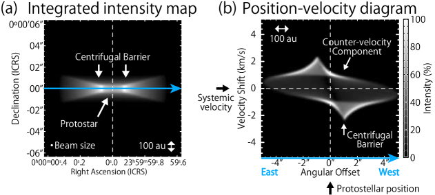
Figure 3: Examples of (a) the integrated intensity (moment 0) map and (b) the position-velocity diagram of a modeled data cube of an infalling-rotating envelope. The position axis for the position-velocity diagram is taken along the mid-plane of the envelope, which is indicated by a cyan arrow in the integrated intensity map (P.A. 270°). The parameters for the model are as follows; the distance to the object ($d$) is 100 pc, the central mass ($M$) is 0.3 $M_{\odot}$, the position angle of the disk/envelope system is 90°, the direction of the rotation is counterclockwise (1 as the input value), the outer radius ($R_{\rm out}$) is 500 au, the inner radius ($R_{\rm in}$) equals to $r_{\rm CB}$, the thickness ($H_{\rm env}$) at the protostar is 0 au, the flare angle ($F_{\rm env}$) is 30°, the power-law index of the radial density profile ($\alpha^{\rm dens}_{\rm env}$) is $-1.5$, and that of the gas-temperature distribution ($\alpha^{\rm temp}_{\rm env}$) is $0$. It should be noted that the following parameters do not affect the results, and thus their values are just set arbitrarily; the molecular density and the gas temperature at the centrifugal barrier ($n_{\rm CB}({\rm X})$) are $10^{-2}$ cm^-3 and 10 K, respectively. The emission is convolved with the intrinsic Gaussian profile with the FWHM of 0.2 km s^-1 and the Gaussian beam of ($\theta_{\rm major}$$\times$ $\theta_{\rm minor}$) $=$ (0$\farcs$2 $\times$ 0$\farcs$2) (P.A. = 0°).

Figure 3 shows an example of the infalling-rotating envelope model result. Figure 3(a) shows the integrated intensity map of the model, while Figure 3(b) shows the PV diagram along the blue arrow shown in Figure 3(a). A protostar with the central mass ($M$) of 0.3 $M_{\odot}$ is located at the central position in Figure 3(a). The distance to the protostar from the Sun ($d$) is set to be 100 pc. The envelope has an outer radius ($R_{\rm out}$) of 500 au, and the radius of the centrifugal barrier is 100 au. Note that there is no molecular emission outside $R_{\rm out}$ and inside $R_{\rm in}$ ($R_{\rm in}$ $=$ $r_{\rm CB}$) according to the specification of FERIA (Section 3.2.2). The envelope is assumed to have an edge-on configuration (inclination angle of 90°) extending along the east-west axis. The integrated intensity relative to its peak value in the panel is shown in a gray scale. The integrated intensity is the highest around the centrifugal barrier.

In the modeled PV diagram (Figure 3b), the angular offset of 0″ corresponds to the protostellar position. The vertical axis represents the line-of-sight velocity of the molecules involving the systemic velocity of the source. In Figure 3(b), a spin-up feature can be seen along the east-west axis; the rotation velocity increases as approaching to the centrifugal barrier. The velocity takes its maximum and minimum value around the centrifugal barrier, where the velocity is red-shifted and blue-shifted in the eastern and western sides of the protostellar position, respectively. Since no gas resides inside the centrifugal barrier in this model, the spin-up feature disappears at the centrifugal barrier. This is in contrast to the Keplerian disk case described later (see Section 4.2). In addition, the counter-velocity component due to the infall motion can be recognized. Toward the protostellar position, only a velocity shift due to the infall motion can be seen, since the rotation motion is perpendicular to the line of sight.

4.1 Envelope Models with Various Physical Parameters

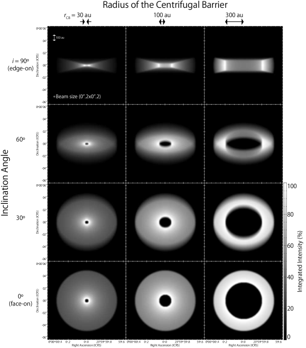
Figure 4: Examples of the integrated intensity maps of infalling-rotating envelope models. Various values of the radius of the centrifugal barrier ($r_{\rm CB}$) and the inclination angle ($i$) are employed, while the other parameters are the same as those summarized in the caption of Figure 3. The intensity is normalized by its peak value in the cube, which does not affect the appearance of the figures.

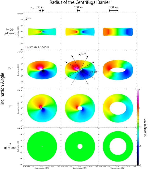
Figure 5: Examples of the velocity field (moment 1) maps of infalling-rotating envelope models. The employed parameter values for the models are summarized in the caption of Figures 3 and 4. The positions with an integrated intensity (Figure 4) lower than the 5% relative to the peak integrated intensity are masked.

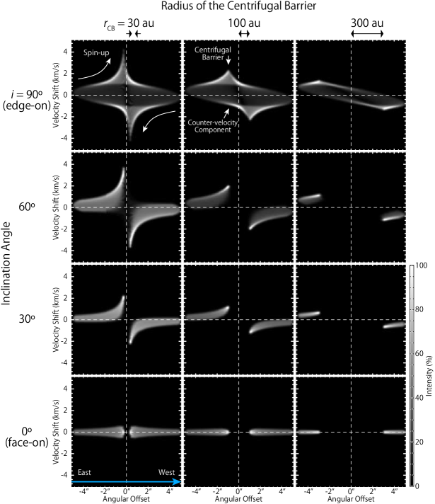
Figure 6: Examples of the position-velocity diagrams of infalling-rotating envelope models. The position axes are taken along the mid-plane of the envelopes, which is indicated by a cyan arrow in Figure 5 (P.A. 270°). The employed parameter values for the models are summarized in the caption of Figures 3 and 4.

Figures 4$-$6 show the model results with various parameter values. Figure 4 shows the integrated intensity (moment 0) maps of the models with various inclination angles ($i$) and the radii of the centrifugal barrier ($r_{\rm CB}$), while Figure 5 shows their velocity field (moment 1) maps. Figure 6 shows the PV diagrams corresponding to Figure 5. The position axis in the PV diagrams is along the mid-plane of the disk/envelope system (P.A. 270°), which is shown by the blue arrow in Figure 3(a). The other parameters are common for these models. Some parameters do not affect the calculation, as described in the caption of Figures 4$-$6, and thus they are set arbitrarily. The employed parameter values are summarized in the captions of these figures. The images are obtained by convolving the emission with the intrinsic Gaussian profile with the FWHM of 0.2 km s^-1 and the Gaussian beam of ($\theta_{\rm major}$$\times$ $\theta_{\rm minor}$) $=$ (0$\farcs$2 $\times$ 0$\farcs$2) (P.A. 0°).

In the following subsections, physical implications of some characteristic features seen in the calculated images are described. This is useful not only to understand the model but also to interpret the observed images.

4.1.1 Integrated Intensity Maps and Velocity Field Maps

In Figure 4, the maps for the edge-on configuration (a highly inclined configuration; $i$ = 90°) show double-peaked intensity distributions. At $i$ of 30° and 60°, an elliptic hole of the intensity distribution is seen. With the face-on configuration ($i$ = 0°), the intensity distributions show ring-like structures. These holes appear because there is no molecular emission inside the radius of the centrifugal barrier in this model (Section 3.2.2). For each case, the intensity takes the maximum value near the centrifugal barrier.

The velocity of the gas in the model depends on the central mass ($M$) as well as $i$ and $r_{\rm CB}$. The central mass only scales the value of velocity up and down, and it does not essentially affect the overall appearance of the velocity field map. Thus, we show the results for various $i$ and $r_{\rm CB}$ with the fixed central mass in Figure 5.

In the edge-on configuration ($i$ = 90°) case in Figure 5, the averaged velocity in the eastern and western sides of the protostar is red- and blue-shifted, respectively. These velocity shifts represent the rotation motion around the protostar. The maximum velocity shifts are seen around the centrifugal barrier, which is consistent with the velocity profile of the infalling-rotating motion (Figure 2). The velocity does not show any gradient along the north-south axis.

On the other hand, a velocity gradient along the north-south axis is seen in the panels for $i$ of 30° and 60°. These velocity gradients are due to the infall motion. As shown in Figure 1, the northern edge of the envelope is close to us in the cases with positive $i$ and a P.A. of 90°. Thus, the line emission is red-shifted in the northern side of the protostar. In these panels, the velocity fields show skewed features; the most red- and blue-shifted components are seen in the northeastern and southwestern sides of the protostar, respectively. This is because that the velocity components of the rotation and infall motion projected along the line of sight have the same direction (see Figure 1e) at these positions. Such a skewed feature was first revealed in the observation of L1551 IRS 5 by Momose et al. (1998). The results for the face-on configuration ($i$ = 0°) are trivial; the velocity shift is completely symmetric to the mid-plane of the envelope, and thus, the averaged velocity is infinitesimal everywhere.

4.1.2 Position-Velocity Diagrams

Figure 6 shows the PV diagrams along the major axis of the disk/envelope system (P.A. 270°). For the edge-on configuration ($i$ = 90°), the spin-up feature toward the centrifugal barrier is seen regardless of $r_{\rm CB}$. The maximum velocity-shift seen at the centrifugal barrier is larger for a smaller $r_{\rm CB}$, if the other parameters are fixed (see Eq. (5)). The infall motion can be confirmed as the counter-velocity components. The velocity shifts at the angular offset of 0″ (i.e. the position of the protostar) also reflect the infall motion. For $i$ of 30° and 60°, the counter-velocity components are not seen in most of panels, while they can slightly be seen in the case for $r_{\rm CB}$ of 30 au at $i$ of 60°. The gas having considerable infall motion in the models for $r_{\rm CB}$ of 100 and 300 au are distant from the protostellar position on the plane of the sky. Therefore, these components are almost outside the beam, and do not make effective contributions to these PV diagrams. Thus, investigating the velocity gradient perpendicular to the mid-plane of the disk/envelope system is essential for inclined cases, as demonstrated below and presented by Oya et al. (2016) for instance. For the face-on configuration ($i$ = 0°), it is natural that a velocity gradient due to the infall and rotation motion cannot be seen regardless of $r_{\rm CB}$.

Figure 7 shows the model results of the PV diagrams prepared along six P.A.s for $i$ of 0°, 30°, 60°, and 90°. The $r_{\rm CB}$ value is fixed to be 100 au. The P.A.s of the position axes are taken for every 30°, as shown by arrows in Figure 5. The P.A.s of ‘270°’ and ‘0°’ represent the direction along the mid-plane of the envelope and that perpendicular to it, respectively. For the edge-on configuration ($i$ = 90°), the distributions look concentrated around the protostar in all the PV diagrams except for the P.A. of 270°. A slight velocity gradient can be seen for these P.A.s, except for the P.A. of 0° (the direction perpendicular to the mid-plane). For the diagram with the P.A. of 0°, only the velocity shift due to the infall motion near the ‘centrifugal radius’ is visible, which is a half of the peak velocity-shift of the rotation motion at the centrifugal barrier (Figure 2).

At $i$ of 30° and 60°, the kinematic structure systematically changes from P.A. to P.A., which is caused by the complex combination of the rotation and infall motions. As shown in Figures 1(e) and 5, the rotation and infall motions cancel each other in the southeastern and northwestern sides of the protostar, while they strengthen each other in the northeastern and southwestern sides. For this reason, the absolute values of the velocity shift tend to be higher in the diagrams with the P.A. of 30° and 60° (southwest-northeast) than those with the P.A. of 300° and 330° (southeast-northwest). The velocity shifts due to the infall motion is seen for the P.A. of 0°. Since the infall motion has its maximum velocity at the centrifugal radius, the maximum velocity shift appears at a position with a slight offset from the protostar. For the face-on configuration ($i$ = 0°), no velocity gradient is seen for any P.A.

4.2 Comparison with the Keplerian Disk Model

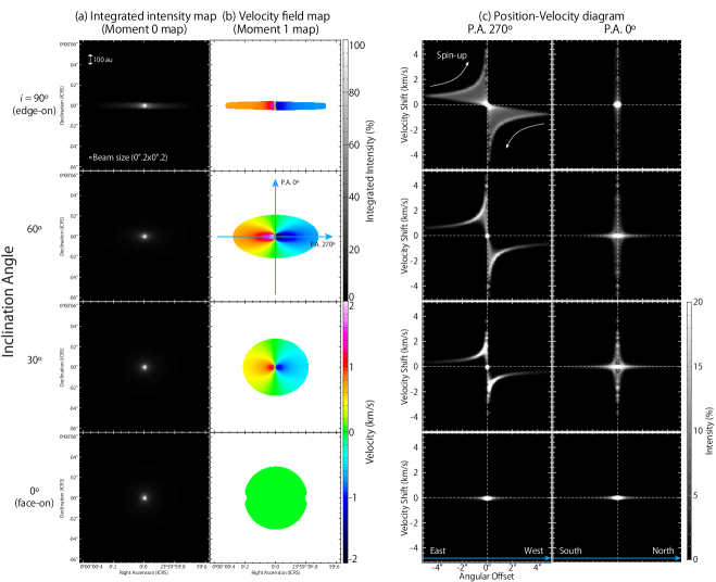
Figure 8: Examples of (a) the integrated intensity (moment 0) maps, (b) the velocity field (moment 1) maps, and (c) the position-velocity diagrams of the Keplerian disk models. The positions with an integrated intensity lower than the 5% relative to the peak value in each model are masked in the velocity field map. The position axes for the position-velocity diagrams are taken along (P.A. 270°) and perpendicular (P.A. 0°) to the mid-plane of the disks, which are indicated by cyan arrows in panel (b). The employed parameter values for the models are summarized in the caption of Figures 3 and 4, except for the $r_{\rm CB}$ and $R_{\rm in}$; $r_{\rm CB}$ is set to be larger than $R_{\rm out}$, and $R_{\rm in}$ is to be 0 au.

In analyses of rotating structures around young stellar objects, a thin-disk model with the Keplerian rotation is frequently employed. FERIA can also generate a FITS file of a data cube for the Keplerian disk (Section 3.2.2). Figure 8 shows the model results of the Keplerian disk. Although the results are trivial and well known, we present these figures to compare them with the results for the infalling-rotating motion described in Section 4.1.

In the Keplerian disk model, the velocity of the gas at the radius $r$ from the protostar is represented as;

$$v_{\rm Kep} =\sqrt{\frac{GM}{r}},\quad v_{\rm fall}=0.$$ (8)

As shown in Figure 2, the Keplerian velocity takes a smaller value than $v_{\rm rot}$ with the infalling-rotating motion by a factor of ${\displaystyle\sqrt{2}}$ at the centrifugal barrier ($r$ = $r_{\rm CB}$) for the same central mass, while it equals to $v_{\rm rot}$ and $v_{\rm fall}$ of the infalling-rotating motion at the centrifugal radius ($r$ = 2$r_{\rm CB}$).

Figure 8 shows the integrated intensity maps, the velocity field maps, and the PV diagrams of the Keplerian disk models for various inclination angles ($i$). In these models, the central mass ($M$) and the outer radius ($R_{\rm out}$) are fixed to 0.3 $M_{\odot}$ and 500 au, respectively. The constant thickness ($H_{\rm disk}$) of 50 au is assumed. The other parameters are summarized in the caption.

In the integrated intensity maps (Figure 8a), the distributions look compact and are concentrated around the protostar. Since the density of the gas is assumed to be proportional to $r^{-1.5}$ in this case, the contribution from the vicinity of the protostar is dominant. This appearance is in contrast to the infalling-rotating envelope model case described in Section 4.1.1, where the peak intensities are seen near the centrifugal barrier. In the velocity field maps (Figure 8b), the rotation motion is clearly visible. It is well-known that the velocity field of the Keplerian disk has reflection symmetry with respect to the disk mid-plane regardless of the inclination angle. This is again in contrast to the infalling-rotating envelope model case, which shows a skewed feature (Figure 5).

In the PV diagrams along the disk mid-plane (P.A. 270°), the spin-up feature is seen, except for the model with a face-on configuration ($i$ = 0°). When the kinematic structure is well resolved by a beam, no counter-velocity component is seen in contrast to the infalling-rotating envelope model case (Figure 6) because of the absence of the infall motion. In the PV diagrams along the direction perpendicular to the disk mid-plane (P.A. 0°), no velocity gradient is seen regardless of $i$, while the infalling-rotating envelope model shows a velocity gradient along this direction due to the infall motion. These different behaviors between the Keplerian disk model and the infalling-rotating envelope model correspond to the difference of their velocity field maps described above (Figures 5 and 8b). On the basis of these features, we can discriminate between the Keplerian motion and the infalling-rotating envelope in principle. However, such discrimination is not always obvious for observed data in practice, as shown later.

5 Comparison with the Actual Observations

5.1 General Aim of the Model

The infalling-rotating envelope model described in Section 2 is a quite simplified one as mentioned in Section 1; the model does not consider any excitation effects, radiative transfer effects, abundance variations of molecules, hydrodynamics effects, the effect of the self-gravity of the gas, and temporal variation of the angular momentum. In reality, the emission may be optically thick in some parts, and the distribution itself may be asymmetric around the protostar. Moreover, the infalling-rotating envelope model is not appropriate in some cases (see Section 6.2). Thus, it is not very fruitful to make a fine tuning of the model so as to better match with the observed intensity. Thus, these models have been used just for extracting the fundamental characteristics of the observed kinematic structure (e.g. Sakai et al., 2014b; Oya et al., 2016).

The advantage of FERIA is its agility and easiness to use in comparison with full hydrodynamics simulations including the above detailed effects. Thus, the analysis with using FERIA helps observers to find reasonable physical parameter values for their target sources instantly, which can be used as the initial parameters for further analyses.

5.2 Obtaining the Best Fit Parameters

In this section, we present some examples of the model analysis by using FERIA for actual observational data taken with ALMA. So far, model simulations with a wide range of physical parameters and eye-based fitting have usually been employed. We here perform unbiased evaluation of the parameter values by using the cube data.

In model analyses, chi-squared ($\chi^{2}$) tests are often employed to derive the best model parameters. For instance, Oya & Yamamoto (2020) performed the reduced $\chi^{2}$ tests for the PV diagrams. They prepared the PV diagrams of the observed line emissions and the models along the major axis of the disk mid-plane. We can perform similar tests for cube data by using FERIA. We here show trials of a $\chi^{2}$ test for the observational data toward three young low-mass protostellar sources: L1527 IRS (hereafter L1527), B335, and Elias 29. The fitting for L1527 is performed to confirm the applicability of FERIA. B335 is employed as an example for an infall-dominated system with a slight rotation motion. To the contrast, Elias 29 has been reported to have a Keplerian disk. Details of the observation and the analysis for L1527 are described in Appendix A, while those for B335 and Elias 29 were already reported by Imai et al. (2019) and Oya et al. (2019), respectively. For each target source, we prepare a data cube of a molecular line observed with ALMA concentrated in the vicinity of the protostar.

Model simulations are performed by using FERIA for various sets of the central mass ($M$) and the inclination angle ($i$) as the free parameters. As well, the radius of the centrifugal barrier ($r_{\rm CB}$) or the inner radius ($R_{\rm in}$) of the emitting region is employed as a free parameter for the infalling-rotating envelope model or the Keplerian disk model, respectively. We calculate the reduced $\chi^{2}$ values between the observed and modeled data cubes, and find the best-fit parameter values. Contribution to the reduced $\chi^{2}$ values from imperfection of the model would overwhelm those of the statistical noise. Under such a constraint, it is difficult to quantitatively discuss the likelihood for the parameter ranges. Therefore, we just demonstrate unbiased screenings for the parameter sets in this study, while further interpretation of the results of the model analyses are left for future studies on individual sources.

5.2.1 Chi-Squared Test: L1527 Case

The first case is a protostellar source whose inclination angle of the disk/envelope system is well constrained. It is L1527 IRS (IRAS 04365$+$2557), the Class 0/I protostellar source in Taurus. The disk/envelope system of L1527 has an almost edge-on configuration with the inclination angle of 95° (Tobin et al., 2013; Oya et al., 2015). This source is already known to have the infalling-rotating envelope based on the previous observational studies. The infalling-rotating motion of the gas has been detected in various molecular lines: C¹⁸O by Ohashi et al. (2014) and Aso et al. (2017), c-C_3H_2 and CCH by Sakai et al. (2014a, b), and CS by Oya et al. (2015). Thus, this source is a good test case to confirm that FERIA works for the actual observation data.

We perform a $\chi^{2}$ test for the CS ($J=3-2$) emission observed with ALMA (see Appendix A). The CS emission is suitable for this study, because it is known to trace the disk/envelope system of L1527 (Oya et al., 2015) and to be free from the contamination by other molecular lines. Moreover, our CS ($J=3-2$) data observed in ALMA Cycle 4 have a better quality than the CS ($J=5-4$) data in ALMA Cycle 0 reported by Sakai et al. (2014b) and Oya et al. (2015). The free parameters for each case are summarized in Table 2. The inclination angle ($i$) of 95° is employed according to the previous reports (Tobin et al., 2013; Oya et al., 2015), where the western side of the disk/envelope system faces us (Oya et al., 2015). $R_{\rm out}$ is fixed to be 500 au according to the distribution of the CS emission. The distance ($d$) of 137 pc is employed for the consistency with our previous report (Oya et al., 2015). The emission in the following models is convolved with the Gaussian beam of 0$\farcs$459 $\times$ 0$\farcs$400 (P.A. $-20.098$°) and the intrinsic line width of 0.5 km s^-1. Since there is a contamination from the outflow component in the CS emission, only the data points within the specified region and the velocity range are considered (Figures 9a, 11a).

The $\chi^{2}$ test is performed for the model of the infalling-rotating envelope, according to the aforementioned previous reports. The free parameters for the $\chi^{2}$ test are the protostellar mass ($M$) and the radius of the centrifugal barrier ($r_{\rm CB}$). Their values for the best-fit model are summarized in Table 2.

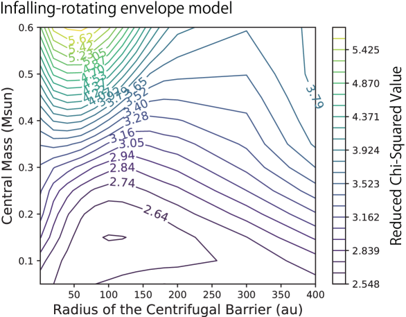
Figure 12: Reduced $\chi^{2}$ map with various parameter values for L1527. Free parameters and their ranges are summarized in Table 2.

The best-fit model is compared with the observation in Figures 9$-$11. The obtained infalling-rotating envelope model reasonably reproduces the observed flattened distribution in the integrated intensity map. As well, the velocity gradient along the north-south direction in the observation is reproduced. Figure 12 shows the reduced $\chi^{2}$ map for the various values for the two free parameters. The central mass ($M$) seems well constrained with the infalling-rotating envelope model.

It is notable that the values obtained in this analysis ($M$ of 0.15 $M_{\odot}$, $r_{\rm CB}$ of 100 au) are reasonably consistent with the previous reports; for instance, Sakai et al. (2014a) assumed $M$ of 0.18 $M_{\odot}$ and $r_{\rm CB}$ of 100 au based on the morphology in one PV diagram prepared along the mid-plane of the envelope. Our analysis taking the PPV (cube) data into account indeed reproduces the previous result.

5.2.2 Chi-Squared Test: B335 Case

The second case is a source with a very small rotation motion. B335 is a Bok globule harboring a low-mass Class 0 protostar IRAS 19347$+$0727 (Keene et al., 1980). This is an isolated source, and thus, its physical and kinematic structures have extensively been studied as a good test bed of the protostellar evolution studies (e.g. Hirano et al., 1988, 1992; Chandler & Sargent, 1993; Zhou et al., 1993; Wilner et al., 2000; Harvey et al., 2001; Yen et al., 2020; Cabedo et al., 2021). Evans et al. (2015) and Yen et al. (2015) detected the infall motion of the gas associated with the protostar with ALMA. The small rotation motion on a 10-au scale in its disk/envelope system was investigated with ALMA at resolutions of 10 au and 3 au by Imai et al. (2019) and Bjerkeli et al. (2019), respectively. Imai et al. (2019) reported that the PV diagram observed at a 10 au resolution is better fitted by the infalling-rotating motion than the Keplerian motion, and they derived the protostellar mass of $(0.02-0.06)$ $M_{\odot}$. Meanwhile, Bjerkeli et al. (2019) just assumed the Keplerian motion and derived the protostellar mass to be 0.05 $M_{\odot}$ by using the PV diagram of their data. Hence, the origin of the rotation motion in this source is still controversial. A nearly edge-on geometry is preferable for B335 based on its outflow geometry (Hirano et al., 1988; Yen et al., 2010; Imai et al., 2016; Bjerkeli et al., 2019).

We perform a $\chi^{2}$ test for the infalling-rotating envelope model and the Keplerian disk model on the cube data of the CH_3OH ($12_{6,7}-13_{5,8}$; E) emission reported by Imai et al. (2019). They reported that this molecular line traces the marginal rotation motion in B335. The free parameters for each case are summarized in Table 3. $R_{\rm out}$ is fixed to 10 au according to the distribution of the CH_3OH emission. The distance ($d$) to B335 was reported to be 100 pc by Olofsson & Olofsson (2009), and was later updated to be 164.5 pc by Watson (2020). We employ the former for the consistency with the previous work by Imai et al. (2019). The emission in the following models is convolved with the Gaussian beam of 0$\farcs$116 $\times$ 0$\farcs$082 (P.A. $-56.692$°) and the intrinsic line width of 1.0 km s^-1.

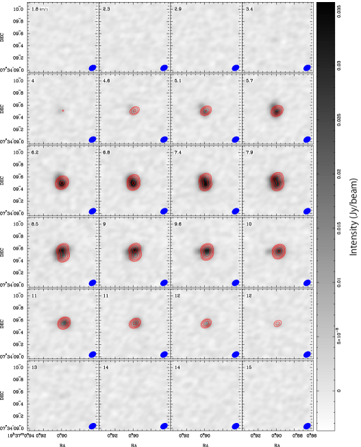
Figure 14: Comparison of the velocity channel maps between the observation and the results of the infalling-rotating envelope model for B335 (see Section 5.2.2). Grey scale maps represent the observed CH_3OH ($12_{6,7}-13_{5,8}$; E) emission. Contours represent the best-fit model obtained by the $\chi^{2}$ test for the infalling-rotating envelope model. The parameters for the model are: $M$ of 0.02 $M_{\odot}$, $r_{\rm CB}$ of 1 au, and $i$ of 70°. Contour levels are 5%, 10%, 20%, 40%, and 80% of the peak intensity of the model. The original channel width of 0.28 km s^-1 is used in the $\chi^{2}$ test, whereas the two successive channels are combined in these velocity channel maps. The central velocity is shown at the upper left corner of each panel. The beam size is depicted at the bottom right corner of each panel.

The best-fit models are compared with the observation in Figures 13$-$16. The observed CH_3OH ($12_{6,7}-13_{5,8}$; E) emission has a compact and almost circular distribution, which is reproduced by the two models (Figures 13a$-$c). Imai et al. (2019) detected the velocity gradient along the northwest-southeast direction (Figure 13d), which is tilted from the mid-plane of the disk/envelope system along the north-south direction, and attributed it to the infall motion of the gas. It is indeed reproduced by the infalling-rotating envelope model (Figure 13e). The channel maps of the models seem to reasonably reproduce the observation in Figures 14 and 15. Figure 16 shows the PV diagrams along the mid-plane of the disk/envelope system; a velocity gradient due to the small rotation motion is fortunately detected in the observation, and it is reproduced by either model.

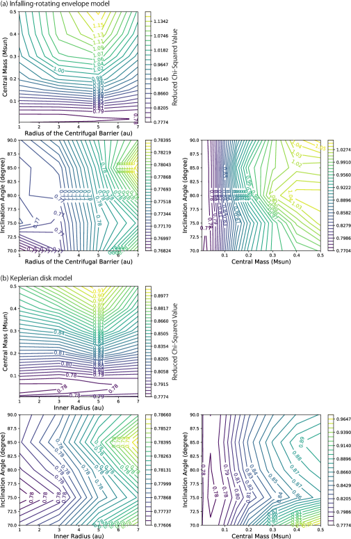
Figure 17: Reduced $\chi^{2}$ maps with various parameter values for B335. Free parameters and their ranges are summarized in Table 3.

Figure 17 shows the reduced $\chi^{2}$ maps for various parameter values. The protostellar mass is reasonably constrained by either model. $r_{\rm CB}$ and $R_{\rm in}$ are also constrained, while the inclination angle is not. Although the rotation motion of the gas in B335 is marginal in the observation, the analysis with the models is found to be useful to constrain the physical parametes.

The best-fit results for the infalling-rotating envelope model and the Keplerian disk model are summarized in Table 3. The lowest reduced $\chi^{2}$ values for these two case are comparable; the kinematic structure observed in the CH_3OH ($12_{6,7}-13_{5,8}$; E) emission can be approximated by either kinematic structure. The small rotation motion in B335 is indeed reflected in the parameters of the models: the small central mass ($M$) and the small radius of the centrifugal barrier ($r_{\rm CB}$).

The maximum-likelihood value of $M$ for the best-fit models are different between the infalling-rotating envelope model and the Keplerian model (Table 3); smaller $M$ is obtained for the infalling-rotating envelope model. This is a natural consequence of the different formulation of the models, where the mass estimated from the rotation velocity at the centrifugal barrier by assuming the infalling-rotating motion is the half of that estimated by assuming the Keplerian motion (see Eqs. (5) and (8)).

5.2.3 Chi-Squared Test: Elias 29 Case

The third case is a source with an ordinary inclination angle. Elias 29 is the Class I protostellar source in Ophiuchus. In this source, the rotation motion of the gas associated with its protostar was detected in the SO ($J_{N}=6_{7}-5_{6}$) emission by Oya et al. (2019). They reported that the observed kinematic structure is reasonably explained by the Keplerian disk model, where $M$ is 1.0 $M_{\odot}$, $i$ is 65°, and $R_{\rm out}$ is 100 au. In their report, the mid-plane of the disk/envelope system is assumed to lie along the north-south direction (P.A. 0°). It was reported that a fully face-on configuration ($i$ = 0°) is unlikely for Elias 29 (Lommen et al., 2008), and the inclination angle was constrained to be from 65° to 115° (Oya et al., 2019).

Elias 29 is a relatively evolved Class I source judging from its high bolometric temperature (Miotello et al., 2014). Thus, it is naturally expected to have a Keplerian disk, as assumed by Oya et al. (2019). However, is this really the case? In this study, we examine a possibility of an infall motion in this source as well as that of a Keplerian motion with the aid of FERIA.

We perform a $\chi^{2}$ test for the SO ($J_{N}=6_{7}-5_{6}$) data reported by Oya et al. (2019). The free parameters for the infalling-rotating envelope model and the Keplerian disk model are summarized in Table 4. $R_{\rm out}$ is fixed to be 50 au according to the distribution of the SO emission. The distance ($d$) to Elias 29 was reported to be $(137-147)$ pc by Ortiz-León et al. (2017) and $141^{+30}_{-21}$ pc by Dzib et al. (2018). We employ $d$ of 137 pc in this study for the consistency with our previous work (Oya et al., 2019). We assume that the mid-plane of the disk/envelope system of Elias 29 extends along the northeast-southwest direction with the position angle of 30°, judging from the outflow directions (Ceccarelli et al., 2002; Ybarra et al., 2006; Bussmann et al., 2007). The emission in the following models is convolved with the Gaussian beam of 0$\farcs$832 $\times$ 0$\farcs$488 (P.A. $-85.833$°) and the intrinsic line width of 1.0 km s^-1.

The best-fit results for the infalling-rotating envelope model and the Keplerian disk model are summarized in Table 4. Again, $M$ is obtained to be smaller for the infalling-rotating envelope model (0.6 $M_{\odot}$) than the Keplerian disk model (1.4 $M_{\odot}$). This difference can mainly be interpreted as the expected difference by a factor of 2 following Eqs. (5) and (8), as described in Section 5.2.2, although the different inclination angles between both models also contribute to the difference.

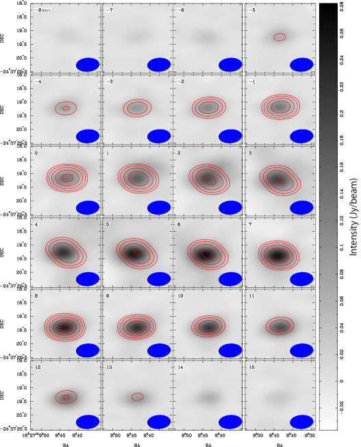
Figure 19: Comparison of the velocity channel maps between the observation and the results of the infalling-rotating envelope model for Elias 29 (see Section 5.2.3). Grey scale maps represent the observed SO ($J_{N}=6_{7}-5_{6}$) emission. Contours represent the best-fit model obtained by the $\chi^{2}$ test for the infalling-rotating envelope model. The parameters for the model are: $M$ of 0.6 $M_{\odot}$, $r_{\rm CB}$ of 5 au, and $i$ of 120°. Contour levels are 5%, 10%, 20%, 40%, and 80% of the peak intensity of the model. The original channel width of 0.2 km s^-1 is used in the $\chi^{2}$ test, whereas the five successive channels are combined in these velocity channel maps. The central velocity is shown at the upper left corner of each panel. The beam size is depicted at the bottom right corner of each panel.

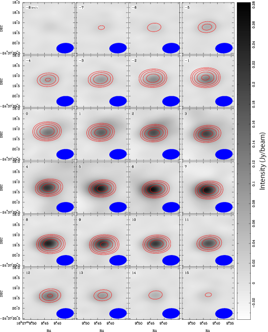
Figure 20: Same as Figure 19, but for the Keplerian disk model. Contours represent the best-fit model obtained by the $\chi^{2}$ test for the Keplerian disk model. The parameters for the model are: $M$ of 1.4 $M_{\odot}$, $R_{\rm in}$ of 1 au, and $i$ of 80°.

The best-fit models are compared with the observation in Figures 18$-$21. The observed SO ($J_{N}=6_{7}-5_{6}$) emission has an elliptic distribution tracing the disk/envelope system, which is reproduced by both models (Figures 18a$-$c). As well, the velocity gradient along the north-south direction in the observation is reproduced by the models (Figures 18e$-$g). A skewed velocity feature with respect to the mid-plane direction (the red line in Figure 18a; P.A. 30°) is marginally seen in the observation (Figure 18e). This trend seems a bit overemphasized in the infalling-rotating envelope model (Figure 18f). In contrast, the Keplerian model shows a velocity gradient rather close to the mid-plane direction. The feature seen in the northwestern and southeastern parts of the Keplerian model would not be robust; it is interpreted as the effect of the large flat beam, because it does not appear with a small circular beam (Figure 8). The channel maps are shown in Figures 19 and 20, and the PV diagrams along the mid-plane of the disk/envelope system are in Figure 21. A small difference of the reduced $\chi^{2}$ values (Table 4) suggests that the observed kinematic structure is explained by either model.

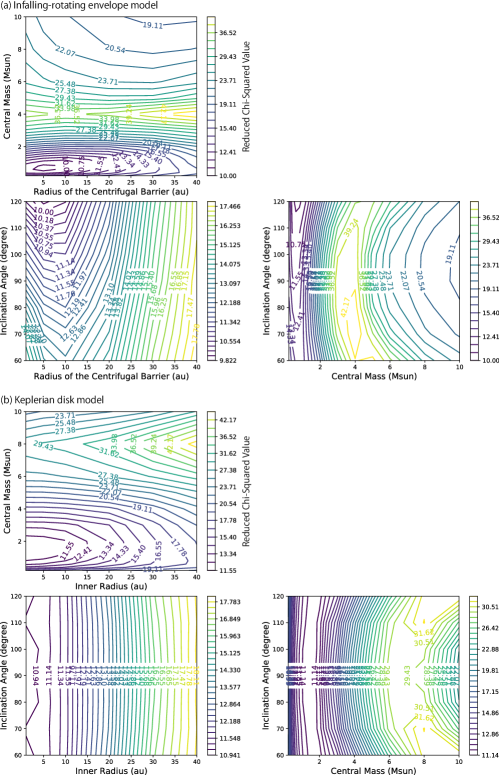
Figure 22: Reduced $\chi^{2}$ maps with various parameter values for Elias 29. Free parameters and their ranges are summarized in Table 4.

Figure 22 shows the reduced $\chi^{2}$ maps for various parameter values. The central mass ($M$) seems well constrained in both the two cases. The radius of the centrifugal barrier ($r_{\rm CB}$) or the inner radius of the disk ($R_{\rm in}$) are estimated to be much smaller than the beam size (0$\farcs$8 $\times$ 0$\farcs$5 $\sim$ 100 au). Meanwhile, the inclination angle ($i$) is poorly constrained in this analysis. Further discussion for the disk/envelope system of Elias 29 would become possible when $i$ is constrained by other approaches, for instance the analysis of the outflow structure.

It should be noted that the lowest reduced $\chi^{2}$ value is smaller for the infalling-rotating envelope model than the Keplerian model by 10%. This slight difference may not have a statistical meaning due to the overwhelming contribution from the simple assumptions in the models. Nevertheless, an infalling motion may contribute to the kinematic structure of Elias 29 in addition to a pure Keplerian motion previously assumed by Oya et al. (2019).

Based on the above results, one may think that the actual situation would be the hybrid case of the infalling-rotating motion and Keplerian motion. Since FERIA can simulate such a hybrid case by the combined model, we here present a preliminary attempt to apply it for the observed data to see how it works. The results will be useful for the user of FERIA to apply the combined model for more complicated systems.

As a demonstration, the combined model is compared with the observation for Elias 29. In this model, the gas within the radius of the centrifugal barrier ($r_{\rm CB}$) is assumed to be the Keplerian disk. The inner radius ($R_{\rm in}$) is fixed to be 1 au to reduce the parameter space. The result of the reduced $\chi^{2}$ test is summarized in Table 4. The obtained $r_{\rm CB}$ of 10 au suggests that there are both the contribution from the infalling-rotating envelope and the Keplerian disk. The best-fit model is compared with the observational result in Figures 18(d, h), 21(d), and 23.

As summarized in Table 4, the fitting is slightly improved with the combined model compared with the results for the infalling-rotating envelope model and the Keplerian model. However, the improvement of $\chi^{2}$ value is too small to conclude that the obtained values with the combined model reflect the actual physical conditions. Our result indicates that the disk-forming region of this source needs to be further characterized with a higher angular-resolution observations in the future.

5.2.4 Chi-Squared Test: Discussion

In previous works, the observed kinematic structures have typically been analyzed in 2-dimensional manners; for instance, PV diagrams or velocity profiles, as described in the above sections. Such analyses often effectively focus on the characteristic features in the observations, and it have helped us to constrain the physical parameters, such as the protostellar mass. However, these analyses arbitrarily prune much information of the 3-dimensional cube data for simplicity. Such dimensional reduction may provide a biased view on the kinematic structure. Thus, using all the 3-dimensional information is preferred to characterize the observed kinematic structure. FERIA makes such comparison of the 3-dimensional data easier.

In the above sections, the $\chi^{2}$ test is applied for the 3-dimensional cube data for the three sources. We find that it is difficult to discriminate the infalling-rotating motion and the Keplerian rotation for B335 and Elias 29. For these cases, the rotation structures are not well resolved, and higher spatial resolution observations may work for definitive discrimination. The results for B335 and Elias 29 also imply that we should not too much rely on the $\chi^{2}$ test of a single molecular line for discrimination. Limited quality and limited resolutions of the data as well as contamination of the outflow components may affect the result.

Since some molecular emissions selectively trace a particular part of the disk/envelope structure just as molecular markers (Sakai et al., 2014b; Oya et al., 2016, 2017; Oya, 2020; Oya & Yamamoto, 2020), selection of molecular lines in advance is very important. Model analyses would get more successful by applying to molecular lines whose kinematic structures are classified into the infalling-rotating motion or the Keplerian rotation in preprocess. Based on multiple-molecular-line analyses, comprehensive consideration should be made for full understanding of the disk/envelope structure. With this in mind, we present a possible approach to classification of molecular lines in the next section, as another application of FERIA.

5.3 Combination with Machine/Deep Learnings

In the last decade, a plenty of observational data of ALMA have been archived for open use. Some of them have a high spatial and velocity resolutions enough to trace the kinematic structure in the vicinity of a protostar. With such a flood of observational data, it gets more and more important to analyze them effectively and automatically. In this context, it would be effective to adopt machine/deep learnings for analyzing the observational data (see Baron, 2019).

In fact, for instance, the principal component analysis (PCA) is often employed to analyze observational data in an unbiased way (e.g. Ungerechts et al., 1997; Meier & Turner, 2005; Neufeld et al., 2007; Watanabe et al., 2016; Spezzano et al., 2017; Okoda et al., 2020, 2021). It is an unsupervised machine learning algorithm for dimensionality reduction (Jolliffe, 1986). Moreover, deep learning algorithms such as the convolutional neutral networks (CNN) and the conditional generative adversarial networks (cGAN) (e.g. Gillet et al., 2019; Shirasaki et al., 2019; Moriwaki et al., 2020) have recently been employed. These previous works using machine learnings and deep learnings were mostly performed for intensity distributions or line spectra, i.e. mainly for the studies of the morphology of objects or the chemical composition. On the other hand, there are still no successful attempt for the gas kinematics in protostellar sources as far as we know.

FERIA can generate one cube FITS file in a 10s seconds. It allows us to readily prepare a heap of mock data cubes, which can be used as the training datasets for supervised learnings. A possible application is the classification of the observed gas kinematic structure into the infalling-rotating envelope motion and the Keplerian motion in the three-dimensional coordinate. Support vector classification (SVC) and three-dimensional convolutional neural network (3DCNN) are candidate supervised learning algorithms for this purpose. Since the actual gas motion is often not pure ballistic nor pure Keplerian, the classification may not be perfect. Nevertheless, such automatic discrimination between them, if possible, will be useful to deal with a large observational data as an initial classification for further detailed inspection.

We here present such an analysis with SVC to classify the infalling-rotating motion and the Keplerian motion. Hereafter, we employ the stochastic gradient descent (SGD) algorithm to train the classifier by using the library provided by SCIKIT-LEARN. We apply this analysis method to the ALMA observations toward 49 Ceti and IRAS 16293$-$2422 Source A.

5.3.1 Analysis with Support Vector Classification: 49 Ceti Case

First, we apply the above analysis method to the ALMA observation toward the debris disk of 49 Ceti. Since the CO and [CI] emissions clearly trace the Keplerian motion in this source (Higuchi et al., 2019), they can be used as a good test case to assess the usability of this analysis method.

By using FERIA, we first prepare 9180 infalling-rotating envelope models and 9180 Keplerian disk models as the mock data set, which are simulated by using various combination of the central mass ($M$), the inclination angle ($i$), and the outer radius ($R_{\rm out}$), as summarized in Table 5. In addition, the radius of the centrifugal barrier ($r_{\rm CB}$) or the inner radius ($R_{\rm in}$) is added in the combinations for an infalling-rotating envelope or a Keplerian disk, respectively. Note that values of $r_{\rm CB}$ and $R_{\rm in}$ are employed only if they are smaller than $R_{\rm out}$. The other parameters are fixed according to the characteristics of 49 Ceti in order to reduce the parameter space; for instance, we employ $-72\arcdeg$ as the P.A. of its disk mid-plane (Higuchi et al., 2019). 80% among the mock data are randomly picked up and are used as the training and validation data sets. The quality of the trained classifier is assessed by testing with the remaining 20% mock data as the evaluation data set. The confusion matrix of this evaluation is shown in Table 6. The trained classifier marks the accuracy as high as 99.9%, where only 4 mock data are wrongly classified. Two of the wrongly classified mock data have the completely face-on configuration ($i$ of 0° or 180°), and the other two have the smallest central mass ($M$ of 0.50 $M_{\odot}$) in the parameter range (Table 5). Because they have small velocity shifts, the kinematic structures are not well resolved in the modeled data cubes. Thus, these 4 mock data are recognized as outliers among the mock data, which are difficult to classify. Therefore, the trained classifier is enough accurate to classify the two kinematic structures for ordinary cases.

Then, we apply this classifier to the actual data cubes of the CO and [CI] emissions observed with ALMA (Higuchi et al., 2019). The classifier successfully classifies the kinematic structure of these two molecular emissions as the Keplerian motion as expected. Therefore, this approach with a machine learning seems to work on the actual observation data.

5.3.2 Analysis with Support Vector Classification: IRAS 16293$-$2422 Case

Second, we apply this analysis method to the ALMA observation toward the Class 0 protostellar source IRAS 16293$-$2422 Source A, which is a binary or multiple system. According to Oya & Yamamoto (2020), the C^17O and H_2CS emissions trace its circummultiple structure and circumstellar disk, respectively.

We first prepared 14400 infalling-rotating envelope models and 14400 Keplerian disk models as the mock data set, whose parameter ranges are summarized in Table 5. Values of $r_{\rm CB}$ and $R_{\rm in}$ are employed only if they are smaller than $R_{\rm out}$. We employ $50\arcdeg$ as the P.A. of the disk/envelope mid-plane of IRAS 16293$-$2422 Source A (Oya & Yamamoto, 2020). Although Oya & Yamamoto (2020) reported that the gravitational centers for the circummultiple and circumstellar structures are slightly offset from each other, we employ the centeral position for the circummultiple structure as that for all the mock data in this study. Again, 80% of the mock data set are used to train and tune the classifier, and the other 20% are to evaluate it. The confusion matrix is shown in Table 7. The classification accuracy is as high as 98.9%, and thus this classifier works well. The classification is failed for 62 mock data out of 5760 mock data; they seem to be outliers among the mock data as we found in the analysis for the 49 Ceti. 37 of the 62 mock data have the completely face-on configuration, and 10 of the others have the smallest central mass ($M$ of 0.1 $M_{\odot}$; Table 5). In the other 15 mock data, the radius of the centrifugal barrier ($r_{\rm CB}$) and the outer radius ($R_{\rm out}$) are close to each other; for instance, $r_{\rm CB}$ of 140 au and $R_{\rm out}$ of 150 au. These mock data have only small emitting regions, and the classification may be difficult by the present method.

Then, we apply it to the actual data cubes of the molecular emissions observed with ALMA, where the details of the observation were reported by Oya & Yamamoto (2020) and Oya et al. (2021). The results are summarized in Table 8. The C^17O emission is successfully classified to the infalling-rotating envelope as previously reported (Oya & Yamamoto, 2020). The H_2CS emission, which comes from both the circummultiple structure with the infalling-rotating motion and the circumstellar disk with the Keplerian motion, is also classified to the infalling-rotating envelope. As well, all the other molecular lines except for the (CH_3)_2CO emission are classified to the infalling-rotating envelope. A reason for this result would be that the contribution of the extended circummultiple structure is overwhelming for most molecular lines in comparison with the compact circumstellar disk. In contrast, the (CH_3)_2CO emission is expected to be suitable to investigate the circumstellar disk without the contamination from the circummultiple structure, and thus, its further investigation is awaited. Unbiased analyses with machine/deep learnings and model calculations are potentially useful to find out such unique cases. In addition, a survey for molecular species classified as the Keplerian disk is essential to study the disk chemistry in this source.

In this section, we have presented just a tentative demonstration of the analysis method using a machine learning SVC by using the mock data produced by FERIA. Utility of analyses introducing machine/deep learnings will rapidly be enhanced in the future with expanding archival observation data. We would like to emphasize that the agility and simpleness of FERIA are quite advantageous in preparing a huge pile of model dataset for such analyses.

6 Discussion

6.1 Why Is the Model Applicable?

While the infalling-rotating motion has long been considered (e.g. Ohashi et al., 1997), the concept of its centrifugal barrier was first reported in the ALMA observation by Sakai et al. (2014a), and was formulated and modeled by Oya et al. (2014). An existence of the centrifugal barrier is naturally expected from simple assumptions of the energy and the angular momentum conservation. In fact, its identification or hint was confirmed in observations of other young low-mass protostellar sources (e.g. Oya et al., 2014, 2016, 2017, 2018a; Sakai et al., 2016; Lee et al., 2017; Alves et al., 2017; Imai et al., 2019, 2022). Moreover, disk structures seem to be formed inside the centrifugal barriers even at the earliest evolutionary stages (Classes 0-I). The centrifugal barrier can be regarded as a boundary between the infalling-rotating envelope outside it and the disk component inside it. In reality, the transition zone from an envelope to a disk would extend over a considerable size near the centrifugal barrier, and the envelope and the disk may intricately be contaminated with each other there. Numerical MHD calculation indeed show a complex structure of the transition zone in the disk forming region, which depends on assumed physical conditions. Nevertheless, the infalling-rotating envelope model well represents the kinematic structure of such regions at least in some sources mentioned above, where the centrifugal barrier stands for an approximate position of the transition zone.

Generally, the size of a rotationally-supported disk, or a Keplerian disk, is thought to correspond to the ‘centrifugal radius’ (Hartmann, 2009). It is the radius where the centrifugal force of the gas and the gravity under the central mass are balanced out, and is twice the radius of the centrifugal barrier (Section 2.2). Thus, the gas can stably keep rotation around the protostar at the centrifugal radius. The angular momentum of the gas infalling at a later time tends to be larger, which makes the centrifugal radius larger. This situation results in the smooth growth of the disk.

However, it seems to be a rather quasi-static picture. In an infalling-rotating envelope, the rotation speed equals to the infall speed at the centrifugal radius. Since the rotation speed is the same as the Keplerian speed there, the rotation motion can be continuous from the infalling-rotating envelope to the Keplerian disk at the centrifugal radius. On the other hand, there remains the infall motion as far as the effect of the gas pressure and the magnetic field are not significant (see below), and the infalling gas tends to go further inward of the centrifugal radius. In this case, the gas components between the $r_{\rm CR}$ and $r_{\rm CB}$ has a rotating speed higher than the Keplerian speed. A hint of such a ‘super-Kepler’ like component is seen, for instance, in the numerical simulations by Machida et al. (2011) (their Figure 4) and Zhao et al. (2016) (their Figures 11 and 15). Although Figure 4 of Machida et al. (2011) reveals that the motion is mostly represented by the Keplerian motion, it also shows some cases where the rotation velocity slightly exceeds the Keplerian velocity in the transition zone from the envelope to the disk. This implies an intrinsic complexity of the transition zone. According to Zhao et al. (2016), a weak magnetic coupling due to removal of small dust grains is responsible for such a feature.

Some observational results indeed indicate that the gas apparently keeps falling beyond the centrifugal radius toward the centrifugal barrier (e.g. Sakai et al., 2014b; Oya et al., 2016), and they have been reasonably reproduced by the infalling-rotating envelope model. Furthermore, a jump of the rotation speed down to the Keplerian speed around the centrifugal barrier is also suggested in the H_2CO observation toward BHB 07$-$11 by Alves et al. (2017). Thus, phenomenologically speaking, the infalling-rotating envelope model captures an essence of the kinematic structure of the envelope and the transition zone at least partly.

Although the infalling-rotating envelope model reproduces a major observed feature of the gas kinematics, we should note that this is a very simplified model. In more realistic cases, the infall motion of the gas will be suppressed due to the gas pressure. This effect is, however, not always effective near the centrifugal radius. The static ($P_{\rm stat}$) and dynamic ($P_{\rm dyn}$) pressures of the gas are represented as follows (e.g. Chandrasekhar & Fermi, 1953b; Hartmann, 2009):

$$P_{\rm stat} =\rho c_{s}^{2},$$ (9)

$$P_{\rm dyn} =\frac{1}{2}\rho v_{\rm fall}^{2}$$ (10)

where $\rho$, $c_{s}$, and $v_{\rm fall}$ denote the mass density of the gas, the sound speed, and the radial velocity of the gas motion, respectively. Thus, if $\rho$ can be assumed to be locally constant, the dynamic pressure is larger than the static pressure if $v_{\rm fall}$ is larger than $\sqrt{2}c_{s}$. Therefore, the gas is hardly supported by the static pressure for the case of a large $v_{\rm fall}$, and keeps falling beyond the centrifugal radius toward the centrifugal barrier to some extent.

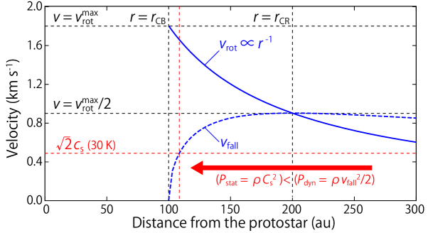
Figure 24: Velocity profile in the infalling-rotating envelope model for L1527 (Sakai et al., 2014b; Oya et al., 2015). In the infalling-rotating envelope model, the infall velocity takes its maximum value ($v_{\rm fall}$$=0.9$ km s^-1) at the centrifugal radius ($r_{\rm CR}$ $=200$ au). The sound speed $c_{\rm s}$ is assumed to be 0.35 km s^-1, which corresponds to the value at the temperature of 30 K. We here employ the protostellar mass of 0.18 $M_{\odot}$ and the radius of the centrifugal barrier of 100 au according to the report by Sakai et al. (2014a).

As for the L1527 case (Section 5.2.1; Sakai et al., 2014a, b), such a condition is expected to be fulfilled until the gas reaches near the centrifugal barrier, as shown in Figure 24. In fact, the static and dynamic pressures are roughly evaluated to be $0.5\times 10^{-6}$ and $1.6\times 10^{-6}$ dyn cm^-2 at the centrifugal radius, respectively, where the $v_{\rm fall}$ is 0.9 km s^-1. Here, we employed $M$ of 0.18 $M_{\odot}$ and $r_{\rm CB}$ of 100 au reported by Sakai et al. (2014a) instead of the rough evaluation in the trial of the $\chi^{2}$ test described in Section 5.2.1. The gas number density is assumed to be $10^{8}$ cm^-3, and the averaged particle mass to be $3.83\times 10^{-24}$ g. $c_{s}$ is proportional to ${\displaystyle\sqrt{T}}$, where $T$ is the gas temperature. It is calculated to be 0.35 km s^-1 for the gas temperature of 30 K in the infalling-rotating envelope of L1527 (Sakai et al., 2014a).

On the other hand, the magnetic pressure is represented as:

$$P_{M} =\frac{B^{2}}{2\mu_{0}},$$ (11)

where $B$ is the magnetic field and $\mu_{0}$ the magnetic permeability (Chandrasekhar & Fermi, 1953a). Then, we obtain the following practical expression:

$$P_{M} =3.98\times 10^{-14}B\left(\mu G\right)^{2}{\rm dyn\ cm}^{-2}.$$ (12)

Hence, the magnetic pressure can be comparable to the dynamic pressure, only when the magnetic field is of the order of 10 mG. In turn, the infalling-rotating envelope model does not work under such a high magnetic field condition. The magnetic field strength in the transition zone has not been well understood observationally, although the effect of the magnetic breaking has often been invoked to account the infall motion (e.g. Machida et al., 2014; Aso et al., 2015; Yen et al., 2017). It should be noted that the ratio of the magnetic pressure to the static gas pressure is assumed to be unity or less in the MHD calculations (e.g. Machida et al., 2011), otherwise the disk/envelope sturucture would be unstable (Shibata et al., 1990; Machida et al., 2000). Therefore, it is not clear how the magnetic pressure contributes to the force balance around the centrifugal radius.

Since $\rho$ and $c_{s}$ will be increased around the centrifugal barrier due to the stagnation of the gas and the relatively high temperature at the centrifugal barrier (60 K in L1527, $>$300 K in IRAS 16293$-$2422; Sakai et al., 2014b; Oya et al., 2016) in comparison with the temperature in the infalling-rotating envelope (30 K in L1527, $<$200 K in IRAS 16293$-$2422), the static pressure will be enhanced near the centrifugal barrier. Thus, the gas may stop falling before it reaches at the centrifugal barrier. This means that the edge of the rotationally supported disk will be somewhere between the centrifugal radius and the centrifugal barrier.

Within the $r_{\rm CB}$, FERIA assumes a disk component. This is justified by the following considerations. Because of the gradual increase of the specific angular momentum of the infall gas described above, the gas accreted before would have a smaller $r_{\rm CB}$ than the $r_{\rm CB}$ for the currently accreting gas (see Eq. (1)). This allows the existence of a disk component within the current $r_{\rm CB}$. Moreover, the angular momentum of the gas would be removed from the stagnated gas around the centrifugal barrier, which would help the transition of the infall gas to the rotationally-supported gas. This process is also potentially related to the outflow launching (see Section 6.3), which has been studied observationally by Oya et al. (2015, 2018b, 2021). The angular momentum of the accreting gas is transferred to the rotation of the outflowing gas (e.g. Blandford & Payne, 1982; Tomisaka, 2000; Anderson et al., 2003; Pudritz et al., 2007; Machida & Hosokawa, 2013) (see Section 6.3). The mechanism of this kinematic transition occurring from $r_{\rm CR}$/$r_{\rm CB}$ toward the disk is the remaining important issue for full understandings of the disk formation.

6.2 Caveats for Employing the Model

Although the infalling-rotating envelope model has successfully been employed to investigate the observed kinematic structures, we expect some cases for which the infalling-rotating envelope model could not be applied.

The effects of the gas pressure and the magnetic pressure described above may not be negligible in some sources. The magnetic breaking effect could be overwhelming near the protostar, and the infalling gas would be stagnated before it reaches the centrifugal barrier. As well, very young protostellar sources are not appropriate for FERIA. In such sources, the envelope mass is not negligible in comparison with the central mass. Thus, the self-gravity of the envelope gas needs to be considered, which is not taken into account in FERIA.

In addition, sources with a very small or high central mass are not appropriate for the infalling-rotating envelope model. With a small central mass, the infall velocity is so small that the dynamic pressure of the gas is small. This will result in the situation that the static pressure around the centrifugal radius is higher than the dynamic pressure. For instance, the Class 0 protostellar source IRAS 15398$-$3359 is reported to have a central mass as small as 0.007 $M_{\odot}$ (Okoda et al., 2018), resulting in the infall velocity of 0.3 km s^-1 at its centrifugal radius (80 au). In this case, the dynamic pressure of ${\displaystyle\left(0.2\times 10^{-6}\right)}$ dyn cm^-2 does not overwhelm the static pressure of ${\displaystyle\left(0.5\times 10^{-6}\right)}$ dyn cm^-2 at the centrifugal radius, assuming the number density of $10^{8}$ cm^-3 and $c_{s}$ of 0.35 km s^-1. Meanwhile, with a high central mass, the gas temperature around the centrifugal radius will be high due to the high luminosity of the protostar. Thus, the static pressure, which is proportional to $T$, could be higher than the dynamic pressure. In these situations, the infall gas may be supported by the static pressure and cannot fall toward the centrifugal barrier. In addition, as for the more evolved sources, the infalling envelope gas may be exhausted or dissipated, and thus, the dynamic pressure may not be high enough to push the stagnated gas near the centrifugal barrier any more. Therefore, the edge of the disk would eventually be extended to the centrifugal radius as expected (e.g. Hartmann, 2009).

In contrast, the gas can never fall inward of the centrifugal barrier unless it loses the angular momentum and the energy, and hence, it will be stagnated outside the centrifugal barrier by colliding with the gas infalling afterwards. Such gas stagnation has been reported in the observation of L1527 with ALMA (Sakai et al., 2017). The above mechanism will cause a weak accretion shock around the centrifugal barrier, which is indeed indicated by the emission of complex organic molecules and the high-excitation lines of H_2CS in IRAS 16293$-$2422 Source A (Oya et al., 2016; Miura et al., 2017; Oya & Yamamoto, 2020). Thus, the disk formation, that is the transition from an infalling-rotating envelope to a disk component, is not a straightforward process, but involves discontinuous physical processes. Conversely, volatile species highlighting an accretion shock helps the observers to find where the transition zone is (e.g. Oya et al., 2016, 2017, 2018a). In any case, the structure of the transition zone is not as simple as that assumed in the models. Therefore, the models should be used with enough understandings of such complexity.

6.3 Relation to Outflow Studies

Outflow structures are one of the candidate mechanisms responsible for the angular momentum loss of the infalling gas. In fact, rotation motions of the outflowing gas have recently been reported for several sources (e.g. Hirota et al., 2017; Oya et al., 2018b, 2021; Zhang et al., 2018; Tabone et al., 2020; Lee et al., 2021, and literatures therein), as predicted by theoretical models (e.g. Blandford & Payne, 1982; Tomisaka, 2000; Anderson et al., 2003; Pudritz et al., 2007; Machida & Hosokawa, 2013). In the Class 0 protostellar binary IRAS 16293$-$2422 Source A, the specific angular momentum of the rotating outflow was evaluated and compared with those of the circummultiple structure and the circumstellar disk (Oya et al., 2021), which were evaluated with the aid of FERIA (Oya & Yamamoto, 2020). They suggested that the outflow of this source has a larger specific angular momentum than the circumstellar disk, and that the outflow is indeed possible to extract the angular momentum from the disk/envelope system. FERIA allows us to quantitatively characterize the kinematic structure of the disk/envelope system, which can contribute to tackling with this important problem during the star-formation process.

7 Summary and Future Prospects

We have developed the computer code ‘FERIA’, which outputs the FITS files of the data cubes and PV diagrams of the infalling-rotating envelope model and Keplerian disk model. The source codes of FERIA are open to the community via GitHub. We also distribute the source codes for the chi-squared test of FITS cubes, which will be helpful to compare the modeled results with FERIA and the observed data.

We have described the basic formulae of the models (Section 2) and how to use this program (Section 3). We have shown some examples of the model results (Section 4), and have presented the application of this model to the actual observational data (Section 5).

FERIA is not only for young protostellar sources, but for other systems with accretion, because the kinematic structure employed in this model is quite basic. For instance, Aalto et al. (2020) have recently reported that the active galactic nucleus NGC1377 shows a non-circular motions. This structure may correspond to the counter-velocity component in the infalling-rotating envelope described in Section 4.1.2.

The infalling-rotating envelope model can reasonably explain the basic kinematic structure observed for Class 0-I protostellar sources. However, we would like to stress that FERIA is based on simple assumptions, and thus, there are several important caveats for employing it (see Sections 3.4, 5.1, and 6.2). In reality, these effects will affect where the infall motion of the gas actually stops. Recent progress in the observational study of young protostellar sources has clarified that the next important step to the star-formation process is to understand what is occurring between the centrifugal radius and the centrifugal barrier. For such studies, the program FERIA introduced in this paper will be a powerful tool.

Appendix A Observation: L1527

The observations toward L1527 (ADS/JAO.ALMA#2016.1.01203.S) were carrier out on November 19th, 2016 and September 3rd, 2017 with ALMA. The molecular lines of CS, ¹³CS, H_2CO, c-C_3H_2, and SO were observed at the frequency from 137 to 151 GHz. The CS ($J=3-2$) line is used in this study.

The field center of the observations was set to $\left(\alpha_{\rm ICRS},\delta_{\rm ICRS}=04^{\rm h}39^{\rm m}53.\!\!^{\rm s}9,26^{\circ}03^{\prime}09.\!\!^{\prime\prime}6\right)$ near the protostellar position based on our previous observations (Sakai et al., 2014a, b; Oya et al., 2015). 43 antennas were used with baseline lengths from 15 to 704 m during the first observation, while 46 antennas were used with baseline lengths from 21 to 3697 m during the second observation. The total observation times were 57 and 122 minutes, where the total on-source times were 36 and 41 minutes, for the two observations. The size of the field of view was 35″. The largest recoverable angular scale was requested to be 4″. The beam size for the CS ($J=3-2$) line was $\left(0\farcs 459\times 0\farcs 400\right)$ (P.A. $-20.098$°). The bandpass calibration and total flux calibration were performed with J0510$+$1800 during the two observations. J0438$+$3004 and J0440$+2728$ were observed for the phase calibration every 8 and 2 minutes in the first and second observation, respectively. In the second observation, J0435$+$2532 was also observed for the water vapor radiometer gain calibration. During the ALMA Cycle 4 operation, the absolute accuracy of the flux calibration is expected to be better than 15% (ALMA Partnership, 2016).

The CS ($J=3-2$) line image was obtained with the CLEAN algorithm with the Briggs weighting with a robustness parameter of 0.5. We prepared the line image by subtracting the continuum component from the visibility data, where the continuum component was obtained by averaging line-free channels. A primary beam correction was applied to the line image. The rms noise level of the CS image is 4 mJy beam^-1 with the channel width of 0.2 km s^-1. Since we do not require a higher S/N ratio in this demonstrative study, we did not apply self-calibration for this observational data.

See Section 3.2.1.

See Section 3.2.5.

Specified in the header file (feria.h). The maximum value is 7 for computers with the memory size (RAM) of 8 GB or larger, and 8 for those with RAM of 64 GB or larger.

See Sections 2.2, 2.3, 3.2.2, and 3.2.4.

See Section 3.2.6.

Table 1: Physical Parameters of the Model

Physical Parameter	Type	Remarks
Parameters for the Output Filea
Name of the output file	string	Arbitrary string with length less than 256
		or ’parameter’ for naming after the input parameter values
Overwrite	char (y/n)	If a file with the same output file name exists,
		it is overwritten with ‘y’ and not with ‘n’.
Parameters for the Source and Molecular Linea
Object	string	Name of the object source
Coordinate	string	(e.g. ICRS, J2000)
Field center (RA)	string	Right Ascension of the field center (e.g. 0h0m0.0s)
Field center (Dec)	string	Declination of the field center (e.g. 0d0m0.0s)
Systemic velocity	double	Systemic velocity of the object in km s-1
Line	string	Name of the line and the transition (e.g. CO2-1)
Rest frequency	double	Rest frequency of the molecular line (GHz)
Parameters for the Mesh Sizeb
Pixel size	double	Mesh size for the position axes (arcsecond)
Velocity resolution	double	Mesh size for the velocity axis (km s-1)
lbNpixc	integer	Number of mesh of the position axes is $2^{\rm lbNpix}$.
lbNvelc	integer	Number of mesh of the position axes is $2^{\rm lbNvel}$.
Parameters for the Envelope/Diskd
$d$	double	Distance to the object from the Sun (pc)
$M$	double	Central mass ($M_{\odot}$)
$r_{\rm CB}$	double	Radius of the centrifugal barrier (au)
$i$	double	Inclination angle of the envelope (degree)
		(0° for a face-on configuration)
Position angle	double	Position angle of the line
		along which the mid-plane of the envelope is extended
Direction of rotation	int (1/$-1$)	1 for counterclockwise with the inclination angle of 0°
$R_{\rm out}$	double	Outer radius of the envelope (au)
$R_{\rm in}$	double	Inner radius of the envelope (au)
$H_{\rm env}$, $H_{\rm disk}$	double	Thickness of the envelope/disk (au)
$F_{\rm env}$, $F_{\rm disk}$	double	Flared angle of the scale height of the envelope/disk (au)
$\alpha^{\rm dens}_{\rm env}$, $\alpha^{\rm dens}_{\rm disk}$	double	Power-law index of the radial density profile
$\alpha^{\rm temp}_{\rm env}$, $\alpha^{\rm temp}_{\rm disk}$	double	Power-law index of the radial temperature profile
$n_{\rm CB}({\rm X})$	double	Molecular density at the centrifugal barrier (cm-3)
$T_{\rm CB}$	double	Gas temperature at the centrifugal barrier (K)
Line width	double	FWHM of the intrinsic Gaussian profile (km s-1)
$\theta_{\rm major}$	double	FWHM of the major axis of the Gaussian beam (arcsecond)
$\theta_{\rm minor}$	double	FWHM of the minor axis of the Gaussian beam (arcsecond)
$\theta_{\rm PA}$	double	Position angle of the major axis of the Gaussian beam (degree)
Normalize	char (y/n)	Calculated intensity is normalized by the maximum value.
Parameters for the Position-Velocity Diagrame
PA	double	Position angle of the position axis of the PV diagram (degree)
OffsetRA, OffsetDec	double	Offset of the central position of the PV diagram
		to the field center (au)

Table 2: Free Parameters and their Best-Fit Values in the $\chi^{2}$ Test for L1527

Model	Parameters	Rangesa	Best	Reduced $\chi^{2}$ value
Infalling-rotating envelope model	$M$ ($M_{\odot}$)	$0.05-1.00$	0.15	2.5
	$r_{\rm CB}$ (au)	$1-400$	100
	$i$ (°)	$95$	Fixed
	$R_{\rm in}$ (au)	$r_{\rm CB}$	Fixed
	$R_{\rm out}$ (au)	500	Fixed

• Parameter ranges surveyed in the $\chi^{2}$ analysis.

Table 3: Free Parameters and their Best-Fit Values in the $\chi^{2}$ Test for B335

Model	Parameters	Rangesa	Best	Reduced $\chi^{2}$ value
Infalling-rotating envelope model	$M$ ($M_{\odot}$)	$0.005-0.50$	0.02	0.77
	$r_{\rm CB}$ (au)	$1-7$	1
	$i$ (°)	$70-90$	70
	$R_{\rm in}$ (au)	$r_{\rm CB}$	Fixed
	$R_{\rm out}$ (au)	10	Fixed
Keplerian disk model	$M$ ($M_{\odot}$)	$0.005-0.50$	0.04	0.78
	$r_{\rm CB}$ (au)	$R_{\rm out}$	Fixed
	$i$ (°)	$70-90$	75
	$R_{\rm in}$ (au)	$1-7$	1
	$R_{\rm out}$ (au)	10	Fixed

• Parameter ranges surveyed in the $\chi^{2}$ analysis.

Table 4: Free Parameters and their Best-Fit Values in the $\chi^{2}$ Test for Elias 29

Model	Parameters	Rangesa	Best	Reduced $\chi^{2}$ value
Infalling-rotating envelope model	$M$ ($M_{\odot}$)	$0.2-10.0$	0.6	9.8
	$r_{\rm CB}$ (au)	$1-40$	5
	$i$ (°)	$60-120$	120
	$R_{\rm in}$ (au)	$r_{\rm CB}$	Fixed
	$R_{\rm out}$ (au)	50	Fixed
Keplerian disk model	$M$ ($M_{\odot}$)	$0.2-10.0$	1.4	10.8
	$r_{\rm CB}$ (au)	$R_{\rm out}$	Fixed
	$i$ (°)	$60-120$	80
	$R_{\rm in}$ (au)	$1-40$	1
	$R_{\rm out}$ (au)	50	Fixed
Combined Model	$M$ ($M_{\odot}$)	$0.2-10.0$	0.8	9.4
	$r_{\rm CB}$ (au)	$1-40$	10
	$i$ (°)	$60-120$	120
	$R_{\rm in}$ (au)	$1$	Fixed
	$R_{\rm out}$ (au)	50	Fixed

• Parameter ranges surveyed in the $\chi^{2}$ analysis.

Table 5: Parameter Ranges for the Mock Data Used in the SVC Analyses for 49 Ceti and IRAS 16293$-$2422 Source A

Parameter	Unit	Values	Number of cases
49 Ceti
Protostellar mass ($M$)	$M_{\odot}$	0.5, 0.6, …, 1.9	15
Inclination angle ($i$)	°	0, 30, …, 330	12
Radius of the centrifugal barrier ($r_{\rm CB}$)	au	1, 20, …, 200	11
or inner radius ($R_{\rm in}$)a
Outer radius ($R_{\rm out}$)b	au	120, 140, …, 220	6
IRAS 16293$-$2422 Source A
Protostellar mass ($M$)	$M_{\odot}$	0.1, 0.2, …, 1.9,	25
		2.0, 2.2, …, 3.0
Inclination angle ($i$)	°	0, 30, …, 330	12
Radius of the centrifugal barrier ($r_{\rm CB}$)	au	1, 20, …, 200	11
or inner radius ($R_{\rm in}$)a
Outer radius ($R_{\rm out}$)b	au	50, 100, …, 300	6

• A model of an infalling-rotating envelope has $r_{\rm CB}$ as a parameter, while that of a Keplerian disk has $R_{\rm in}$. To make the cube data of Keplerian disks with FERIA, $r_{\rm CB}$ is set to be larger than $R_{\rm out}$.

• Models are prepared only for $R_{\rm out}$ larger than $r_{\rm CB}$ or $R_{\rm in}$.

Table 6: Confusion Matrix of the Classifier Trained in the SVC Analysis for 49 Ceti

		Predicted Kinematic Structure
		IREa	Keplerian disk
True Kinematic Structure	IREa	1834	2b
	Keplerian disk	2c	1834

• Infalling-rotating envelope.

• Both wrongly classified IRE models have the completely face-on configuration ($i$ of 0° or 180°).

• Both wrongly classified Keplerian-disk models have the smallest protostellar mass ($M$ of 0.05 $M_{\odot}$).

Table 7: Confusion Matrix of the Classifier Trained in the SVC Analysis for IRAS 16293$-$2422 Source A

		Predicted Kinematic Structure
		IREa	Keplerian disk
True Kinematic Structure	IREa	2821	59b
	Keplerian disk	3c	2877

• Infalling-rotating envelope.

• 37 of 59 wrongly classified IRE models have the completely face-on configuration ($i$ of 0° or 180°), and 7 models have the smallest protostellar mass ($M$ of 0.05 $M_{\odot}$). The other 15 models have small emitting regions; $r_{\rm CB}$ of 140 au and $R_{\rm out}$ of 150 au, or $r_{\rm CB}$ of 180 au and $R_{\rm out}$ of 200 au.

• All the wrongly classified Keplerian-disk models have the smallest protostellar mass ($M$ of 0.05 $M_{\odot}$).

Table 8: Results of the Classification of the Kinematic Structures Traced by Molecular Emissions in IRAS 16293$-$2422 Source A

Molecule	Transition	Prediction by the Classifiera	Previous Reporta
C^17O	$J=2-1$	IRE	IREb
C^34S	$J=2-1$	IRE	IREc
H_2CS	$7_{0,7}-6_{0,6}$	IRE	IRE & Keplerian diskb
H_2CS	$7_{2,5}-6_{2,4}$	IRE	IRE & Keplerian diskb
H_2CS	$7_{3,5}-6_{3,4}$	IRE	IRE & Keplerian diskb
H_2CS	$7_{4,4}-6_{4,3}$, $7_{4,3}-6_{4,2}$	IRE	IRE & Keplerian diskb
OCS	$J=7-6$	IRE	Disk/envelope and outflowc
OCS	$J=8-7$	IRE	Disk/envelope and outflowc
SO	$J_{N}=2_{2}-1_{1}$	IRE	Disk/envelope and outflowc
CH_3OH	$5_{-1,5}-4_{0,4}$	IRE	(IREd)
(CH_3)_2CO	$18_{6,13}-17_{5,12}$	Keplerian disk	-

• ‘IRE’ denotes an infalling-rotating envelope.

• Oya & Yamamoto (2020).

• Oya et al. (2021).

• Oya et al. (2016) reported that the CH_3OH ($11_{0,11}-10_{1,10}$; A⁺⁺) emission comes from a ring-like structure around the centrifugal barrier at the innermost part of the infalling-rotating envelope.

Figure 1: Schematic illustrations of the infalling-rotating envelope and Keplerian disk models. (a, b, c) The kinematic structure of the model is first calculated in the three-dimensional coordinates. Its directions is determined based on the input values of the inclination angle and the position angle (P.A.). The inclination angle is the angle between the line of sight and the line perpendicular to the mid-plane of the model. An inclination angle of 0° stands for a face-on configuration, while that of 90° for an edge-on configuration. With the edge-on configuration, the P.A. is the angle between the vertical line on the plane of sky (i.e., declination) and the line along which the mid-plane of the model extends. (d) The vertical structure of the model. Section 3.2.2 describes the details. (e) Infall and rotation motion of the gas in the model with the rotation direction of ‘1’ (See Table LABEL:tb:params). At the distance of $r$ from the central protostar, the gas motion is assumed to be the infalling-rotating motion for $r$ between the outer radius ($R_{\rm out}$) and the radius of the centrifugal barrier ($r_{\rm CB}$) and the Keplrian rotation for $r$ between the radius of the centrifugal barrier ($r_{\rm CB}$) and the inner radius ($R_{\rm in}$). (f) The three dimensional structure of the model is divided into small elements of gas.

Figure 2: Velocity of the gas with the infalling-rotating motion and the Kepelrian rotation as a function of the distance from the protostar. The horizontal axis represents the distance from the protostar ($r$) normalized by the radius of the centrifugal barrier ($r_{\rm CB}$). The vertical axis represents the velocity ($v$) normalized by the rotation velocity of the infalling-rotating motion at the centrifugal barrier ($v^{\rm max}_{\rm rot}$). The blue solid and dashed lines represent the rotation ($v_{\rm rot}$) and infall ($v_{\rm fall}$) velocities in the infalling-rotating motion, respectively. At the centrifugal barrier ($r=$ $r_{\rm CB}$), $v_{\rm fall}$ equals 0 and $v_{\rm rot}$ takes its maximum value. At the centrifugal radius ($r=2$$r_{\rm CB}$), $v_{\rm fall}$ takes its maximum value. The red solid line represents the Keplerian rotation velocity ($v_{\rm Kep}$). All of $v_{\rm rot}$, $v_{\rm fall}$, and $v_{\rm Kep}$ take the same value ($v=v^{\rm max}_{\rm fall}=v^{\rm max}_{\rm rot}/2$) at the centrifugal radius ($r_{\rm CR}$).

Figure 7: Examples of the position-velocity diagrams of infalling-rotating envelope models along various directions. The position axes are indicated by arrows in Figure 5, which are taken for every 30° in P.A. The employed parameter values for the models are summarized in the caption of Figures 3 and 4.

Figure 9: Comparison between the observation and the model results for L1527 (see Section 5.2.1). The CS ($J=3-2$; a, c) emission data are used for comparison. The model result is the best-fit one with the infalling-rotating envelope model (b, d). The parameter values are summarized in Table 2. Panels (a, b) represent the integrated intensity (moment 0) maps, where the model result in contours is overlaid on the observed image in grey scale. Contour levels are 5%, 10%, 20%, 40%, and 80% of the peak intensity of the model. A rectangle enclosed by a dashed blue line in panel (a) represents the region considered in the $\chi^{2}$ test for the cube data to avoid the contamination from the outflow components. A red arrow in panel (a) represents the position axis along which the PV diagrams in Figure 11 are prepared. Panels (c, d) represent the velocity (moment 1) maps. Contour levels are every 0.5 km s^-1 from the systemic velocity of 5.8 km s^-1. Velocity maps are prepared by using the data points with an intensity equal to or larger than the following thresholds: 15 mJy beam^-1 (3$\sigma$) for the observation, and 0.1% of the maximum value in the modeled cube data. Black colored pixels do not have any data points with an intensity larger than the threshold through all the considered velocity range. The beam size is depicted at the bottom right corner of each panel.

Figure 10: Comparison of the velocity channel maps between the observation and the results of the infalling-rotating envelope model for L1527 (see Section 5.2.1). Grey scale maps represent the observed CS ($J=3-2$) emission. Contours represent the best-fit model obtained by the $\chi^{2}$ test. The parameters for the model are: $M$ of 0.15 $M_{\odot}$ and $r_{\rm CB}$ of 100 au, assuming $i$ of 95°. Contour levels are 5%, 10%, 20%, 40%, and 80% of the peak intensity of the model. The original channel width of 0.2 km s^-1 is used in the $\chi^{2}$ test, whereas the four successive channels are combined in these velocity channel maps. The central velocity is shown at the upper left corner of each panel. The beam size is depicted at the bottom right corner of each panel.

Figure 11: Comparison of the position-velocity diagrams between the observation and the model result for L1527 (see Section 5.2.1). Grey scale maps represent the observed CS ($J=3-2$) emission. The model result represented in contours is the best-fit one with the infalling-rotating envelope model (b). The parameter values are summarized in Table 2. Contour levels are 5%, 10%, 20%, 40%, and 80% of the peak intensity in the model. PV diagrams are prepared along the red arrow in Figure 9(a); this arrow is taken along the mid-plane of the disk/envelope system and centered at the protostellar position. A rectangle enclosed by a dashed blue line in panel (a) represents the velocity range considered in the $\chi^{2}$ test for the cube data, where the velocity shift is within $\pm$3 km s^-1 from the systemic velocity of 5.8 km s^-1. Dashed contour in panel (b) represents the intensity dip.

Figure 13: Comparison between the observation and the model results for B335 (see Section 5.2.2). The CH_3OH ($12_{6,7}-13_{5,8}$; E; a, d) emission data are used for comparison. The model results are the best-fit ones with the infalling-rotating envelope model (b, e) and the Keplerian disk model (c, f). Their parameter values are summarized in Table 3. Panels (a)$-$(c) represent the integrated intensity (moment 0) maps, where the model results in contours are overlaid on the observed image in grey scale. Contour levels are 5%, 10%, 20%, 40%, and 80% of the peak intensity in each model. A red arrow in panel (a) represents the position axis along which the PV diagrams in Figure 16 are prepared. This arrow is perpendicular to the East-West outflow of this source (Hirano et al., 1988; Yen et al., 2010; Imai et al., 2016; Bjerkeli et al., 2019). Panels (d)$-$(f) represent the velocity (moment 1) maps. Contour levels are every 0.5 km s^-1 from the systemic velocity of 8.34 km s^-1. Velocity maps are prepared by using the data points with an intensity equal to or larger than the following thresholds: 3 mJy beam^-1 (3$\sigma$) for the observation, and 0.1% of the maximum value in each modeled cube data. Black colored pixels do not have any data points with an intensity larger than the threshold through all the considered velocity range. The beam size is depicted at the bottom right corner of each panel.

Figure 15: Same as Figure 14, but for the Keplerian disk model. Contours represent the best-fit model obtained by the $\chi^{2}$ test for the Keplerian disk model. The parameters for the model are: $M$ of 0.04 $M_{\odot}$, $R_{\rm in}$ of 1 au, and $i$ of 75°.

Figure 16: Comparison of the position-velocity diagrams between the observation and the model results for B335 (see Section 5.2.2). Grey scale maps represent the observed CH_3OH ($12_{6,7}-13_{5,8}$; E) emission. The model results represented in contours are the best-fit ones with the infalling-rotating envelope model (b) and the Keplerian disk model (c). Their parameter values are summarized in Table 3. Contour levels are 5%, 10%, 20%, 40%, and 80% of the peak intensity in each model. PV diagrams are prepared along the red arrow in Figure 13(a); this arrow is taken along the mid-plane of the disk/envelope system and centered at the protostellar position. A rectangle enclosed by a dashed blue line in panel (a) represents the velocity range considered in the $\chi^{2}$ tests for the cube data, where the velocity shift is within $\pm$16 km s^-1 from the systemic velocity of 8.34 km s^-1. Dashed contour in panel (b) represents the intensity dip.

Figure 18: Comparison between the observation and the model results for Elias 29 (see Section 5.2.3). The SO ($J_{N}=6_{7}-5_{6}$; a, e) emission data are used for comparison. The model results are the best-fit ones with the infalling-rotating envelope model (b, f), the Keplerian disk model (c, g), and the combined model (d, h). Their parameter values are summarized in Table 4. Panels (a)$-$(d) represent the integrated intensity (moment 0) maps, where the model results in contours are overlaid on the observed image in grey scale. Contour levels are 5%, 10%, 20%, 40%, and 80% of the peak intensity in each model. A red arrow in panel (a) represents the position axis along which the PV diagrams of Figure 21 are prepared. Panels (e)$-$(h) represent the velocity (moment 1) maps. Contour levels are every 1 km s^-1 from the systemic velocity of 4 km s^-1. Velocity maps are prepared by using the data points with an intensity equal to or larger than the following thresholds: 21 mJy beam^-1 (3$\sigma$) for the observation, and 0.1% of the maximum value in each modeled cube data. Black colored pixels do not have any data points with an intensity larger than the threshold through all the considered velocity range. The beam size is depicted at the bottom right corner of each panel.

Figure 21: Comparison of the position-velocity diagrams between the observation and the model results for Elias 29 (see Section 5.2.3). Grey scale maps represent the observed SO ($J_{N}=6_{7}-5_{6}$) emission. The model results represented in contours are the best-fit ones with the infalling-rotating envelope model (b), the Keplerian disk model (c), and the combined model (d). Their parameter values are summarized in Table 4. Contour levels are 5%, 10%, 20%, 40%, and 80% of the peak intensity in each model. PV diagrams are prepared along the red arrow in Figure 18(a); this arrow is taken along the mid-plane of the disk/envelope system and centered at the protostellar position. A rectangle enclosed by a dashed blue line in panel (a) represents the velocity range considered in the $\chi^{2}$ tests for the cube data, where the velocity shift is within $\pm$12.8 km s^-1 from the systemic velocity of 4 km s^-1.

Figure 23: Same as Figure 19, but for the combined model. Contours represent the best-fit model obtained by the $\chi^{2}$ test for the combined model. The parameters for the model are: $M$ of 0.8 $M_{\odot}$, $r_{\rm CB}$ of 10 au, and $i$ of 120°, assuming $R_{\rm in}$ of 1 au.

References

- Aalto et al. (2020) Aalto, S., Falstad, N., Muller, S., et al. 2020, arXiv:2007.07824
- ALMA Partnership (2016) ALMA Partnership, 2016, S. Asayama, A. Biggs, I. de Gregorio, B. Dent, J. Di Francesco, E. Fomalont, A. Hales, E. Humphries, S. Kameno, E. Müller, B. Vila Vilaro, E. Villard, F. Stoehr, ISBN 978-3-923524-66-2
- Alves et al. (2017) Alves, F. O., Girart, J. M., Caselli, P., et al. 2017, A&A, 603, L3
- Anderson et al. (2003) Anderson, J. M., Li, Z.-Y., Krasnopolsky, R., et al. 2003, ApJ, 590, L107. doi:10.1086/376824
- Arce et al. (2013) Arce, H. G., Mardones, D., Corder, S. A., et al. 2013, ApJ, 774, 39
- Aso et al. (2015) Aso, Y., Ohashi, N., Saigo, K., et al. 2015, ApJ, 812, 27
- Aso et al. (2017) Aso, Y., Ohashi, N., Aikawa, Y., et al. 2017, ApJ, 849, 56. doi:10.3847/1538-4357/aa8264
- Baron (2019) Baron, D. 2019, arXiv:1904.07248
- Bate (2018) Bate, M. R. 2018, MNRAS, 475, 5618
- Beuther et al. (2004) Beuther, H., Schilke, P., & Gueth, F. 2004, ApJ, 608, 330
- Bjerkeli et al. (2016) Bjerkeli, P., van der Wiel, M. H. D., Harsono, D., et al. 2016, Nature, 540, 406. doi:10.1038/nature20600
- Bjerkeli et al. (2019) Bjerkeli, P., Ramsey, J. P., Harsono, D., et al. 2019, A&A, 631, A64. doi:10.1051/0004-6361/201935948
- Blandford & Payne (1982) Blandford, R. D. & Payne, D. G. 1982, MNRAS, 199, 883. doi:10.1093/mnras/199.4.883
- Bontemps et al. (1996) Bontemps, S., Andre, P., Terebey, S., et al. 1996, A&A, 311, 858
- Boogert et al. (2002) Boogert, A. C. A., Hogerheijde, M. R., Ceccarelli, C., et al. 2002, ApJ, 570, 708. doi:10.1086/339627
- Bussmann et al. (2007) Bussmann, R. S., Wong, T. W., Hedden, A. S., et al. 2007, ApJ, 657, L33. doi:10.1086/513101
- Cabedo et al. (2021) Cabedo, V., Maury, A., Girart, J. M., et al. 2021, arXiv:2107.01986
- Cassen & Moosman (1981) Cassen, P. & Moosman, A. 1981, Icarus, 48, 353. doi:10.1016/0019-1035(81)90051-8
- Ceccarelli et al. (2002) Ceccarelli, C., Boogert, A. C. A., Tielens, A. G. G. M., et al. 2002, A&A, 395, 863. doi:10.1051/0004-6361:20021344
- Chandler & Sargent (1993) Chandler, C. J. & Sargent, A. I. 1993, ApJ, 414, L29. doi:10.1086/186988
- Chandrasekhar & Fermi (1953a) Chandrasekhar, S., & Fermi, E. 1953, ApJ, 118, 113
- Chandrasekhar & Fermi (1953b) Chandrasekhar, S., & Fermi, E. 1953, ApJ, 118, 116
- Dzib et al. (2018) Dzib, S. A., Ortiz-León, G. N., Hernández-Gómez, A., et al. 2018, A&A, 614, A20. doi:10.1051/0004-6361/201732093
- Evans et al. (2015) Evans, N. J., II, Di Francesco, J., Lee, J.-E., et al. 2015, ApJ, 814, 22
- Gaudel et al. (2020) Gaudel, M., Maury, A. J., Belloche, A., et al. 2020, arXiv e-prints, arXiv:2001.10004
- Gillet et al. (2019) Gillet, N., Mesinger, A., Greig, B., et al. 2019, MNRAS, 484, 282
- Hartmann (2009) Hartmann, L. 2009, Accretion Processes in Star Formation: Second Edition, by Lee Hartmann. ISBN 978-0-521-53199-3. Published by Cambridge University Press, Cambridge, UK, 2009b,
- Harvey et al. (2001) Harvey, D. W. A., Wilner, D. J., Lada, C. J., et al. 2001, ApJ, 563, 903. doi:10.1086/324076
- Harvey et al. (2003) Harvey, D. W. A., Wilner, D. J., Myers, P. C., Tafalla, M., & Mardones, D. 2003, ApJ, 583, 809
- Higuchi et al. (2019) Higuchi, A. E., Saigo, K., Kobayashi, H., et al. 2019, ApJ, 883, 180. doi:10.3847/1538-4357/ab3d26
- Hirano et al. (1988) Hirano, N., Kameya, O., Nakayama, M., et al. 1988, ApJ, 327, L69. doi:10.1086/185142
- Hirano et al. (1992) Hirano, N., Kameya, O., Kasuga, T., et al. 1992, ApJ, 390, L85. doi:10.1086/186378
- Hirano et al. (2010) Hirano, N., Ho, P. P. T., Liu, S.-Y., et al. 2010, ApJ, 717, 58
- Hirota et al. (2017) Hirota, T., Machida, M. N., Matsushita, Y., et al. 2017, Nature Astronomy, 1, 0146
- Hsieh et al. (2019) Hsieh, T.-H., Hirano, N., Belloche, A., et al. 2019, ApJ, 871, 100. doi:10.3847/1538-4357/aaf4fe
- Imai et al. (2016) Imai, M., Sakai, N., Oya, Y., et al. 2016, ApJ, 830, L37
- Imai et al. (2019) Imai, M., Oya, Y., Sakai, N., et al. 2019, ApJ, 873, L21
- Imai (2020) Imai, M. 2020, Physical and Chemical Structures of Young Low-Mass Protostellar Sources in Isolated Conditions, Ph.D. Thesis
- Imai et al. (2022) Imai, M., Oya, Y., Svoboda, B., et al. 2022, ApJ, in press.
- Jacobsen et al. (2019) Jacobsen, S. K., Jørgensen, J. K., Di Francesco, J., et al. 2019, A&A, 629, A29. doi:10.1051/0004-6361/201833214
- Jolliffe (1986) Jolliffe, I. T. 1986, Springer Series in Statistics, Berlin: Springer, 1986
- Keene et al. (1980) Keene, J., Hildebrand, R. H., Whitcomb, S. E., & Harper, D. A. 1980, ApJ, 240, L43
- Launhardt et al. (2009) Launhardt, R., Pavlyuchenkov, Y., Gueth, F., et al. 2009, A&A, 494, 147
- Lee et al. (2000) Lee, C.-F., Mundy, L. G., Reipurth, B., Ostriker, E. C., & Stone, J. M. 2000, ApJ, 542, 925
- Lee et al. (2017) Lee, C.-F., Li, Z.-Y., Ho, P. T. P., et al. 2017, ApJ, 843, 27
- Lee et al. (2018) Lee, C.-F., Li, Z.-Y., Codella, C., et al. 2018, ApJ, 856, 14. doi:10.3847/1538-4357/aaae6d
- Lee et al. (2021) Lee, C.-F., Tabone, B., Cabrit, S., et al. 2021, ApJ, 907, L41. doi:10.3847/2041-8213/abda38
- Lommen et al. (2008) Lommen, D., Jørgensen, J. K., van Dishoeck, E. F., et al. 2008, A&A, 481, 141. doi:10.1051/0004-6361:20077543
- Lumbreras & Zapata (2014) Lumbreras, A. M., & Zapata, L. A. 2014, AJ, 147, 72
- Machida et al. (2000) Machida, M., Hayashi, M. R., & Matsumoto, R. 2000, ApJ, 532, L67
- Machida et al. (2011) Machida, M. N., Inutsuka, S.-I., & Matsumoto, T. 2011, PASJ, 63, 555
- Machida & Matsumoto (2011) Machida, M. N., & Matsumoto, T. 2011, MNRAS, 413, 2767
- Machida & Hosokawa (2013) Machida, M. N., & Hosokawa, T. 2013, MNRAS, 431, 1719
- Machida et al. (2014) Machida, M. N., Inutsuka, S.-. ichiro ., & Matsumoto, T. 2014, MNRAS, 438, 2278. doi:10.1093/mnras/stt2343
- Machida & Basu (2019) Machida, M. N. & Basu, S. 2019, ApJ, 876, 149. doi:10.3847/1538-4357/ab18a7
- McMullin et al. (2007) McMullin, J. P., Waters, B., Schiebel, D., et al. 2007, Astronomical Data Analysis Software and Systems XVI, 376, 127
- Meier & Turner (2005) Meier, D. S. & Turner, J. L. 2005, ApJ, 618, 259
- Miotello et al. (2014) Miotello, A., Testi, L., Lodato, G., et al. 2014, A&A, 567, A32. doi:10.1051/0004-6361/201322945
- Miura et al. (2017) Miura, H., Yamamoto, T., Nomura, H., et al. 2017, ApJ, 839, 47
- Momose et al. (1998) Momose, M., Ohashi, N., Kawabe, R., et al. 1998, ApJ, 504, 314
- Moriwaki et al. (2020) Moriwaki, K., Filippova, N., Shirasaki, M., et al. 2020, MNRAS, 496, L54
- Murillo et al. (2013) Murillo, N. M., Lai, S.-P., Bruderer, S., Harsono, D., & van Dishoeck, E. F. 2013, A&A, 560, A103
- Nakamura et al. (2011) Nakamura, F., Kamada, Y., Kamazaki, T., et al. 2011, ApJ, 726, 46. doi:10.1088/0004-637X/726/1/46
- Neufeld et al. (2007) Neufeld, D. A., Hollenbach, D. J., Kaufman, M. J., et al. 2007, ApJ, 664, 890
- Ohashi et al. (1997) Ohashi, N., Hayashi, M., Ho, P. T. P., & Momose, M. 1997, ApJ, 475, 211
- Ohashi et al. (2014) Ohashi, N., Saigo, K., Aso, Y., et al. 2014, ApJ, 796, 131
- Okoda et al. (2018) Okoda, Y., Oya, Y., Sakai, N., et al. 2018, ApJ, 864, L25
- Okoda et al. (2020) Okoda, Y., Oya, Y., Sakai, N., et al. 2020, arXiv:2007.11106
- Okoda et al. (2021) Okoda, Y., Oya, Y., Abe, S., et al. 2021, ApJ, 923, 168. doi:10.3847/1538-4357/ac2c6c
- Olofsson & Olofsson (2009) Olofsson, S. & Olofsson, G. 2009, A&A, 498, 455. doi:10.1051/0004-6361/200811574
- Ortiz-León et al. (2017) Ortiz-León, G. N., Loinard, L., Kounkel, M. A., et al. 2017, ApJ, 834, 141
- Oya et al. (2014) Oya, Y., Sakai, N., Sakai, T., et al. 2014, ApJ, 795, 152
- Oya et al. (2015) Oya, Y., Sakai, N., Lefloch, B., et al. 2015, ApJ, 812, 59
- Oya et al. (2016) Oya, Y., Sakai, N., López-Sepulcre, A., et al. 2016, ApJ, 824, 88
- Oya et al. (2017) Oya, Y., Sakai, N., López-Sepulcre, A., et al. 2017, ApJ, 837, 174
- Oya et al. (2018a) Oya, Y., Moriwaki, K., Onishi, S., et al. 2018a, ApJ, 854, 96
- Oya et al. (2018b) Oya, Y., Sakai, N., Watanabe, Y., et al. 2018b, ApJ, 863, 72
- Oya et al. (2019) Oya, Y., López-Sepulcre, A., Sakai, N., et al. 2019, ApJ, 881, 112. doi:10.3847/1538-4357/ab2b97
- Oya (2020) Oya, Y. 2020, Origins: From the Protosun to the First Steps of Life, 345, 111. doi:10.1017/S1743921318008372
- Oya & Yamamoto (2020) Oya, Y. & Yamamoto, S. 2020, ApJ, 904, 185. doi:10.3847/1538-4357/abbe14
- Oya et al. (2021) Oya, Y., Watanabe, Y., López-Sepulcre, A., et al. 2021, ApJ, 921, 12. doi:10.3847/1538-4357/ac0a72
- Pence (1999) Pence, W. 1999, Astronomical Data Analysis Software and Systems VIII, 487
- Pudritz et al. (2007) Pudritz, R. E., Ouyed, R., Fendt, C., et al. 2007, Protostars and Planets V, 277
- Sakai et al. (2014a) Sakai, N., Sakai, T., Hirota, T., et al. 2014a, Nature, 507, 78
- Sakai et al. (2014b) Sakai, N., Oya, Y., Sakai, T., et al. 2014b, ApJ, 791, L38
- Sakai et al. (2016) Sakai, N., Oya, Y., López-Sepulcre, A., et al. 2016, ApJ, 820, L34
- Sakai et al. (2017) Sakai, N., Oya, Y., López-Sepulcre, A., et al. 2017, MNRAS, 467, L76
- Sekimoto et al. (1997) Sekimoto, Y., Tatematsu, K., Umemoto, T., et al. 1997, ApJ, 489, L63. doi:10.1086/310961
- Shibata et al. (1990) Shibata, K., Tajima, T., & Matsumoto, R. 1990, ApJ, 350, 295
- Shirasaki et al. (2019) Shirasaki, M., Yoshida, N., & Ikeda, S. 2019, Phys. Rev. D, 100, 043527
- Shu (1977) Shu, F. H. 1977, ApJ, 214, 488
- Spezzano et al. (2017) Spezzano, S., Caselli, P., Bizzocchi, L., et al. 2017, A&A, 606, A82
- Tabone et al. (2017) Tabone, B., Cabrit, S., Bianchi, E., et al. 2017, A&A, 607, L6. doi:10.1051/0004-6361/201731691
- Tabone et al. (2020) Tabone, B., Cabrit, S., Pineau des Forêts, G., et al. 2020, A&A, 640, A82. doi:10.1051/0004-6361/201834377
- Takahashi & Ho (2012) Takahashi, S., & Ho, P. T. P. 2012, ApJ, 745, L10
- Takahashi et al. (2013) Takahashi, S., Ohashi, N., & Bourke, T. L. 2013, ApJ, 774, 20
- Tobin et al. (2012) Tobin, J. J., Hartmann, L., Chiang, H.-F., et al. 2012, Nature, 492, 83
- Tobin et al. (2013) Tobin, J. J., Hartmann, L., Chiang, H.-F., et al. 2013, ApJ, 771, 48
- Tokuda et al. (2017) Tokuda, K., Onishi, T., Saigo, K., et al. 2017, ApJ, 849, 101
- Tomisaka (2000) Tomisaka, K. 2000, ApJ, 528, L41. doi:10.1086/312417
- Tomida et al. (2015) Tomida, K., Okuzumi, S., & Machida, M. N. 2015, ApJ, 801, 117
- Tsukamoto et al. (2017) Tsukamoto, Y., Okuzumi, S., Iwasaki, K., et al. 2017, PASJ, 69, 95
- Ungerechts et al. (1997) Ungerechts, H., Bergin, E. A., Goldsmith, P. F., et al. 1997, ApJ, 482, 245
- van der Marel et al. (2013) van der Marel, N., Kristensen, L. E., Visser, R., et al. 2013, A&A, 556, A76. doi:10.1051/0004-6361/201220717
- Watanabe et al. (2016) Watanabe, Y., Sakai, N., Sorai, K., et al. 2016, ApJ, 819, 144
- Watson (2020) Watson, D. M. 2020, Research Notes of the American Astronomical Society, 4, 88. doi:10.3847/2515-5172/ab9df4
- Wilner et al. (2000) Wilner, D. J., Myers, P. C., Mardones, D., et al. 2000, ApJ, 544, L69. doi:10.1086/317298
- Xu & Kunz (2021) Xu, W. & Kunz, M. W. 2021, MNRAS, 508, 2142. doi:10.1093/mnras/stab2715
- Yang et al. (2020) Yang, Y.-L., Evans, N. J., Smith, A., et al. 2020, ApJ, 891, 61. doi:10.3847/1538-4357/ab7201
- Ybarra et al. (2006) Ybarra, J. E., Barsony, M., Haisch, K. E., et al. 2006, ApJ, 647, L159. doi:10.1086/507449
- Yeh et al. (2008) Yeh, S. C. C., Hirano, N., Bourke, T. L., et al. 2008, ApJ, 675, 454-463
- Yen et al. (2010) Yen, H.-W., Takakuwa, S., & Ohashi, N. 2010, ApJ, 710, 1786. doi:10.1088/0004-637X/710/2/1786
- Yen et al. (2013) Yen, H.-W., Takakuwa, S., Ohashi, N., & Ho, P. T. P. 2013, ApJ, 772, 22
- Yen et al. (2015) Yen, H.-W., Takakuwa, S., Koch, P. M., et al. 2015, ApJ, 812, 129
- Yen et al. (2017) Yen, H.-W., Koch, P. M., Takakuwa, S., et al. 2017, ApJ, 834, 178
- Yen et al. (2020) Yen, H.-W., Zhao, B., Koch, P., et al. 2020, ApJ, 893, 54. doi:10.3847/1538-4357/ab7eb3
- Zapata et al. (2014) Zapata, L. A., Arce, H. G., Brassfield, E., et al. 2014, MNRAS, 441, 3696
- Zhang et al. (2018) Zhang, Y., Higuchi, A. E., Sakai, N., et al. 2018, ApJ, 864, 76
- Zhao et al. (2016) Zhao, B., Caselli, P., Li, Z.-Y., et al. 2016, MNRAS, 460, 2050. doi:10.1093/mnras/stw1124
- Zhao et al. (2018) Zhao, B., Caselli, P., Li, Z.-Y., et al. 2018, MNRAS, 473, 4868
- Zhou et al. (1993) Zhou, S., Evans, N. J., Koempe, C., et al. 1993, ApJ, 404, 232. doi:10.1086/172271
- Zielinski et al. (2021) Zielinski, N., Wolf, S., & Brunngräber, R. 2021, A&A, 645, A125. doi:10.1051/0004-6361/202039126