Statistical Properties of the log-cosh Loss Function Used in Machine Learning

Abstract

This paper analyzes a popular loss function used in machine learning called the log-cosh loss function. A number of papers have been published using this loss function but, to date, no statistical analysis has been presented in the literature. In this paper, we present the distribution function from which the log-cosh loss arises. We compare it to a similar distribution, called the Cauchy distribution, and carry out various statistical procedures that characterize its properties. In particular, we examine its associated pdf, cdf, likelihood function and Fisher information. Side-by-side we consider the Cauchy and Cosh distributions as well as the MLE of the location parameter with asymptotic bias, asymptotic variance, and confidence intervals. We also provide a comparison of robust estimators from several other loss functions, including the Huber loss function and the rank dispersion function. Further, we examine the use of the log-cosh function for quantile regression. In particular, we identify a quantile distribution function from which a maximum likelihood estimator for quantile regression can be derived. Finally, we compare a quantile M-estimator based on log-cosh with robust monotonicity against another approach to quantile regression based on convolutional smoothing.

I Introduction

According to several authors [1][2][3][4], the log-cosh loss function is one of the most important loss functions in machine learning today but very little has been published about its statistical characteristics. It has been implemented in many software environments for machine learning and used in a number of different research efforts. From a programming perspective, it may be found in R in the limma package [5] and can be implemented in a single line of python using the numpy library [6]. It is also available in TensorFlow2 in the Keras library [7], and likewise in PyTorch [8] for deep learning.

Research areas of application include variational autoencoders [9][10] and cancer detection [11]. It has also been used in tree-based learning algorithms such as XGBoost[3], and most recently for a solution to the crossing problem in quantile regression [12]. One caveat is that a function like $\log(\cosh(x))$ can overflow if not implemented correctly. However, this issue has been addressed through built-in library functions and the problem is rarely encountered. As a result, it has been routinely used in machine learning for a number of years now.

The log-cosh loss function belongs to the class of robust estimators that tend to prefer solutions in the vicinity of the median rather than the mean. Another view is that robust estimators are more tolerant to outliers in the data set and this is perhaps one of the key reasons to select the log-cosh loss function over others. It is also continuously differentiable, unlike the Huber loss function which does not have a continuous second derivative. These aspects are well-known in the machine learning community. The gap is the literature on log-cosh is relative to its origin and statistical properties. In this paper, we seek to remedy this gap by deriving the log-cosh loss function from first principles, starting with its distribution, and studying properties such as bias, variance, confidence intervals, Fisher information and standard errors of estimation.

II M-estimators

The log-cosh loss function falls in the category of M-estimators having the general form:

$$Q(x,\theta)=\frac{1}{n}\sum_{i=1}^{n}\rho(x_{i},\theta)$$ (1)

where $\rho(x_{i},\theta)$ is a term in a given loss function. Here $X$ is an iid random variable associated with the residuals and $\theta$ is the parameter to be estimated. Any desired function may be used for $\rho(x_{i},\theta)$ as long as it satisfies some minimal set of conditions. The estimate of $\theta$ is produced as follows:

$$\hat{\theta}=\text{argmin}_{\theta\in\mathbb{R}}\frac{1}{n}\sum_{i=1}^{n}\rho(x_{i},\theta).$$ (2)

This is typically carried out using numerical optimization employing some form of gradient descent in the context of machine learning. Of particular interest here is the log-cosh loss function given by

$$\rho_{L}(x_{i},\theta)=\text{log}(\text{cosh}(x_{i}-\theta)).$$ (3)

In the sections to follow, we show how to derive this loss function starting with a probability distribution and then provide a more intuitive view of its origin.

III Background

III-A Hyperbolic Functions

Recall the basic hyperbolic functions as follows:

$$\text{sinh}(x)=\frac{e^{x}-e^{-x}}{2}$$

$$\text{cosh}(x)=\frac{e^{x}+e^{-x}}{2}$$

and

$$\text{tanh}(x)=\frac{e^{x}-e^{-x}}{e^{x}+e^{-x}}.$$

We also have that

$$\text{csch}(x)=\frac{1}{\text{sinh}(x)}=\frac{2}{e^{x}-e^{-x}}$$

$$\text{sech}(x)=\frac{1}{\text{cosh}(x)}=\frac{2}{e^{x}+e^{-x}}$$

and

$$\text{coth}(x)=\frac{1}{\text{tanh}(x)}=\frac{e^{x}+e^{-x}}{e^{x}-e^{-x}}.$$

III-B The Cosh Distribution

Of primary interest here is the cosh(x) function which is plotted in Fig. 1(a). The reciprocal of this function, i.e., $\text{csch}(x)$, is plotted in Fig. 1(b).

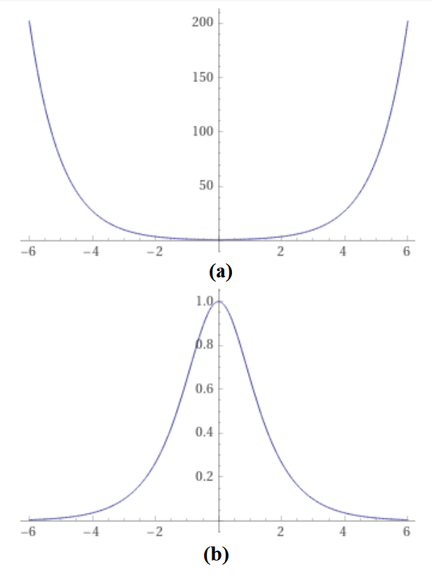
Figure 1: (a) $\text{cosh}(x)$ (b) $1/\text{cosh}(x)$

This function resembles a probability density function (pdf) but in order to satisfy the necessary conditions, it must be non-negative and integrate to 1. The first requirement is already satisfied by inspection. For the second requirement, if we take the integral of the function, we obtain the normalizing constant as

$$\int_{-\infty}^{\infty}\frac{1}{\cosh(x)}dx=\pi.$$

Therefore, the pdf of the Cosh distribution is given by

$$f(x)=\frac{1}{\pi\,\cosh(x)}$$ (4)

The corresponding cumulative distribution function (cdf) is given by:

$$F(x)=\frac{1}{2}+\frac{1}{\pi}{\text{tan}^{-1}\big{[}\sinh\big{(}{x}\big{)}}\big{]}$$ (5)

which is invertible. The cdf and pdf are plotted in Fig. 2.

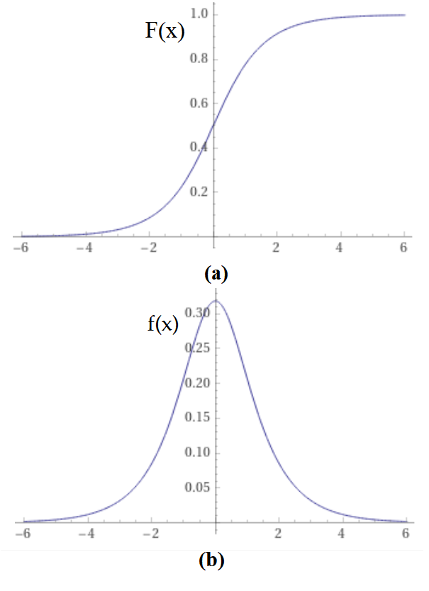
Figure 2: Cosh distribution (a) cdf (b) pdf

More generally, we have a location-scale family of distributions of the form

$$f(x;\theta,\sigma)=\frac{1}{\pi\sigma\,\text{cosh}(\frac{x-\theta}{\sigma})}$$ (6)

where $\theta$ is the location parameter and $\sigma$ is the scale parameter. We note here that

$$\mathbb{E}[X]=\theta\,\,\,\,\,\text{and}\,\,\,\,\,\mathbb{E}[X^{2}]=\frac{\pi^{2}\sigma^{2}}{4}+\theta^{2}$$

so the asymptotic variance is

$$\text{Var}(X)=\mathbb{E}[X^{2}]-\mathbb{E}[X]^{2}=\frac{\pi^{2}\sigma^{2}}{4}.$$

The cdf given by:

$$F(x;\theta,\sigma)=\frac{1}{2}+\frac{1}{\pi}\tan^{-1}\bigg{[}\sinh\bigg{(}\frac{x-\theta}{\sigma}\bigg{)}\bigg{]}.$$ (7)

III-C Maximum Likelihood Estimation

We next develop the maximum likelihood estimator (MLE) for the case of $\sigma=1$, as follows. If $x_{1},x_{2},...,x_{n}$ are i.i.d random variables, then the likelihood function is given by:

$$L(x_{1},x_{2},...,x_{n};\theta)=\prod_{i=1}^{n}\frac{1}{\pi\,\text{cosh}(x_{i}-\theta)}.$$ (8)

The negative log-likelihood expression is given by:

$$-\ell(x_{1},x_{2},...,x_{n};\theta)=n\,\text{log}\pi+\sum_{i=1}^{n}\text{log}(\text{cosh}(x_{i}-\theta)).$$ (9)

The estimator $\hat{\theta}$ is the solution to the equation:

$$\sum_{i=1}^{n}\tanh(x_{i}-\theta)=0$$ (10)

or equivalently

$$\hat{\theta}=\text{argmin}_{\theta\in\mathbb{R}}\sum_{i=1}^{n}\text{log(cosh}(x_{i}-\theta)).$$ (11)

We see that this estimator is, in fact, the MLE of the Cosh distribution. The equation can be solved in a straight-forward manner using a convex optimization procedure due to the fact that it is globally convex. That is, the second derivative can be shown to be non-negative. This can be demonstrated by noting that

$$\psi_{L}(x)=\rho_{L}^{\prime}(x)=\tanh(x)$$ (12)

and

$$\psi_{L}^{\prime}(x)=\rho_{L}^{\prime\prime}(x)=\text{sech}^{2}(x).$$ (13)

Therefore, both the gradient and Hessian terms can be easily obtained and this is important for machine learning applications.

IV An Intuitive View of log-cosh

It is useful to consider the log-cosh loss function from an intuitive standpoint to understand its relative importance. We first examine the loss function in terms of its behavior relative to the L1 and L2 functions. Consider M-estimators of the form

$$\hat{\theta}=\text{argmin}_{\theta\in\mathbb{R}}\frac{1}{n}\sum_{i=1}^{n}\rho(x_{i},\theta).$$ (14)

For example, we can define $\rho(x)$ in any manner we choose such as

$$\rho_{L2}(x)=x^{2}$$ (15)

for least squares estimate (LSE), also called the L2 loss function, and

$$\rho_{L1}(x,\theta)=|x|$$ (16)

for least absolute deviation (LAD), also called the L1 loss function. For log-cosh, we already derived the MLE to be

$$\rho_{L}(x)=\text{log}(\text{cosh}(x))$$ (17)

Next, we compare the log-cosh loss function relative to the L1 and L2 cases above. As $x\rightarrow+\infty$, the log-cosh loss tends towards

$$\text{log(cosh}(x))\approx x-\text{log}(2)$$ (18)

and as $x\rightarrow-\infty$, the function tends towards

$$\text{log(cosh}(x))\approx-x-\text{log}(2).$$ (19)

Therefore, far from $x=0$, the function behaves as

$$\text{log(cosh}(x))\approx|x|-\text{log}(2)$$ (20)

which is like L1 except for the constant term. Now, as $x\rightarrow 0$, we can take a Taylor series expansion at $x=0$ as follows

$$\text{log(cosh}(x))=\frac{x^{2}}{2}-\frac{x^{4}}{12}+\frac{x^{6}}{45}+O(x^{8})$$ (21)

and therefore it is, to first-order, like L2. That is,

$$\text{log(cosh}(x))\approx\frac{x^{2}}{2}$$ (22)

for small $x$. Since it behaves like L2 close to the origin and L1 far from the origin, one can view it as a smoothed out L1 using L2 around the origin. Hence, both the Jacobian and Hessian matrix terms exist for this loss function. For robust regression, this function can be used as an alternative to L1.

Huber [13] proposed a method of combining the best of L1 and L2 by explicitly using L2 in the vicinity of the origin where the discontinuity lies, and then switching to L1 a certain distance, $\delta$, away from the origin. The small interval around the origin is defined by $[-\delta,+\delta]$. Inside this region, the L2 loss function is used since it is continuous. Outside this region, the L1 loss is used but great care is taken to match the derivatives at the interface between the two regions. The resulting Huber loss function is given by:

$$\hat{\theta}_{n}^{\rm H}=\text{argmin}_{\theta}\sum_{i=1}^{n}\rho_{H}(x_{i}-\theta)$$ (23)

where

$$\rho_{H}(x)=\begin{cases}x^{2}/2&\quad\text{if }|x|\leq\delta\\ \delta(|x|-\frac{\delta}{2})&\quad\text{if }|x|>\delta\end{cases}$$ (24)

The derivative of the Huber function is given by:

$$\psi_{H}(x)=\begin{cases}x&\quad\text{if }|x|\leq\delta\\ +\delta&\quad\text{if }x>+\delta\\ -\delta&\quad\text{if }x<-\delta\end{cases}$$ (25)

There are a total of 3 regions defined by the Huber function: $x<-\delta$, $x>+\delta$, and $|x|<\delta$. As shown in Figure 3, the Huber function and its first derivative are both continuous in all regions. In this case, $\delta=1$ for illustrative purposes. However, the second derivative (not shown) is discontinuous. It is clear that $\rho_{H}^{\prime\prime}(x)$ will be discontinuous at both $-\delta$ and $+\delta$. Hence, the Hessian is not defined at those points.

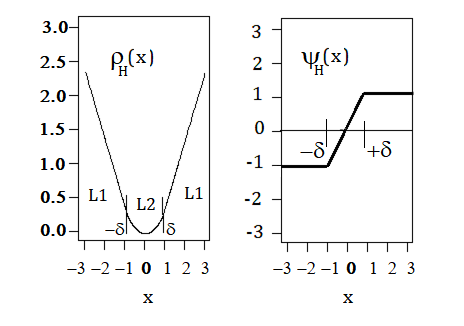
Figure 3: Huber loss and derivative as a function of $x$ for $\delta=1$.

Another intuitive view of log-cosh can be obtained by starting with the L1 loss function. This loss function produces the median as the estimate but it has a discontinuous first derivative. We seek to find a way to construct a continuous function that has continuous first and second derivatives to replace the L1 function. Consider how one might do this intuitively starting with the L1 loss function. This is shown in Fig. 4. The absolute value function, $|x|$, has a “V” shape. When we take its derivative, we obtain sgn($x$) which is discontinuous at $x=0$. We can replace the discontinuous derivative function with a continuous version using $\tanh(x)$. They look about the same but we know that one is discontinuous and the other is continuous. Then, by integrating the $\tanh(x)$ function, we obtain $\log(\cosh(x))$ which does not have a kink (although it may appear to have one in the figure).

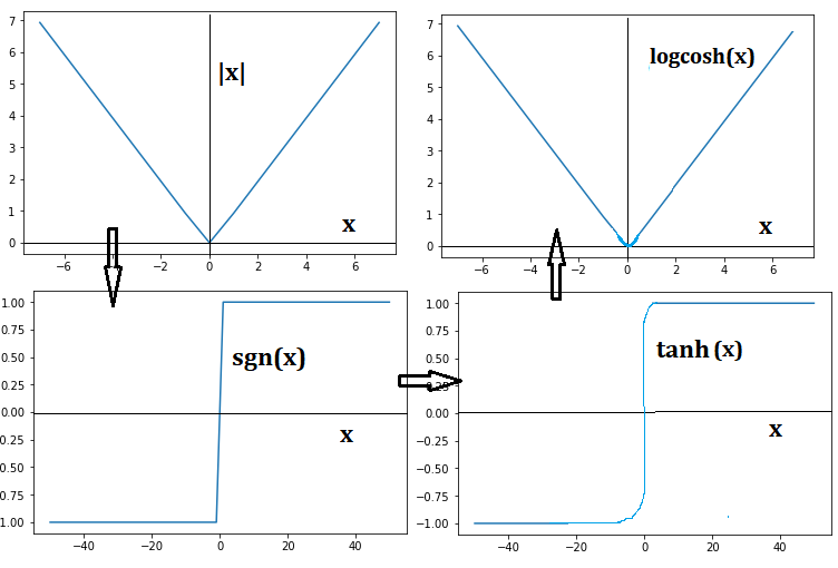
Figure 4: Developing a continuous L1 function.

V Statistical Properties

Consider the general form of the Cosh distribution of Eqn. (6). The MLE of $\theta$ can be derived as given in Eqn. (11). The estimator is represented as $\hat{\theta}$. Then, as $n\rightarrow\infty$, we find that

$$\sqrt{n}(\hat{\theta}-\theta)\overset{\mathcal{D}}{\to}\mathcal{N}(0,\mathcal{I}^{-1}(\theta))$$ (26)

where $\mathcal{I}(\theta)$ is the Fisher information which can be derived as

$$\mathcal{I}(\theta)=\frac{1}{2\sigma^{2}}.$$ (27)

Furthermore, the MLE estimator is consistent such that

$$\hat{\theta}\overset{\mathcal{P}}{\to}\theta$$ (28)

with variance

$$\text{Var}(\hat{\theta})=\frac{1}{n\mathcal{I}(\theta)}.$$

Hence, we find the asymptotic variance of $\hat{\theta}$ to be

$$\text{Var}(\hat{\theta})=\frac{2\sigma^{2}}{n}.$$ (29)

Next, given that $\hat{\theta}\overset{\mathcal{P}}{\to}\theta$, the asymptotic bias is

$$\text{bias}=\mathbb{E}[\hat{\theta}]-\theta=0.$$

The log-cosh estimator is therefore asymptotically unbiased. Further, the $(1-\alpha)$ confidence interval is given by

$$CI=\bigg{[}\hat{\theta}-\frac{z_{\alpha/2}}{\sqrt{n\mathcal{I}(\theta)}},\,\,\hat{\theta}+\frac{z_{\alpha/2}}{\sqrt{n\mathcal{I}(\theta)}}\bigg{]}.$$

We can use the bootstrap method to validate the results. Specifically, we select a sample of size $n$ from a uniform distribution $\mathcal{U}[0,1]$, say $(u_{1},u_{2},...,u_{n})$, to produce the set $x_{i}=F^{-1}(u_{i})$, where $F(x)$ is defined in Eqn. (7). Its inverse is given by

$$F^{-1}(u)=\sigma\,\sinh^{-1}(\text{tan}\big{[}(u-\frac{1}{2})\pi\big{]})+\theta.$$ (30)

The bootstrapped distributions generated in this manner are shown in Fig. 5. A number of different combinations of $\theta$ and $\sigma$ were selected. For each case, estimates of the location parameter, $\hat{\theta}$, and the variance term, $n\widehat{\text{Var}}(\hat{\theta})$, are obtained and listed in the figure. The same results are also provided in Table I along with the estimate of $\hat{\sigma}$. The estimates in all cases validate the equations derived earlier (see Eqn. (29)).

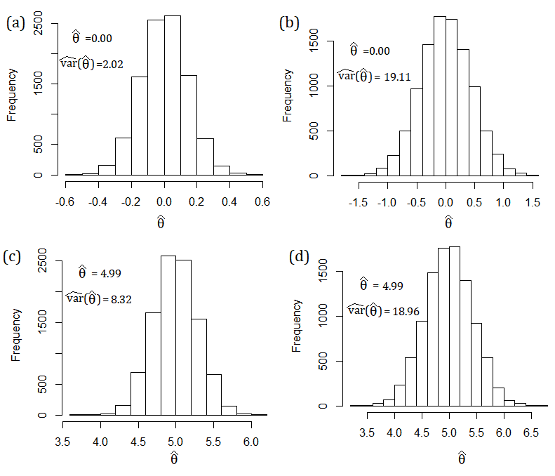
Figure 5: Histogram of estimates of $\hat{\theta}$ and $n\widehat{\text{Var}}(\hat{\theta})$ from 10000 samples with $n=100$.

TABLE I: Location and Variance estimates using bootstrapping.

	Location/Variance
Plot
label	$\theta$	$\sigma$	$\hat{\theta}$	$n\widehat{\text{Var}}(\hat{\theta})$	$\hat{\sigma}$
(a)	0.0	1.0	0.00	2.02	1.00
(b)	0.0	3.0	0.00	19.11	3.09
(c)	5.0	2.0	4.99	8.32	2.04
(d)	5.0	3.0	4.99	18.96	3.08

VI Comparison with Other Distributions

Our next step is to compare the Cosh distribution with the Normal and Cauchy distributions. We begin with a comparison with the standard Normal case. We see in Fig. 6 that the Cosh distribution has heavier tails than the Gaussian $\mathcal{N}(0,1)$ distribution. This is also illustrated in the Q-Q plot of Fig. 7 for a random set of points from the Cosh distribution.

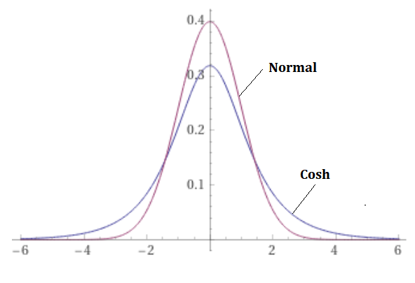
Figure 6: Comparison of standard Normal distribution with Cosh distribution.

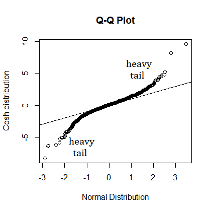
Figure 7: Q-Q plot of Cosh against Normal distribution.

The second comparison is with the Cauchy distribution. One may recognize the form of the pdf of the Cosh distribution as being similar to the Cauchy distribution (Student t distribution with df=1) given by:

$$f(x;\theta,\sigma)=\frac{1}{\pi\sigma\,(1+(\frac{x-\theta)}{\sigma})^{2})}$$ (31)

with corresponding cdf given by

$$F(x;\theta,\sigma)=\frac{1}{2}+\frac{1}{\pi}{\tan^{-1}\bigg{(}\frac{x-\theta}{\sigma}\bigg{)}}.$$ (32)

We note here that for the Cauchy distribution

$$\mathbb{E}[X]=\text{undefined}$$

and

$$\text{Var}(X)=\text{undefined}.$$

This may be one of the reasons why the Cauchy distribution is not used in practice. A graphical comparison of the Cosh and Cauchy distributions is provided in Fig. 8.

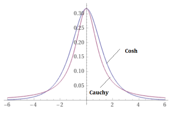
Figure 8: Comparison of Cauchy distribution with Cosh distribution.

We can still develop an estimator based on the Cauchy distribution. Applying MLE produces the following estimator:

$$\hat{\theta}=\text{argmin}_{\theta\in\mathbb{R}}\sum_{i=1}^{n}\text{log}(1+(x_{i}-\theta)^{2})$$ (33)

The associated loss function can be shown to be non-convex so it is not suitable for regression. However, there are simple cases for which it will produce an acceptable result.

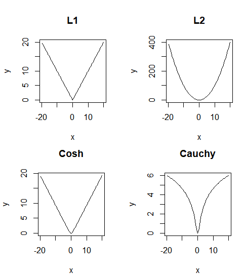
Figure 9: $\rho(x)$ functions.

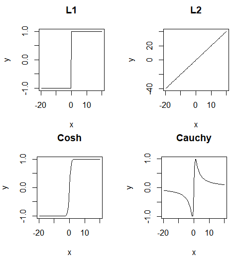
Figure 10: $\psi(x)$ functions.

Figs. 9 and 10 show the characteristics of the $\rho(x)$ and $\psi(x)$ functions derived from the double exponential (L1), Gaussian (L2), Cosh and Cauchy distributions. Comparing the different graphs, it is clear that the Cosh characteristics are very similar to the L1 characteristics. It inherits some of the good properties of L1 without the discontinuities in the first derivative. This is the main reason for its recent rise in popularity in the machine learning community.

VII Regression Examples

VII-A Location Problem

Consider a location problem of the form:

$$y_{i}=\theta+\epsilon_{i},\quad i=1,\ldots,n.$$

The one-dimensional data set under consideration, ranging from -2.8 to 20.5, is given in Table II. For this set, the LS, Cauchy and log-cosh estimates for $\theta$ were computed.

TABLE II: Location problem data set.

(1)	-2.80	-1.98	-1.70	-1.20	-1.10	-0.82
(7)	-0.79	-0.73	-0.66	-0.51	-0.41	-0.35
(13)	-0.23	0.10	0.22	0.25	0.37	0.52
(19)	0.93	0.95	1.36	1.52	1.76	3.07
(25)	20.50	-	-	-	-	-

The results are provided in Table III and illustrated graphically in Fig. 11. We see that the estimates of Cauchy and log-cosh are quite close in value whereas the LSE is much further away due to the outlier on the right-hand side. Asymptotically, the Cauchy estimator should produce the median, which in this case is -0.23 while the mean is 0.73. We also note the standard errors (s.e.’s), obtained using bootstrapping and given in Table III, indicate a 3 times larger value for LSE compared to the relatively smaller values for Cauchy and log-cosh.

TABLE III: Comparison of LSE, Cosh and Cauchy for location problem $n=25$.

Statistic	Technique Used
Used	LSE	Cosh	Cauchy
$\hat{\theta}$	0.73	-0.06	-0.19
s.e.($\hat{\theta}$)	0.84	0.28	0.28

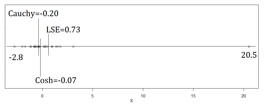
Figure 11: Estimates for Cauchy, Cosh and LSE on location problem.

VII-B Simple Linear Regression Example

We will now compare a number of different methods on a simple linear example from the telephone data set in the Rfit package [14] in R. Rfit uses another robust method called rank-based regression [15] [16] to be described shortly. For our purposes, we will use the Belgium telephone data set [14][15]. This data set is provided in Table IV and contains the number of calls (in units of 10’s of millions) made in Belgium in the years between 1950 - 1973. It has $24$ data points, with $6$ outliers. The outliers are due to a change in measurement technique without re-calibration for $6$ years, as is often cited.

TABLE IV: Belgium telephone data set.

x	1950	1951	1952	1953	1954	1955	1956	1957
y	0.44	0.47	0.47	0.59	0.66	9.73	0.81	0.88
x	1958	1959	1960	1961	1962	1963	1964	1965
y	1.06	1.2	1.35	1.49	1.61	2.12	11.9	12.4
x	1966	1967	1968	1969	1970	1971	1972	1973
y	14.2	15.9	18.2	21.2	4.3	2.4	2.7	2.9

Rank-based methods [15][16] also offer robust regression so it is useful to compare log-cosh against this approach. The rank-based loss function is governed by:

$$\text{loss}_{R}(\beta)=\sum_{i=1}^{n}(y_{i}-x_{i}\beta)a_{n}(R_{n_{i}}(\beta))$$ (34)

where $R_{n_{i}}(\beta)$ are the ranks of the residuals $r_{i}=y_{i}-x_{i}\beta$ and

$$a_{n}(R_{n_{i}}(\beta))=\phi\left(\frac{R_{n_{i}}(\beta)}{n+1}\right)$$ (35)

with $\phi(u)=2u-1$. Further details of these quantities may be found in [15][16].

The results of the regression for LS, Huber, log-cosh, and rank are shown in Fig. 12. The estimates are given in Table V. We note that log-cosh, Huber and rank are all aligned whereas the LSE model is greatly affected by the outliers. This example clearly illustrates the robustness property of the log-cosh estimator. In addition, the Huber and rank results are very similar in this case, while the log-cosh method produces a slightly higher slope. This will vary from dataset to dataset.

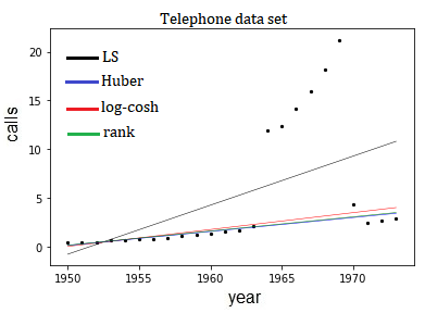
Figure 12: Results for LSE, log-cosh, rank and Huber on a simple linear problem.

TABLE V: Slope and intercept for 4 regression methods on telephone data set.

	$\beta_{1}$	$\beta_{0}$
least squares	0.504	-983.9
log-cosh	0.173	-338.1
rank-based	0.146	-284.3
Huber ($\delta=0.1$)	0.143	-280.0

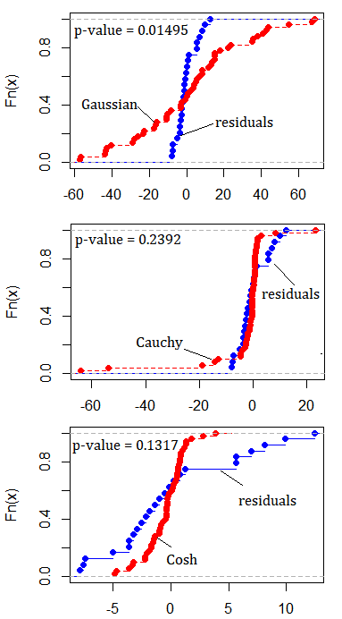
Figure 13: Komlogorov-Smirnov Goodness-of-Fit Test using residuals of Telephone data set comparing p-values of Gaussian, Cauchy and Cosh distributions.

A Goodness-of-fit test can be performed using the Komlogorov-Smirov (K-S) method to examine what distribution best fits the residuals of the telephone data set following least squares estimation (LSE). This test uses the empirical cdf of the distributions. The results are shown graphically in Fig. 13 along with their p-values. We note that the null hypothesis is rejected in the case of the Gaussian distribution at the $\alpha=0.05$ level whereas it cannot be rejected for the Cauchy or Cosh distributions. Hence, one should use a robust method. If the null hypothesis fails, one should consider a robust method. On the other hand, the log-cosh loss provides equivalent estimates in cases when outliers are not present in the data set. Therefore, it may be used whether or not outliers exist.

VIII Multiple Linear Regression

The different approaches for robust regression can be compared in the context of multiple linear regression to study standard errors of the estimates. We use a well-known Swiss Fertility data set with $p=5$ variables and $n=47$ observations. This data set is part of the R environment. The data itself may also be found in [15]. The variable abbreviations are as follows: A = Agriculture, Ex = Examination, Ed = Education, C = Catholic, IM = Infant Mortality. The goal is to build a model that predicts Fertility based on these five explanatory variables. In Table VI, we provide the estimates for Huber (”MASS” in R), Rank (”Rfit” in R) and log-cosh, along with their associated standard errors (s.e.). For the log-cosh method, the s.e.’s were obtained based on [17] as follows. First obtain

$$\hat{v}^{2}=\hat{\sigma}^{2}\frac{\frac{1}{n}\sum\psi_{L}(r_{i}/\hat{\sigma})^{2}}{[\frac{1}{n}\sum\psi_{L}^{\prime}(r_{i}/\hat{\sigma})]^{2}}\frac{n}{n-p}$$ (36)

where $\psi_{L}(x)$ and $\psi_{L}^{\prime}(x)$ are defined in Eqns. (12) and (13), respectively, with residuals $r_{i}=y_{i}-\textbf{x}_{i}^{T}\boldsymbol{\beta}$, and

$$\hat{\sigma}^{2}=\frac{1}{n-p}\sum_{i=1}^{n}r_{i}^{2}.$$ (37)

For large $n$, we treat the estimates as normal with

$$\boldsymbol{\hat{\beta}_{n}^{L}}\sim\mathcal{N}_{p}(\boldsymbol{\beta^{L}},\hat{v}^{2}(\textbf{X}^{T}\textbf{X})^{-1}).$$ (38)

The s.e.’s are computed as the square root of the diagonal elements of the covariance matrix. As seen in Table VI, they all produce similar s.e. values, although the results may vary slightly from dataset to dataset.

TABLE VI: Estimates and standard errors $(s.e.)$ for Huber (H), Rank (R) and log-cosh (L) on Swiss data set.

	$\hat{\beta}_{n}^{H}$	s.e.($\hat{\beta}_{n}^{H}$)	$\hat{\beta}_{n}^{R}$	s.e.($\hat{\beta}_{n}^{R}$)	$\hat{\beta}_{n}^{L}$	s.e.($\hat{\beta}_{n}^{L}$)
A	-0.19	0.071	-0.20	0.069	-0.20	0.069
Ex	-0.28	0.258	-0.25	0.249	-0.26	0.242
Ed	-0.84	0.186	-0.88	0.179	-0.89	0.179
C	0.10	0.035	0.10	0.034	0.10	0.034
IM	1.21	0.388	1.19	0.375	1.40	0.374

IX Quantile Regression

Quantile regression is a robust method for studying the effect of explanatory variables on the entire conditional distribution of the response variable rather than just on the median. It has been used extensively since the initial concepts were developed in the late 1970’s and early 1980’s [18]. It is based on the so-called check function whereby the quantile of interest is set by a parameter, $\tau$. The original check function exhibits a non-monotonic behavior which has been the subject of a number of research papers over the years [20][21][22][23][24]. In [12], we used the log-cosh function to develop a new M-estimator to overcome the crossing problem. In this section, we derive an MLE equivalent so that a statistical analysis can be carried out.

The original check function can be written concisely as follows:

$$\rho_{\tau}(x_{i},\tau)=\begin{cases}-(1-\tau)x_{i}&\quad\text{if }x_{i}<0\\ \tau x_{i}&\quad\text{if }x_{i}\geq 0\end{cases}$$ (39)

where the parameter $\tau\in(0,1)$ is the quantile and $x_{i}$ is the $i$th residual. Different regression quantiles represented by lines or hyperplanes are obtained by selecting $\tau$ and minimizing the conditional quantile function

$$Q_{\tau}(Y|x,\tau)=\sum_{i=1}^{n}\rho_{\tau}(x_{i},\tau).$$ (40)

A plot of $\rho_{\tau}(x_{i},\tau)$ for different values of $\tau$ is provided in Fig. 14. Suppose we are interested in the median, which is also the 50th percentile and the 2nd quartile.

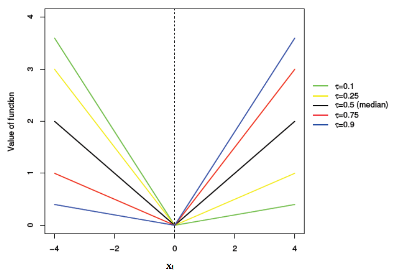
Figure 14: Check function.

We would set $\tau=0.5$ and use the following check function,

$$\rho_{\tau}(x_{i},0.5)=\begin{cases}-(0.5)x_{i}&\quad\text{if }x_{i}<0\\ 0.5x_{i}&\quad\text{if }x_{i}\geq 0.\end{cases}$$ (41)

This is equivalent to the least absolute deviation (LAD) function or the L1 loss function. We see from the figure (black line, $\tau=0.5$) that it is symmetric about $x_{i}=0$ but has a kink at 0. This is the same characteristic that causes problems for the L1 function. Because of this kink, the derivative of this function is discontinuous at 0. Other cases shown in the figure for $\tau=0.1,0.25,0.75,0.9$ all exhibit a kink except that the function is asymmetric in one direction or the other. The red lines associated with $\tau=0.75$ are reminiscent of a check mark, and hence the name check function. In any case, the kinks in this function imply discontinuous derivatives leading to a number of mathematical and numerical problems when solving for quantiles.

IX-A Continuous Check Function

To circumvent this problem, one could employ a continuous check function using log-cosh as follows,

$$\rho_{S}(x,\tau)=\text{log}(\text{cosh}(x))+(\tau-\frac{1}{2})x$$ (42)

This function does not have any kinks as will be demonstrated shortly, but we can already anticipate that it will be smoother simply due to the characteristics of log-cosh.

The quantile regression problem involves minimizing an associated convex loss function which is the conditional quantile function for each $\tau$ given by

$$Q_{S}(Y|x,\tau)=\sum_{i=1}^{n}\rho_{S}(r_{i},\tau).$$ (43)

To derive this continuous check function, we first postulate a pdf given by

$$f(x)=\frac{e^{-(\tau-\frac{1}{2})x}}{\kappa\,\text{cosh}(x)}$$ (44)

where $\kappa$ is a normalizing constant term such that the pdf integrates to 1. The value of $\kappa$ will vary as a function of the selected $\tau$. A table of values for $\kappa$ for selected $\tau$ values is given in Table VII. Note that for $\tau=0.5$, we obtain that $\kappa=\pi$ as expected, since it is the original log-cosh pdf.

TABLE VII: Selected values of $\kappa$

$\tau$	$\kappa$
0.0	$\pi\sqrt{2}$
0.25	$\pi\sqrt{4-2\sqrt{2}}$
0.5	$\pi$
0.75	$\pi\sqrt{4-2\sqrt{2}}$
1.0	$\pi\sqrt{2}$

The MLE for this distribution can be derived as follows:

$$L(x_{1},...,x_{n})=\bigg{(}\frac{e^{-(\tau-\frac{1}{2})x_{1}}}{\kappa\,\text{cosh}(x_{1})}\bigg{)}\dots\bigg{(}\frac{e^{-(\tau-\frac{1}{2})x_{n}}}{\kappa\,\text{cosh}(x_{n})}\bigg{)}.$$ (45)

Then,

$$-\ell(x_{1},...,x_{n})=\sum_{i=1}^{n}[\text{log(cosh}(x_{i}))+(\tau-\frac{1}{2})x_{i}+\text{log}(\kappa)]$$ (46)

Therefore, after removing the constant term, we obtain Eqns. (42) and (43). The Fisher information can be derived to be

$$\mathcal{I}(\theta)=\frac{1}{2}.$$ (47)

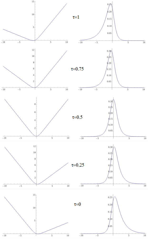
Figure 15: pdf of quantile function.

The distributions and loss functions can now be plotted. Starting with Eqn. (44) and the normalizing constants $\kappa$ given in Table VII, different values of $\tau$ were selected and their associated distributions plotted in Fig. 15. The cases shown are for $\tau=0,0.25,0.5,0.75,1.0$. The distributions shown on the right-hand side of the figure can be seen to skew from one side to the other as $\tau$ decreases in value from 1 to 0. On the left-hand side, we have plotted the loss term of the MLE in each case. We see that the use of the logcosh function smooths out the kinks of the original loss function (see Fig. 14).

A more general M-estimator based on log-cosh for quantile regression is given by:

$$\rho_{SMRQ}(x,\tau)=\frac{1}{2c}\text{log}(\text{cosh}(c(x-h)))+(\tau-s)x+v$$ (48)

where $c$ is the desired curvature of the function (i.e. the severity of the kink), $v$ controls vertical shift, $h$ controls the horizontal shift and $\tau-s$ is used to produce the asymptotic slopes on the two sides of the check function itself.

Quantile regression using the above equation is referred to as SMRQ for ‘smoother regression quantiles’. Fig. 16 shows five different cases of Eqn. (48) by varying parameters $c$ and $v$ (while holding $s=0.5$ and $h=0$ fixed) for $\tau=0.5$ and $\tau=0.7$. One can observe the different levels of smoothness offered by the flexible check function, which can be varied easily as the need arises.

We propose the use of $c=1/2$ and $v=1/2$ to produce:

$$\rho_{SMRQ}(x,\tau)=\text{log}(\text{cosh}\big{(}\frac{x}{2}\big{)})+(\tau-\frac{1}{2})x+\frac{1}{2}.$$ (49)

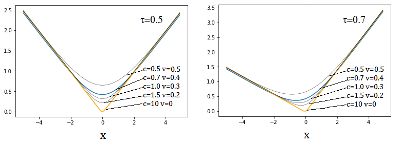
Figure 16: Loss functions for SMRQ for $\tau=0.5$ and $\tau=0.7$ cases.

The variance of the estimates due to this loss function cannot be obtained in closed form. Therefore, a bootstrapping method can be used to extract standard errors for estimates, which are naturally related to the variance.

IX-B Comparison with Convolutional Smoothing

Recently, a technique was published [25] that utilizes convolutional smoothing [26] applied to the loss function and is implemented in the conquer library in R. Convolutional smoothing provides a different approach to reducing the crossing problem. Therefore, it is appropriate to compare it with SMRQ in terms of solving the crossing problem.

One natural way to monitor the monotonicity of a quantile regression method is to simply count the number of data points below a given regression line (or hyperplane in the multivariate case). The median line (50th percentile) should result in half the points below it. The 75th percentile should results in 75% of the data below that line, and so on. One rule that should be enforced is that a higher percentile will have more points below it than a lower percentile. That is, we should not have more points below the 75th percentile than we do at the 80th percentile. This would violate the basic definition of percentiles, which is not desirable. However, in the original formulation of quantile regression [19], this was often the case and was called the quantile crossing problem.

To investigate the monotonicity of conquer and SMRQ, we selected the well-known swiss data set in R, which has 5 variables. We show the monotonicity results for conquer and SMRQ in Fig. 17. Note that the plot should be non-decreasing if the crossing problem is avoided. This is true for SMRQ but conquer exhibits 1 non-monotonic event.

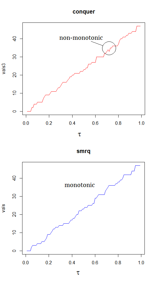
Figure 17: Conquer vs. SMRQ on the swiss data set.

We now compare the standard errors (s.e.) of conquer and SMRQ in Table VIII. Rather than listing each s.e. for all 5 variables in the 5 cases of $\tau$ (total of 25 values each), we compute the $L_{2}$-norm of the s.e.’s and list those values in the table. The numbers represent an aggregate standard error for each $\tau$ which is sufficient for this comparison.

We see that the errors are on average 10% smaller for SMRQ compared to conquer. A similar result was also obtained on the diabetes dataset in R. In addition, SMRQ possesses the monotonocity property for quartiles, deciles and percentiles whereas conquer may exhibit some non-monotonic behavior. However, conquer was intended to handle large-scale problems and requires less runtime for the same size problem. This is a relatively small example for conquer, but it is expected to perform much better with large data sets.

TABLE VIII: s.e. for conquest and SMRQ as a function of $\tau$ on swiss data set.

Quantile	conquer (C)	SMRQ (S)
$\tau$	$||(s.e._{C})||_{2}$	$||(s.e._{S})||_{2}$
0.01	0.851	0.781
0.25	0.781	0.792
0.5	0.755	0.710
0.75	0.921	0.756
0.99	0.825	0.753

X Conclusions

In this paper, we identified the Cosh distribution from which the MLE for the log-cosh function can be derived. We then derived the asymptotic variance, asymptotic bias and confidence intervals. The log-cosh loss function was compared to the Huber, rank and LSE loss functions in the case of simple linear regression. The estimates and standard errors were found to be similar for Huber, rank and log-cosh for multiple linear regression. Next, the use of log-cosh in quantile regression was described to resolve the crossing problem, the details of which can be found in [12]. The M-estimator for quantile regression was compared and found to have a smaller standard error than conquer, which uses convolutional smoothing. From the analysis provided herein, it is clear that the log-cosh is an important loss function for machine learning and is expected to increase in use over the coming years.

References

- [1] Grover, P. (2019, September 25). “5 Regression Loss Functions All Machine Learners Should Know”. Retrieved from https://heartbeat.fritz.ai/5-regression-loss-functions-all-machine-learners-should-know-4fb140e9d4b0.
- [2] Gupta,S. (2022, April 14). “The 7 Most Common Machine Learning Loss Functions”. Retrieved from https://builtin.com/machine-learning/common-loss-functions.
- [3] Wang, Q. et. al, “A Comprehensive Survey of Loss Functions in Machine Learning”, Annals of Data Science 9, April 2020.
- [4] Jadon, S. “A survey of loss functions for semantic segmentation”, arXiv:2006.14822v4, Sept. 2020.
- [5] R software, limma package.
- [6] numpy documentation, https://numpy.org/doc.
- [7] TensorFlow documentation regarding log-cosh loss, Retrieved from https://www.tensorflow.org/api-docs/python/tf/keras/losses/log-cosh.
- [8] PyTorch documentation, https://pytorch.org/doc.
- [9] Chen P., Chen G., Zhang S. “Log Hyperbolic Cosine Loss Improves Variational Auto-Encoder”, Proceedings of the 2018 Sixth International Conference on Learning Representations, Vancouver, BC, Canada. 30 April–3 May 2018.
- [10] X. Xu, J. Li, Y. Yang and F. Shen, ”Toward Effective Intrusion Detection Using Log-Cosh Conditional Variational Autoencoder,” in IEEE Internet of Things Journal, vol. 8, no. 8, pp. 6187-6196, April 2021.
- [11] Kalifi, E. Y. et. al, “Classification of Breast Cancer Lesions in Ultrasound Images by Using Attention Layer and Loss Ensemble in Deep Convolutional Neural Networks,” National Library of Medicine, published online Oct. 2021.
- [12] Saleh, R., and Saleh, A.K.Md. E., “Solution to the Non-Monotonicity and Crossing Problems in Quantile Regression”, arXiv:2111.04805v2, Nov. 2021.
- [13] Huber, P. J., Ronchetti, E. M., “Robust Statistics”, Second Edition, 2009.
- [14] Kloke, J.D., McKean, J.W., “Rfit:Rank-based estimation for linear models”, The R Journal, 4(2), 57-64, 2012.
- [15] Saleh, A.K.Md.E. et. al, “Rank-based Shrinkage and Selection with Application to Machine Learning”, John Wiley and Sons Publishers, Feb. 2022.
- [16] Hettmansperger, T. P., McKean, J. W., “Robust Nonparametric Statistical Methods”, 2nd Ed. Chapman Hall, New York, 2011.
- [17] Maronna, R.A., Martin, R.D., Yohai, V.J., Salibian-Barrera, M., “Robust Statistics Theory and Method (in R)”, 2nd Edition, John Wiley and Sons Publishers, 2019.
- [18] Koenker, R., and Bassett, “Regression Quantiles,” Econometrica 46, 33-50 (1978).
- [19] Koenker, R., Quantile Regression, Cambridge University Press, 2005.
- [20] He, X., “Quantile Curves without Crossing”, The American Statistician 51, 186-192 (1997).
- [21] Bondell, H.D., B.J. Reich and X. Wang, “Noncrossing quantile regression curve estimation”, Biometrika, 97: 825-838, 2010.
- [22] Amerise, I., “Quantile Regression Estimation Using Non-Crossing Constraints”, Journal of Mathematics and Statistics, Volume 14: 107-118, 2018.
- [23] Neocleous, T. and Portnoy, S. “On Monotonicity of Regression Quantile Functions”, Statistics and Probability Letters, 78: 1226-1229, 2007.
- [24] Chernozhukov, V. and Fernandez-Val, I. and Galichon, A., “ Quantile and probability curves without crossing”, Econometrica 78, 1093-1125, 2010.
- [25] He, X., Pan, X., Tan, K. M., and Zhou, W., “Smoothed Quantile Regression with Large-Scale Inference”, arXiv:202.05187v1, 2020.
- [26] Fernandes, M. and Guerre, E. and Horta, E., “Smoothing quantile regressions”, arXiv:1905.08535v3, Aug. 2019.