Hierarchical Residual Learning Based Vector Quantized Image Modeling with VQVAE

Hierarchical Residual Learning Based Vector Quantized Variational Autoencoder for Image Reconstruction and Generation

Abstract

We propose a multi-layer variational autoencoder method, we call HR-VQVAE, that learns hierarchical discrete representations of the data. By utilizing a novel objective function, each layer in HR-VQVAE learns a discrete representation of the residual from previous layers through a vector quantized encoder. Furthermore, the representations at each layer are hierarchically linked to those at previous layers. We evaluate our method on the tasks of image reconstruction and generation. Experimental results demonstrate that the discrete representations learned by HR-VQVAE enable the decoder to reconstruct high-quality images with less distortion than the baseline methods, namely VQVAE and VQVAE-2. HR-VQVAE can also generate high-quality and diverse images that outperform state-of-the-art generative models, providing further verification of the efficiency of the learned representations. The hierarchical nature of HR-VQVAE i) reduces the decoding search time, making the method particularly suitable for high-load tasks and ii) allows to increase the codebook size without incurring the codebook collapse problem.

1 Introduction

Deep generative modeling has shown impressive results for the application of unsupervised learning in many domains, e.g., image super-resolution [Ledig et al.(2017)Ledig, Theis, Huszár, Caballero, Cunningham, Acosta, Aitken, Tejani, Totz, Wang, et al.], image generation [Theis et al.(2016)Theis, van den Oord, and Bethge], and future video frame prediction [Liang et al.(2017)Liang, Lee, Dai, and Xing]. Variational autoencoders (VAEs) [Zhao et al.(2017)Zhao, Song, and Ermon], which are the focus of this work, compute continuous-valued representations by compressing information into a dense, distributed embedding [Zhao et al.(2017)Zhao, Song, and Ermon]. However, studies on human cognition emphasize the importance of discretization in representation learning. Discrete symbolic representations contribute to reasoning, understanding, generalization, and efficient learning [Cartuyvels et al.(2021)Cartuyvels, Spinks, and Moens]. Discrete representations can also significantly reduce the computational complexity and improve interpretability by illustrating which terms contributed to the solution [Mordatch and Abbeel(2018)].

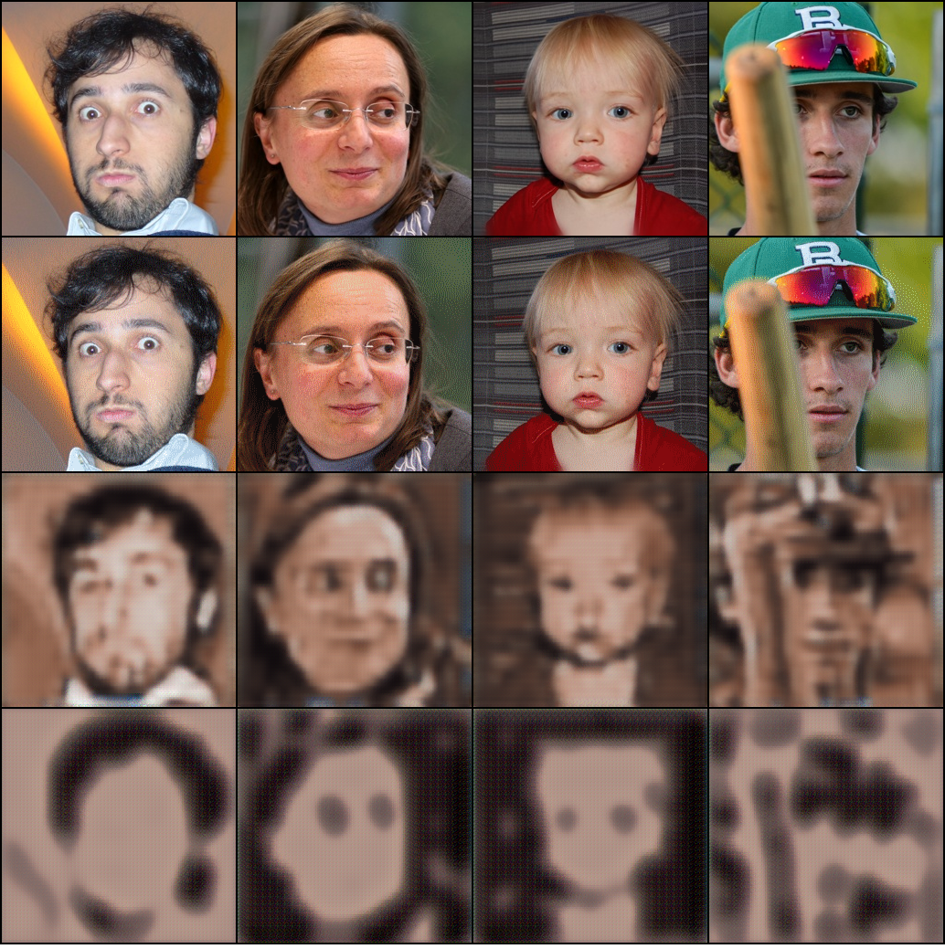
(a) FFHQ

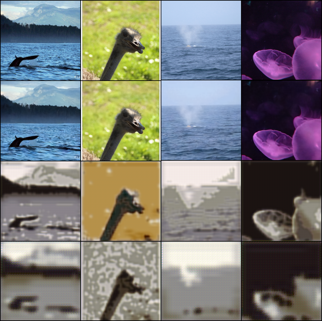
(b) Imagenet

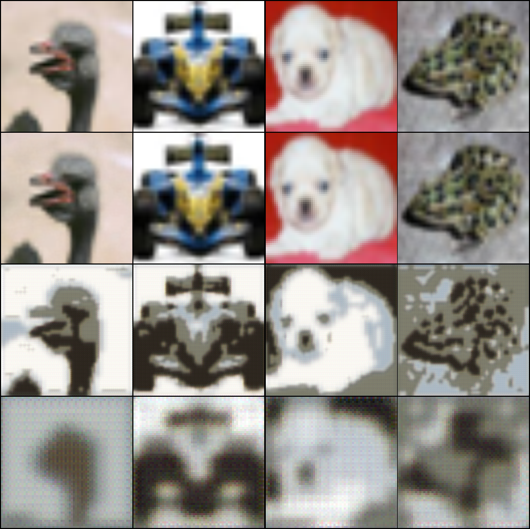
(c) CIFAR10

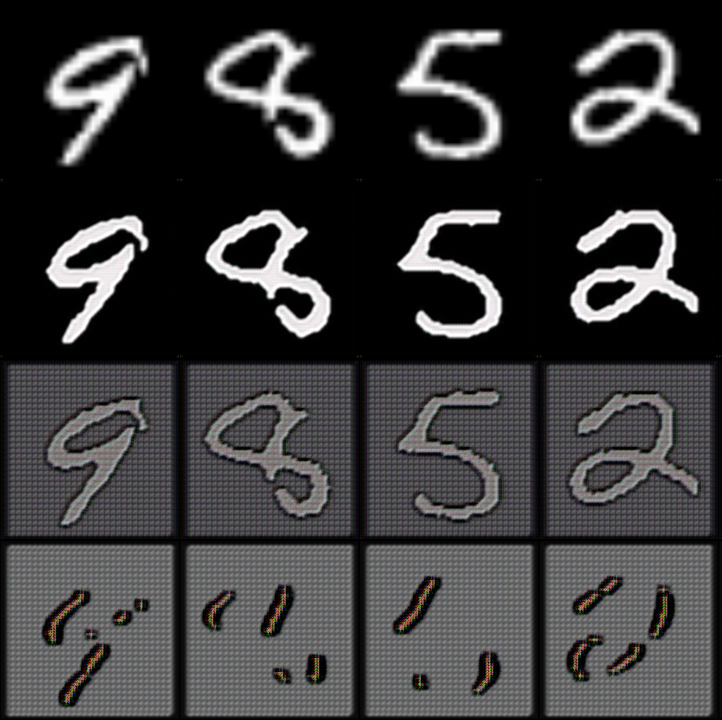
(d) MNIST

Figure 1: Reconstructions obtained with HR-VQVAE. First row contains the original images. Second row contains reconstructions using all three layers. Third row indicates reconstructions using the second and third layers. Last row is the reconstructions using only the third layer. Each layer adds extra details to the final reconstruction.

Rolfe et al. [Rolfe(2016)] proposed a discrete VAE to train a class of probabilistic models with discrete latent variables. By combining undirected discrete component and a directed hierarchical continuous component, the model efficiently learns both the class of objects in an image and their specific realization in pixels in an unsupervised fashion. Oord et al. [van den Oord et al.(2017)van den Oord, Vinyals, et al.] proposed the vector quantized VAE (VQVAE), a discrete latent VAE model that relies on a vector quantization layer to model discrete latent variables, which quantizes encoder outputs with on-line $k$-means clustering. The discrete latent variables allow the use of a powerful autoregressive model that avoids the posterior collapse problem. Moreover, the model can considerably reduce the amount of information required to reconstruct an image. However, VQVAE suffers from the problem of codebook collapse [Dieleman et al.(2018)Dieleman, van den Oord, and Simonyan]: At some point during training, some portion of the codebook may fall out of use and the model no longer uses the full capacity of the discrete representations, resulting in a poor reconstruction [Łańcucki et al.(2020)Łańcucki, Chorowski, Sanchez, Marxer, Chen, Dolfing, Khurana, Alumäe, and Laurent]. One of the explanations of codebook collapse can be found in the typical $k$-means issues [Łańcucki et al.(2020)Łańcucki, Chorowski, Sanchez, Marxer, Chen, Dolfing, Khurana, Alumäe, and Laurent] concerning its sensitivity to initialization and non-stationarity of clustered neural activations during training. Moreover, $k$-means issues become more severe with the increase of centroids, and the ability to encode the input with a broad number of discrete codes decreases [Chorowski et al.(2019)Chorowski, Chen, Marxer, Dolfing, Łańcucki, Sanchez, Alumäe, and Laurent].

More recently, several attempts have been made at introducing hierarchical quantized architectures. In the hierarchical quantized autoencoder [Williams et al.(2020)Williams, Ringer, Ash, Hughes, MacLeod, and Dougherty], low-resolution discrete representations are decoded to match high-resolution representations and again quantized with a stochastic assignment. For example, Takahashi et al. [Takahashi et al.(2021)Takahashi, Singh, and Mitsufuji] proposed a hierarchical representation learning based on VQVAE that enables learning disentangled representations with multiple resolutions independently. Razavi et al. [Razavi et al.(2019)Razavi, van den Oord, and Vinyals] proposed a hierarchical VQVAE, namely VQVAE-2, which extends VQVAE by employing several layers (e.g., top, middle, and bottom layers) of quantized representations to handle hierarchical information in images. Then, two autoregressive convolutional networks [Albawi et al.(2017)Albawi, Mohammed, and Al-Zawi] were used to model structural and textural information, respectively, to generate new images. Different layers, however, share the same objective function. This does not encourage the layers to encode complementary information, and results in inefficient use of the codebooks, as we will show in this paper. Furthermore, VQVAE-2 also suffers from the codebook collapse issue [Zhao et al.(2020)Zhao, Yu, Mahapatra, Su, and Chen, Coppock(2020)].

In this study, we propose a hierarchical residual learning based vector quantized variational autoencoder (HR-VQVAE) for the image reconstruction and generation tasks. The first contribution is a novel hierarchical vector quantization encoding scheme. In contrast with previous research, our scheme maps the continuous latent representations to several layers of discrete representations through hierarchical codebooks. Moreover, a novel objective function is proposed to provide contrastive learning by pushing each layer to extract information not learned by its preceding layers. At the same time, the objective optimizes the output image from the combination of representations obtained from all layers (see Fig. 1). The hierarchical nature of HR-VQVAE allows us to increase the size of the codebooks without incurring in the codebook collapse problem, resulting in higher quality images. It also provides local access to the codebook layers, thus reducing the search time per layer and speeding up the entire search process. With experiments on well-known image datasets, we show that our model can reconstruct images with higher levels of details and is an order of magnitude faster than state-of-the-art methods (i.e., VQVAE [Rolfe(2016)] and VQVAE-2 [Razavi et al.(2019)Razavi, van den Oord, and Vinyals]). Moreover, we show that HR-VQVAE can generate high-quality images that challenge some state-of-the-art approaches (i.e., VDVAE [Child(2020)] and VQGAN [Esser et al.(2021)Esser, Rombach, and Ommer]).

The rest of this work is organized as follows. First, we introduce the background in Section 2. Then, we present the proposed approach in Section 3. Subsequently, experiments and discussion are given in Section 4. Finally, we conclude our work in Section 5.

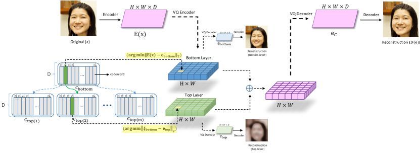
Figure 2: The HR-VQVAE method (only two consecutive layers are shown for simplicity).

2 Background

In this section, we describe aspects of the VQVAE [van den Oord et al.(2017)van den Oord, Vinyals, et al.] and VQVAE-2 [Razavi et al.(2019)Razavi, van den Oord, and Vinyals] models that are necessary to understand the proposed method. VQVAE first encodes the input image $\mathbf{x}\in\mathbb{R}^{{H_{I}\times W_{I}\times 3}}$ into a continuous latent vector $\mathbf{z}=E(\mathbf{x})\in\mathbb{R}^{{H\times W\times D}}$ using a non-linear transformation $E(\cdot)$. Next, each element $\mathbf{z}_{hw}\in\mathbb{R}^{D},h\in[1,H],w\in[1,W]$ in the continuous latent representation $\mathbf{z}$ is quantized to the nearest codebook vector (i.e. codeword) $\mathbf{e}_{k}\in\mathbb{R}^{D},~{}k\in 1,...,m$ by

$$\text{Quantize}(\mathbf{z}_{hw})=\mathbf{e}_{k}\text{ where }k=\arg\min_{j}||\mathbf{z}_{hw}-\mathbf{e}_{j}||_{2},$$ (1)

as illustrated in Fig. 3 (left). The quantized vectors corresponding to each element $\mathbf{z}_{hw}$ are then recombined into the quantized representation $\mathbf{e}\in\mathbb{R}^{{H\times W\times D}}$ to form the input to a decoder that reconstructs the original image through a non-linear function $\mathcal{D(\cdot)}$. The encoder $E(\cdot)$, the codeword $\{\mathbf{e}_{k}\}$, and the decoder $\mathcal{D}(\cdot)$ are learned from data by optimizing the objective function

$$\mathcal{L}(\mathbf{x},\mathcal{D}(\mathbf{e}))=\lVert\mathbf{x}-\mathcal{D}(\mathbf{e})\rVert^{2}_{2}+\lVert\text{sg}[\mathbf{z}]-\mathbf{e}\rVert^{2}_{2}+\beta\lVert\text{sg}[\mathbf{e}]-\mathbf{z}\rVert^{2}_{2}.$$ (2)

This function aims at minimizing the reconstruction error $\lVert\mathbf{x}-\mathcal{D}(\mathbf{e})\rVert_{2}$ whilst minimizing the quantization error $\lVert\mathbf{z}-\mathbf{e}\rVert_{2}$. In Eq. 2, $\text{sg}(.)$ refers to a stop-gradient operator that cuts the gradient flow through its argument during the backpropagation, and $\beta$ is a hyperparameter which controls the reluctance to change the latent representation corresponding to the encoder output.

VQVAE-2 extends VQVAE to attain a hierarchy of vector quantized codes. It compresses images into several latent spaces, from the top layer (smaller size) to the bottom layer (larger size), which is conditioned on the top layer in order for the top layer to extract general information from the image and the bottom layer to add more detail in the image reconstruction. The codebooks at different layers, however, are not related by a hierarchy.

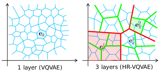
Figure 3: Illustration of vector quantization for 1-layer HR-VQVAE (or VQVAE, left) and 3-layer HR-VQVAE (right). Different colors refer to different layers. For each layer, the Voronoi cell for one centroid is shaded and annotated as an example (See Eq. 1 and 3).

3 Proposed Approach

The architecture of the proposed HR-VQVAE is illustrated in Fig. 2, where we only show two consecutive layers for simplicity. As in VQVAE, the original image $\mathbf{x}$ is first encoded into continuous embeddings that we call $\boldsymbol{\xi}^{0}=E(\mathbf{x})$ by a non-linear encoder. Differently from VQVAE, however, these embeddings are then iteratively quantized into $n$ hierarchical layers of discrete latent variables. Assuming the first layer has a codebook of size $m$, the second layer will have $m$ codebooks of size $m$, and so on for subsequent layers. In general, layer $i$ has $m^{i-1}$ codebooks of size $m$, for a total of $m^{i}$ codewords. However, only one of those codebooks is used in each layer depending on which codewords where chosen in the previous layers. This is illustrated in Fig. 2 where the vector selected within $C_{\text{bottom}}$ determines the codebook that is activated in the top layer (in this case $C_{\text{top}}(2)$). Such a hierarchical searching procedure provides the advantage of local access to codebook indexes, which dramatically reduces search time. Fig. 3 (right) exemplifies this structure where the number of layers $n=3$ and the codebook size $m=4$. The resulting Voronoi cells are shown in red, green and blue for the first, second and third layer, respectively.

In each layer $i$, the codebook is optimized to minimize the error between the codewords $\mathbf{e}^{i}_{k}\in\mathbb{R}^{D}$ and the elements $\boldsymbol{\xi}^{i-1}_{hw}\in\mathbb{R}^{D}$ of the residual error from the previous layer:

$$\text{Quantize}^{i}(\boldsymbol{\xi}^{i-1}_{hw})=\mathbf{e}^{i}_{k}\text{ where }k=\arg\min_{j}\lVert\boldsymbol{\xi}^{i-1}_{hw}-\mathbf{e}^{i}_{j}\rVert_{2},$$ (3)

and $\mathbf{e}_{k}^{i}$ belongs to one of the possible codebooks $C_{i}(t)$ for layer $i$. Which codebook is used is determined by the codeword $\mathbf{e}_{t}^{i-1}$ selected at the previous layer.

Within each layer, the codewords $\mathbf{e}^{i}_{k}$ are combined to form the tensor $\mathbf{e}^{i}\in\mathbb{R}^{{H\times W\times D}}$. Across the different layers, we then combine the tensors $\mathbf{e}^{i}$ to form the “combined” discrete representation $\mathbf{e}_{C}$ which, in turn, is fed into the decoder that reconstructs the image $\mathbf{x}$.

$$\mathbf{e}_{C}=\sum_{i=1}^{n}\mathbf{e}^{i},$$ (4)

By doing this, we allow the combined discrete latent representation $\mathbf{e}_{C}$ to incorporate different aspects of the image, depending on the area that we try to reconstruct. The objective function used to train the system is:

$$\mathcal{L}({\mathbf{x}},\mathcal{D}({\mathbf{e}_{C}}))=\lVert{\mathbf{x}}-\mathcal{D}({\mathbf{e}_{C}})\rVert^{2}_{2}+\lVert\text{sg}[\boldsymbol{\xi}^{0}]-{\mathbf{e}_{C}}\rVert^{2}_{2}+\beta_{0}\lVert\text{sg}[{\mathbf{e}_{C}}]-\boldsymbol{\xi}^{0}\rVert^{2}_{2}+\sum_{i=1}^{n}\mathcal{L}(\boldsymbol{\xi}^{i-1},\mathbf{e^{i}}),$$ (5)

with

$$\mathcal{L}(\boldsymbol{\xi}^{i-1},\mathbf{e^{i}})=\lVert\text{sg}[\boldsymbol{\xi}^{i-1}]-\mathbf{e}^{i}\rVert^{2}_{2}+\beta_{i}\lVert\text{sg}[\mathbf{e}^{i}]-\boldsymbol{\xi}^{i-1}\rVert^{2}_{2},$$ (6)

where $\beta_{i}$ are hyperparameters which control the reluctance to change the code corresponding to the encoder output.

The main goal of Eqs. 5, and 6 is to make a hierarchical mapping of input data in which each layer of quantization extracts residual concepts from its bottom layers. In this regard, $\boldsymbol{\xi}^{i}$ (Eq. 6) plays an essential role in making the hierarchically learning of layers which makes the main differences between our model and the VQVAE-2 model. It should be noted that both VQ encoder and decoder share the same hierarchical codebooks.

Finally, as in VQVAE, for each $\mathbf{e_{C}}$ we fit a prior distribution to all training samples using an autoregressive model (PixelCNN [Van den Oord et al.(2016)Van den Oord, Kalchbrenner, Espeholt, Vinyals, Graves, et al.]). Such a model factorizes the joint probability distribution over the input space into a product of conditional distributions for each dimension of the sample. For generation of new images we use ancestral sampling taking advantage of the chain rule of probability.

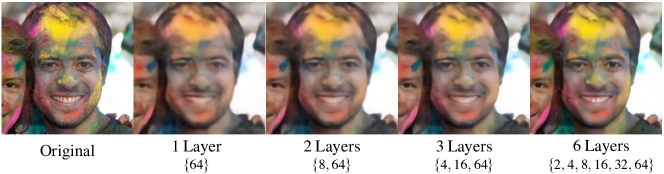
Figure 4: Reconstructions obtained with HR-VQVAE models with different depths (i.e., number of layers). The latent maps are $32\times 32$, and the number of codewords for each layer is specified from bottom to top in order from right to left for each model.

4 Experiments and Discussion

We conducted our experiments on four well-known datasets, FFHQ [Karras et al.(2019)Karras, Laine, and Aila] ($256\times 256$), ImageNet [Deng et al.(2009)Deng, Dong, Socher, Li, Li, and Fei-Fei] ($128\times 128$), CIFAR10 [Krizhevsky et al.(2009)Krizhevsky, Hinton, et al.] ($32\times 32$) and MNIST [LeCun et al.(1998)LeCun, Bottou, Bengio, and Haffner] ($28\times 28$). We start this section by investigating the effect of varying the depth of the hierarchy in our model. To this end, we defined models with $n$ layers and $m$ codewords per codebook. As explained in Sec. 3, the number of codewords in each layer $i$ is $m^{i}$, and, therefore the layers will have $\{m,m^{2},\dots,m^{n}\}$ codewords. To ensure the same level of resolution among the models we compare models with the same number of codewords in the final layer, which corresponds to the maximum resolution. Fig. 4, shows HR-VQVAE reconstructions with different numbers of layers, namely from one to six. Although all configurations have 64 codewords in the final layer, we observe that increasing the depth of the model results in reconstructions with more details (zoom into the pdf version). A possible explanation for such an improvement is that the hierarchical nature of the codebooks acts as regularization during training and allows the model to allocate codewords more efficiently.

Fig. 5 provides a comparison with VQVAE-2 on the effect of the model depth (i.e., number of layers) in terms of the reconstruction mean square error (MSE) [Zhang and Wu(2005)]. The results demonstrate that increasing the model depth leads to better performance of HR-VQVAE compared to VQVAE-2. Furthermore, the performance of HR-VQVAE improves consistently for all datasets with the increase in the number of layers. However, increasing the number of layers does not improve the performance of VQVAE-2 (for Imagenet and FFHQ) from a certain point, and in some cases (MNIST and CIFAR10), the performance decreases. In the following experiments, we will use three layers in HR-VQVAE to be able to compare with VQVAE-2 which also uses three layers, while VQVAE uses a single layer.

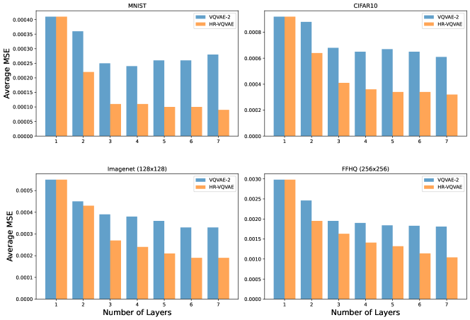
Figure 5: The effect of model depth (number of layers) on image reconstruction.

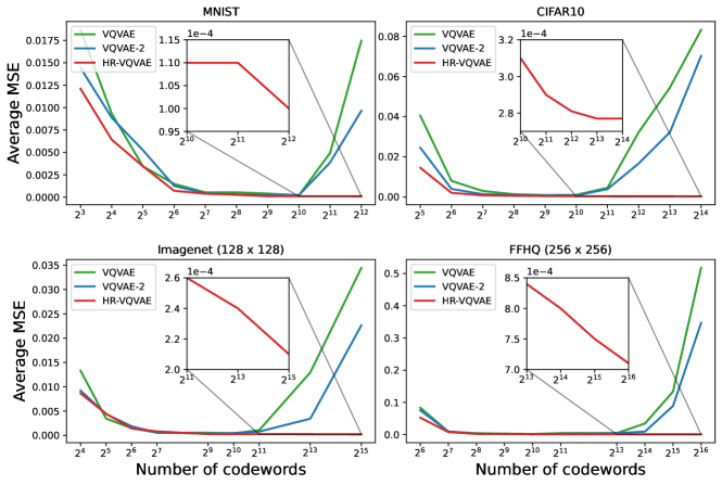
Figure 6: Average MSE vs number of codewords for different datasets and methods. Both VQVAE and VQVAE-2 collapse when the codebook size is increased over a certain limit. However, HR-VQVAE continues improving as shown in the zoom windows inside each plot.

We first compare the effect of increasing the codebook size in our model as well as VQVAE and VQVAE-2. Fig. 6 illustrates the behavior of HR-VQVAE and the baseline models with different numbers of codewords. As it can be seen, by increasing the number of codewords up to a certain number, the performance of all models improves, whereas HR-VQVAE shows higher performance. However, the efficiency of the baseline models starts decreasing from a certain point with increasing the number of codewords, while the efficiency of HR-VQVAE continuously increases for all datasets. This means that not only HR-VQVAE does not suffer from the codebook collapse problem, but it can also benefit from increasing the number of codebooks to improve performance. Fig. 7 provides a visual example for Fig. 6. Fig. 7 (b) shows reconstructions where the size of codebooks is 512 for VQVAE, $\{512,512,512\}$ for VQVAE-2 and $\{8,64,512\}$ for HR-VQVAE. Similarly to Fig. 4, HR-VQVAE produces superior details than VQVAE with the same codebook size (zoom into the pdf version). VQVAE-2 produces a very smooth image but misses some of the details. More interesting is to study what happens if we increase the codebook size in all the models. Fig. 7 (c) shows that both VQVAE and VQVAE-2 are affected by codebook collapse. On the contrary, HR-VQVAE can take full advantage of the increased complexity and produces the best reconstruction of this list.

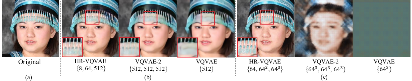
Figure 7: Reconstructions obtained with HR-VQVAE, VQVAE-2 and VQVAE. Number of codewords per layer are given for each model. Both VQVAE and VQVAE-2 are clearly affected by the codebook collapse problem.

Fig. 8 compares 3-layers HR-VQVAE and 3-layer VQVAE-2 to illustrate the different information encoded in different layers in the two models. HR-VQVAE image reconstructions (first row) attain a better reconstruction quality with more details than VQVAE-2 (second row). One possible explanation is that HR-VQVAE encourages the different layers to encode different information about the image; whereas the information in VQVAE-2 is strongly overlapping. This may result in a less efficient latent representation.

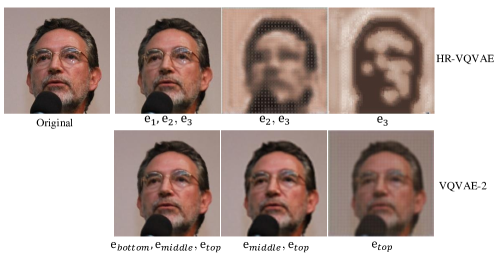
Figure 8: Reconstruction comparison of HR-VQVAE and VQVAE-2.

Table 1 reports the mean squared error (MSE) and fréchet inception distance (FID) [Lucic et al.(2018)Lucic, Kurach, Michalski, Gelly, and Bousquet] results for HR-VQVAE, VQVAE, VQVAE-2 for image reconstructions. The reported scores confirm all the results presented so far. Our proposed HR-VQVAE is able to outperform the baseline models for image reconstructions on all datasets in terms of both MSE and FID score, which is further evidence of the efficiency of our model.

Model	FID $\downarrow$ / MSE $\downarrow$
	FFHQ	ImageNet	CIFAR10	MNIST
VQVAE [Rolfe(2016)]	2.86/0.00298	3.66/0.00055	21.65/0.00092	7.9/0.00041
VQVAE-2 [Razavi et al.(2019)Razavi, van den Oord, and Vinyals]	1.92/0.00195	2.94/0.00039	18.03/0.00068	6.7/0.00025
HR-VQVAE	1.26/0.00163	2.28/0.00027	18.11/0.00041	6.1/0.00011

Table 1: FID/MSE reconstruction results using HR-VQVAE, VQVAE-2 and VQVAE.

As mentioned in the introduction, the hierarchical structure of the codebooks in HR-VQVAE provides fast access to codebook indexes across layers which significantly reduces the search time during decoding. Table 2 reports a comparison of execution time for the high-quality reconstructions of 10000 samples for HR-VQVAE as well as VQVAE and VQVAE-2. The input images are compressed to quantized latent codes of size 32$\times$32 for FFHQ and Imagenet and 16$\times$16 for CIFAR10 and MNIST in HR-VQVAE and VQVAE. For the VQVAE-2 model, the images are compressed into latent codes of size {32$\times$32, 16$\times$16, 8$\times$8} for the bottom, middle, and top layers, respectively for FFHQ and Imagenet and {16$\times$16, 8$\times$8, 4$\times$4}, respectively for CIFAR10 and MNIST. Table 2 reports that HR-VQVAE reaches an over ten-fold increase in reconstruction speed compared to VQVAE-2, and a large improvement with respect to VQVAE. Although HR-VQVAE has codebook sizes of $\{m,m^{2},\dots,m^{n}\}$ in the different layers, it only needs to search through $n\times m$ such vectors due to its hierarchical structure.

Model	Seconds
	FFHQ	Imagenet	CIFAR10	MNIST
VQVAE [Rolfe(2016)]	5.0977652	4.6152677	2.7087896	0.062474
VQVAE-2 [Razavi et al.(2019)Razavi, van den Oord, and Vinyals]	9.3443758	8.8135872	4.4492340	0.090778
HR-VQVAE	0.8398101	0.6714823	0.4667842	0.010830

Table 2: Time for reconstructing 10000 samples using HR-VQVAE, VQVAE-2 and VQVAE.

Fig. 9 presents random samples generated by HR-VQVAE and VQVAE-2. It can be seen that the proposed HR-VQVAE can generate more realistic samples showing the superiority of our model.

HR-VQVAE

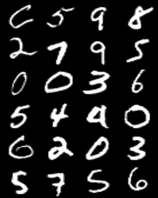
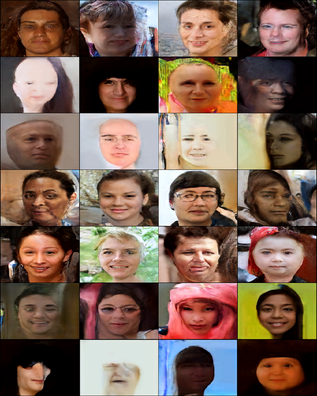
(a) FFHQ

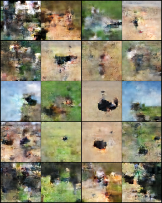
(b) Imagenet

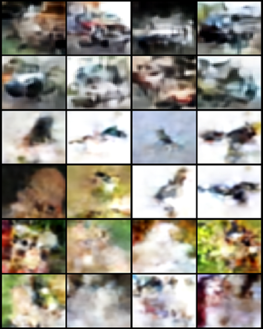
(c) CIFAR10

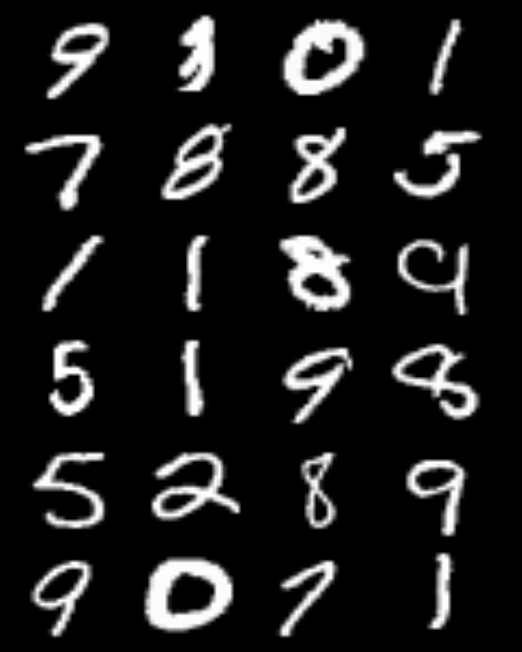
(d) MNIST

Figure 9: Random samples generated by HR-VQVAE and VQVAE-2.

VQVAE-2

Table 3 reports the FID results for generated samples with different models. HR-VQVAE reaches lower FID than the baseline models (VQVAE and VQVAE-2). Furthermore, on FFHQ HR-VQVAE (with PixelCNN for sampling), shows a better performance (17.45) than VDVAE [Child(2020)] and VQGAN [Esser et al.(2021)Esser, Rombach, and Ommer] (with PixelCNN for sampling) which reported FIDs 28.50 and 21.93, respectively, but fails against VQGAN (with Transformer [Katharopoulos et al.(2020)Katharopoulos, Vyas, Pappas, and Fleuret] for sampling) with FID 11.44 which uses a pre-trained autoregressive Transformer to predict rasterized image tokens on the FFHQ dataset. It is worth noting that when VQGAN uses PixelCNN to generate samples, its efficiency is considerably reduced, raising directions for future work.

Model	Generation evaluation (FID $\downarrow$)
	FFHQ	ImageNet	CIFAR10	MNIST
VQVAE [Rolfe(2016)]	24.93	44.76	78.90	16.69
VQVAE-2 [Razavi et al.(2019)Razavi, van den Oord, and Vinyals]	19.66	39.51	74.43	11.81
HR-VQVAE	17.45	35.29	71.38	11.75

Table 3: Generation results using HR-VQVAE, VQVAE-2 and VQVAE.

5 Conclusion

In this paper, we proposed a novel multi-layer variational autoencoder method for image modeling that we call HR-VQVAE. The model learns discrete representations in an iterative and hierarchical fashion. The loss function that we introduce to train the model is designed to encourage different layers to encode different aspects of an image. Through experimental evidence, we show how this model can reconstruct images with a higher level of details than state-of-the-art models with similar complexity. We also show that we can increase the size of the codebooks without incurring the codebook collapse problem that is observed in methods such as VQVAE and VQVAE-2. We visualize the internal representations in the model in an attempt to explain its superior performance. Finally, we show that the hierarchical nature of the codebook design allows to dramatically reduce computation time in decoding.

We believe this model has potential interest for the community both for image reconstruction and generation, particularly in high-load tasks. This is because i) it dramatically compresses the input samples, ii) each layer captures different levels of abstractions, which allows modeling different aspects of the images in parallel, and iii) the search process is sped up by the hierarchical structure of the codebooks.

A Appendix

A.1 Architecture Details and Hyperparameters

	FFHQ ($1024\times 1024$)	Imagenet ($256\times 256$)
Layers	3	2
Latent layers	$\{128\times 128,64\times 64,32\times 32$}	{$64\times 64,32\times 32$}
$\beta_{i}$	0.25	0.25
Hidden units	128	128
Residual units	64	64
Codebook size	64	64
Codebook dimension	64	64
Num. of codewords in layers	{512,512,512}	{512,512,512}
Num. codewords needed for each pixel	$3\times 512$	$3\times 512$
Encoder Conv filter size	3	3
Optimizer	Adam	Adam
Training steps	304741	2207444
Polyak EMA decay	0.9999	0.9999
Learning rate	$2\times{10}^{-4}$	$2\times{10}^{-4}$

Table 4: Hyper parameters of original VQVAE encoder and decoder used for experiments in the original paper.

	FFHQ	Imagenet	CIFAR10	MNIST
Num. of training samples	60,000	1,281,167	50,000	60,000
Num. of test samples	10,000	100,000	10,000	10,000
Input size	$256\times 256\times 3$	$128\times 128\times 3$	$32\times 32\times 3$	$28\times 28\times 1$
Batch size	32	64	128	128
Number of epochs	400	400	999	999
Training steps	875,000	8,007,293	390,234	468,281

Table 5: Input data details for HR-VQVAE and VQVAE2 encoder decoder.

	FFHQ	Imagenet	CIFAR10	MNIST
Layers	3	3	3	3
Latent layers	$32\times 32$	$32\times 32$	$16\times 16$	$16\times 16$
$\beta_{i}$	0.25	0.25	0.25	0.25
Hidden units	128	128	64	64
Residual units	64	64	64	64
Codebook size	8	8	8	4
Codebook dimension	32	32	16	8
Num. of codewords in layers	{8,64,512}	{8,64,512}	{8,64,512}	{4,16,64}
Num. codewords needed for each pixel	$3\times 8$	$3\times 8$	$3\times 8$	$3\times 4$
Encoder Conv filter size	3	3	3	3
Optimizer	Adam	Adam	Adam	Adam
Polyak EMA decay	0.9	0.9	0.9	0.9
Learning rate	$3\times{10}^{-3}$	$3\times{10}^{-3}$	$3\times{10}^{-3}$	$3\times{10}^{-3}$

Table 6: Hyper parameters of 3 layers HR-VQVAE encoder and decoder used for experiments.

	FFHQ	Imagenet	CIFAR10	MNIST
Layers	(Bottom, Mid., Top)	(Bottom, Mid., Top)	(Bottom, Mid., Top)	(Bottom, Mid., Top)
Latent layers	$\{32\times 32,16\times 16,8\times 8\}$	$\{32\times 32,16\times 16,8\times 8\}$	$\{16\times 16,8\times 8,4\times 4\}$	$\{16\times 16,8\times 8,4\times 4\}$
$\beta_{i}$	0.25	0.25	0.25	0.25
Hidden units	128	128	64	64
Residual units	64	64	64	64
Codebook size	512	512	512	64
Codebook dimension	32	32	16	8
Num. of codewords in layers	{512,512,512}	{512,512,512}	{512,512,512}	{64,64,64}
Num. codewords needed for each pixel	$3\times 512$	$3\times 512$	$3\times 512$	$3\times 64$
Encoder Conv filter size	3	3	3	3
Optimizer	Adam	Adam	Adam	Adam
Polyak EMA decay	0.9	0.9	0.9	0.9
Learning rate	$3\times{10}^{-3}$	$3\times{10}^{-3}$	$3\times{10}^{-3}$	$3\times{10}^{-3}$

Table 7: Hyper parameters of 3 layers VQVAE2 encoder and decoder used for experiments.

	FFHQ	Imagenet	CIFAR10	MNIST
Layers	3	3	3	3
Latent layers	$32\times 32$	$32\times 32$	$16\times 16$	$16\times 16$
Batch size	32	128	512	512
Hidden units	128	128	64	64
Residual units	64	64	64	64
Attention layers	4	4	4	4
Attention head	8	8	8	8
Conv. Filter size	5	5	5	5
Dropout	0.15	0.15	0.1	0.1
Output stack layers	0	0	0	0
Polyak EMA decay	0.99	0.99	0.99	0.99

Table 8: Hyper parameters of 3 layers HR-VQVAE autoregressive prior networks used for experiments.

	FFHQ	Imagenet	CIFAR10	MNIST
Layers	(Bottom, Mid., Top)	(Bottom, Mid., Top)	(Bottom, Mid., Top)	(Bottom, Mid., Top)
Latent layers	$\{32\times 32,16\times 16,8\times 8\}$	$\{32\times 32,16\times 16,8\times 8\}$	$\{16\times 16,8\times 8,4\times 4\}$	$\{16\times 16,8\times 8,4\times 4\}$
Batch size	{32, 64, 128}	{64, 128, 256}	512	512
Hidden units	128	128	64	64
Residual units	64	128	64	64
Attention layers	{0, 1, 4}	{0, 1, 4}	{0, 1, 4}	{0, 1, 4}
Attention head	{-,-,8}	{-,-,8}	{-,-,8}	{-,-,8}
Conv. Filter size	{5,5,5}	{5,5,5}	{5,5,5}	{5,5,5}
Dropout	{0.25, 0.3, 0.5}	{0.25, 0.3, 0.5}	{0.25, 0.3, 0.5}	{0.25, 0.3, 0.5}
Output stack layers	0	0	0	0
Polyak EMA decay	0.99	0.99	0.99	0.99

Table 9: Hyper parameters of 3 layers VQVAE2 autoregressive prior networks used for experiments.

Table 4 reports the configuration of VQVAE-2 from the original publication. These models were trained using Google Cloud TPUv3 on FFHQ $1024\times 1024$ and Imagenet $256\times 256$. The original paper reported that such a huge number of parameters were trained using 8 TPU cores and 128 GPUs. In order to perform our comparisons with VQVAE and VQVAE-2, we had to retrain the models. Working in an academic institution, we do not have access to these extensive computational resources. Consequently, the proposed models are much simpler in terms of number of parameters. To make a fair comparison, we retrained VQVAE and VQVAE-2 using a configuration that is more similar to ours.

Table 5 reports information on the input data formats we used in the different data sets. Table 6 reports the hyperparameters for the proposed method (HR-VQVAE) whereas Table 7 reports the hyperparameters that we have used for VQVAE-2. Similarly, Table 8 and Table 9 report the configuration of the autoregressive prior networks used for image generation in HR-VQVAE and VQVAE-2, respectively.

A.2 HR-VQVAE: hierarchy and codebook access

Figure 10 illustrates the idea behind the hierarchical codebooks in the proposed method.

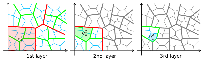
Figure 10: Illustration of the hierarchical codebooks in HR-VQVAE and the speed up in codebook access.

In the example the model has three layers and codebooks of size 4. The plots show layer 1 (left), layer 2 (middle) and layer 3 (right). Also, different color codes are used for codebooks in the layers (red, green and blue, respectively). When a codeword is selected in a certain layer, this limits the codebooks available in the following layers. This is illustrated by graying out the options that are no longer available. In the example, at each layer, the model only has 4 choices, even though the resolution of the last layer has a total of $4^{3}=64$ codewords. This speeds up inference significantly. Finally, note that each layer only models the residual between the original representation and the representation obtained by combining the codewords at previous layers. This gives the name hierarchical residual learning VQVAE to our model.

B Additional samples

This section reports additional samples generated by the various models we have tested. Refer to the figure caption for more information.

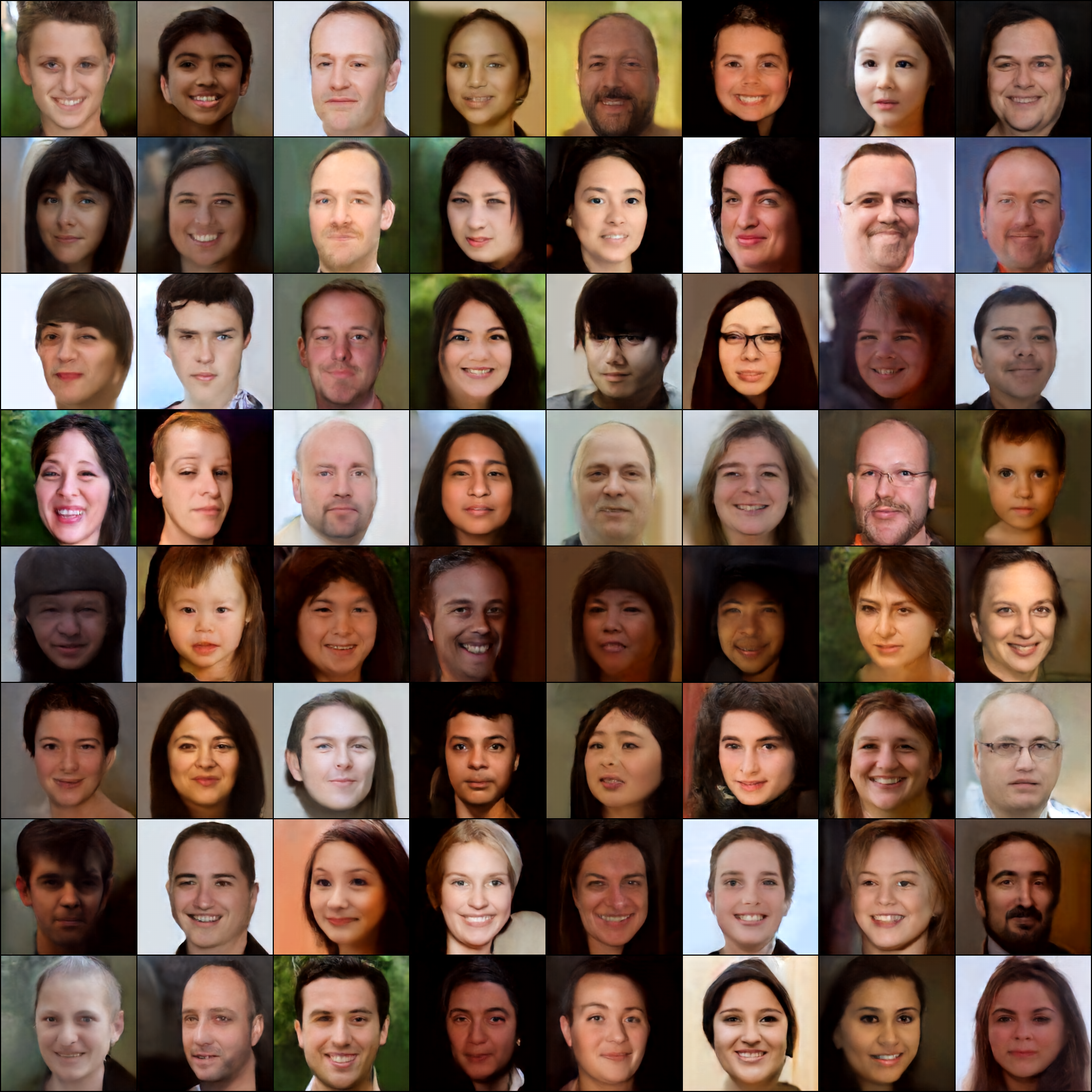
Figure 11: Random samples generated by HR-VQVAE on FFHQ $256\times 256$ dataset.

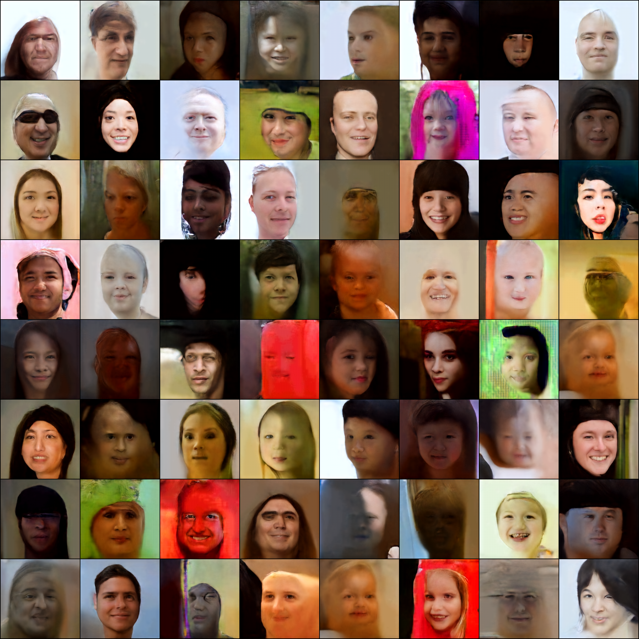
Figure 12: Random samples generated by VQVAE2 on FFHQ $256\times 256$ dataset.

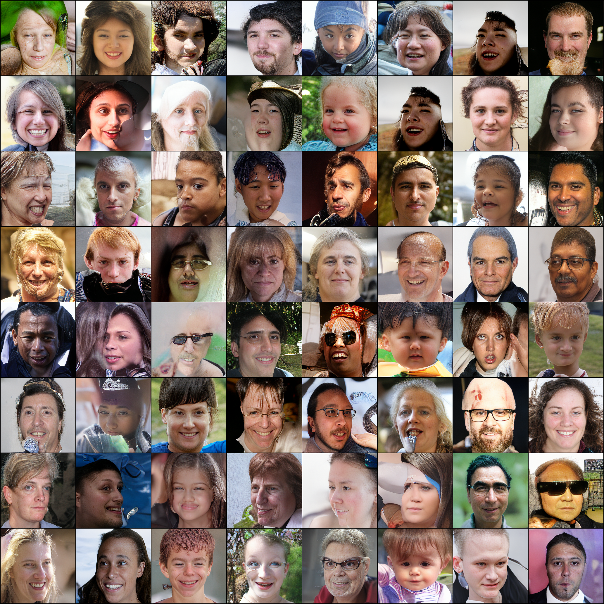
Figure 13: Random samples generated by VQGAN on FFHQ $256\times 256$ dataset.

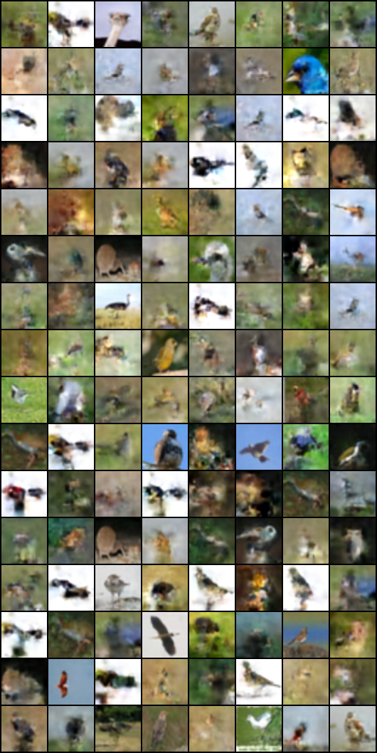
Figure 14: Class conditional random samples generated by HR-VQVAE on CIFAR10-Bird dataset.

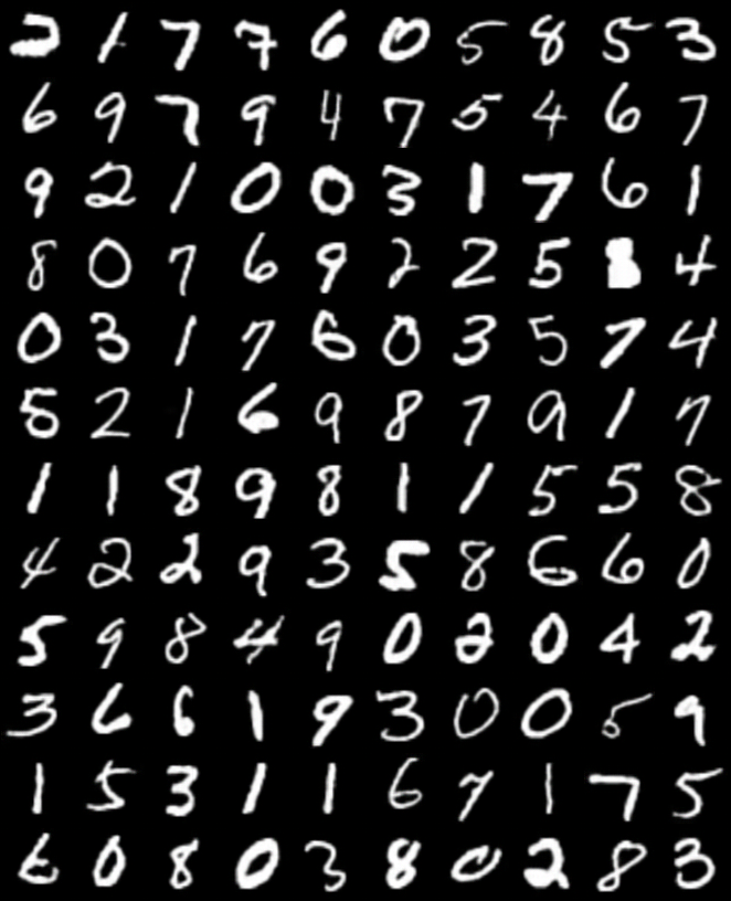
Figure 15: Random samples generated by HR-VQVAE on MNIST dataset.

References

- [Albawi et al.(2017)Albawi, Mohammed, and Al-Zawi] Saad Albawi, Tareq Abed Mohammed, and Saad Al-Zawi. Understanding of a convolutional neural network. In 2017 International Conference on Engineering and Technology (ICET), pages 1–6. Ieee, 2017.
- [Cartuyvels et al.(2021)Cartuyvels, Spinks, and Moens] Ruben Cartuyvels, Graham Spinks, and Marie-Francine Moens. Discrete and continuous representations and processing in deep learning: Looking forward. AI Open, 2:143–159, 2021.
- [Child(2020)] Rewon Child. Very deep vaes generalize autoregressive models and can outperform them on images. arXiv preprint arXiv:2011.10650, 2020.
- [Chorowski et al.(2019)Chorowski, Chen, Marxer, Dolfing, Łańcucki, Sanchez, Alumäe, and Laurent] Jan Chorowski, Nanxin Chen, Ricard Marxer, Hans Dolfing, Adrian Łańcucki, Guillaume Sanchez, Tanel Alumäe, and Antoine Laurent. Unsupervised neural segmentation and clustering for unit discovery in sequential data. In NeurIPS 2019 workshop-Perception as generative reasoning-Structure, Causality, Probability, 2019.
- [Coppock(2020)] Harry Coppock. Vector quantised-variational autoencoders(vq-vaes) for representation learning. 2020.
- [Deng et al.(2009)Deng, Dong, Socher, Li, Li, and Fei-Fei] Jia Deng, Wei Dong, Richard Socher, Li-Jia Li, Kai Li, and Li Fei-Fei. Imagenet: A large-scale hierarchical image database. In 2009 IEEE conference on computer vision and pattern recognition, pages 248–255. Ieee, 2009.
- [Dieleman et al.(2018)Dieleman, van den Oord, and Simonyan] Sander Dieleman, Aaron van den Oord, and Karen Simonyan. The challenge of realistic music generation: modelling raw audio at scale. Advances in Neural Information Processing Systems, 31, 2018.
- [Esser et al.(2021)Esser, Rombach, and Ommer] Patrick Esser, Robin Rombach, and Bjorn Ommer. Taming transformers for high-resolution image synthesis. In Proceedings of the IEEE/CVF conference on computer vision and pattern recognition, pages 12873–12883, 2021.
- [Karras et al.(2019)Karras, Laine, and Aila] Tero Karras, Samuli Laine, and Timo Aila. A style-based generator architecture for generative adversarial networks. In Proceedings of the IEEE/CVF Conference on Computer Vision and Pattern Recognition, pages 4401–4410, 2019.
- [Katharopoulos et al.(2020)Katharopoulos, Vyas, Pappas, and Fleuret] Angelos Katharopoulos, Apoorv Vyas, Nikolaos Pappas, and François Fleuret. Transformers are rnns: Fast autoregressive transformers with linear attention. In International Conference on Machine Learning, pages 5156–5165. PMLR, 2020.
- [Krizhevsky et al.(2009)Krizhevsky, Hinton, et al.] Alex Krizhevsky, Geoffrey Hinton, et al. Learning multiple layers of features from tiny images. 2009.
- [Łańcucki et al.(2020)Łańcucki, Chorowski, Sanchez, Marxer, Chen, Dolfing, Khurana, Alumäe, and Laurent] Adrian Łańcucki, Jan Chorowski, Guillaume Sanchez, Ricard Marxer, Nanxin Chen, Hans JGA Dolfing, Sameer Khurana, Tanel Alumäe, and Antoine Laurent. Robust training of vector quantized bottleneck models. In 2020 International Joint Conference on Neural Networks (IJCNN), pages 1–7. IEEE, 2020.
- [LeCun et al.(1998)LeCun, Bottou, Bengio, and Haffner] Yann LeCun, Léon Bottou, Yoshua Bengio, and Patrick Haffner. Gradient-based learning applied to document recognition. Proceedings of the IEEE, 86(11):2278–2324, 1998.
- [Ledig et al.(2017)Ledig, Theis, Huszár, Caballero, Cunningham, Acosta, Aitken, Tejani, Totz, Wang, et al.] Christian Ledig, Lucas Theis, Ferenc Huszár, Jose Caballero, Andrew Cunningham, Alejandro Acosta, Andrew Aitken, Alykhan Tejani, Johannes Totz, Zehan Wang, et al. Photo-realistic single image super-resolution using a generative adversarial network. In Proceedings of the IEEE conference on computer vision and pattern recognition, pages 4681–4690, 2017.
- [Liang et al.(2017)Liang, Lee, Dai, and Xing] Xiaodan Liang, Lisa Lee, Wei Dai, and Eric P Xing. Dual motion gan for future-flow embedded video prediction. In proceedings of the IEEE international conference on computer vision, pages 1744–1752, 2017.
- [Lucic et al.(2018)Lucic, Kurach, Michalski, Gelly, and Bousquet] Mario Lucic, Karol Kurach, Marcin Michalski, Sylvain Gelly, and Olivier Bousquet. Are gans created equal? a large-scale study. Advances in neural information processing systems, 31, 2018.
- [Mordatch and Abbeel(2018)] Igor Mordatch and Pieter Abbeel. Emergence of grounded compositional language in multi-agent populations. In Thirty-second AAAI conference on artificial intelligence, 2018.
- [Razavi et al.(2019)Razavi, van den Oord, and Vinyals] Ali Razavi, Aaron van den Oord, and Oriol Vinyals. Generating diverse high-fidelity images with vq-vae-2. In Advances in neural information processing systems, pages 14866–14876, 2019.
- [Rolfe(2016)] Jason Tyler Rolfe. Discrete variational autoencoders. arXiv preprint arXiv:1609.02200, 2016.
- [Takahashi et al.(2021)Takahashi, Singh, and Mitsufuji] Naoya Takahashi, Mayank Kumar Singh, and Yuki Mitsufuji. Hierarchical disentangled representation learning for singing voice conversion. arXiv preprint arXiv:2101.06842, 2021.
- [Theis et al.(2016)Theis, van den Oord, and Bethge] L Theis, A van den Oord, and M Bethge. A note on the evaluation of generative models. In International Conference on Learning Representations (ICLR 2016), pages 1–10, 2016.
- [Van den Oord et al.(2016)Van den Oord, Kalchbrenner, Espeholt, Vinyals, Graves, et al.] Aaron Van den Oord, Nal Kalchbrenner, Lasse Espeholt, Oriol Vinyals, Alex Graves, et al. Conditional image generation with pixelcnn decoders. Advances in neural information processing systems, 29, 2016.
- [van den Oord et al.(2017)van den Oord, Vinyals, et al.] Aaron van den Oord, Oriol Vinyals, et al. Neural discrete representation learning. In Advances in Neural Information Processing Systems, pages 6306–6315, 2017.
- [Williams et al.(2020)Williams, Ringer, Ash, Hughes, MacLeod, and Dougherty] Will Williams, Sam Ringer, Tom Ash, John Hughes, David MacLeod, and Jamie Dougherty. Hierarchical quantized autoencoders. arXiv preprint arXiv:2002.08111, 2020.
- [Zhang and Wu(2005)] Lei Zhang and Xiaolin Wu. Color demosaicking via directional linear minimum mean square-error estimation. IEEE Transactions on Image Processing, 14(12):2167–2178, 2005.
- [Zhao et al.(2017)Zhao, Song, and Ermon] Shengjia Zhao, Jiaming Song, and Stefano Ermon. Towards deeper understanding of variational autoencoding models. arXiv preprint arXiv:1702.08658, 2017.
- [Zhao et al.(2020)Zhao, Yu, Mahapatra, Su, and Chen] Yang Zhao, Ping Yu, Suchismit Mahapatra, Qinliang Su, and Changyou Chen. Improve variational autoencoder for text generation with discrete latent bottleneck. arXiv preprint arXiv:2004.10603, 2020.