Gravity in binary systems at the fifth and sixth post-Newtonian order

Abstract

Binary sources of gravitational waves in the early inspiral phase are accurately described by a post-Newtonian expansion in small velocity and weak interaction. We compute the conservative dynamics to fifth and partial sixth order using a non-relativistic effective field theory. We give predictions for central observables and determine the required coefficients for the construction of an Effective One-Body Hamiltonian, extending the applicability of our results to the late inspiral and merger phases.

1 Introduction

Accurate wave form templates are indispensible to determine the properties of binary black hole or neutron star systems at gravitational wave observatories. The construction of such templates requires a detailed understanding of all phases of binary mergers.

Here, we mainly focus on binary systems of point-like objects without spin in the early inspiral phase, characterised by a large separation and small velocities. As a first approximation, the system can be considered Newtonian with energy

$$E_{N}=\mu\left(\frac{\mathrm{v}^{2}}{2}-\frac{GM}{r}\right)$$ (1)

in the centre-of-mass frame. $M=m_{1}+m_{2}$ is the sum of the constituent masses $m_{1},m_{2}$, $\mu=\frac{m_{1}m_{2}}{M}$ the reduced mass, $\mathrm{v}$ the relative velocity, $G$ Newton’s constant, and $r$ the orbital separation. To obtain relativistic corrections, we perform a post-Newtonian (PN) expansion in $\mathrm{v}\sim\sqrt{\frac{GM}{r}}\ll 1$, where the correlation between velocity and interaction strength follows directly from the virial theorem for equation (1).

Using a non-relativistic effective theory, the dynamics of compact binary systems in the post-Newtonian expansion can be computed in terms of Feynman diagrams. We briefly outline this approach and present results for the binding energy and the periastron advance at the fifth post-Newtonian order. We also derive the local-in-time contributions to the scattering angle for unbound systems and determine the coefficients of an Effective One-Body (EOB) Hamiltonian, which allows to predict the dynamics far beyond the validity range of the post-Newtonian expansion.

2 Effective Field Theory Framework

2.1 General Relativity

Our starting point is the $d$-dimensional general relativity action in harmonic gauge, coupled to point-like matter:

$$S_{\text{GR}}[g^{\mu\nu}]=\frac{1}{16G\pi}\int d^{d}x\sqrt{-g}\left(R-\frac{1}{2}\Gamma_{\mu}\Gamma^{\mu}\right)+\sum_{a=1}^{2}m_{a}\int d\tau_{a}.$$ (2)

We use natural units, $c=\hbar=1$, keeping the dependence on Newton’s constant $G$ explicit. The only dynamic field is the metric $g^{\mu\nu}$ with determinant $g$. In the limit of flat four-dimensional spacetime, $g^{\mu\nu}\to\eta^{\mu\nu},d\to 4$, we choose the signature $\eta^{\mu\nu}=\operatorname{diag}(-1,1,1,1)$. $R$ is the Ricci scalar and $\Gamma^{\mu}=g^{\alpha\beta}\Gamma^{\mu}_{\alpha\beta}$ a contracted Christoffel symbol. $\tau_{a}$ is the proper time of the compact object $a$.

Before constructing an effective field theory, we perform a post-Newtonian expansion of the general relativity action. We employ the convenient parametrisation [1]

$$g^{\mu\nu}=e^{2{\color[rgb]{0,0,1}\tilde{\phi}}}\begin{pmatrix}-1&{\color[rgb]{1,0,0}\tilde{A}_{j}}\\ {\color[rgb]{1,0,0}\tilde{A}_{i}}&e^{-c_{d}{\color[rgb]{0,0,1}\tilde{\phi}}}(\delta_{ij}+{\color[rgb]{0,0.5,0}\tilde{\sigma}_{ij}})-{\color[rgb]{1,0,0}\tilde{A}_{i}\tilde{A}_{j}}\end{pmatrix}\,,\qquad c_{d}=2\frac{d-2}{d-3}$$ (3)

with ${\color[rgb]{0,0,1}\tilde{\phi}}\sim{\color[rgb]{1,0,0}\tilde{A}}\sim{\color[rgb]{0,0.5,0}\tilde{\sigma}}\sim\sqrt{\frac{GM}{r}}$.

Introducing the Planck mass $m_{\text{Pl}}=\frac{1}{\sqrt{32\pi G}}$ and rescaling $({\color[rgb]{0,0,1}\tilde{\phi}},{\color[rgb]{1,0,0}\tilde{A}},{\color[rgb]{0,0.5,0}\tilde{\sigma}})=\frac{1}{m_{\text{Pl}}}({\color[rgb]{0,0,1}\phi},{\color[rgb]{1,0,0}A},{\color[rgb]{0,0.5,0}\sigma})$ we arrive at

$$\begin{split}&S_{\text{GR}}[{\color[rgb]{0,0,1}\phi},{\color[rgb]{1,0,0}A},{\color[rgb]{0,0.5,0}\sigma}]=\int dt\ \overbrace{\sum_{a=1}^{2}\left(m_{a}+\frac{1}{2}m_{a}\mathrm{v}_{a}^{2}+\dots\right)}^{M+T}\\ &\qquad+\int dt\ \sum_{a=1}^{2}\frac{m_{a}}{m_{\text{Pl}}}\left(-{\color[rgb]{0,0,1}\phi}(t,\vec{x}_{a})+(\mathrm{v}_{a})_{i}{\color[rgb]{1,0,0}A_{i}}(t,\vec{x}_{a})+(\mathrm{v}_{a})_{i}(\mathrm{v}_{a})_{j}{\color[rgb]{0,0.5,0}\sigma_{ij}}(t,\vec{x}_{a})-\frac{1}{2m_{\text{Pl}}}{\color[rgb]{0,0,1}\phi}(t,\vec{x}_{a})^{2}+\dots\right)\\ &\qquad+\int d^{d}x\ \left[-c_{d}\bigl{(}\partial_{\mu}{\color[rgb]{0,0,1}\phi}(x)\bigr{)}^{2}+\bigl{(}\partial_{\mu}{\color[rgb]{1,0,0}A_{i}}(x)\bigr{)}^{2}+\frac{1}{4}\bigl{(}\partial_{\mu}{\color[rgb]{0,0.5,0}\sigma_{ii}}(x)\bigr{)}^{2}-\frac{1}{2}\bigl{(}\partial_{\mu}{\color[rgb]{0,0.5,0}\sigma_{ij}}(x)\bigr{)}^{2}+\dots\right],\end{split}$$ (4)

where the ellipses indicate higher-order terms omitted for brevity here. The first line of equation (4) describes the matter dynamics, the second line the interaction between matter and gravitational field, and the third line the bulk field dynamics.

To achieve a consistent expansion, we have to decompose each field into hard, soft, potential, and radiation (or ultrasoft) modes [2]. However, hard and soft modes only contribute through quantum corrections and can be safely neglected. The decomposition into modes therefore reads

$$({\color[rgb]{0,0,1}\phi},{\color[rgb]{1,0,0}A},{\color[rgb]{0,0.5,0}\sigma})={} ({\color[rgb]{0,0,1}\phi_{\text{pot}}},{\color[rgb]{1,0,0}A_{\text{pot}}},{\color[rgb]{0,0.5,0}\sigma_{\text{pot}}})+({\color[rgb]{0,0,1}\phi_{\text{rad}}},{\color[rgb]{1,0,0}A_{\text{rad}}},{\color[rgb]{0,0.5,0}\sigma_{\text{rad}}}),$$ (5)

$$\partial_{i}({\color[rgb]{0,0,1}\phi_{\text{pot}}},{\color[rgb]{1,0,0}A_{\text{pot}}},{\color[rgb]{0,0.5,0}\sigma_{\text{pot}}})\sim{} \frac{1}{r}({\color[rgb]{0,0,1}\phi_{\text{pot}}},{\color[rgb]{1,0,0}A_{\text{pot}}},{\color[rgb]{0,0.5,0}\sigma_{\text{pot}}}),$$ (6)

$$\partial_{0}({\color[rgb]{0,0,1}\phi_{\text{pot}}},{\color[rgb]{1,0,0}A_{\text{pot}}},{\color[rgb]{0,0.5,0}\sigma_{\text{pot}}})\sim{} \frac{\mathrm{v}}{r}({\color[rgb]{0,0,1}\phi_{\text{pot}}},{\color[rgb]{1,0,0}A_{\text{pot}}},{\color[rgb]{0,0.5,0}\sigma_{\text{pot}}}),$$ (7)

$$\partial_{\mu}({\color[rgb]{0,0,1}\phi_{\text{rad}}},{\color[rgb]{1,0,0}A_{\text{rad}}},{\color[rgb]{0,0.5,0}\sigma_{\text{rad}}})\sim{} \frac{\mathrm{v}}{r}({\color[rgb]{0,0,1}\phi_{\text{rad}}},{\color[rgb]{1,0,0}A_{\text{rad}}},{\color[rgb]{0,0.5,0}\sigma_{\text{rad}}}).$$ (8)

2.2 Non-Relativistic General Relativity

We now seek to construct a physically equivalent effective field theory without potential modes. This effective theory, termed Non-Relativistic General Relativity (NRGR) [3], has an action of the form

$$S_{\text{NRGR}}[{\color[rgb]{0,0,1}\phi_{\text{rad}}},{\color[rgb]{1,0,0}A_{\text{rad}}},{\color[rgb]{0,0.5,0}\sigma_{\text{rad}}}]=S_{\text{matter}}+S_{\text{mult}}+S_{\text{bulk, rad}},$$ (9)

where

$$S_{\text{matter}}=\int dt\ (M+T-V_{\text{NZ}})$$ (10)

describes the matter and its interactions via the classical near-zone potential $V_{\text{NZ}}$, $S_{\text{mult}}$ the multipole-expanded interactions between matter and radiation modes, and $S_{\text{bulk, rad}}$ the bulk dynamics of the radiation modes. Indeed, $S_{\text{bulk, rad}}$ is identical to the general relativity bulk action after setting the potential modes to zero. Demanding equivalence to general relativity within the post-Newtonian expansion leads to the matching condition

$$V_{\text{NZ}}=i\frac{d}{dt}\log\left[\frac{1}{Z}\int\mathcal{D}{\color[rgb]{0,0,1}\phi_{\text{pot}}}\mathcal{D}{\color[rgb]{1,0,0}A_{\text{pot}}}\mathcal{D}{\color[rgb]{0,0.5,0}\sigma_{\text{pot}}}\ e^{i\left[S_{\text{GR}}-\int dt(M+T)\right]_{{\color[rgb]{0,0,1}\phi_{\text{rad}}}={\color[rgb]{1,0,0}A_{\text{rad}}}={\color[rgb]{0,0.5,0}\sigma_{\text{rad}}}=0}}\right].$$ (11)

After inserting the action from equation (4) we obtain the following diagrammatic expansion

$$V_{\text{NZ}}=i\frac{d}{dt}\Biggl{[}\ \underbrace{\vbox{\hbox{\includegraphics{pot_tree_p_label_source}}}}_{0\text{PN}}\ +\ \underbrace{\vbox{\hbox{\includegraphics{pot_tree_A_label_source}}}\ +\ \frac{1}{2}\times\vbox{\hbox{\includegraphics{pot_1l_seagull_source}}}\ +\ \frac{1}{2}\times\vbox{\hbox{\includegraphics{pot_1l_seagull_source_rev}}}}_{1\text{PN}}\ +\ (2\text{PN})\ \Biggr{]}\\$$ (12)

Crossed circles indicate classical sources, i.e. interactions with compact object 1 at the top and object 2 at the bottom. Inserting the Feynman rules leads to Fourier transforms of massless propagator-type Feynman diagrams in $d-1$ space dimensions. Generally, Diagrams with $L+2$ sources in equation (12) first contribute at $L$PN order and correspond to $L$-loop propagator diagrams.

We have computed the full 5PN contributions with up to five loops [6, 7, 8] and 6PN contributions with up to three loops [9, 10] to $V_{\text{NZ}}$. Diagrams are generated with QGRAF [11], manipulated with the help of FORM [12, 13], and reduced to master integrals using a custom implementation [14] of Laporta’s algorithm [15] for integration-by-parts reduction [16]. Only one of the master integrals cannot be calculated with elementary methods; it was first computed in [17]. The result for $V_{\text{NZ}}$ initially contains higher-order time derivatives, which we systematically eliminate through integration by parts, multiple-zero insertions, and coordinate shifts. We find full agreement with independent partial PN calculations [4, 5] and a post-Minkowskian expansion to fourth order [18, 19, 20, 21].

2.2.1 Post-Newtonian Mechanics

Finally, we integrate out the remaining radiation modes, projecting onto the conservative contribution to the action. We arrive at a post-Newtonian action of the form

$$S_{\text{PN}}=\int dt\ L[\vec{r},\vec{\mathrm{v}}]=\int dt\ (M+T-V_{\text{NZ}}+L_{\text{FZ}}),$$ (13)

where the far-zone Lagrangian $L_{\text{FZ}}$ is obtained from the NRGR action, equation (9), through the matching condition

$$L_{\text{FZ}}=-i\frac{d}{dt}\log\left[\frac{1}{\tilde{Z}}\int\mathcal{D}{\color[rgb]{0,0,1}\phi_{\text{rad}}}\mathcal{D}{\color[rgb]{1,0,0}A_{\text{rad}}}\mathcal{D}{\color[rgb]{0,0.5,0}\sigma_{\text{rad}}}\ e^{iS_{\text{rad}}}\right]_{\text{cons}},$$ (14)

where $S_{\text{rad}}=S_{\text{mult}}+S_{\text{bulk, rad}}$. The subscript indicates projection onto the conservative contribution. $S_{\text{mult}}$ describes the interactions between matter and radiation modes in NRGR. Since the wave length of the radiation modes is parametrically larger than the orbital separation and the wave length of the potential modes, c.f. equations (6) and (8), this contribution to the action has to be multipole-expanded. In the centre-of-mass frame one obtains in $d$ dimensions [22, 23]

$$\begin{split}S_{\text{mixed}}=\int dt\ &\left[\frac{1}{2}{E}\delta g_{00}(t,\vec{0})-\frac{1}{2}{L^{i|j}}\partial_{j}\delta g_{0i}(t,\vec{0})-\frac{1}{2}{Q^{ij}}R_{0i0j}(t,\vec{0})\right.\\ &\left.-\frac{1}{3}{J^{i|jk}}R_{0jki}(t,\vec{0})-\frac{1}{6}{O^{ijk}}\partial_{k}R_{0i0j}(t,\vec{0})+\dots\right],\end{split}$$

where $R^{\mu}_{\phantom{\mu}\nu\rho\sigma}$ is the Riemann tensor, expanded in powers of $\delta g_{\mu\nu}=g_{\mu\nu}-\eta_{\mu\nu}$. We again use the parametrisation defined in equation (3) for the metric, replacing $({\color[rgb]{0,0,1}\phi},{\color[rgb]{1,0,0}A},{\color[rgb]{0,0.5,0}\sigma})\to({\color[rgb]{0,0,1}\phi_{\text{rad}}},{\color[rgb]{1,0,0}A_{\text{rad}}},{\color[rgb]{0,0.5,0}\sigma_{\text{rad}}})$. We distinguish between mass-type (“electric”) multipole moments $E,P^{i}=0,Q^{ij},O^{ijk}$ which are symmetric under permutation of indices, and current-type (“magnetic”) multipole moments $L^{i|j},J^{i|jk}$ which are antisymmetric under index exchanges crossing the vertical bar. In principle, further evanescent multipole moments arise for $d\neq 4$. However, they do not contribute at 5PN order.

To disentangle conservative and dissipative effects we employ the closed-time-path (or in-in) formalism, replacing

$$S_{\text{rad}}[{\color[rgb]{0,0,1}\phi_{\text{rad}}},{\color[rgb]{1,0,0}A_{\text{rad}}},{\color[rgb]{0,0.5,0}\sigma_{\text{rad}}},\vec{r},\vec{\mathrm{v}}]\to S_{\text{rad}}[{\color[rgb]{0,0,1}\phi_{\text{rad},1}},{\color[rgb]{1,0,0}A_{\text{rad},1}},{\color[rgb]{0,0.5,0}\sigma_{\text{rad},1}},\vec{r}_{1},\vec{\mathrm{v}}_{1}]-S_{\text{rad}}[{\color[rgb]{0,0,1}\phi_{\text{rad},2}},{\color[rgb]{1,0,0}A_{\text{rad},2}},{\color[rgb]{0,0.5,0}\sigma_{\text{rad},2}},\vec{r}_{2},\vec{\mathrm{v}}_{2}]$$ (15)

in the matching equation (14), cf. [24]. Note that the subscripts here indicate the time path and are unrelated to the indices associated with the compact objects.

From equation (14) we obtain

$$L_{\text{FZ}}=-i\frac{d}{dt}\left[\ \vbox{\hbox{\includegraphics{L_FZ_lin}}}\ +\ \vbox{\hbox{\includegraphics{L_FZ_quad}}}\ \right]_{\text{cons}},$$ (16)

where the lines denote retarded or advanced propagators of ${\color[rgb]{0,0,1}\phi_{\text{rad}}},{\color[rgb]{1,0,0}A_{\text{rad}}}$, or ${\color[rgb]{0,0.5,0}\sigma_{\text{rad}}}$ and the crossed circles are interactions with the multipole moments of the binary system. At 4PN order, only the combination of one coupling to the energy $E$ and two couplings to the mass quadrupole $Q_{ij}$ contributes, while at 5PN order all of the multipole moments in equation (2.2.1) appear. This implies that $d$-dimensional expressions including 1PN corrections are required for $E$ and $Q$ [25], whereas the Newtonian level is sufficient for the remaining multipole moments. Retaining only terms that are linear in $\vec{r}_{-}=\frac{1}{\sqrt{2}}(\vec{r}_{1}-\vec{r}_{2})$, the result has the form

$$L_{\text{FZ}}=-i\frac{d}{dt}\bigg{[}S_{\text{hom}}[\vec{r}_{1},\vec{\mathrm{v}}_{1}]-S_{\text{hom}}[\vec{r}_{2},\vec{\mathrm{v}}_{2}]+S_{\text{inhom}}[\vec{r}_{1},\vec{r}_{2},\vec{\mathrm{v}}_{1},\vec{\mathrm{v}}_{2}]\bigg{]}_{\text{cons}}.$$ (17)

We identify $S_{\text{hom}}$ with the conservative contribution [26]. Note that $L_{\text{FZ}}$ can be subdivided into a part $L_{\text{FZ, loc}}$ describing local-in-time, i.e. instantaneous, interactions and a non-local part $L_{\text{FZ, nl}}$ containing a time integral that cannot be evaluated in closed form without specifying a trajectory.

3 Observables

After a Legendre transform, we obtain a Hamiltonian, from which we predict physical observables. We briefly review our main results; for a detailed account see [24].

First, we consider an elliptic orbit in the limit of vanishing eccentricity. The binding energy is given by

$$E^{\text{circ}}=E^{\text{circ}}_{\text{loc}}+E^{\text{circ}}_{\text{nl}},$$ (18)

where $E^{\text{circ}}_{\text{loc}}$ and $E^{\text{circ}}_{\text{nl}}$ denote the contributions originating from local and non-local in time Hamiltonian parts, respectively. Expressed in terms of the reduced angular momentum $j=\frac{J}{GM}$ and $\nu=\frac{\mu}{M}$ they read

$$\begin{split}\frac{E_{\text{loc}}^{\text{circ}}(j)}{\mu}={}&-\frac{1}{2j^{2}}+\left(-\frac{\nu}{8}-\frac{9}{8}\right)\frac{1}{j^{4}}+\left(-\frac{\nu^{2}}{16}+\frac{7\nu}{16}-\frac{81}{16}\right)\frac{1}{j^{6}}+\Biggl{[}-\frac{5\nu^{3}}{128}+\frac{5\nu^{2}}{64}+\Biggl{(}\frac{8833}{384}-\frac{41\pi^{2}}{64}\Biggr{)}\nu\\ &-\frac{3861}{128}\Biggr{]}\frac{1}{j^{8}}+\Biggl{[}-\frac{7\nu^{4}}{256}+\frac{3\nu^{3}}{128}+\left(\frac{41\pi^{2}}{128}-\frac{8875}{768}\right)\nu^{2}+\Biggl{(}\frac{989911}{3840}-\frac{6581\pi^{2}}{1024}\Biggr{)}\nu\\ &-\frac{53703}{256}\Biggr{]}\frac{1}{j^{10}}+{\Biggl{[}-\frac{21\nu^{5}}{1024}+\frac{5\nu^{4}}{1024}+\Biggl{(}\frac{41\pi^{2}}{512}-\frac{3769}{3072}\Biggr{)}\nu^{3}}\Biggl{(}-\frac{400383799}{403200}+\frac{132979\pi^{2}}{2048}\Biggr{)}\nu^{2}\\ &+\Biggl{(}\frac{3747183493}{1612800}-\frac{31547\pi^{2}}{1536}\Biggr{)}\nu-\frac{1648269}{1024}\Biggr{]}\frac{1}{j^{12}}+\mathcal{O}\left(\frac{1}{j^{14}}\right),\end{split}$$ (19)

$$\begin{split}\frac{E^{\text{circ}}_{\text{nl}}}{\mu}={}&\nu\Biggl{\{}\Biggl{[}-\frac{64}{5}(\ln(j)-\gamma_{E})+\frac{128}{5}\ln(2)\Biggr{]}\frac{1}{j^{10}}+\Biggl{[}\frac{32}{5}+\frac{28484}{105}\ln(2)+\frac{243}{14}\ln(3)\\ &-\frac{15172}{105}(\ln(j)-\gamma_{E})+\nu\Biggl{(}\frac{32}{5}+\frac{112}{5}(\ln(j)-\gamma_{E})+\frac{912}{35}\ln(2)-\frac{486}{7}\ln(3)\Biggr{)}\Biggr{]}\frac{1}{j^{12}}\Biggr{\}}\\ &+\mathcal{O}\left(\frac{1}{j^{14}}\right)\end{split}$$ (20)

up to 5PN order. Similarly, the 5PN periastron advance in this limit is given by

$$K^{\text{circ}}(j)={} K^{\text{circ}}_{\text{loc}}(j)+K^{\text{circ}}_{\text{nl}}(j),$$ (21)

$$K^{\text{circ}}_{\text{loc}}(j)={} 1+3\frac{1}{j^{2}}+\Biggl{(}\frac{45}{2}-6\nu\Biggr{)}\frac{1}{j^{4}}+\Biggl{[}\frac{405}{2}+\Biggl{(}-202+\frac{123}{32}\pi^{2}\Biggr{)}\nu+3\nu^{2}\Biggr{]}\frac{1}{j^{6}}$$

$$+\Biggl{[}\frac{15795}{8}+\left(\frac{185767}{3072}\pi^{2}-\frac{105991}{36}\right)\nu+\Biggl{(}-\frac{41}{4}\pi^{2}+\frac{2479}{6}\Biggr{)}\nu^{2}\Biggr{]}\frac{1}{j^{8}}$$

$$+{\Biggl{[}\frac{161109}{8}}+\Biggl{(}-\frac{18144676}{525}+\frac{488373}{2048}\pi^{2}\Biggr{)}\nu-\Biggl{(}\frac{15079451}{675}+\frac{1379075}{1024}\pi^{2}\Biggr{)}\nu^{2}$$

$$+\Biggl{(}-\frac{1627}{6}+\frac{205}{32}\pi^{2}\Biggr{)}\nu^{3}\Biggr{]}\frac{1}{j^{10}}+O\left(\frac{1}{j^{12}}\right),$$ (22)

$$K^{\text{circ}}_{\text{nl}}(j)={} -\frac{64}{10}\nu\Biggl{\{}\frac{1}{j^{8}}\Biggl{[}-11-\frac{157}{6}(\ln(j)-\gamma_{E})+\frac{37}{6}\ln(2)+\frac{729}{16}\ln(3)\Biggr{]}$$

$$+{\frac{1}{j^{10}}\Biggl{[}-\frac{59723}{336}-\frac{9421}{28}[\ln(j)-\gamma_{E}]+\frac{7605}{28}\ln(2)+\frac{112995}{224}\ln(3)}$$

$${+\Biggl{(}\frac{2227}{42}+\frac{617}{6}[\ln(j)-\gamma_{E}]-\frac{7105}{6}\ln(2)+\frac{54675}{112}\ln(3)\Biggr{)}\nu\Biggr{]}}+O\left(\frac{1}{j^{12}}\right).$$ (23)

Both observables are shown in figure 1 as functions of $x=(GM\Omega)^{\frac{2}{3}}$, where $\Omega$ is the angular orbital frequency with $GM\Omega=\frac{1}{\mu}\frac{dE^{\text{circ}}}{dj}$, see e.g. [27].

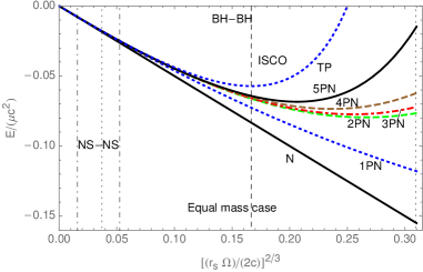
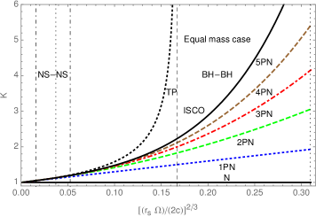
Figure 1: Energy (left) and Periastron advance (right) as functions of $x=(GM\Omega)^{\frac{2}{3}}$ in the quasi-circular case for equal masses. The uppermost dashed line denotes the exact result in the test particle limit, where the innermost stable circular orbit (ISCO) is marked by a dashed vertical line. The solid black lines and curves in between show predictions from successive post-Newtonian orders. The dotted and dash-dotted vertical lines illustrate the frequency ranges for binary black-hole and neutron star systems covered by current experiments. Figure reproduced from [24].

The frequency, or equivalently $x$, for the innermost stable circular orbit (ISCO) is found by minimising the energy, $\frac{dE^{\text{circ}}}{dx}=0$. In the test particle limit $m_{2}\to 0$ one finds

$$\frac{E^{\text{circ}}_{\text{TP}}}{\mu}=\frac{1-2x}{\sqrt{1-3x}}-1,\qquad x^{\text{ISCO}}_{\text{TP}}=\frac{1}{6}.$$ (24)

To obtain an $n$PN-accurate expression for the circular binding energy with arbitrary masses, we define

$$E^{\text{circ}}_{\text{TP}+n\text{PN}\nu}=E^{\text{circ}}_{\text{TP}}-E^{\text{circ}}_{\text{TP},n\text{PN}}+E^{\text{circ}}_{n\text{PN}},$$ (25)

where $E^{\text{circ}}_{\text{TP},n\text{PN}}$ is $E^{\text{circ}}_{\text{TP}}$ expanded to $n$PN order and $E^{\text{circ}}_{n\text{PN}}$ is the $n$PN approximation to the circular binding energy. For the ISCO frequency we then obtain

$$x^{\text{ISCO}}_{\text{TP}+1\text{PN}\nu}\approx{} 0.16625696117738773332,$$ (26)

$$x^{\text{ISCO}}_{\text{TP}+2\text{PN}\nu}\approx{} 0.16918429803993408276,$$ (27)

$$x^{\text{ISCO}}_{\text{TP}+3\text{PN}\nu}\approx{} 0.18096727401354580502,$$ (28)

$$x^{\text{ISCO}}_{\text{TP}+4\text{PN}\nu}\approx{} 0.18807765161857146375,$$ (29)

$$x^{\text{ISCO}}_{\text{TP}+5\text{PN}\nu}\approx{} 0.18788220419180782864.$$ (30)

We compare our results to the local-in-time EOB Hamiltonian [28], viz.

$$H_{\text{EOB}}^{\text{loc}}={} \sqrt{A(1+p^{2}+(AD-1)p_{r}^{2}+Q)},$$ (31)

$$A={} 1+\sum_{k=1}^{6}\frac{a_{k}}{r^{k}},$$ (32)

$$D={} 1+\sum_{k=2}^{5}\frac{d_{k}}{r^{k}},$$ (33)

$$Q={} p_{r}^{4}\left[\frac{q_{42}}{r^{2}}+\frac{q_{43}}{r^{3}}+\frac{q_{44}}{r^{4}}\right]+p_{r}^{6}\left[\frac{q_{62}}{r^{2}}+\frac{q_{63}}{r^{3}}\right]+p_{r}^{8}\frac{q_{82}}{r^{2}}$$ (34)

to 5PN, where $p_{r}$ denotes the radial component of the spatial momentum and $r=\frac{r_{\text{phys}}}{GM}$ is the rescaled orbital separation. Comparing to our results for the circular binding energy and the local periastron advance $K^{\text{loc}}(E,j)$ beyond the circular limit we derive all 5PN EOB parameters:

$$q_{82}={} \frac{6}{7}\nu+\frac{18}{7}\nu^{2}+\frac{24}{7}\nu^{3}-6\nu^{4},$$ (35)

$$q_{63}={} \frac{123}{10}\nu-\frac{69}{5}\nu^{2}+116\nu^{3}-14\nu^{4},$$ (36)

$$q_{44}={} \left(\frac{1580641}{3150}-\frac{93031\pi^{2}}{1536}\right)\nu+\left({-\frac{3670222}{4725}}+\frac{31633\pi^{2}}{512}\right)\nu^{2}+\left(640-\frac{615}{32}\pi^{2}\right)\nu^{3},$$ (37)

$$d_{5}={} \left(\frac{331054}{175}-\frac{63707}{512}\pi^{2}\right)\nu+\left({-\frac{31295104}{4725}}+\frac{306545}{512}\pi^{2}\right)\nu^{2}+\left(\frac{1069}{3}-\frac{205}{16}\pi^{2}\right)\nu^{3},$$ (38)

$$a_{6}={} \left(-\frac{1026301}{1575}+\frac{246367}{3072}\pi^{2}\right)\nu+\left({-\frac{1749043}{1575}}+\frac{25911}{256}\pi^{2}\right)\nu^{2}+4\nu^{3}.$$ (39)

All other coefficients in eqs. (32), (33), (34) are already determined up to 4PN. The predictions for the terms proportional to $\nu^{2}$ in $d_{5}$ and $a_{6}$ have not been obtained in any other approach so far.

Moving beyond a closed orbit, we compute the PN expansion of the scattering angle $\chi$. Explicit formulae are given in [24]. For the most part, we find agreement with other determinations [29, 30, 31], except for a deviation that can be traced back to the rational contribution of order $\nu^{2}$ to $q_{44}$. This numerically small difference, cf. [32], is under investigation. Note that it has not yet been proven that one can perform an analytic continuation of the Hamiltonian dynamics from scattering to the bound state problem from 5PN onward.

References

- [1] B. Kol and M. Smolkin, Classical Effective Field Theory and Caged Black Holes, Phys. Rev. D 77 (2008) 064033 [0712.2822].
- [2] M. Beneke and V. A. Smirnov, Asymptotic expansion of Feynman integrals near threshold, Nucl. Phys. B 522 (1998) 321 [hep-ph/9711391].
- [3] W. D. Goldberger and I. Z. Rothstein, An Effective field theory of gravity for extended objects, Phys. Rev. D 73 (2006) 104029 [hep-th/0409156].
- [4] S. Foffa, P. Mastrolia, R. Sturani, C. Sturm and W. J. Torres Bobadilla, Static two-body potential at fifth post-Newtonian order, Phys. Rev. Lett. 122 (2019) 241605 [1902.10571].
- [5] S. Foffa, R. Sturani and W. J. Torres Bobadilla, Efficient resummation of high post-Newtonian contributions to the binding energy, JHEP 02 (2021) 165 [2010.13730].
- [6] J. Blümlein, A. Maier and P. Marquard, Five-Loop Static Contribution to the Gravitational Interaction Potential of Two Point Masses, Phys. Lett. B 800 (2020) 135100 [1902.11180].
- [7] J. Blümlein, A. Maier, P. Marquard and G. Schäfer, Fourth post-Newtonian Hamiltonian dynamics of two-body systems from an effective field theory approach, Nucl. Phys. B 955 (2020) 115041 [2003.01692].
- [8] J. Blümlein, A. Maier, P. Marquard and G. Schäfer, The fifth-order post-Newtonian Hamiltonian dynamics of two-body systems from an effective field theory approach: potential contributions, Nucl. Phys. B 965 (2021) 115352 [2010.13672].
- [9] J. Blümlein, A. Maier, P. Marquard and G. Schäfer, Testing binary dynamics in gravity at the sixth post-Newtonian level, Phys. Lett. B 807 (2020) 135496 [2003.07145].
- [10] J. Blümlein, A. Maier, P. Marquard and G. Schäfer, The 6th post-Newtonian potential terms at , Phys. Lett. B 816 (2021) 136260 [2101.08630].
- [11] P. Nogueira, Automatic Feynman graph generation, J. Comput. Phys. 105 (1993) 279.
- [12] J. A. M. Vermaseren, New features of FORM, math-ph/0010025.
- [13] M. Tentyukov and J. A. M. Vermaseren, The Multithreaded version of FORM, Comput. Phys. Commun. 181 (2010) 1419 [hep-ph/0702279].
- [14] P. Marquard and D. Seidel, “The IBP package Crusher”. Unpublished.
- [15] S. Laporta, High precision calculation of multiloop Feynman integrals by difference equations, Int. J. Mod. Phys. A15 (2000) 5087 [hep-ph/0102033].
- [16] K. G. Chetyrkin and F. V. Tkachov, Integration by Parts: The Algorithm to Calculate beta Functions in 4 Loops, Nucl. Phys. B192 (1981) 159.
- [17] R. N. Lee and K. T. Mingulov, Introducing SummerTime: a package for high-precision computation of sums appearing in DRA method, Comput. Phys. Commun. 203 (2016) 255 [1507.04256].
- [18] Z. Bern, C. Cheung, R. Roiban, C.-H. Shen, M. P. Solon and M. Zeng, Scattering Amplitudes and the Conservative Hamiltonian for Binary Systems at Third Post-Minkowskian Order, Phys. Rev. Lett. 122 (2019) 201603 [1901.04424].
- [19] Z. Bern, J. Parra-Martinez, R. Roiban, M. S. Ruf, C.-H. Shen, M. P. Solon et al., Scattering Amplitudes and Conservative Binary Dynamics at , Phys. Rev. Lett. 126 (2021) 171601 [2101.07254].
- [20] G. Kälin, Z. Liu and R. A. Porto, Conservative Dynamics of Binary Systems to Third Post-Minkowskian Order from the Effective Field Theory Approach, Phys. Rev. Lett. 125 (2020) 261103 [2007.04977].
- [21] C. Dlapa, G. Kälin, Z. Liu and R. A. Porto, Dynamics of binary systems to fourth Post-Minkowskian order from the effective field theory approach, Phys. Lett. B 831 (2022) 137203 [2106.08276].
- [22] A. Ross, Multipole expansion at the level of the action, Phys. Rev. D 85 (2012) 125033 [1202.4750].
- [23] G. L. Almeida, S. Foffa and R. Sturani, Tail contributions to gravitational conservative dynamics, Phys. Rev. D 104 (2021) 124075 [2110.14146].
- [24] J. Blümlein, A. Maier, P. Marquard and G. Schäfer, The fifth-order post-Newtonian Hamiltonian dynamics of two-body systems from an effective field theory approach, Nucl. Phys. B 983 (2022) 115900 [2110.13822].
- [25] T. Marchand, Q. Henry, F. Larrouturou, S. Marsat, G. Faye and L. Blanchet, The mass quadrupole moment of compact binary systems at the fourth post-Newtonian order, Class. Quant. Grav. 37 (2020) 215006 [2003.13672].
- [26] C. R. Galley, A. K. Leibovich, R. A. Porto and A. Ross, Tail effect in gravitational radiation reaction: Time nonlocality and renormalization group evolution, Phys. Rev. D 93 (2016) 124010 [1511.07379].
- [27] G. Schäfer and P. Jaranowski, Hamiltonian formulation of general relativity and post-Newtonian dynamics of compact binaries, Living Rev. Rel. 21 (2018) 7 [1805.07240].
- [28] D. Bini, T. Damour and A. Geralico, Binary dynamics at the fifth and fifth-and-a-half post-Newtonian orders, Phys. Rev. D 102 (2020) 024062 [2003.11891].
- [29] D. Bini, T. Damour and A. Geralico, Radiative contributions to gravitational scattering, Phys. Rev. D 104 (2021) 084031 [2107.08896].
- [30] Z. Bern, J. Parra-Martinez, R. Roiban, M. S. Ruf, C.-H. Shen, M. P. Solon et al., Scattering Amplitudes, the Tail Effect, and Conservative Binary Dynamics at O(G4), Phys. Rev. Lett. 128 (2022) 161103 [2112.10750].
- [31] C. Dlapa, G. Kälin, Z. Liu and R. A. Porto, Conservative Dynamics of Binary Systems at Fourth Post-Minkowskian Order in the Large-Eccentricity Expansion, Phys. Rev. Lett. 128 (2022) 161104 [2112.11296].
- [32] M. Khalil, A. Buonanno, J. Steinhoff and J. Vines, Energetics and scattering of gravitational two-body systems at fourth post-Minkowskian order, 2204.05047.